Schrödinger as a Quantum Programmer:
Estimating Entanglement via Steering

Abstract

Quantifying entanglement is an important task by which the resourcefulness of a quantum state can be measured. Here we develop a quantum algorithm that tests for and quantifies the separability of a general bipartite state, by making use of the quantum steering effect, the latter originally discovered by Schrödinger. Our separability test consists of a distributed quantum computation involving two parties: a computationally limited client, who prepares a purification of the state of interest, and a computationally unbounded server, who tries to steer the reduced systems to a probabilistic ensemble of pure product states. To design a practical algorithm, we replace the role of the server by a combination of parameterized unitary circuits and classical optimization techniques to perform the necessary computation. The result is a variational quantum steering algorithm (VQSA), which is a modified separability test that is better suited for the capabilities of quantum computers available today. We then simulate our VQSA on noisy quantum simulators and find favorable convergence properties on the examples tested. We also develop semidefinite programs, executable on classical computers, that benchmark the results obtained from our VQSA. Our findings here thus provide a meaningful connection between steering, entanglement, quantum algorithms, and quantum computational complexity theory. They also demonstrate the value of a parameterized mid-circuit measurement in a VQSA and represent a first-of-its-kind application for a distributed VQA.

1 Introduction

Entanglement is a unique feature of quantum mechanics, initially brought to light by Einstein, Podolsky, and Rosen [1]. Many years later, the modern definition of entanglement was given [2], which we recall now. A bipartite quantum state $\sigma_{AB}$ of two spatially separated systems $A$ and $B$ is separable (unentangled) if it can be written as a probabilistic mixture of product states [2]:

$$\sigma_{AB}=\sum_{x\in\mathcal{X}}p(x)\,\psi^{x}_{A}\otimes\phi^{x}_{B},$$ (1)

where $\{p(x)\}_{x\in\mathcal{X}}$ is a probability distribution and $\psi^{x}_{A}$ and $\phi^{x}_{B}$ are pure states. The idea here is that the correlations between $A$ and $B$ can be fully attributed to a classical, inaccessible random variable with probability distribution $\{p(x)\}_{x\in\mathcal{X}}$.

The definition above is straightforward to write down, but it is a different matter to formulate an algorithm to decide if a general state is separable; in fact, it has been proven to be computationally difficult in a variety of frameworks [3, 4, 5, 6, 7]. Intuitively, deciding the answer requires performing a search over all possible probabilistic decompositions of the state, and there are too many possibilities to consider. Regardless, determining whether a general state $\rho_{AB}$ is separable or entangled, known as the separability problem, is a fundamental problem of interest relevant to various fields of physics, including condensed matter [8, 9, 10], quantum gravity [11, 12, 13, 14, 15], quantum optics [16], and quantum key distribution [17, 18]. In quantum information science, entanglement is the core resource in several basic quantum information processing tasks [17, 19, 20], making the separability problem essential in this field as well.

Part of the challenge in using entangled states for various tasks is that they are hard to produce and maintain faithfully on any physical platform. The utility of entangled states drops off dramatically the further they are from being perfectly or maximally entangled. Therefore, assessing the quality of entangled states produced becomes an important task, thus motivating the problem of quantifying entanglement [21, 22, 23, 24], in addition to deciding whether entanglement is present.

To check whether a state is entangled and to quantify its entanglement content experimentally, a rudimentary approach employs state tomography to reconstruct the density matrix and check whether the matrix represents a state that is entangled [25, 26]. However, the computational complexity of this method scales exponentially with the number of qubits, thus prohibiting its use on larger states of interest. With the rapid development of quantum computers of increasing size, it is already infeasible to perform tomography in order to estimate the density matrix describing the state of these computers. It is even further daunting to address the separability problem using various well known one-sided entanglement tests [27, 28, 29, 30]. This leaves us to seek out alternative methods for addressing the separability problem, and one forward-thinking direction is to employ a quantum computer to do so [5, 6, 7, 31].

An approach for addressing the separability problem, which we employ here, involves the quantum steering effect, the latter originally discovered by Schrödinger [32, 33]. The idea of steering is that, if two distant systems are entangled, distinct probabilistic ensembles of states can be prepared on one system by performing distinct measurements on the other system. To describe this phenomenon more precisely, we can employ some elementary notions from quantum mechanics. Let $\psi_{CD}$ be a pure state of two distant quantum systems $C$ and $D$, and let $\rho_{C}=\operatorname{Tr}_{D}[\psi_{CD}]$ be the reduced state of the system $C$. Then by performing a measurement on the system $D$, it is possible to realize a probabilistic ensemble $\{(p(z),\psi^{z}_{C})\}_{z}$ of pure states on the system $C$ that satisfies $\rho_{C}=\sum_{z}p(z)\psi^{z}_{C}$. Moreover, to each such possible probabilistic decomposition of $\rho_{C}$, there exists a measurement acting on $D$ that can realize this decomposition. In more recent years, steering has been a topic of interest on its own, with applications to quantum key distribution [34, 35], quantum optics [36, 37], and the foundations of quantum mechanics [38, 39].

As suggested above, we can make a non-trivial link between the separability problem and steering, which offers a quantum mechanical method for approaching the former. To see it, recall that a purification of the separable state $\sigma_{AB}$ in (1) is a pure state $\varphi_{RAB}$ that satisfies $\operatorname{Tr}_{R}[\varphi_{RAB}]=\sigma_{AB}$, and consider that one such choice of the state vector $|\varphi\rangle_{RAB}$ in this case is as follows:

$$|\varphi\rangle_{RAB}=\sum_{x\in\mathcal{X}}\sqrt{p(x)}\,|x\rangle_{R}\otimes|\psi^{x}\rangle_{A}\otimes|\phi^{x}\rangle_{B},$$ (2)

where $\{|x\rangle_{R}\}_{x\in\mathcal{X}}$ is an orthonormal basis. Purifications are not unique, but all other purifications of $\sigma_{AB}$ are related to the one in (2) by the action of a unitary operation on the reference system $R$ [40]. By inspecting (2), we see that the systems $A$ and $B$ can be steered into the probabilistic ensemble $\{(p(x),\psi^{x}_{A}\otimes\phi^{x}_{B})\}_{x\in\mathcal{X}}$ of product states by performing the projective measurement $\{|x\rangle\!\langle x|_{R}\}_{x\in\mathcal{X}}$ on the reference system $R$ of $\varphi_{RAB}$. This leads to an idea for testing separability in the general case. If a purification of a general state $\rho_{AB}$ is available and the state $\rho_{AB}$ is indeed separable, then one can a) try to find the unitary that realizes the purification in (2) and b) perform the measurement $\{|x\rangle\!\langle x|_{R}\}_{x\in\mathcal{X}}$ on the reference system $R$. After receiving the outcome $x$, one can then finally test whether the reduced state is a product state.

As we will see in more detail later, the basic idea outlined above is at the heart of our method to test whether a state is separable. Additionally, we will see that this approach leads to a quantum algorithm and complexity-theoretic statements for quantifying the amount of entanglement in a state. We thus provide a meaningful connection between steering, entanglement, quantum algorithms, and quantum computational complexity theory, which hitherto has not been observed.

In this paper, we expound on the idea sketched above to develop various separability tests that make use of the quantum steering effect. Our separability test for mixed states consists of a distributed quantum computation involving two parties: a computationally unbounded server, called a prover and which can in principle perform any quantum computation imaginable, and a computationally limited client, called a verifier, which can perform time-efficient quantum computations (see Figure 1). We also employ concepts from quantum computational complexity theory [41, 42] in order to understand how difficult this test is to perform. Our second contribution results from a modification of our separability test. In an attempt to design a practical algorithm, we replace the prover with a combination of parameterized unitary circuits and classical optimization techniques to perform the necessary computation. This results in a variational quantum steering algorithm (VQSA) that approximates the aforementioned separability test, while being better suited the capabilities of quantum computers available today (see Figure 2). The concept of quantum steering is again at the heart of our VQSA, just like the test for separability that it approximates. Interestingly, we prove that the acceptance probability of both tests is related to an entanglement measure called fidelity of separability [22, 23]. We also generalize our separability test and VQSA to the multipartite setting using appropriate definitions of multipartite separability.

Next, we report the results of simulations of the VQSA on a quantum simulator and find that they show favorable convergence properties. In light of the limited scale and error tolerance of near-term quantum computers, we develop semidefinite programs (SDPs) to approximate the fidelity of separability using positive-partial-transpose (PPT) conditions [27, 24] and $k$-extendibility [29, 30] to benchmark the results obtained from our VQSA. As variational quantum algorithms (VQAs), in general, are prone to encountering barren plateaus [43], we also explore how we can mitigate this issue for our algorithms, by making use of the ideas presented in [44].

Our approach introduced here is distinct from recent work on quantum algorithms for estimating entanglement. For example, VQAs have been used to address this problem by estimating the Hilbert–Schmidt distance [45], by creating a zero-sum game using parameterized unitary circuits [46], by employing symmetric extendibility tests [31], by estimating logarithmic negativity [47], and using the positive map criterion [47]. VQAs have also been used to estimate the geometric measure of entanglement of multiqubit pure states [48]. The work of [49] is the closest related to ours, but the test used there requires two copies of the state of interest and controlled swap operations, while our VQSA does not require either. In contrast, we introduce a paradigm for VQAs involving parameterized mid-circuit measurements, which is the core of our method for estimating entanglement, and we suspect that this approach will be useful in future work for a wide variety of VQAs. Furthermore, as we show in Theorems 1 and 2, the acceptance probabilities of our algorithms, in the ideal case, are directly related to a bona fide entanglement measure, the fidelity of separability.

2 Results

We first introduce our test for the separability of mixed states. Recall that a bipartite state is separable or unentangled if it can be written in the form given in (1), where $\left|\mathcal{X}\right|\leq\text{rank}(\sigma_{AB})^{2}$ [2, 50].

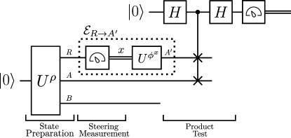
Figure 1: Test for separability of mixed states. The verifier uses a unitary circuit $U^{\rho}$ to produce the state $\psi_{RAB}$, which is a purification of $\rho_{AB}$. The prover (indicated by the dotted box) applies an entanglement-breaking channel $\mathcal{E}_{R\rightarrow A^{\prime}}$ on $R$ by measuring the rank-one POVM $\{\mu^{x}_{R}\}_{x}$ and then, depending on the outcome $x$, prepares a pure state from the set $\{\phi^{x}_{A^{\prime}}\}_{x}$. The final state is sent to the verifier, who performs a swap test. Theorem 1 states that the maximum acceptance probability of this interactive proof is equal to $\frac{1}{2}(1+F_{s}(\rho_{AB}))$, i.e., a simple function of the fidelity of separability.

Our separability test for mixed states consists of a distributed quantum computation involving a prover and a verifier. The computation (depicted in Figure 1) begins with the verifier preparing a purification $\psi_{RAB}$ of $\rho_{AB}$. The verifier sends the system $R$ to a quantum prover, whom, in our model, we restrict to performing entanglement-breaking channels. The prover thus performs an entanglement-breaking channel on the reference system $R$ and sends a system $A^{\prime}$ to the verifier. An entanglement-breaking channel $\mathcal{E}_{R\rightarrow A^{\prime}}$ can always be written as a measure-and-prepare channel [51], as follows:

$$\mathcal{E}_{R\rightarrow A^{\prime}}(\cdot)=\sum_{x\in\mathcal{X}}\operatorname{Tr}\left[\mu^{x}_{R}(\cdot)\right]\phi^{x}_{A^{\prime}},$$ (3)

where $\{\mu^{x}_{R}\}_{x\in\mathcal{X}}$ is a rank-one positive operator-valued measure (POVM) and $\{\phi^{x}_{A^{\prime}}\}_{x\in\mathcal{X}}$ is a set of pure states. (Due to the above measure-and-prepare decomposition of an entanglement-breaking channel, we can alternatively think of the prover as being split into two provers, a first who is allowed to perform a general quantum operation, followed by the communication of classical data to a second prover, who then is allowed to perform a general operation before communicating quantum data to the verifier. However, we proceed with the single-prover terminology in what follows.) By performing the measurement portion of the entanglement-breaking channel, the prover has in essence steered the verifier’s systems $A$ and $B$ to a certain probabilistic ensemble of pure states. After steering the verifier’s system, the prover then sends system $A^{\prime}$ to the verifier, by using the preparation portion of the entanglement-breaking channel. The verifier finally performs a swap test on system $A$ and $A^{\prime}$ and accepts if and only if the measurement outcome of the swap test is zero. The standard model in quantum computational complexity theory [41, 42] is that the prover is always trying to get the verifier to accept the computation: in this scenario, the prover steers the verifier’s systems $A$ and $B$ to an ensemble that has maximum overlap with a product-state ensemble and then sends an appropriate state to pass the swap test with the highest probability possible.

The maximum acceptance probability of the distributed quantum computation detailed above is equal to

$$\max_{\mathcal{E}\in\operatorname{EB}_{R\to A^{\prime}}}\operatorname{Tr}\left[\left(\Pi_{A^{\prime}A}^{\operatorname{sym}}\otimes I_{RB}\right)\mathcal{E}_{R\rightarrow A^{\prime}}\left(\psi_{RAB}\right)\right],$$ (4)

where $\Pi_{A^{\prime}A}^{\operatorname{sym}}$ is the projector onto the symmetric subspace of the $A^{\prime}$ and $A$ systems, and $\operatorname{EB}_{R\to A^{\prime}}$ denotes the set of all entanglement-breaking channels with input system $R$ and output system $A^{\prime}$. We find in Theorem 1 below that the maximum acceptance probability in (4) can be expressed as a simple function of the fidelity of separability of $\rho_{AB}$, the latter defined as [22, 23]

$$F_{s}(\rho_{AB})\coloneqq\max_{\sigma_{AB}\in\operatorname{SEP}(A:B)}F(\rho_{AB},\sigma_{AB}),$$ (5)

where $\operatorname{SEP}(A\!:\!B)$ denotes the set of separable states shared between Alice and Bob and $F(\rho,\sigma)\coloneqq\left\|\sqrt{\rho}\sqrt{\sigma}\right\|_{1}^{2}$ is the fidelity of the states $\rho$ and $\sigma$ [52]. The fidelity of separability is also known as the maximum separable fidelity [5, 6, 7]. With this definition, we state the first key theoretical result of our paper:

Theorem 1

For a pure state $\psi_{RAB}$, the following holds

$$\max_{\mathcal{E}\in\operatorname{EB}_{R\to A^{\prime}}}\operatorname{Tr}\left[\left(\Pi_{A^{\prime}A}^{\operatorname{sym}}\otimes I_{RB}\right)\mathcal{E}_{R\rightarrow A^{\prime}}\left(\psi_{RAB}\right)\right]\\ =\frac{1+F_{s}(\rho_{AB})}{2},$$ (6)

where $F_{s}(\rho_{AB})$ is the fidelity of separability of the state $\rho_{AB}=\operatorname{Tr}_{R}[\psi_{RAB}]$.

See the first part of Section 4 for a brief overview of the proof and Appendix A for a detailed proof. Appendices B and C recall some auxiliary results that support the proof in Appendix A. With this theorem, we have established a test of separability for mixed states.

There are two important aspects of our separability test we would like to point out in particular. First, note that the swap test at the end of the computation essentially leads to a measure of overlap between the state of the verifier’s system and the state provided to the verifier by the prover. The other important point is that, in the real world, there is no computationally unbounded quantum prover available to us to provide the ideal states required for the aforementioned tests.

Taking both these points into consideration, we modify the computation scenario in Figure 1 to a) measure the necessary overlaps directly and b) make use of quantum variational techniques [53] (parameterized unitary circuits and classical optimization of parameters) to approximate the actions of a computationally unbounded prover. The resulting procedure also tests and quantifies the separability of a given state by estimating its fidelity of separability. This procedure is a different sort of quantum variational technique, which we call a variational quantum steering algorithm (VQSA). As can be seen in Figure 2, quantum steering is at the core of the VQSA via the use of a parameterized mid-circuit measurement.

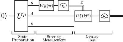
Figure 2: Quantum part of the VQSA to estimate the fidelity of separability $F_{s}(\rho_{AB})$. The unitary circuit $U^{\rho}$ prepares the state $\psi_{RAB}$, which is a purification of $\rho_{AB}$. The parameterized circuit $W_{R}(\Theta)$ acts on $R$ to evolve $\psi_{RAB}$ to another purification of $\rho_{AB}$. The measurement that follows, labeled “steering measurement,” steers the systems $AB$ to be in a pure state $\psi_{AB}^{x}$ if the measurement outcome $x$ occurs. Conditioned on the outcome $x$, the final parameterized circuit $U^{x}_{A}(\Theta^{x})$ and the subsequent measurement accepts with a maximum probability of $F_{s}(\rho_{AB})$.

Our VQSA is structured as follows. Let $\rho_{AB}$ denote the state for which we want to estimate the fidelity of separability, and let $\psi_{RAB}$ be a purification of it, which results from the action of the unitary operator $U^{\rho}$ on the all-zeros pure state $|0\rangle\!\langle 0|$. Once we have $\psi_{RAB}$, we can attempt to access all possible pure-state decompositions $\{(p(x),\psi_{AB}^{x})\}_{x\in\mathcal{X}}$ of $\rho_{AB}$ by acting on system $R$ with unitary operations. To do so, we use our first parameterized unitary $W_{R}(\Theta)$. To ensure that we have a sufficient number of measurement outcomes (to cover the possible case when $|\mathcal{X}|=\text{rank}(\rho_{AB})^{2}$), we can prepare some ancilla qubits in the all-zeros state, for a system $R^{\prime}$, and act with $W$ on $R$ and $R^{\prime}$. However, without loss of generality, these extra qubits can simply be lumped together as part of an overall reference system, relabeled as $R$.

After the action of $W_{R}(\Theta)$, the reference system is measured in the standard basis, and based on the outcome $x$, the post-measurement state of the system $AB$ is a pure state $\psi^{x}_{AB}$. We then estimate the maximum eigenvalue of the reduced state $\psi^{x}_{A}$: this can be accomplished by performing a parameterized unitary $U^{x}_{A}(\Theta^{x})$, based on the outcome $x$, on the reduced state $\psi_{A}^{x}$, measuring all qubits of $A$ in the computational basis, and accepting if the all-zeros outcome occurs.

Using a hybrid quantum–classical optimization loop, we can maximize the acceptance probability to estimate the value of the fidelity of separability. The quantum part of this VQSA is summarized in Figure 2.

Theorem 2

If the parameterized unitary circuits involved in the quantum part of the VQSA, summarized in Figure 2, can express all possible unitary operators of their respective systems, then the maximum acceptance probability of the quantum circuit is equal to $F_{s}(\rho_{AB})$.

See Appendix D for a detailed proof.

Since our algorithms will be running on near-term quantum computers that have limited scale and error tolerance, we develop semidefinite programs (SDPs) to benchmark the results from our VQSA because the ideal outcomes can be estimated classically for small numbers of qubits. Our benchmarks $\widetilde{F}_{s}^{1}(\rho_{AB},k)$ and $\widetilde{F}_{s}^{2}(\rho_{AB},k)$ are based on the positive partial transpose (PPT) and $k$-extendibility hierarchy. See details in Appendices E and F.

We now present an example simulation of our VQSA to demonstrate that it can obtain an estimate of the fidelity of separability. For the example, we take the state of interest $\rho_{AB}$ to be a ($3/4$,$1/4$) classical mixture of two maximally entangled states, $|\Phi^{+}\rangle=\sqrt{1/2}(|00\rangle+|11\rangle)$ and $|\Phi^{-}\rangle=\sqrt{1/2}(|00\rangle-|11\rangle)$, so that

$$\rho_{AB}=\frac{3}{4}|\Phi^{+}\rangle\!\langle\Phi^{+}|+\frac{1}{4}|\Phi^{-}\rangle\!\langle\Phi^{-}|.$$ (7)

Systems $R$, $A$, and $B$ of the purification of $\rho_{AB}$ contain one qubit each. See Figure 3 for the results. We use the benchmarks and VQSA to estimate the fidelity of separability and that they converge to 0.93. We evaluate these benchmarks for different levels of the $k$-extendibility hierarchy. See Appendix G for more examples and Appendix H for details about the code we developed.

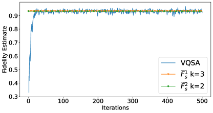
Figure 3: Fidelity of separability calculated for a ($3/4$,$1/4$) classical mixture of $|\Phi^{+}\rangle$ and $|\Phi^{-}\rangle$ using our VQSA (blue line). The algorithm converges to 0.93, which agrees with the value obtained using the benchmarks $\widetilde{F}_{s}^{1}$ and $\widetilde{F}_{s}^{2}$.

We also generalize our VQSA to measure the fidelity of separability of multipartite states in the following fashion. A multipartite state $\rho_{A_{1}\cdots A_{M}}\in\mathcal{D}(\mathcal{H}_{A_{1}\cdots A_{M}})=\mathcal{D}(\mathcal{H}_{A_{1}}\otimes\cdots\otimes\mathcal{H}_{A_{M}})$ is separable if it can be written as

$$\rho_{A_{1}\cdots A_{M}}=\sum_{x\in\mathcal{X}}p(x)\psi^{x,1}_{A_{1}}\otimes\cdots\otimes\psi^{x,M}_{A_{M}}$$ (8)

where $\psi_{A_{i}}^{x,i}$ is a pure state for every $x\in\mathcal{X}$ and $i\in\{1,\ldots,M\}$. Let $M\text{-SEP}$ denote the set of all $\rho_{A_{1}\cdots A_{M}}\in\mathcal{D}(\mathcal{H}_{A_{1}\cdots A_{M}})$ such that $\rho_{A_{1}\cdots A_{M}}$ is separable.

For the multipartite case of the distributed quantum computation, the verifier prepares a purification $\psi^{\rho}_{R^{\prime}A_{1}\cdots A_{M}}$ of $\rho_{A_{1}\cdots A_{M}}$. The prover applies a multipartite entanglement-breaking channel on $R$, which can be written as:

$$\mathcal{E}_{R\rightarrow A^{\prime}_{1}\cdots A^{\prime}_{M-1}}(\cdot)\\ =\sum_{x\in\mathcal{X}}\operatorname{Tr}[\mu^{x}_{R}(\cdot)]\left(\phi^{x,1}_{A^{\prime}_{1}}\otimes\cdots\otimes\phi^{x,M-1}_{A^{\prime}_{M-1}}\right),$$ (9)

where $\{\mu^{x}_{R}\}_{x}$ is a rank-one POVM and $\{\phi^{x,i}_{A^{\prime}_{i}}\}_{x,i}$ is a set of pure states. The prover sends systems $(A^{M-1})^{\prime}\equiv A^{\prime}_{1}\cdots A^{\prime}_{M-1}$ to the verifier. Finally, the verifier performs a collective swap test on these systems and the systems $A_{1}\cdots A_{M}$, as depicted in Figure 4. The acceptance probability of this distributed quantum computation is given by

$$\max_{\mathcal{E}\in\operatorname{EB}_{M-1}}\operatorname{Tr}[\Pi_{(A^{M-1})^{\prime}A^{M-1}}^{\operatorname{sym}}\mathcal{E}_{R\rightarrow(A^{M-1})^{\prime}}(\psi_{RA^{M-1}})],$$ (10)

where $\Pi_{(A^{M-1})^{\prime}A^{M-1}}^{\operatorname{sym}}$ is the projection onto the symmetric subspace of systems $(A^{M-1})^{\prime}$ and $A^{M-1}$ and $\operatorname{EB}_{M-1}$ denotes the set of multipartite entanglement-breaking channels defined in (9). This leads to the following theorem:

Theorem 3

For a pure state $\psi_{RA^{M}}\equiv\psi_{RA_{1}\cdots A_{M}}$, the following equality holds:

$$\max_{\mathcal{E}\in\operatorname{EB}_{M-1}}\operatorname{Tr}[\Pi_{(A^{M-1})^{\prime}(A^{M-1})}^{\operatorname{sym}}\mathcal{E}_{R\rightarrow A^{\prime}_{1}\cdots A^{\prime}_{M-1}}(\psi_{RA^{M}})]\\ =\frac{1}{2}\left(1+F_{s}(\rho_{A_{1}\cdots A_{M}})\right),$$ (11)

where the multipartite fidelity of separability is defined as

$$F_{s}(\rho_{A_{1}\cdots A_{M}})\coloneqq\\ \max_{\sigma_{A_{1}\cdots A_{M}}\in M-\operatorname{SEP}}F(\rho_{A_{1}\cdots A_{M}},\sigma_{A_{1}\cdots A_{M}}).$$ (12)

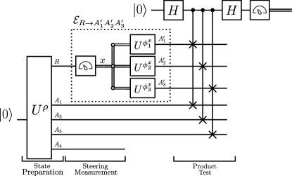
Figure 4: Test for separability of multipartite mixed states. The verifier uses the unitary circuit $U^{\rho}$ to prepare the state $\psi_{RA_{1}A_{2}A_{3}A_{4}}$, which is a purification of $\rho_{A_{1}A_{2}A_{3}A_{4}}$. The prover (indicated by the dotted box) applies an entanglement-breaking channel $\mathcal{E}_{R\rightarrow A^{\prime}_{1}A^{\prime}_{2}A^{\prime}_{3}}$ on $R$ by measuring the rank-one POVM $\{\mu^{x}_{R}\}_{x\in\mathcal{X}}$ and then, depending on the outcome $x$, prepares a state from the set $\{\phi^{x,1}_{A^{\prime}_{1}}\otimes\phi^{x,2}_{A^{\prime}_{2}}\otimes\phi^{x,3}_{A^{\prime}_{3}}\}_{x\in\mathcal{X}}$. The final state is sent to the verifier, who performs a collective swap test. Theorem 10 states that the maximum acceptance probability of this interactive proof is equal to $\frac{1}{2}(1+F_{s}(\rho_{A_{1}A_{2}A_{3}A_{4}}))$, i.e., a simple function of the fidelity of separability.

See Appendix I for a proof. We can then use the generalized test of separability of mixed states to develop a VQSA for the multipartite case. See Figure 5. This involves replacing the collective swap test in Figure 4 with an overlap measurement, similar to how we got Figure 2 from Figure 1.

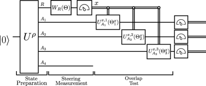
Figure 5: VQSA to estimate the multipartite fidelity of separability $F_{s}(\rho_{A_{1}A_{2}A_{3}A_{4}})$. The unitary circuit $U^{\rho}$ prepares the state $\psi_{RA_{1}A_{2}A_{3}A_{4}}$, which is a purification of $\rho_{A_{1}A_{2}A_{3}A_{4}}$. The parameterized circuit $W_{R}(\Theta)$ acts on $R$ to evolve the state to another purification of $\rho_{A_{1}A_{2}A_{3}A_{4}}$. The measurement that follows, labeled “steering measurement,” steers the remaining systems to be in a state $\psi_{A_{1}A_{2}A_{3}A_{4}}^{x}$, if the measurement outcome $x$ occurs. Conditioned on the outcome $x$, the final parameterized circuits $U^{x,1}_{A_{1}}(\Theta^{x}_{1})$, $U^{x,2}_{A_{2}}(\Theta^{x}_{2})$, and $U^{x,3}_{A_{3}}(\Theta^{x}_{3})$ are applied and the subsequent measurement accepts with a maximum probability of $F_{s}(\rho_{A_{1}A_{2}A_{3}A_{4}})$.

Our final result is regarding the computational complexity of estimating the fidelity of separability $F_{s}(\rho_{AB})$. The complexity-theoretic approach gives us a way to classify the separability problem based on its difficulty and complexity. Analyses of this form can be effectively conducted within the framework of quantum computational complexity theory [41, 42].

In the paradigm of complexity theory [54], a complexity class is a set of computational problems that require similar resources to solve. If a complexity class $A$ is contained within another class $B$, then some problems in $B$ could require more computational resources to solve than problems in $A$. To effectively characterize the difficulty of a class of problems, we pick a problem that is representative of the class, or complete for the class. A problem $h$ is said to be complete for a complexity class $A$ if $h$ is contained in the class and the ability to solve problem $h$ can be extended efficiently to solve every other problem in $A$.

To tackle the question posed about the computational complexity of estimating the fidelity of separability, we define QIP${}_{\operatorname{EB}}(2)$ to be the complexity class containing problems that can be solved using a prover restricted to using only entanglement-breaking channels, which processes a quantum message received from the verifier and sends back a quantum message to the verifier. Thus, estimating the fidelity of separability of a given state then falls within QIP${}_{\operatorname{EB}}(2)$, as can be seen from Figure 1. To fully characterize this novel complexity class, we provide a complete problem for it. We establish that, given quantum circuits to generate a channel $\mathcal{N}_{A\rightarrow B}$ and a state $\rho_{B}$, estimating the following quantity is complete for QIP${}_{\operatorname{EB}}(2)$:

$$\max_{\begin{subarray}{c}\{(p(x),\psi^{x})\}_{x},\left\{\varphi^{x}\right\}_{x},\\ \rho_{B}=\sum_{x}p(x)\psi_{B}^{x}\end{subarray}}\sum_{x}p(x)F(\psi_{B}^{x},\mathcal{N}_{A\rightarrow B}(\varphi_{A}^{x})).$$ (13)

See Appendix J for details, as well as an interpretation of this problem.

By placing the problem of estimating the fidelity of separability in the class QIP${}_{\operatorname{EB}}(2)$, we establish results that link quantum steering and the separability problem to quantum computational complexity theory. Furthermore, we show that the complexity class QIP${}_{\operatorname{EB}}(2)$ is contained in QIP [55, 56], and contains QAM [57] and QSZK [58]. It also follows, as a direct generalization of the hardness results from [5, 6], that the problem of estimating the fidelity of separability is hard for QSZK and NP. All of the aforementioned complexity classes are considered to be, in the worst case, out of reach of the capabilities of efficient quantum computers. See Appendix K for proofs and Figure 6 for a detailed diagram. However, following the approach of [59], we can try to solve some instances of problems in these classes using parameterized circuits and VQAs.

Figure 6: Placement of QIP${}_{\operatorname{EB}}(2)$ relative to other known complexity classes. The complexity classes are organized such that if a class is connected to a class above it, the complexity class placed lower is a subset of the class above. For example, QIP${}_{\operatorname{EB}}(2)$ is subset of QIP and QIP${}_{\operatorname{EB}}(2)$ is a superset of both QMA and QAM.

3 Conclusion and Discussion

In this paper, we detailed a distributed quantum computation to test the separability of a quantum state that, at its core, makes use of quantum steering. Through this test, we demonstrated a link between quantum steering and the separability problem. The acceptance probability of this distributed quantum computation is directly related to an entanglement measure known as the fidelity of separability. We also showed computational complexity-theoretic results and established a link between quantum steering, quantum algorithms, and quantum computational complexity using the structure of the test. By replacing the prover with a parameterized circuit, we modified this distributed quantum computation to develop our VQSA, which is a novel kind of variational quantum algorithm that uses quantum steering to address the problem of estimating the fidelity of separability. This algorithm allows for the direct estimation of the fidelity of separability, without the need for state tomography and subsequent approximate tests on separability. Here we note that our algorithm is not unitary, due to the mid-circuit measurement on system $R$ and the consequent conditional operation that is applied on system $A$. This is an important distinction from most VQAs, which do not make use of a parameterized mid-circuit measurement. We also discuss multipartite generalizations of both our separability test and VQSA. Finally, we simulated our VQSA using the noisy Qiskit Aer simulator and showed favorable convergence trends, which were compared against two classical SDP benchmarks.

Our VQSA has applications beyond entanglement quantification on a single quantum computer. We can also think of our VQSA as a distributed variational quantum algorithm for measuring the entanglement of a bipartite state. See [60, 61, 62] for previous instances of distributed VQAs. Indeed, our algorithm can be executed over a quantum network in which each node in the network has quantum and classical computers capable of performing VQAs. The initial part of the algorithm distributes $R$ to Rob, $A$ to Alice, and $B$ to Bob, who are all in distant locations. Then Rob performs the parameterized measurement, sends the outcome over a classical channel to Alice, who then performs another parameterized measurement. Then they can repeat this process to assess the quality of the entanglement between Alice and Bob. This interpretation is even more interesting in terms of quantum networks for the multipartite case, in which the classical data gets broadcast from Rob to all the other nodes, with the exception of the last one.

VQSAs can be used to tackle other problems that involve quantum steering, like maximization of pure-state decompositions of quantum states. This technique may also be useful for estimating other entanglement measures that involve an optimization over the set of separable states. By applying the insights of [63, Appendix A] and our approach here, it is clear that VQSAs will also be useful for estimating maximal fidelities associated with other resource theories, such as the resource theory of coherence [64]. More broadly, we suspect that the paradigm of parameterized mid-circuit measurements and distributed variational quantum algorithms will be useful in addressing other computational problems of interest in quantum information science and physics, given recent advances in experimental implementations [65, 66, 67, 68].

4 Methods

In this section, we provide a short overview of the techniques used to prove Theorem 1, our main result, along with a brief description of SDP benchmarks and important details about our simulations.

To gain intuition about the separability test for mixed states, let us formulate a simple test for the separability of pure states. From (1), we can see that a pure bipartite state $\varphi_{AB}$ is separable if it can be written in product form, as

$$\varphi_{AB}=\psi_{A}\otimes\phi_{B},$$ (14)

where $\psi_{A}$ and $\phi_{B}$ are pure states. The test that we develop below is important because it will reappear as part of the test for separability in the general case, along with quantum steering. Additionally, our approach is slightly different from the standard approach for testing entanglement of pure states, which employs two copies of the state in a swap test [69, 70, 7]. Instead, our approach requires only a single copy of the state.

Our pure-state separability test consists of a distributed quantum computation involving a prover and a verifier (see Figure 7). The computation starts with the verifier preparing the pure state $\psi_{AB}$. The prover sends the verifier the pure state $\phi_{A^{\prime}}$ in register $A^{\prime}$. (We note that the prover can send a mixed state; however, the maximum acceptance probability of the test is achieved by a pure state. Hence, without loss of generality, it suffices for the prover to send a pure state.) The verifier then performs the standard swap test [71, 72] on $A$ and $A^{\prime}$ and accepts if the measurement outcome is zero. In the standard model of quantum computational complexity [41, 42], the prover attempts to get the verifier to accept the swap test with as high a probability as possible. Thus, in this scenario, the prover selects $\phi_{A^{\prime}}$ to maximize the overlap between the reduced stated $\psi_{A}\coloneqq\operatorname{Tr}_{B}[\psi_{AB}]$ and $\phi_{A^{\prime}}$. The maximum acceptance probability is then equal to

$$\max_{\phi}\operatorname{Tr}[(\Pi_{A^{\prime}A}^{\operatorname{sym}}\otimes I_{B})(\phi_{A^{\prime}}\otimes\psi_{AB})]$$

$$=\frac{1}{2}\left(1+\max_{\phi}\operatorname{Tr}[F_{A^{\prime}A}(\phi_{A^{\prime}}\otimes\psi_{A})]\right)$$ (15)

$$=\frac{1}{2}\left(1+\max_{\phi}\operatorname{Tr}[\phi_{A}\psi_{A}]\right)=\frac{1}{2}\left(1+\left\|\psi_{A}\right\|_{\infty}\right),$$ (16)

where $F_{A^{\prime}A}$ is the unitary swap operator acting on systems $A^{\prime}$ and $A$, the projector $\Pi_{A^{\prime}A}^{\operatorname{sym}}\coloneqq\frac{1}{2}\left(I_{A^{\prime}A}+F_{A^{\prime}A}\right)$ projects onto the symmetric subspace of $A^{\prime}$ and $A$, and $\left\|\psi_{A}\right\|_{\infty}$ is the spectral norm of the reduced state $\psi_{A}$ (equal to its largest eigenvalue). Since $\left\|\psi_{A}\right\|_{\infty}=1$ if and only if $\psi_{A}$ is a pure state and this occurs if and only if $\psi_{AB}$ is a product state, it follows that the maximal acceptance probability is equal to one if and only if $\psi_{AB}$ is a product state.

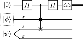
Figure 7: Pure-state separability test: The verifier is in possession of the pure state $\psi_{AB}$ of interest. The prover (indicated by the dotted box) sends the verifier a pure state $\phi_{A^{\prime}}$, who then performs the standard swap test on systems $A^{\prime}$ and $A$. As mentioned in (16), the acceptance probability is equal to $\frac{1}{2}(1+\left\|\psi_{A}\right\|_{\infty})$.

Now we outline the proof of Theorem 1, which relies on two important facts. The first is that the fidelity of separability can be written in terms of a convex roof as follows [63, Theorem 1]:

$$F_{s}(\rho_{AB})=\max_{\begin{subarray}{c}\{(p(x),\psi_{AB}^{x})\}_{x},\\ \rho_{AB}=\sum_{x}p(x)\psi_{AB}^{x}\end{subarray}}\sum_{x}p(x)F_{s}(\psi_{AB}^{x}),$$ (17)

where $\{p(x)\}_{x}$ is a probability distribution and each $\psi_{AB}^{x}$ is a pure state. See also [73, Lemma 1]. The second fact is that, for a pure bipartite state, $F_{s}(\psi_{AB})$ can be rewritten as [63, Section 6.2]

$$F_{s}(\psi_{AB})=\left\|\psi_{A}\right\|_{\infty}.$$ (18)

Along with these facts, we also note that the optimization over all entanglement-breaking channels in (4) is the same as optimizing over all pure-state decompositions of $\rho_{AB}$ and the rest of the proof follows. For completeness, we provide proofs of (17) and (18) in Appendices B and C, respectively. It follows from (1) and (18) that $\sum_{x}p(x)\left\|\psi_{A}^{x}\right\|_{\infty}=1$ for a separable state, which is the maximum possible value of $F_{s}(\rho_{AB})$. Hence the distributed quantum computation in Figure 1 tests and quantifies the separability of a state, by estimating its fidelity of separability. However, we note that there are complexity-theoretic subtleties associated with the parallel repetition of this algorithm, which we discuss in detail in Appendix K.4. Finally, note that the computation in Figure 1 can be reduced to that in Figure 7 if the purifying system $R$ is trivial, implying that the verifier only prepares a pure state on systems $A$ and $B$ in this case.

Benchmarking via semidefinite programs.— Here we briefly explain the derivation of the SDP benchmarks $\widetilde{F}_{s}^{1}(\rho_{AB},k)$ and $\widetilde{F}_{s}^{2}(\rho_{AB},k)$.

First, let us recall that the fidelity between two quantum states has an SDP formulation [74]. Since there is no semidefinite constraint that directly corresponds to optimizing over the set of separable states [75], we can approximate the fidelity of separability of a state by maximizing its fidelity with positive partial transpose (PPT) states [27, 28] and $k$-extendible states [29, 30]. Further noting that the PPT and $k$-extendibility constraints are positive semidefinite constraints, we obtain our first benchmark $\widetilde{F}_{s}^{1}(\rho_{AB},k)$, defined in Appendix E, and which is proven there to satisfy the following bounds:

$$F_{s}(\rho_{AB})\leq\widetilde{F}_{s}^{1}(\rho_{AB},k)\\ \leq 1-\left[\sqrt{1-F_{s}(\rho_{AB})}-2\sqrt{\frac{\left|B\right|^{2}}{k}\left(1-\frac{\left|B\right|^{2}}{k}\right)}\right]^{2},$$ (19)

where $\left|B\right|$ is the dimension of system $B$. By inspection of the above inequalities, observe that

$$\lim_{k\to\infty}\widetilde{F}_{s}^{1}(\rho_{AB},k)=F_{s}(\rho_{AB}).$$ (20)

The second benchmark can be obtained using (4). Just like PPT and $k$-extendible states were used to approximate separable states for the first benchmark, we use PPT channels [76, 77] and $k$-extendible channels [78, 79, 80, 81] to approximate entanglement-breaking channels, leading to our second benchmark $\widetilde{F}_{s}^{2}(\rho_{AB},k)$. We show that $\widetilde{F}_{s}^{2}(\rho_{AB},k)$ is an SDP and approximates the fidelity of separability in the following fashion:

$$F_{s}(\rho_{AB})\leq\widetilde{F}_{s}^{2}(\rho_{AB},k)\leq F_{s}(\rho_{AB})+\frac{4\left|A\right|^{3}\left|B\right|}{k}.$$ (21)

where $\left|A\right|$ and $\left|B\right|$ is the dimension of systems $A$ and $B$, respectively. See Appendix F for a proof. Again, observe that

$$\lim_{k\to\infty}\widetilde{F}_{s}^{2}(\rho_{AB},k)=F_{s}(\rho_{AB}).$$ (22)

Simulations and Reward Functions.—For our simulations, we use the Qiskit Aer simulator and Qiskit’s Simultaneous Perturbation Stochastic Approximation (SPSA) optimizer to perform the classical optimization. The jitters in the fidelity values between iterations of the VQSA can be attributed to the shot noise in estimating the acceptance probability, using the Qiskit Aer simulator, as well as the fact that the SPSA optimizer we have used to perform the classical optimization is itself a stochastic algorithm. We provide more examples in Appendix G.

An important issue with variational quantum techniques, such as VQAs, is the emergence of barren plateaus or vanishing gradients as the number of qubits involved increases [43]. However, recent results have shown that this problem can be mitigated by switching from a global reward function to a local reward function [44]. In our case, a global reward function is one in which we measure all the qubits that constitute system $A$, as done in the approach discussed in Theorem 2. An example of a local reward function is one involving selecting a qubit in system $A$ at random to measure in the computational basis and recording the outcome, accepting if the outcome is equal to zero. Our proposed local reward function can be used to obtain upper and lower bounds on our initial global reward function, following the approach of [82, Appendix C] and discussed for completeness in Appendix L. Local functions have also been used to avoid barren plateaus in VQAs to determine the geometric measure of entanglement for pure states [83]. We provide simulations of the local reward function in Appendix G, indicating that the local reward function can also be used to obtain an estimate on the fidelity of separability of a given state.

Appendix A Proof of Theorem 1

In this appendix, we prove Theorem 1, showing that the acceptance probability of the first test of separability for mixed states is equal to $\frac{1}{2}\left(1+F_{s}(\rho_{AB})\right)$.

Proof of Theorem 1. Recall that an entanglement-breaking channel can be rewritten as

$$\mathcal{E}_{R\rightarrow A^{\prime}}(\cdot)=\sum_{x}\operatorname{Tr}[\mu^{x}_{R}(\cdot)]\phi^{x}_{A^{\prime}},$$ (23)

where $\{\mu^{x}_{R}\}_{x}$ is a rank-one POVM and $\{\phi^{x}_{A^{\prime}}\}_{x}$ is a set of pure states. Then we find, for fixed $\mathcal{E}_{R\rightarrow A^{\prime}}$, that

$$\operatorname{Tr}[\Pi_{A^{\prime}A}^{\operatorname{sym}}\mathcal{E}_{R\rightarrow A^{\prime}}(\psi_{RAB})] =\frac{1}{2}\operatorname{Tr}[(I_{A^{\prime}A}+F_{A^{\prime}A})\mathcal{E}_{R\rightarrow A^{\prime}}(\psi_{RAB})]$$ (24)

$$=\frac{1}{2}\left(1+\operatorname{Tr}[F_{A^{\prime}A}\mathcal{E}_{R\rightarrow A^{\prime}}(\psi_{RAB})]\right).$$ (25)

So let us work with the expression $\operatorname{Tr}[F_{A^{\prime}A}\mathcal{E}_{R\rightarrow A^{\prime}}(\psi_{RAB})]$. Consider that

$$\operatorname{Tr}[F_{A^{\prime}A}\mathcal{E}_{R\rightarrow A^{\prime}}(\psi_{RAB})] =\operatorname{Tr}\!\left[F_{A^{\prime}A}\sum_{x}\operatorname{Tr}_{R}[\mu^{x}_{R}\psi_{RAB}]\otimes\phi^{x}_{A^{\prime}}\right]$$ (26)

$$=\operatorname{Tr}\!\left[F_{A^{\prime}A}\sum_{x}p(x)\psi_{AB}^{x}\otimes\phi^{x}_{A^{\prime}}\right]$$ (27)

$$=\operatorname{Tr}\!\left[F_{A^{\prime}A}\sum_{x}p(x)\psi_{A}^{x}\otimes\phi^{x}_{A^{\prime}}\right]$$ (28)

$$=\sum_{x}p(x)\langle\phi^{x}|_{A}\psi_{A}^{x}|\phi^{x}\rangle_{A},$$ (29)

where

$$p(x) \coloneqq\operatorname{Tr}[\mu^{x}_{R}\psi_{RAB}],$$ (30)

$$\psi_{AB}^{x} \coloneqq\frac{1}{p(x)}\operatorname{Tr}_{R}[\mu^{x}_{R}\psi_{RAB}].$$ (31)

Thus, the acceptance probability for a fixed entanglement-breaking channel is given by

$$\operatorname{Tr}[\Pi_{A^{\prime}A}^{\operatorname{sym}}\mathcal{E}_{R\rightarrow A^{\prime}}(\psi_{RAB})]=\frac{1}{2}\left(1+\sum_{x}p(x)\langle\phi^{x}|_{A}\psi_{A}^{x}|\phi^{x}\rangle_{A}\right).$$ (32)

After optimizing over every element of $\operatorname{EB}_{R\to A^{\prime}}$, which denotes the set of all entanglement-breaking channels with input system $R$ and output system $A^{\prime}$, and realizing that optimizing over measurements in $\mathcal{E}_{R\rightarrow A^{\prime}}$ induces a pure-state decomposition of $\rho_{AB}$ and optimizing over preparation channels in $\mathcal{E}_{R\rightarrow A^{\prime}}$ gives the spectral norm of $\psi_{A}^{x}$, we find the claimed formula for the acceptance probability, when combined with the development in Appendices B and C:

$$\max_{\mathcal{E}\in\operatorname{EB}_{R\to A^{\prime}}}\operatorname{Tr}[(\Pi_{A^{\prime}A}^{\operatorname{sym}}\otimes I_{RB})\mathcal{E}_{R\rightarrow A^{\prime}}(\psi_{RAB})]=\frac{1+F_{s}(\rho_{AB})}{2}.$$ (33)

This concludes the proof.   

Appendix B Alternative Proof of Equation (17)

In this appendix, we provide an alternative proof for Theorem 1 in [63]. This proof relies on Uhlmann’s theorem [52], the triangle inequality, and the Cauchy–Schwarz inequality. See also [73, Lemma 1].

Theorem 4 ([63])

The following formula holds

$$F_{s}(\rho_{AB})=\max_{\left\{(p(x),\psi_{AB}^{x})\right\}_{x}}\left\{\sum_{x}p(x)F_{s}(\psi_{AB}^{x}):\rho_{AB}=\sum_{x}p(x)\psi_{AB}^{x}\right\},$$ (34)

where $\{(p(x),\psi_{AB}^{x})\}_{x}$ satisfies $\sum_{x}p(x)\psi_{AB}^{x}=\rho_{AB}$, all $\psi_{AB}^{x}$ are pure, and

$$F_{s}(\psi_{AB})=\max_{|\phi\rangle_{A},|\varphi\rangle_{B}}|\langle\psi|_{AB}|\phi\rangle_{A}\otimes|\varphi\rangle_{B}|^{2}.$$ (35)

Proof. Since the definition in (5) requires an optimization over all separable states, we take $\left|\mathcal{X}\right|=\left(\left|A\right|\left|B\right|\right)^{2}$. The separable state in (1) is purified by

$$|\psi^{\sigma}\rangle_{RAB}=\sum_{x\in\mathcal{X}}\sqrt{p(x)}|x\rangle_{R}|\psi^{x}\rangle_{A}|\phi^{x}\rangle_{B}.$$ (36)

Now consider a generic purification $|\psi^{\rho}\rangle_{R^{\prime}AB}$ of $\rho_{AB}$. Recall that the dimension of the purifying system $R^{\prime}$ satisfies rank$(\rho_{AB})\leq\left|R^{\prime}\right|$ and so we can simply set $\left|R^{\prime}\right|=\left|A\right|\left|B\right|$. Taking $R^{\prime\prime}$ to be a system of dimension $\left|A\right|\left|B\right|$, we then have that

$$|\psi^{\rho}\rangle_{R^{\prime}AB}|0\rangle_{R^{\prime\prime}}$$ (37)

purifies $\rho_{AB}$. Applying Uhlmann’s theorem [52], the maximum separable root fidelity can be written as

$$\max_{\sigma_{AB}\in\operatorname{SEP}(A:B)}\sqrt{F}(\rho_{AB},\sigma_{AB})=\\ \max_{\begin{subarray}{c}U,\\ \left\{\left(p(x),\psi^{x}{}_{A},\phi_{B}^{x}\right)\right\}_{x}\end{subarray}}\left|\left(\sum_{x^{\prime}}\sqrt{p(x^{\prime})}\langle x^{\prime}|_{R}\langle\psi^{x^{\prime}}|_{A}\langle\phi^{x^{\prime}}|_{B}\right)\left(U_{R^{\prime}R^{\prime\prime}\rightarrow R}\otimes I_{AB}\right)|\psi^{\rho}\rangle_{R^{\prime}AB}|0\rangle_{R^{\prime\prime}}\right|,$$ (38)

where the maximization is over every unitary $U_{R^{\prime}R^{\prime\prime}\rightarrow R}$. Expanding $U_{R^{\prime}R^{\prime\prime}\rightarrow R}|\psi^{\rho}\rangle_{R^{\prime}AB}|0\rangle_{R^{\prime\prime}}$ in terms of the standard basis $|x\rangle$ as

$$U_{R^{\prime}R^{\prime\prime}\rightarrow R}|\psi^{\rho}\rangle_{R^{\prime}AB}|0\rangle_{R^{\prime\prime}}=\sum_{x\in\mathcal{X}}\sqrt{q(x)}|x\rangle_{R}|\varphi^{x}\rangle_{AB},$$ (39)

we note that $U$ followed by a measurement in the standard basis induces a convex decomposition of $\rho_{AB}$ in terms of the ensemble $\{(q(x),\varphi_{AB}^{x})\}_{x}$. We can write the root fidelity as

$$\max_{\sigma_{AB}\in\operatorname{SEP}(A:B)}\sqrt{F}(\rho_{AB},\sigma_{AB}) =\max_{\begin{subarray}{c}\left\{\left(p(x),\psi^{x}{}_{A},\phi_{B}^{x}\right)\right\}_{x},\\ \{(q(x),\varphi_{AB}^{x})\}_{x}\end{subarray}}\left|\sum_{x,x^{\prime}}\-\sqrt{q(x)p(x^{\prime})}\langle x|x^{\prime}\rangle_{R}\langle\varphi^{x}|_{AB}|\psi^{x^{\prime}}\rangle_{A}|\phi^{x^{\prime}}\rangle_{B}\right|$$

$$=\max_{\begin{subarray}{c}\left\{\left(p(x),\psi^{x}{}_{A},\phi_{B}^{x}\right)\right\}_{x},\\ \{(q(x),\varphi_{AB}^{x})\}_{x}\end{subarray}}\left|\sum_{x}\sqrt{q(x)p(x)}\langle\varphi^{x}|_{AB}|\psi^{x}\rangle_{A}|\phi^{x}\rangle_{B}\right|$$ (40)

$$=\max_{\begin{subarray}{c}\left\{\left(p(x),\psi^{x}{}_{A},\phi_{B}^{x}\right)\right\}_{x},\\ \{(q(x),\varphi_{AB}^{x})\}_{x}\end{subarray}}\left|\sum_{x}\sqrt{q(x)p(x)}\langle\varphi^{x}|_{AB}|\psi^{x}\rangle_{A}|\phi^{x}\rangle_{B}\right|.$$ (41)

Next, for fixed $\left\{\left(p(x),\psi^{x}{}_{A},\phi_{B}^{x}\right)\right\}_{x}$ and $\{(q(x),\varphi_{AB}^{x})\}_{x}$, we bound the objective function in the optimization above as follows:

$$\left|\sum_{x}\sqrt{q(x)p(x)}\langle\varphi^{x}|_{AB}|\psi^{x}\rangle_{A}|\phi^{x}\rangle_{B}\right| \leq\sum_{x}\sqrt{p(x)q(x)}\left|\langle\varphi^{x}|_{AB}|\psi^{x}\rangle_{A}|\phi^{x}\rangle_{B}\right|$$ (42)

$$\leq\sqrt{\sum_{x}p(x)}\sqrt{\sum_{x}q(x)\left|\langle\varphi^{x}|_{AB}|\psi^{x}\rangle_{A}|\phi^{x}\rangle_{B}\right|^{2}}$$ (43)

$$=\sqrt{\sum_{x}q(x)\left|\langle\varphi^{x}|_{AB}|\psi^{x}\rangle_{A}|\phi^{x}\rangle_{B}\right|^{2}}.$$ (44)

The first inequality follows from the triangle inequality and the second from an application of Cauchy–Schwarz. We see that equality is achieved in the second inequality by choosing

$$p(x)=\frac{q(x)\left|\langle\varphi^{x}|_{AB}|\psi^{x}\rangle_{A}|\phi^{x}\rangle_{B}\right|^{2}}{\sum_{x}q(x)\left|\langle\varphi^{x}|_{AB}|\psi^{x}\rangle_{A}|\phi^{x}\rangle_{B}\right|^{2}}.$$ (45)

We can achieve equality in the first inequality by tuning a global phase for the state $|\psi^{x}\rangle_{A}$, which amounts to a relative phase in (36). Putting everything together, we conclude that

$$\max_{\sigma_{AB}\in\operatorname{SEP}}F(\rho_{AB},\sigma_{AB})=\max_{\{(q(x),\varphi_{AB}^{x})\}_{x}}\sum_{x}q(x)\max_{\left(|\psi^{x}\rangle_{A}|\phi^{x}\rangle_{B}\right)_{x},}\left|\langle\varphi^{x}|_{AB}|\psi^{x}\rangle_{A}|\phi^{x}\rangle_{B}\right|^{2},$$ (46)

which is equivalent to the desired equality in (17).   

Appendix C Proof of Equation (18)

In this appendix, we show that the fidelity of separability of a bipartite state can be written in terms of the spectral norm, which was also observed in [63, Section 6.2].

Proposition 5

For a bipartite state, the following equality holds

$$F_{s}(\rho_{AB})=\max_{\left\{(p(x),\psi_{AB}^{x})\right\}_{x}}\left\{\sum_{x}p(x)\left\|\psi_{A}^{x}\right\|_{\infty}:\rho_{AB}=\sum_{x}p(x)\psi_{AB}^{x}\right\}.$$ (47)

Proof. Consider that the following holds for a pure bipartite state $\psi_{AB}$:

$$F_{s}(\psi_{AB}) =\max_{|\phi\rangle_{A},|\varphi\rangle_{B}}\left|\langle\psi|_{AB}|\phi\rangle_{A}\otimes|\varphi\rangle_{B}\right|^{2}$$ (48)

$$=\max_{|\phi\rangle_{A},|\varphi\rangle_{B}}\left|\langle\phi|_{A}\otimes\langle\varphi|_{B}|\psi\rangle_{AB}\right|^{2}$$ (49)

$$=\max_{|\phi\rangle_{A}}\left\|\langle\phi|_{A}\otimes I_{B}|\psi\rangle_{AB}\right\|_{2}^{2}$$ (50)

$$=\max_{|\phi\rangle_{A}}\operatorname{Tr}[(|\phi\rangle\!\langle\phi|_{A}\otimes I_{B})\psi_{AB}]$$ (51)

$$=\max_{|\phi\rangle_{A}}\operatorname{Tr}[|\phi\rangle\!\langle\phi|_{A}\psi_{A}]$$ (52)

$$=\left\|\psi_{A}\right\|_{\infty}.$$ (53)

The first two equalities follow from the definition and a rewriting. The third equality follows from the variational characterization of the Euclidean norm of a vector. The fourth equality follows because

$$\left\|\langle\phi|_{A}\otimes I_{B}|\psi\rangle_{AB}\right\|_{2}^{2} =\left(\langle\psi|_{AB}|\phi\rangle_{A}\otimes I_{B}\right)\left(\langle\phi|_{A}\otimes I_{B}|\psi\rangle_{AB}\right)$$ (54)

$$=\langle\psi|_{AB}|\phi\rangle\!\langle\phi|_{A}\otimes I_{B}|\psi\rangle_{AB}$$ (55)

$$=\operatorname{Tr}[(|\phi\rangle\!\langle\phi|_{A}\otimes I_{B})\psi_{AB}].$$ (56)

The next follows from taking a partial trace, and the final equality from the variational characterization of the spectral norm. So this implies the desired equality, after applying (17).   

Appendix D Proof of Theorem 2

In this appendix, we show that the acceptance probability of our VQSA is indeed equal to $F_{s}(\rho_{AB})$ if the parameterized unitary circuits can express all possible unitary operators of their respective systems. For this, let us track the state of the VQSA at the points indicated in Figure 8.

• At Step $(1)$, the unitary $U^{\rho}$ prepares the pure state $\psi_{RAB}$. This is a specific initial purification of $\rho_{AB}$.

• At Step $(2)$, we apply the parameterized unitary circuit $W_{R}(\Theta)$ to $\psi_{RAB}$. Expanding $W_{R}(\Theta)|\psi^{\rho}\rangle_{RAB}$ in terms of the standard basis $\{|x\rangle\}_{x}$ leads to

  $$W_{R}(\Theta)|\psi\rangle_{RAB}=\sum_{x\in\mathcal{X}}\sqrt{q(x)}|x\rangle_{R}|\varphi^{x}\rangle_{AB}.$$ (57)

• At Step $(3)$, the measurement outcome $x$ occurs with probability $q(x)$, and the state vector of registers $A$ and $B$ becomes $|\varphi^{x}\rangle_{AB}$.

• At Step $(4)$, depending on the measurement outcome $x$, we apply the parameterized unitary circuit $U^{x}_{A}(\Theta^{x})$ to register $A$. The state vector is now $U^{x}_{A}(\Theta^{x})|\varphi^{x}\rangle_{AB}$.

• At Step $(5)$, we trace over $B$ and measure $A$ in the standard basis. We accept when we get the all-zeros outcome. The acceptance probability is then equal to

  $$\sum_{x\in\mathcal{X}}q(x)\,\langle 0|\,U^{x}_{A}(\Theta^{x})\varphi^{x}_{A}\left(U^{x}_{A}\right)^{\dagger}|0\rangle=\sum_{x\in\mathcal{X}}q(x)\,\langle\phi^{x}|_{A}\varphi^{x}_{A}|\phi^{x}\rangle_{A},$$ (58)

  where we have defined $|\phi^{x}\rangle_{A}\coloneqq\left(U^{x}_{A}\right)^{\dagger}|0\rangle$.

• Maximizing the acceptance probability corresponds to maximization over the parameters of $W_{R}(\Theta)$ and $U^{x}_{A}(\Theta^{x})$.

• Maximization over the parameters of $W_{R}$ is a maximization over all possible pure-state decompositions of $\rho_{AB}$.

• Maximization over the parameters of $U^{x}_{A}(\Theta^{x})$ is a maximization of $\langle\phi^{x}|\varphi^{x}_{A}|\phi^{x}\rangle$, which yields the value of $\left\|\varphi_{A}^{x}\right\|_{\infty}$.

• The maximum acceptance probability is equal to

  $$\max_{\left\{(p(x),\psi_{AB}^{x})\right\}_{x}}\left\{\sum_{x}p(x)\left\|\varphi_{A}^{x}\right\|_{\infty}:\rho_{AB}=\sum_{x}p(x)\psi_{AB}^{x}\right\},$$ (59)

  which is in turn equal to $F_{s}(\rho_{AB})$, by Proposition 5.

This proves that, if the parameterized unitary circuits can express all possible unitary operators of their respective systems, then the maximum acceptance probability is equal to $F_{s}(\rho_{AB})$. However, we note that any ansatz employed for the parameterized unitary circuits has a limited expressibility. As such, the maximum acceptance probability obtained via the VQSA will also be closer to the true value of $F_{s}(\rho_{AB})$ if we use a more expressive ansatz.

Figure 8: VQSA to estimate the fidelity of separability $F_{s}(\rho_{AB})$. The unitary circuit $U^{\rho}$ produces the state $\psi_{RAB}$, which is a purification of $\rho_{AB}$. The parameterized circuit $W_{R}(\Theta)$ acts on $R$ to evolve $\psi_{RAB}$ to another pure-state decomposition of $\rho_{AB}$. The measurement that follows steers the system $AB$ to be in a pure state $\psi_{AB}^{x}$, if the measurement outcome $x$ occurs. Conditioned on the outcome $x$, the final parameterized circuit $U^{x}_{A}(\Theta^{x})$ and the subsequent measurement estimates $\left\|\psi_{A}^{x}\right\|_{\infty}$.

Appendix E First Benchmarking SDP $\widetilde{F}_{s}^{1}$

In this appendix, we detail the derivation of our first benchmarking SDP $\widetilde{F}_{s}^{1}$, based on the SDP for fidelity [74]. Let $\rho_{AB}$ and $\sigma_{AB}$ be bipartite states. The SDP for the root fidelity $\sqrt{F}(\rho_{AB},\sigma_{AB})$, which makes use of Uhlmann’s theorem [52], is as follows:

$$\sqrt{F}(\rho_{AB},\sigma_{AB})=\max_{\begin{subarray}{c}X_{AB}\in\mathcal{L}(\mathcal{H}_{AB})\end{subarray}}\left\{\begin{array}[c]{c}\operatorname{Re}[\operatorname{Tr}[X_{AB}]]:\begin{bmatrix}\rho_{AB}&X_{AB}\\ X_{AB}^{{\dagger}}&\sigma_{AB}\end{bmatrix}\geq 0\end{array}\right\},$$ (60)

where $\mathcal{L}(\mathcal{H}_{AB})$ is the set of all linear operators acting on the Hilbert space $\mathcal{H}_{AB}$.

Note that there is no semidefinite constraint that directly corresponds to optimizing over the set of separable states [75]. Instead, we can constrain $\sigma_{AB}$ to have a positive partial transpose (PPT) [27, 28] and be $k$-extendible [29, 30], since all separable states satisfy these constraints. Let $\widetilde{F}_{s}^{1}(\rho_{AB})$ denote the resulting quantity, the square root of which is defined as follows:

$$\sqrt{\widetilde{F}_{s}^{1}}(\rho_{AB},k)\coloneqq\max_{\begin{subarray}{c}X_{AB}\in\mathcal{L}(\mathcal{H}_{AB}),\\ \sigma_{AB^{k}}\geq 0\end{subarray}}\left\{\begin{array}[c]{c}\operatorname{Re}[\operatorname{Tr}[X_{AB}]]:\\ \begin{bmatrix}\rho_{AB}&X_{AB}\\ X_{AB}^{{\dagger}}&\sigma_{AB_{1}}\end{bmatrix}\geq 0,\\ \operatorname{Tr}[\sigma_{AB^{k}}]=1,\\ \sigma_{AB^{k}}=\mathcal{P}_{B^{k}}(\sigma_{AB^{k}}),\\ T_{B_{1\cdots j}}(\sigma_{AB_{1\cdots j}})\geq 0\quad\forall j\leq k\end{array}\right\},$$ (61)

where $T_{R}$ denotes the partial transpose map acting on system $R$ and $\mathcal{P}_{B^{k}}$ denotes the channel that performs a uniformly random permutation of systems $B_{1}$ through $B_{k}$. Due to the containment discussed above, we note that

$$F_{s}(\rho_{AB})\leq\widetilde{F}_{s}^{1}(\rho_{AB},k).$$ (62)

An opposite bound on $\widetilde{F}_{s}^{1}(\rho_{AB},k)$ in terms of $F_{s}(\rho_{AB})$ is as follows:

$$\sqrt{1-F_{s}(\rho_{AB})}\leq\sqrt{1-\widetilde{F}_{s}^{1}(\rho_{AB},k)}+2\sqrt{\frac{\left|B\right|^{2}}{k}\left(1-\frac{\left|B\right|^{2}}{k}\right)},$$ (63)

which can be rewritten as

$$\widetilde{F}_{s}^{1}(\rho_{AB},k)\leq 1-\left[\sqrt{1-F_{s}(\rho_{AB})}-2\sqrt{\frac{\left|B\right|^{2}}{k}\left(1-\frac{\left|B\right|^{2}}{k}\right)}\right]^{2}.$$ (64)

It is a consequence of [84, Theorem II.7], the triangle inequality for sine distance [85], and the Fuchs-van-de-Graaf inequalities [86]. Indeed, consider that

$$\widetilde{F}_{s}^{1}(\rho_{AB},k) =\max_{\sigma_{AB}\in\text{EXT-PPT}_{k}}F(\rho_{AB},\sigma_{AB})$$ (65)

$$\leq\max_{\sigma_{AB}\in\text{EXT}_{k}}F(\rho_{AB},\sigma_{AB}),$$ (66)

where EXT-PPT_k denotes the set being optimized over in (61) and EXT_k is the set of $k$-extendible states. Now recall that [84, Theorem II.7]

$$\min_{\sigma_{AB}\in\operatorname{SEP}(A:B)}\frac{1}{2}\left\|\omega_{AB}^{k}-\sigma_{AB}\right\|_{1}\leq\frac{2\left|B\right|^{2}}{k},$$ (67)

the sine distance obeys the triangle inequality [85]:

$$\sqrt{1-F(\omega,\tau)}\leq\sqrt{1-F(\omega,\xi)}+\sqrt{1-F(\xi,\tau)},$$ (68)

and the Fuchs-van-de-Graaf inequality [86]:

$$1-\sqrt{F}(\omega,\tau)\leq\frac{1}{2}\left\|\omega-\tau\right\|_{1},$$ (69)

where $\omega$, $\tau$, and $\xi$ are states. If $\frac{1}{2}\left\|\omega-\tau\right\|_{1}\leq\varepsilon$, the latter implies that

$$1-\sqrt{F}(\omega,\tau)\leq\varepsilon\ \Leftrightarrow\ \sqrt{1-F(\omega,\tau)}\leq\sqrt{\varepsilon\left(2-\varepsilon\right)}.$$ (70)

Letting $\sigma_{AB}^{k}$ be an optimal choice in (66) and $\sigma_{AB}^{\prime}$ an optimal choice for $\min_{\sigma_{AB}\in\operatorname{SEP}(A:B)}\frac{1}{2}\left\|\omega_{AB}^{k}-\sigma_{AB}\right\|_{1}$, this implies that

$$\min_{\sigma_{AB}\in\operatorname{SEP}(A:B)}\sqrt{1-F(\rho_{AB},\sigma_{AB})} \leq\sqrt{1-F(\rho_{AB},\sigma_{AB}^{\prime})}$$ (71)

$$\leq\sqrt{1-F(\rho_{AB},\sigma_{AB}^{k})}+\sqrt{1-F(\sigma_{AB}^{\prime},\sigma_{AB}^{k})}$$ (72)

$$\leq\sqrt{1-F(\rho_{AB},\sigma_{AB}^{k})}+2\sqrt{\frac{\left|B\right|^{2}}{k}\left(1-\frac{\left|B\right|^{2}}{k}\right)}.$$ (73)

Rearranging and applying (65)–(66), we arrive at the claimed inequality in (63).

Appendix F Second Benchmarking SDP $\widetilde{F}_{s}^{2}$ and proof of Equation (21)

In this appendix, we detail the derivation of our second benchmark SDP $\widetilde{F}_{s}^{2}$, which is an SDP that approximates (4) in the main text. Consider a version of the distributed quantum computation that led to (4) where, instead of restricting the prover to only entanglement-breaking channels, we just insist that the prover sends back $k$ systems labeled as $A_{1}\cdots A_{k}$. Then the verifier randomly selects one of the $k$ systems and performs a swap test on the $A$ system of the state $\psi_{RAB}$. This random selection is conducted so that the prover output is effectively reduced to that of an approximate entanglement-breaking channel. Note that the resulting interactive proof is in QIP(2). More specifically, the acceptance probability of this interactive proof system is given by

$$\max_{\mathcal{P}_{R\rightarrow A_{1}^{\prime}\cdots A_{k}^{\prime}}}\operatorname{Tr}[\Pi_{A^{\prime}A}^{\operatorname{sym}}\overline{\mathcal{P}}_{R\rightarrow A^{\prime}}(\psi_{RAB})],$$ (74)

where

$$\overline{\mathcal{P}}_{R\rightarrow A^{\prime}}\coloneqq\frac{1}{k}\sum_{i=1}^{k}\operatorname{Tr}_{A_{1}^{k\prime}\backslash A_{i}}\circ\mathcal{P}_{R\rightarrow A_{1}^{\prime}\cdots A_{k}^{\prime}},$$ (75)

and $\mathcal{P}$ is a preparation channel. Observing that $\overline{\mathcal{P}}_{R\rightarrow A^{\prime}}$ is a $k$-extendible channel [78, 79, 80, 81], it follows that

$$\max_{\mathcal{P}_{R\rightarrow A_{1}^{\prime}\cdots A_{k}^{\prime}}}\operatorname{Tr}[\Pi_{A^{\prime}A}^{\operatorname{sym}}\overline{\mathcal{P}}_{R\rightarrow A^{\prime}}(\psi_{RAB})] =\max_{\mathcal{E}_{R\rightarrow A^{\prime}}^{k}\in\text{EXT}_{k}}\operatorname{Tr}[\Pi_{A^{\prime}A}^{\operatorname{sym}}\mathcal{E}_{R\rightarrow A^{\prime}}^{k}(\psi_{RAB})]$$ (76)

$$\eqqcolon\frac{1}{2}(1+\widetilde{F}_{s}^{2}(\rho_{AB},k)),$$ (77)

where EXT_k denotes the set of $k$-extendible channels. These are defined by $\mathcal{E}_{R\rightarrow A^{\prime}}^{k}(\rho_{SR})\in$ EXT${}_{k}(S\!:\!A^{\prime})$ for every input state $\rho_{SR}$, where EXT${}_{k}(S\!:\!A^{\prime})$ denotes the set of $k$-extendible states. Hence, we estimate (4) using $\widetilde{F}_{s}^{2}(\rho_{AB},k)$ and it is given by the following SDP:

$$\frac{1}{2}(1+\widetilde{F}_{s}^{2}(\rho_{AB},k))=\max_{\Gamma^{\mathcal{E}^{k}}_{RA^{\prime k}}\geq 0}\left\{\begin{array}[c]{c}\operatorname{Tr}[\Pi_{A^{\prime}A}^{\operatorname{sym}}\operatorname{Tr}_{R}[T_{R}(\psi_{RAB})\Gamma^{\mathcal{E}^{k}}_{RA^{\prime}_{1}}]]:\\ \operatorname{Tr}_{A^{\prime k}}[\Gamma^{\mathcal{E}^{k}}_{RA^{\prime k}}]=I_{R},\\ \Gamma^{\mathcal{E}^{k}}_{RA^{\prime k}}=\mathcal{P}_{A^{\prime k}}(\Gamma^{\mathcal{E}^{k}}_{RA^{\prime k}}),\\ T_{A^{\prime}_{1\cdots j}}(\Gamma^{\mathcal{E}^{k}_{RA^{\prime k}}})\geq 0\quad\forall j\leq k\end{array}\right\},$$ (78)

where $\Gamma^{\mathcal{E}^{k}}_{RA^{\prime}}$ is the Choi operator of $\mathcal{E}^{k}$, the map $T_{R}$ is the partial transpose map acting on system $R$, and $\mathcal{P}_{A^{\prime k}}$ is the channel that randomly permutes the systems $A^{\prime k}$.

The following theorem indicates how $\widetilde{F}_{s}^{2}$ approximates $F_{s}(\rho_{AB})$.

Proposition 6

The following bound holds for a bipartite state $\rho_{AB}$:

$$F_{s}(\rho_{AB})\leq\widetilde{F}_{s}^{2}(\rho_{AB},k)\leq F_{s}(\rho_{AB})+\frac{4\left|A\right|^{3}\left|B\right|}{k}.$$ (79)

Proof. Since every entanglement-breaking channel is $k$-extendible, we trivially find that

$$\frac{1+F_{s}(\rho_{AB})}{2} =\max_{\mathcal{E}\in\operatorname{EB}}\operatorname{Tr}[(\Pi_{A^{\prime}A}^{\operatorname{sym}}\otimes I_{RB})\mathcal{E}_{R\rightarrow A^{\prime}}(\psi_{RAB})]$$ (80)

$$\leq\max_{\mathcal{E}_{R\rightarrow A^{\prime}}^{k}\in\text{EXT}_{k}}\operatorname{Tr}[(\Pi_{A^{\prime}A}^{\operatorname{sym}}\otimes I_{RB})\mathcal{E}_{R\rightarrow A^{\prime}}^{k}(\psi_{RAB})]$$ (81)

$$=\frac{1+\widetilde{F}_{s}^{2}(\rho_{AB},k)}{2}.$$ (82)

Consider the following bound for a $k$-extendible state $\omega_{AB}^{k}$ [84, Theorem II.7’]:

$$\min_{\sigma_{AB}\in\operatorname{SEP}(A:B)}\frac{1}{2}\left\|\omega_{AB}^{k}-\sigma_{AB}\right\|_{1}\leq\frac{2\left|B\right|^{2}}{k}.$$ (83)

We can use it and the result of [87, Lemma 7] to conclude that

$$\min_{\mathcal{E}\in\operatorname{EB}}\frac{1}{2}\left\|\mathcal{E}^{k}-\mathcal{E}\right\|_{\diamond}\leq\frac{2\left|R\right|\left|A^{\prime}\right|^{2}}{k}.$$ (84)

Then consider, for every fixed choice of $\mathcal{E}_{R\rightarrow A^{\prime}}^{k}$, there exists an entanglement-breaking channel $\mathcal{E}$ satisfying

$$\frac{1}{2}\left\|\mathcal{E}^{k}-\mathcal{E}\right\|_{\diamond}\leq\frac{2\left|R\right|\left|A^{\prime}\right|^{2}}{k}.$$ (85)

Then we find that

$$\operatorname{Tr}[(\Pi_{A^{\prime}A}^{\operatorname{sym}}\otimes I_{RB})\mathcal{E}_{R\rightarrow A^{\prime}}^{k}(\psi_{RAB})]$$

$$\leq\operatorname{Tr}[(\Pi_{A^{\prime}A}^{\operatorname{sym}}\otimes I_{RB})\mathcal{E}_{R\rightarrow A^{\prime}}(\psi_{RAB})]+\frac{2\left|R\right|\left|A^{\prime}\right|^{2}}{k}$$ (86)

$$\leq\max_{\mathcal{E}\in\operatorname{EB}}\operatorname{Tr}[(\Pi_{A^{\prime}A}^{\operatorname{sym}}\otimes I_{RB})\mathcal{E}_{R\rightarrow A^{\prime}}(\psi_{RAB})]+\frac{2\left|R\right|\left|A^{\prime}\right|^{2}}{k}$$ (87)

$$=\frac{1+F_{s}(\rho_{AB})}{2}+\frac{2\left|R\right|\left|A^{\prime}\right|^{2}}{k}.$$ (88)

Since the inequality holds for every $\mathcal{E}_{R\rightarrow A^{\prime}}^{k}\in$ EXT_k, it follows that

$$\max_{\mathcal{E}_{R\rightarrow A^{\prime}}^{k}\in\text{EXT}_{k}}\operatorname{Tr}[(\Pi_{A^{\prime}A}^{\operatorname{sym}}\otimes I_{RB})\mathcal{E}_{R\rightarrow A^{\prime}}^{k}(\psi_{RAB})]\leq\frac{1+F_{s}(\rho_{AB})}{2}+\frac{2\left|R\right|\left|A^{\prime}\right|^{2}}{k}.$$ (89)

This concludes the proof, after recalling that $|R|\leq|A||B|$, observing that $|A|=|A^{\prime}|$, and performing some simple algebra.   

Remark 7

Although the correction term in the upper bound in Proposition 6 decreases with increasing $k$, it is clear that, in order for it to become arbitrarily small, $k$ needs to be larger than $|A|^{3}|B|$, which is exponential in the number of qubits for the state $\rho_{AB}$. Thus, this approach does not lead to an efficient method for placing the fidelity of separability estimation problem in QIP(2).

Appendix G Further Simulations

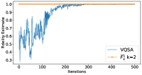
(a) Fidelity of separability calculated for a random product state using the local reward function of the VQSA and benchmarked by $\widetilde{F}_{s}^{1}$.

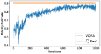
(b) Fidelity of separability calculated for a random entangled state using the local reward function of the VQSA and benchmarked by $\widetilde{F}_{s}^{1}$.

Figure 9: Fidelity of separability estimated using the local reward function of the VQSA and benchmarked by $\widetilde{F}_{s}^{1}$.

Here, in Figure 9(a), we report simulation results after generating a random bipartite product state, with each partition containing two qubits, and calculating the fidelity of separability using both the local reward function of the VQSA and the benchmark $\widetilde{F}^{1}_{s}$, the latter discussed in Appendix E. In Figure 9(b), we do the same for a random bipartite state with the partitions $A$ and $B$ containing two qubits and one qubit, respectively, and three qubits in the reference system. All random states are generated using the hardware efficient ansatz (HEA) [88]. The local reward function of the VQSA requires more classical processing (like picking a qubit at random to measure) and seems to require more iterations to reach the right value. However, these downsides are outweighed by the fact that it is less susceptible to the emergence of barren plateaus.

Appendix H Software

All of our Python source files are available with the arXiv posting of this paper. We performed all simulations using the noisy Qiskit Aer simulator. The Picos Python package [89] was used to invoke the CVXOPT solver [90] for solving the SDPs and the toqito Python package [91] was used for carrying out specific operations on the matrices representing quantum systems.

Appendix I Multipartite Scenarios

In this appendix, we discuss a multipartite generalization of the tests of separability of mixed states.

Definition 8

A state $\rho_{A_{1}\cdots A_{M}}\in\mathcal{D}(\mathcal{H}_{A_{1}\cdots A_{M}})=\mathcal{D}(\mathcal{H}_{A_{1}}\otimes\cdots\otimes\mathcal{H}_{A_{M}})$ is separable if it can be written as

$$\rho_{A_{1}\cdots A_{M}}=\sum_{x\in\mathcal{X}}p(x)\psi^{x,1}_{A_{1}}\otimes\cdots\otimes\psi^{x,M}_{A_{M}},$$ (90)

where $\psi_{A_{i}}^{x,i}$ is a pure state for every $x\in\mathcal{X}$ and $i\in\{1,\ldots,M\}$.

Let $M\text{-SEP}$ denote the set of all $\rho_{A_{1}\cdots A_{M}}\in\mathcal{D}(\mathcal{H}_{A_{1}\cdots A_{M}})$ such that $\rho_{A_{1}\cdots A_{M}}$ is separable. The following theorem is important for the rest of this analysis.

Theorem 9 ([63])

The following formula holds

$$\max_{\sigma_{A_{1}\cdots A_{M}}\in M-\operatorname{SEP}}F(\rho_{A_{1}\cdots A_{M}},\sigma_{A_{1}\cdots A_{M}})=\max_{\{(q(x),\varphi_{A_{1}\cdots A_{M}}^{x})\}_{x}}\sum_{x}q(x)F_{s}(\varphi^{x}_{A_{1}\cdots A_{M}}),$$ (91)

where the optimization is over every pure-state decomposition $\{(q(x),\varphi_{A_{1}\cdots A_{M}}^{x})\}_{x}$ of $\rho_{A_{1}\cdots A_{M}}$ (similar to those in Theorem 4) and

$$F_{s}(\varphi_{A_{1}\cdots A_{M}}^{x})=\max_{\left\{|\phi^{x,i}\rangle_{A_{i}}\right\}_{i=1}^{M}}\left|\langle\varphi^{x}|_{A_{1}\cdots A_{M}}|\phi^{x,1}\rangle_{A_{1}}\otimes\cdots\otimes|\phi^{x,M}\rangle_{A_{M}}\right|^{2}.$$ (92)

For the multipartite case of the distributed quantum computation, the verifier prepares a purification $\psi^{\rho}_{R^{\prime}A_{1}\cdots A_{M}}$ of $\rho_{A_{1}\cdots A_{M}}$. The prover applies a multipartite entanglement-breaking channel on system $R$, which can be written as:

$$\mathcal{E}_{R\rightarrow A^{\prime}_{1}\cdots A^{\prime}_{M-1}}(\cdot)=\sum_{x}\operatorname{Tr}[\mu^{x}_{R}(\cdot)]\left(\phi^{x,1}_{A^{\prime}_{1}}\otimes\cdots\otimes\phi^{x,M-1}_{A^{\prime}_{M-1}}\right),$$ (93)

where $\{\mu^{x}_{R}\}_{x}$ is a rank-one POVM and $\{\phi^{x,i}_{A^{\prime}_{i}}\}_{x,i}$ is a set of pure states. The prover sends systems $(A^{M-1})^{\prime}\equiv A^{\prime}_{1}\cdots A^{\prime}_{M-1}$ to the verifier. Now, the verifier performs a collective swap test of these systems with $A_{1}\cdots A_{M}$, as depicted in Figure 10. The acceptance probability of this distributed quantum computation is given by

$$\max_{\mathcal{E}\in\operatorname{EB}_{M-1}}\operatorname{Tr}[\Pi_{(A^{M-1})^{\prime}A^{M-1}}^{\operatorname{sym}}\mathcal{E}_{R\rightarrow(A^{M-1})^{\prime}}(\psi_{RA^{M-1}})],$$ (94)

where $\mathcal{E}\in\operatorname{EB}_{M-1}$ denotes the set of entanglement-breaking channels defined in (93). This leads to the following theorem:

Theorem 10

For a pure state $\psi_{RA^{M}}\equiv\psi_{RA_{1}\cdots A_{M}}$, the following equality holds:

$$\max_{\mathcal{E}\in\operatorname{EB}_{M-1}}\operatorname{Tr}[\Pi_{(A^{M-1})^{\prime}(A^{M-1})}^{\operatorname{sym}}\mathcal{E}_{R\rightarrow A^{\prime}_{1}\cdots A^{\prime}_{M-1}}(\psi_{RA^{M}})]=\frac{1}{2}\left(1+\max_{\sigma_{A_{1}\cdots A_{M}}\in M-\operatorname{SEP}}F(\rho_{A_{1}\cdots A_{M}},\sigma_{A_{1}\cdots A_{M}})\right).$$ (95)

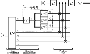
Figure 10: Test for separability of multipartite mixed states. The verifier uses a unitary circuit $U^{\rho}$ to produce the state $\psi_{RA_{1}A_{2}A_{3}A_{4}}$, which is a purification of $\rho_{A_{1}A_{2}A_{3}A_{4}}$. The prover (indicated by the dotted box) applies an entanglement-breaking channel $\mathcal{E}_{R\rightarrow A^{\prime}_{1}A^{\prime}_{2}A^{\prime}_{3}}$ on $R$ by measuring the rank-one POVM $\{\mu^{x}_{R}\}_{x}$ and then, depending on the outcome $x$, prepares a state from the set $\{\phi^{x,1}_{A^{\prime}_{1}}\otimes\phi^{x,2}_{A^{\prime}_{2}}\otimes\phi^{x,3}_{A^{\prime}_{3}}\}_{x}$. The final state is sent to the verifier, who performs a collective swap test. Theorem 10 states that the maximum acceptance probability of this interactive proof is equal to $\frac{1}{2}(1+F_{s}(\rho_{A_{1}A_{2}A_{3}A_{4}}))$, i.e., a simple function of the multipartite fidelity of separability.

Proof. The circuit diagram is given in Figure 10. The verifier prepares a purification $\psi^{\rho}_{R^{\prime}A_{1}\cdots A_{M}}$ of $\rho_{A_{1}\cdots A_{M}}$. The prover applies a multipartite entanglement-breaking channel on $R$, which can be written as:

$$\mathcal{E}_{R\rightarrow A^{\prime}_{1}\cdots A^{\prime}_{M-1}}(\cdot)=\sum_{x}\operatorname{Tr}[\mu^{x}_{R}(\cdot)]\left(\phi^{x,1}_{A^{\prime}_{1}}\otimes\cdots\otimes\phi^{x,M-1}_{A^{\prime}_{M-1}}\right),$$ (96)

where $\{\mu^{x}_{R}\}_{x}$ is a rank-one POVM and $\{\phi^{x,i}_{A^{\prime}_{i}}\}_{x,i}$ is a set of pure states. The prover sends the systems $(A^{M-1})^{\prime}=A^{\prime}_{1}\cdots A^{\prime}_{M-1}$ to the verifier. Now, the verifier performs a collective swap test on $A_{1}\cdots A_{M}$, as depicted at the final part of the circuit diagram in Figure 10. The acceptance probability of this interactive proof system is thus given by

$$\max_{\mathcal{E}\in\text{EB}}\operatorname{Tr}[\Pi_{(A_{1}\cdots A_{M-1})^{\prime}A_{1}\cdots A_{M-1}}^{\text{sym}}\mathcal{E}_{R\rightarrow(A_{1}\cdots A_{M-1})^{\prime}}(\psi_{RA_{1}\cdots A_{M}})],$$ (97)

where

$$\Pi^{\text{sym}}_{(A_{1}\cdots A_{M-1})^{\prime}A_{1}\cdots A_{M-1}}:=\frac{I_{(A_{1}\cdots A_{M-1})^{\prime}A_{1}\cdots A_{M-1}}+F_{(A_{1}\cdots A_{M-1})^{\prime}A_{1}\cdots A_{M-1}}}{2}$$ (98)

is the projector onto the symmetric subspace of $A^{\prime}$ and $A$ and $F_{(A_{1}\cdots A_{M-1})^{\prime}A_{1}\cdots A_{M-1}}$ is a tensor product of individual swaps $F_{A^{\prime}_{i}A_{i}}$, for $i\in\{1,\ldots,M\}$. That is,

$$F_{(A_{1}\cdots A_{M-1})^{\prime}A_{1}\cdots A_{M-1}}=\bigotimes_{i=1}^{n}F_{A^{\prime}_{i}A_{i}}.$$ (99)

Then we find, for fixed $\mathcal{E}_{R\rightarrow A^{\prime}_{1}\cdots A^{\prime}_{M-1}}$, that

$$\operatorname{Tr}[\Pi_{(A_{1}\cdots A_{M-1})^{\prime}(A_{1}\cdots A_{M-1})}^{\text{sym}}\mathcal{E}_{R\rightarrow A^{\prime}_{1}\cdots A^{\prime}_{M-1}}(\psi_{RA_{1}\cdots A_{M}})]$$

$$=\frac{1}{2}\operatorname{Tr}[(I_{(A_{1}\cdots A_{M-1})^{\prime}(A_{1}\cdots A_{M-1})}+F_{(A_{1}\cdots A_{M-1})^{\prime}(A_{1}\cdots A_{M-1})})\mathcal{E}_{R\rightarrow A^{\prime}_{1}\cdots A^{\prime}_{M-1}}(\psi_{RA_{1}\cdots A_{M}})]$$ (100)

$$=\frac{1}{2}+\frac{1}{2}\operatorname{Tr}[(F_{(A_{1}\cdots A_{M-1})^{\prime}(A_{1}\cdots A_{M-1})})\mathcal{E}_{R\rightarrow A^{\prime}_{1}\cdots A^{\prime}_{M-1}}(\psi_{RA^{M}})]$$ (101)

$$=\frac{1}{2}+\frac{1}{2}\operatorname{Tr}[(F_{(A_{1}\cdots A_{M-1})^{\prime}(A_{1}\cdots A_{M-1})})\sum_{x}\operatorname{Tr}[\mu^{x}_{R}(\psi_{RA^{M}})]\phi^{x,1}_{A^{\prime}_{1}}\otimes\cdots\otimes\phi^{x,M-1}_{A^{\prime}_{M-1}}],$$ (102)

$$=\frac{1}{2}+\frac{1}{2}\operatorname{Tr}[(F_{(A_{1}\cdots A_{M-1})^{\prime}(A_{1}\cdots A_{M-1})})\sum_{x}p(x)(\psi^{x}_{A_{1}\cdots A_{M}})\phi^{x,1}_{A^{\prime}_{1}}\otimes\cdots\otimes\phi^{x,M-1}_{A^{\prime}_{M-1}}],$$ (103)

$$=\frac{1}{2}+\frac{1}{2}\sum_{x}p(x)\operatorname{Tr}\!\left[\left(\phi^{x,1}_{A_{1}}\otimes\cdots\otimes\phi^{x,M-1}_{A_{M-1}}\right)\psi^{x}_{A_{1}\cdots A_{M-1}}\right],$$ (104)

where

$$p(x) \coloneqq\operatorname{Tr}[\mu^{x}_{R}(\psi_{RA^{M}})],$$ (105)

$$\psi^{x}_{A_{1}\cdots A_{M}} \coloneqq\frac{1}{p(x)}\operatorname{Tr}_{R}[\mu^{x}_{R}(\psi_{RA^{M}})].$$ (106)

For a given $x$, let us simplify $F_{s}(\varphi_{A_{1}\cdots A_{M}})$ as defined in (92),

$$F_{s}(\varphi_{A_{1}\cdots A_{M}}) =\max_{\left\{|\phi^{i}\rangle_{A_{i}}\right\}_{i=1}^{M}}\left|\langle\varphi|_{A_{1}\cdots A_{M}}|\phi^{1}\rangle_{A_{1}}\otimes\cdots\otimes|\phi^{M}\rangle_{A_{M}}\right|^{2}$$ (107)

$$=\max_{\left\{|\phi^{i}\rangle_{A_{i}}\right\}_{i=1}^{M}}\left|\langle\phi^{1}|_{A_{1}}\otimes\cdots\otimes\langle\phi^{M}|_{A_{M}}|\varphi\rangle_{A_{1}\cdots A_{M}}\right|^{2}$$ (108)

$$=\max_{\left\{|\phi^{i}\rangle_{A_{i}}\right\}_{i=1}^{M-1}}\left\|\langle\phi^{1}|_{A_{1}}\otimes\cdots\otimes\langle\phi^{M-1}|_{A_{M-1}}\otimes I_{A_{M}}|\varphi\rangle_{A^{M}}\right\|_{2}^{2}$$ (109)

$$=\max_{\left\{|\phi^{i}\rangle_{A_{i}}\right\}_{i=1}^{M-1}}\operatorname{Tr}[(|\phi^{1}\rangle\!\langle\phi^{1}|_{A_{1}}\otimes\cdots\otimes|\phi^{M-1}\rangle\!\langle\phi^{M-1}|_{A_{M-1}}\otimes I_{A_{M}})\varphi_{A_{1}\cdots A_{M}}]$$ (110)

$$=\max_{\left\{|\phi^{i}\rangle_{A_{i}}\right\}_{i=1}^{M-1}}\operatorname{Tr}[(|\phi^{1}\rangle\!\langle\phi^{1}|_{A_{1}}\otimes\cdots\otimes|\phi^{M-1}\rangle\!\langle\phi^{M-1}|_{A_{M-1}})\varphi_{A_{1}\cdots A_{M-1}}].$$ (111)

The first two equalities are from the definition and a rewriting. The third equality follows from the variational characterization of the Euclidean norm of a vector. Noting the form in (111) and applying the maximization over entanglement-breaking channels of the form described in (93) to (104), we arrive at the desired claim in (95).   

Figure 11: VQSA to estimate the multipartite fidelity of separability $F_{s}(\rho_{A_{1}A_{2}A_{3}A_{4}})$. The unitary circuit $U^{\rho}$ prepares the state $\psi_{RA_{1}A_{2}A_{3}A_{4}}$, which is a purification of $\rho_{A_{1}A_{2}A_{3}A_{4}}$. The parameterized circuit $W_{R}(\Theta)$ acts on $R$ to evolve the state to another purification of $\rho_{A_{1}A_{2}A_{3}A_{4}}$. The measurement that follows, labeled “steering measurement,” steers the remaining systems to be in a state $\psi_{A_{1}A_{2}A_{3}A_{4}}^{x}$ if the measurement outcome $x$ occurs. Conditioned on the outcome $x$, the final parameterized circuits $U^{x,1}_{A_{1}}(\Theta^{x}_{1})$, $U^{x,2}_{A_{2}}(\Theta^{x}_{2})$, and $U^{x,3}_{A_{3}}(\Theta^{x}_{3})$ are applied and the subsequent measurement estimates the quantity $\operatorname{Tr}\!\left[\left(\phi^{x,1}_{A_{1}}\otimes\phi^{x,2}_{A_{2}}\otimes\phi^{x,3}_{A_{3}}\right)\psi^{x}_{A_{1}A_{2}A_{3}}\right]$.

We can then use the generalized test of separability of mixed states to develop a VQSA for the multipartite case. See Figure 11. This involves replacing the collective swap test in Figure 10 with an overlap measurement, similar to how we got Figure 2 in the main text from Figure 1 in the main text.

Appendix J Complexity Class QIP${}_{\operatorname{EB}}(2)$

In this appendix, we establish a complete problem for QIP${}_{\operatorname{EB}}(2)$, and then we interpret this problem in Remark 12. Let us first define the complexity class QIP${}_{\operatorname{EB}}(2)$. Let $A=\left(A_{\text{yes}},A_{\text{no}}\right)$ be a promise problem and let $a,b:\mathbb{N}\to[0,1]$ and $p$ be polynomial functions. The verifier $V$ is described by a polynomial-time generated family of quantum circuits. The prover $P$ is a family of arbitrary entanglement-breaking channels that interface with a given verifier in a natural way. Then $A\in$ QIP${}_{\operatorname{EB}}(2)$$(a,b)$ if there exists a two-message verifier with the following properties:

1. Completeness: For all $x\in A_{\text{yes}}$, there exists a prover $P$ that causes the verifier $V$ to accept $x$ with probability at least $a(|x|)$.

2. Soundness: For all $x\in A_{\text{no}}$, every prover $P$ that causes the verifier $V$ to accept $x$ with probability at most $b(|x|)$.

In the above, acceptance is defined as obtaining the outcome one upon measuring the decision-qubit register.

Theorem 11

Given a circuit to generate a channel $\mathcal{N}_{G\rightarrow S}$ and a state $\rho_{S}$, estimating the following quantity within additive error $\varepsilon\in(0,1)$ is a complete problem for $\operatorname{QIP}_{\operatorname{EB}}(2)$:

$$\max_{\begin{subarray}{c}\{(p(x),\psi^{x})\}_{x},\\ \left\{\varphi^{x}\right\}_{x},\\ \sum_{x}p(x)\psi_{S}^{x}=\rho_{S}\end{subarray}}\sum_{x}p(x)F(\psi_{S}^{x},\mathcal{N}_{G\rightarrow S}(\varphi_{G}^{x})),$$ (112)

where the optimization is over every pure-state decomposition of $\rho_{S}$, as $\sum_{x}p(x)\psi_{S}^{x}=\rho_{S}$, and $\left\{\varphi^{x}\right\}_{x}$ is a set of pure states.

Proof. Consider a general interactive proof system in QIP${}_{\operatorname{EB}}(2)$ that begins with the verifier preparing a bipartite pure state $\psi_{RS}$, followed by the system $R$ being sent to the prover, who subsequently performs an entanglement-breaking channel. The verifier then performs a unitary $V_{R^{\prime}S\rightarrow DG}$ and projects onto the $|1\rangle\!\langle 1|$ state of the decision qubit. Indeed, the acceptance probability is given by

$$\max_{\mathcal{E}\in\operatorname{EB}}\operatorname{Tr}[(|1\rangle\!\langle 1|_{D}\otimes I_{G})\mathcal{V}_{R^{\prime}S\rightarrow DG}(\mathcal{E}_{R\rightarrow R^{\prime}}(\psi_{RS}))],$$ (113)

where $\mathcal{V}_{R^{\prime}S\rightarrow DG}$ is the unitary channel corresponding to the unitary operator $V_{R^{\prime}S\rightarrow DG}$. By previous reasoning, we find that

$$\mathcal{E}_{R\rightarrow R^{\prime}}(\psi_{RS})=\sum_{x}p(x)\phi_{R^{\prime}}^{x}\otimes\psi_{S}^{x},$$ (114)

so that the acceptance probability is equal to

$$\max_{\begin{subarray}{c}\{(p(x),\psi^{x})\}_{x},\\ \left\{\phi^{x}\right\}_{x},\\ \sum_{x}p(x)\psi_{S}^{x}=\psi_{S}\end{subarray}}\operatorname{Tr}\!\left[(|1\rangle\!\langle 1|_{D}\otimes I_{G})\mathcal{V}\left(\sum_{x}p(x)\phi_{R^{\prime}}^{x}\otimes\psi_{S}^{x}\right)\right]\\ =\max_{\begin{subarray}{c}\{(p(x),\psi^{x})\}_{x},\\ \left\{\phi^{x}\right\}_{x},\\ \sum_{x}p(x)\psi_{S}^{x}=\psi_{S}\end{subarray}}\sum_{x}p(x)\operatorname{Tr}\!\left[(|1\rangle\!\langle 1|_{D}\otimes I_{G})\mathcal{V}\left(\phi_{R^{\prime}}^{x}\otimes\psi_{S}^{x}\right)\right],$$ (115)

where we have used the shorthand $\mathcal{V}\equiv\mathcal{V}_{R^{\prime}S\rightarrow DG}$. Consider that

$$\operatorname{Tr}\!\left[(|1\rangle\!\langle 1|_{D}\otimes I_{G})\mathcal{V}\left(\phi_{R^{\prime}}^{x}\otimes\psi_{S}^{x}\right)\right] =\left\|\langle 1|_{D}\otimes I_{G})V|\phi^{x}\rangle_{R^{\prime}}\otimes|\psi^{x}\rangle_{S}\right\|_{2}^{2}$$ (116)

$$=\max_{|\varphi^{x}\rangle_{G}}\left|\langle 1|_{D}\otimes\langle\varphi^{x}|_{G})V|\phi^{x}\rangle_{R^{\prime}}\otimes|\psi^{x}\rangle_{S}\right|^{2}$$ (117)

$$=\max_{|\varphi^{x}\rangle_{G}}\operatorname{Tr}\!\left[V^{{\dagger}}(|1\rangle\!\langle 1|_{D}\otimes|\varphi^{x}\rangle\!\langle\varphi^{x}|_{G})V\phi^{x}_{R^{\prime}}\otimes|\psi^{x}\rangle\!\langle\psi^{x}|_{S}\right]$$ (118)

$$=\max_{|\varphi^{x}\rangle_{G}}\operatorname{Tr}\!\left[\mathcal{W}_{G\rightarrow R^{\prime}S}(|\varphi^{x}\rangle\!\langle\varphi^{x}|_{G})\phi^{x}_{R^{\prime}}\otimes|\psi^{x}\rangle\!\langle\psi^{x}|_{S}\right],$$ (119)

where the isometric channel $\mathcal{W}_{G\to R^{\prime}S}$ is defined as

$$\mathcal{W}_{G\rightarrow R^{\prime}S}(\cdot)\coloneqq(V_{R^{\prime}S\rightarrow DG})^{{\dagger}}(|1\rangle\!\langle 1|_{D}\otimes(\cdot)_{G})V_{R^{\prime}S\rightarrow DG}.$$ (120)

Then the acceptance probability is given by

$$\max_{\begin{subarray}{c}\{(p(x),\psi^{x})\}_{x},\\ \left\{\phi^{x}\right\}_{x},\left\{\varphi^{x}\right\}_{x}\end{subarray}}\left\{\begin{array}[c]{c}\sum_{x}p(x)\operatorname{Tr}\!\left[\mathcal{W}_{G\rightarrow R^{\prime}S}(|\varphi^{x}\rangle\!\langle\varphi^{x}|_{G})\phi^{x}_{R^{\prime}}\otimes|\psi^{x}\rangle\!\langle\psi^{x}|_{S}\right]:\\ \sum_{x}p(x)\psi_{S}^{x}=\psi_{S}\end{array}\right\}.$$ (121)

Since the optimization over $\phi^{x}_{R^{\prime}}$ is arbitrary, we can also write

$$\max_{|\phi^{x}\rangle_{R^{\prime}}}\operatorname{Tr}\!\left[\mathcal{W}_{G\rightarrow R^{\prime}S}(|\varphi^{x}\rangle\!\langle\varphi^{x}|_{G})\phi^{x}_{R^{\prime}}\otimes|\psi^{x}\rangle\!\langle\psi^{x}|_{S}\right]$$

$$=\max_{|\phi^{x}\rangle_{R^{\prime}}}\left|\langle\phi^{x}|_{R^{\prime}}\otimes\langle\psi^{x}|_{S}W_{G\rightarrow R^{\prime}S}|\varphi^{x}\rangle_{G}\right|^{2}$$

$$=\left\|I_{R^{\prime}}\otimes\langle\psi^{x}|_{S}W_{G\rightarrow R^{\prime}S}|\varphi^{x}\rangle_{G}\right\|_{2}^{2}$$

$$=\left(\langle\varphi^{x}|_{G}\left(W_{G\rightarrow R^{\prime}S}\right)^{{\dagger}}I_{R^{\prime}}\otimes|\psi^{x}\rangle_{S}\right)\left(I_{R^{\prime}}\otimes\langle\psi^{x}|_{S}W_{G\rightarrow R^{\prime}S}|\varphi^{x}\rangle_{G}\right)$$

$$=\langle\varphi^{x}|_{G}\left(W_{G\rightarrow R^{\prime}S}\right)^{{\dagger}}\left(I_{R^{\prime}}\otimes|\psi^{x}\rangle\!\langle\psi^{x}|_{S}\right)W_{G\rightarrow R^{\prime}S}|\varphi^{x}\rangle_{G}$$

$$=\operatorname{Tr}\!\left[\left(I_{R^{\prime}}\otimes|\psi^{x}\rangle\!\langle\psi^{x}|_{S}\right)W_{G\rightarrow R^{\prime}S}|\varphi^{x}\rangle\!\langle\varphi^{x}|_{G}\left(W_{G\rightarrow R^{\prime}S}\right)^{{\dagger}}\right]$$

$$=\operatorname{Tr}[|\psi^{x}\rangle\!\langle\psi^{x}|_{S}\mathcal{N}_{G\rightarrow S}(|\varphi^{x}\rangle\!\langle\varphi^{x}|_{G})],$$ (122)

where we define the channel $\mathcal{N}_{G\rightarrow S}$ as

$$\mathcal{N}_{G\rightarrow S}(\cdot)\coloneqq\operatorname{Tr}_{R^{\prime}}[(V_{R^{\prime}S\rightarrow DG})^{{\dagger}}(|1\rangle\!\langle 1|_{D}\otimes(\cdot)_{G})V_{R^{\prime}S\rightarrow DG}].$$ (123)

Then we find that the acceptance probability is given by

$$\max_{\begin{subarray}{c}\{(p(x),\psi^{x})\}_{x},\\ \left\{\varphi^{x}\right\}_{x},\\ \sum_{x}p(x)\psi_{S}^{x}=\psi_{S}\end{subarray}}\sum_{x}p(x)\operatorname{Tr}[|\psi^{x}\rangle\!\langle\psi^{x}|_{S}\mathcal{N}_{G\rightarrow S}(|\varphi^{x}\rangle\!\langle\varphi^{x}|_{G})]=\max_{\begin{subarray}{c}\{(p(x),\psi^{x})\}_{x},\left\{\varphi^{x}\right\}_{x}\\ \sum_{x}p(x)\psi_{S}^{x}=\psi_{S}\end{subarray}}\sum_{x}p(x)F(\psi_{S}^{x},\mathcal{N}_{G\rightarrow S}(\varphi_{G}^{x})).$$ (124)

This concludes the proof.   

Remark 12

The quantity in (112) can be interpreted as follows: Given a channel $\mathcal{N}$ and a source $\rho$, calculate the largest average ensemble fidelity attainable in reproducing the source at the output of the channel. This means it is necessary to find the ensemble decomposition $\{(p(x),\psi^{x})\}_{x}$ of $\rho$ as well as a set $\left\{\varphi^{x}\right\}_{x}$ of encoding states that lead to the largest ensemble fidelity (and this is what is left to the prover). This criterion is similar to one that is used in Schumacher data compression [92], but this seems more similar to the setting of the source-channel separation theorem [93], in which the goal is to transmit an information source over a quantum channel. The channel $\mathcal{N}$ here could consist of a fixed encoding $\mathcal{E}$, noisy channel $\mathcal{M}$, and fixed decoding $\mathcal{D}$, (i.e., $\mathcal{N}=\mathcal{D}\circ\mathcal{M}\circ\mathcal{E}$) and then the goal is to test how well a given fixed scheme $(\mathcal{E},\mathcal{D})$ can communicate a source $\rho$ over a channel $\mathcal{M}$, according to the ensemble fidelity criterion.

Remark 13

We can write the expression in (112) alternatively as

$$\text{\rm Eq.\leavevmode\nobreak\ \eqref{eq:accept-prob-qip_eb-2}}=\max_{\begin{subarray}{c}\{(p(x),\psi^{x})\}_{x},\\ \sum_{x}p(x)\psi_{S}^{x}=\rho_{S}\end{subarray}}\sum_{x}p(x)\left\|(\mathcal{N}_{G\rightarrow S})^{{\dagger}}(\psi_{S}^{x})\right\|_{\infty},$$ (125)

where $(\mathcal{N}_{G\rightarrow S})^{{\dagger}}$ is the Hilbert–Schmidt adjoint of the channel $(\mathcal{N}_{G\rightarrow S})^{{\dagger}}$. Employing the abbreviations $\psi^{x}_{S}\equiv|\psi^{x}\rangle\!\langle\psi^{x}|_{S}$ and $\varphi^{x}_{G}\equiv|\varphi^{x}\rangle\!\langle\varphi^{x}|_{G}$, this follows because

$$\max_{\begin{subarray}{c}\{(p(x),\psi^{x})\}_{x},\\ \left\{\varphi^{x}\right\}_{x},\\ \sum_{x}p(x)\psi_{S}^{x}=\psi_{S}\end{subarray}}\sum_{x}p(x)\operatorname{Tr}[\psi^{x}_{S}\mathcal{N}_{G\rightarrow S}(\varphi^{x}_{G})]$$

$$=\max_{\begin{subarray}{c}\{(p(x),\psi^{x})\}_{x},\\ \left\{\varphi^{x}\right\}_{x},\\ \sum_{x}p(x)\psi_{S}^{x}=\psi_{S}\end{subarray}}\sum_{x}p(x)\operatorname{Tr}[(\mathcal{N}_{G\rightarrow S})^{{\dagger}}(\psi^{x}_{S})\varphi^{x}_{G}]$$ (126)

$$=\max_{\begin{subarray}{c}\{(p(x),\psi^{x})\}_{x},\\ \left\{\varphi^{x}\right\}_{x},\\ \sum_{x}p(x)\psi_{S}^{x}=\psi_{S}\end{subarray}}\sum_{x}p(x)\max_{\left\{\varphi^{x}\right\}_{x}}\operatorname{Tr}[(\mathcal{N}_{G\rightarrow S})^{{\dagger}}(\psi^{x}_{S})\varphi^{x}_{G}]$$ (127)

$$=\max_{\begin{subarray}{c}\{(p(x),\psi^{x})\}_{x},\\ \sum_{x}p(x)\psi_{S}^{x}=\rho_{S}\end{subarray}}\sum_{x}p(x)\left\|(\mathcal{N}_{G\rightarrow S})^{{\dagger}}(\psi_{S}^{x})\right\|_{\infty}.$$ (128)

If we define the function

$$g_{\mathcal{N}}(\rho)\coloneqq\left\|(\mathcal{N}_{G\rightarrow S})^{{\dagger}}(\rho_{S})\right\|_{\infty},$$ (129)

then the function in (125) is known as the concave closure of $g_{\mathcal{N}}(\rho)$ and has been studied in other contexts in quantum information theory [94, Section 2]. It has an interesting dual formulation, as demonstrated in [94, Eq. (15)]. Given the observation in (125), we can thus conclude that, given circuits to realize the channel $\mathcal{N}$ and state $\rho$, estimating the concave closure of the function $g_{\mathcal{N}}(\rho)$ within additive error is a complete problem for QIP${}_{\operatorname{EB}}(2)$.

Remark 14

Employing the reasoning from Remark 13, we find that the acceptance probability in (33) is equal to the concave closure of the following function:

$$f(\rho_{AB})\coloneqq\left\|\Pi^{\operatorname{sym}}_{AA^{\prime}}(\rho_{AB}\otimes I_{A^{\prime}})\Pi^{\operatorname{sym}}_{AA^{\prime}}\right\|_{\infty},$$ (130)

where we used the fact that the state $\rho_{S}$ from Remark 13 is $\rho_{AB}$ and the map $\mathcal{N}_{G\to S}$ from Remark 13 is

$$\mathcal{N}(\sigma_{AA^{\prime}B})=\operatorname{Tr}_{A^{\prime}}[\Pi^{\operatorname{sym}}_{AA^{\prime}}\sigma_{AA^{\prime}B}\Pi^{\operatorname{sym}}_{AA^{\prime}}],$$ (131)

with adjoint

$$\mathcal{N}^{{\dagger}}(\omega_{AB})=\Pi^{\operatorname{sym}}_{AA^{\prime}}(\omega_{AB}\otimes I_{A^{\prime}})\Pi^{\operatorname{sym}}_{AA^{\prime}}.$$ (132)

Observe that the map $\rho_{AB}\mapsto\Pi^{\operatorname{sym}}_{AA^{\prime}}(\rho_{AB}\otimes I_{A^{\prime}})\Pi^{\operatorname{sym}}_{AA^{\prime}}$ is proportional to that used in a $1\to 2$ universal cloning machine [95, Eq. (17)]. If $\rho_{AB}$ is pure, so that we write it as $\psi_{AB}$, then the following inequality holds:

$$\left\|\Pi^{\operatorname{sym}}_{AA^{\prime}}(\psi_{AB}\otimes I_{A^{\prime}})\Pi^{\operatorname{sym}}_{AA^{\prime}}\right\|_{\infty}\leq\left\|\Pi^{\operatorname{sym}}_{AA^{\prime}}\right\|_{\infty}\left\|\psi_{AB}\otimes I_{A^{\prime}}\right\|_{\infty}\left\|\Pi^{\operatorname{sym}}_{AA^{\prime}}\right\|_{\infty}\leq 1,$$ (133)

where we applied the multiplicativity of the spectral norm. Thus, the concave closure of $f(\rho_{AB})$ satisfies $f(\rho_{AB})\in[0,1]$. Furthermore, from Lemma 15 below, we know that

$$\left\|\Pi^{\operatorname{sym}}_{AA^{\prime}}(\psi_{AB}\otimes I_{A^{\prime}})\Pi^{\operatorname{sym}}_{AA^{\prime}}\right\|_{\infty}=\frac{1}{2}\left(1+\left\|\psi_{A}\right\|_{\infty}\right),$$ (134)

showing the consistency of the claim just above (130) with Theorem 1 and Eqs. (17) and (18) in the main text. If $\rho_{AB}$ is a pure product state, so that we can write it as $\rho_{AB}=\phi_{A}\otimes\varphi_{B}$, then we have that

$$\left\|\Pi^{\operatorname{sym}}_{AA^{\prime}}(\phi_{A}\otimes\varphi_{B}\otimes I_{A^{\prime}})\Pi^{\operatorname{sym}}_{AA^{\prime}}\right\|_{\infty}=\left\|\Pi^{\operatorname{sym}}_{AA^{\prime}}(\phi_{A}\otimes I_{A^{\prime}})\Pi^{\operatorname{sym}}_{AA^{\prime}}\right\|_{\infty},$$ (135)

and the spectral norm on the right-hand side of (135) is achieved by choosing the vector $|\phi\rangle_{A}\otimes|\phi\rangle_{A^{\prime}}$, so that

$$(\langle\phi|_{A}\otimes\langle\phi|_{A^{\prime}})\Pi^{\operatorname{sym}}_{AA^{\prime}}(\phi_{A}\otimes I_{A^{\prime}})\Pi^{\operatorname{sym}}_{AA^{\prime}}(|\phi\rangle_{A}\otimes|\phi\rangle_{A^{\prime}})$$

$$=(\langle\phi|_{A}\otimes\langle\phi|_{A^{\prime}})(\phi_{A}\otimes I_{A^{\prime}})(|\phi\rangle_{A}\otimes|\phi\rangle_{A^{\prime}})$$ (136)

$$=1.$$ (137)

Lemma 15

For a pure state $\psi_{AB}$, the following equality holds:

$$\left\|\Pi^{\operatorname{sym}}_{AA^{\prime}}(\psi_{AB}\otimes I_{A^{\prime}})\Pi^{\operatorname{sym}}_{AA^{\prime}}\right\|_{\infty}=\frac{1}{2}\left(1+\left\|\psi_{A}\right\|_{\infty}\right),$$ (138)

where $\psi_{A}\equiv\operatorname{Tr}_{B}[\psi_{AB}]$.

Proof. Consider that

$$\left\|\left(\Pi_{AA^{\prime}}^{\text{sym}}\otimes I_{B}\right)\left(|\psi\rangle\!\langle\psi|_{AB}\otimes I_{A^{\prime}}\right)\left(\Pi_{AA^{\prime}}^{\text{sym}}\otimes I_{B}\right)\right\|_{\infty}\\ =\left\|\left(|\psi\rangle\!\langle\psi|_{AB}\otimes I_{A^{\prime}}\right)\left(\Pi_{AA^{\prime}}^{\text{sym}}\otimes I_{B}\right)\left(|\psi\rangle\!\langle\psi|_{AB}\otimes I_{A^{\prime}}\right)\right\|_{\infty}.$$ (139)

Now consider that

$$\left(|\psi\rangle\!\langle\psi|_{AB}\otimes I_{A^{\prime}}\right)\left(\Pi_{AA^{\prime}}^{\text{sym}}\otimes I_{B}\right)\left(|\psi\rangle\!\langle\psi|_{AB}\otimes I_{A^{\prime}}\right)$$

$$=\left(|\psi\rangle\!\langle\psi|_{AB}\otimes I_{A^{\prime}}\right)\left(\frac{I_{AA^{\prime}}+F_{AA^{\prime}}}{2}\otimes I_{B}\right)\left(|\psi\rangle\!\langle\psi|_{AB}\otimes I_{A^{\prime}}\right)$$

$$=\frac{1}{2}\left(|\psi\rangle\!\langle\psi|_{AB}\otimes I_{A^{\prime}}\right)+\frac{1}{2}\left(|\psi\rangle\!\langle\psi|_{AB}\otimes I_{A^{\prime}}\right)\left(F_{AA^{\prime}}\otimes I_{B}\right)\left(|\psi\rangle\!\langle\psi|_{AB}\otimes I_{A^{\prime}}\right).$$ (140)

Then writing the Schmidt decomposition of $|\psi\rangle_{AB}$ as $|\psi\rangle_{AB}=\sum_{i}\sqrt{\lambda_{i}}|i\rangle_{A}|i\rangle_{B}$, we find that

$$\left(|\psi\rangle\!\langle\psi|_{AB}\otimes I_{A^{\prime}}\right)\left(F_{AA^{\prime}}\otimes I_{B}\right)\left(|\psi\rangle\!\langle\psi|_{AB}\otimes I_{A^{\prime}}\right)$$

$$=\sum_{i,i^{\prime},j,j^{\prime}}\sqrt{\lambda_{i}\lambda_{i^{\prime}}}\left(|\psi\rangle\!\langle i|_{A}\langle i|_{B}\otimes|j\rangle\!\langle j|_{A^{\prime}}\right)\left(F_{AA^{\prime}}\otimes I_{B}\right)\left(|i^{\prime}\rangle_{A}|i^{\prime}\rangle_{B}\langle\psi|_{AB}\otimes|j^{\prime}\rangle\!\langle j^{\prime}|_{A^{\prime}}\right)$$ (141)

$$=\sum_{i,i^{\prime},j,j^{\prime}}\sqrt{\lambda_{i}\lambda_{i^{\prime}}}\left(|\psi\rangle\!\langle i|_{A}\langle i|_{B}\otimes|j\rangle\!\langle j|_{A^{\prime}}\right)\left(|j^{\prime}\rangle_{A}|i^{\prime}\rangle_{B}\langle\psi|_{AB}\otimes|i^{\prime}\rangle\!\langle j^{\prime}|_{A^{\prime}}\right)$$ (142)

$$=\sum_{i,i^{\prime},j,j^{\prime}}\sqrt{\lambda_{i}\lambda_{i^{\prime}}}|\psi\rangle\!\langle i|j^{\prime}\rangle_{A}\langle i|i^{\prime}\rangle_{B}\langle\psi|_{AB}\otimes|j\rangle\!\langle j|i^{\prime}\rangle\!\langle j^{\prime}|_{A^{\prime}}$$ (143)

$$=\sum_{i}\lambda_{i}|\psi\rangle\!\langle\psi|_{AB}\otimes|i\rangle\!\langle i|_{A^{\prime}}$$ (144)

$$=|\psi\rangle\!\langle\psi|_{AB}\otimes\sum_{i}\lambda_{i}|i\rangle\!\langle i|_{A^{\prime}}$$ (145)

$$=|\psi\rangle\!\langle\psi|_{AB}\otimes\psi_{A^{\prime}}.$$ (146)

Then

$$\left(|\psi\rangle\!\langle\psi|_{AB}\otimes I_{A^{\prime}}\right)\left(\Pi_{AA^{\prime}}^{\text{sym}}\otimes I_{B}\right)\left(|\psi\rangle\!\langle\psi|_{AB}\otimes I_{A^{\prime}}\right)$$

$$=\frac{1}{2}\left(|\psi\rangle\!\langle\psi|_{AB}\otimes I_{A^{\prime}}\right)+|\psi\rangle\!\langle\psi|_{AB}\otimes\frac{1}{2}\psi_{A^{\prime}}$$ (147)

$$=|\psi\rangle\!\langle\psi|_{AB}\otimes\frac{1}{2}\left(I_{A^{\prime}}+\psi_{A^{\prime}}\right),$$ (148)

and we conclude that

$$\left\|\left(\Pi_{AA^{\prime}}^{\text{sym}}\otimes I_{B}\right)\left(|\psi\rangle\!\langle\psi|_{AB}\otimes I_{A^{\prime}}\right)\left(\Pi_{AA^{\prime}}^{\text{sym}}\otimes I_{B}\right)\right\|_{\infty}$$

$$=\left\||\psi\rangle\!\langle\psi|_{AB}\otimes\frac{1}{2}\left(I_{A^{\prime}}+\psi_{A^{\prime}}\right)\right\|_{\infty}$$ (149)

$$=\frac{1}{2}\left(1+\left\|\psi_{A^{\prime}}\right\|_{\infty}\right)$$ (150)

$$=\frac{1}{2}\left(1+\left\|\psi_{A}\right\|_{\infty}\right).$$ (151)

This concludes the proof.   

Appendix K Placement of QIP${}_{\operatorname{EB}}(2)$

In this appendix, we show the containment of QIP${}_{\operatorname{EB}}(2)$ as follows:

$$\text{QAM},\text{QSZK}\subseteq\text{QIP${}_{\operatorname{EB}}(2)$}\subseteq\text{QIP}.$$ (152)

See Figure 12 for a detailed diagram.

K.1 QAM $\subseteq$ QIP${}_{\operatorname{EB}}(2)$

First, recall that QAM consists of the verifier selecting a classical letter $x$ uniformly at random, sending the choice to the prover, who then sends back a pure state $\psi_{x}$ to the verifier, who finally performs an efficient measurement to decide whether to accept the computation [57]. Note that QAM contains QMA [57].

To see the containment QAM $\subseteq$ QIP${}_{\operatorname{EB}}(2)$, consider that the verifier’s first circuit in QIP${}_{\operatorname{EB}}(2)$ can consist of preparing a random classical bitstring in a system $R$. The verifier sends system $R$ to the prover. Then the prover’s action just amounts to preparing some state that gets sent back to the verifier. The rest of the protocol then simulates a QAM protocol.

Figure 12: Placement of QIP${}_{\operatorname{EB}}(2)$ relative to other known complexity classes. The complexity classes are organized such that if a class is connected to a class above it, the complexity class placed lower is a subset of the class above. For example, QIP${}_{\operatorname{EB}}(2)$ is subset of QIP and QIP${}_{\operatorname{EB}}(2)$ is a superset of both QMA and QAM.

K.2 QSZK $\subseteq$ QIP${}_{\operatorname{EB}}(2)$

Quantum statistical zero-knowledge (QSZK) consists of all problems that can be solved by the interaction between a quantum verifier and a quantum prover, such that the verifier accumulates statistical evidence about the answer to a decision, but does not learn anything other than the answer by interacting with the prover [96, 58]. A complete problem for this class is quantum state distinguishability, in which the goal is to decide whether two states $\rho_{0}$ and $\rho_{1}$, generated by quantum circuits, are far or close in trace distance [96]. This is a nice problem for understanding the basics of the QSZK complexity class: the interaction begins with the verifier picking one of the states uniformly at random, recording the choice as a bit $x$, and then sending the chosen state $\rho_{x}$ to the prover over a quantum channel. The prover can then perform the optimal Helstrom measurement [97, 98] to distinguish the states, which has success probability equal to

$$p_{\text{succ}}\coloneqq\frac{1}{2}\left(1+\frac{1}{2}\left\|\rho_{0}-\rho_{1}\right\|_{1}\right).$$ (153)

The Helstrom measurement leads to a decision bit $y$, which the prover sends back to the verifier over a quantum channel (here actually a single classical bit channel would suffice). The verifier then accepts if $x=y$, and the probability that this happens is equal to $p_{\text{succ}}$. By repeating this protocol a polynomial number of times and invoking the error-reduction protocol from [96], it follows that the verifier can make the completeness and soundness probabilities exponentially close to one and zero, respectively, to have essentially zero error probability in the final decision about whether the states are near or far in trace distance. Finally, the interaction has a “zero knowledge” aspect because the verifier only learns the bit of the prover and does not learn anything about how to actually distinguish the states.

Since quantum state distinguishability is a complete problem for QSZK and it is clear that the interaction described above can be performed in QIP${}_{\operatorname{EB}}(2)$, it follows that QSZK $\subseteq$ QIP${}_{\operatorname{EB}}(2)$.

K.3 QIP${}_{\operatorname{EB}}(2)$ $\subseteq$ QIP

To see the containment QIP${}_{\operatorname{EB}}(2)$ $\subseteq$ QIP, we need to simulate QIP${}_{\operatorname{EB}}(2)$ in QIP. If we can simulate QIP${}_{\operatorname{EB}}(2)$ in QIP(4), then we know from the general result of [56] that QIP(4) = QIP(3) = QIP.

The first step begins with the verifier acting with the first circuit from the original QIP${}_{\operatorname{EB}}(2)$ protocol. Then the verifier sends some of the output qubits to the QIP prover.

Now, we need to simulate a general entanglement-breaking channel from QIP${}_{\operatorname{EB}}(2)$ with, say, $p(n)$ input qubits and $q(n)$ output qubits, where $p(n)$ and $q(n)$ are polynomials in the complexity parameter $n$. What we need is a handle on the size of the classical register in between. In general, this could be arbitrarily large. However, the Choi state of this channel is separable, and the bound $\left|\mathcal{X}\right|\leq\text{rank}(\sigma_{AB})^{2}$ [50] stated in the main text implies that the number of terms in the decomposition need not be any larger than $2^{2p(n)q(n)}$. This means that the classical register for the channel need not be any larger than $2p(n)q(n)$ qubits.

So the rest of the QIP simulation consists of the prover applying a general unitary, sending back $2p(n)q(n)$ qubits, the verifier decohering / measuring these qubits by attaching to each an ancilla in the all-zeros state $|0\rangle\!\langle 0|$, applying CNOTs, and keeping the second qubits in each pair locally. Then the verifier sends the decohered qubits to the prover, who acts with a general unitary, and sends back some of the outputs to the verifier. The verifier then acts with the final unitary from the original QIP${}_{\operatorname{EB}}(2)$ protocol and measures the decision qubit.

This concludes the proof, as all entanglement-breaking channels can be simulated in this way, and the number of classical bits needed in the middle, by the above argument, need not be larger than twice the product of the number of input and output qubits, which is still polynomial in the input length.

K.4 Error Reduction for QIP${}_{\operatorname{EB}}(2)$ via Parallel Repetition

An important question that arises when defining a complexity class is the issue of repetition, since the verifier cannot make a decision from just one trial, but rather needs to accumulate evidence before doing so [41, 42]. For complexity classes like BPP (efficient probabilistic classical computing) or BQP (efficient quantum computing), this issue is a simple matter of repeating the algorithm a sufficient number of times and taking a majority vote of the outcomes. By an application of the Chernoff bound, it follows that a polynomial number of repetitions implies an exponential decrease in the error probability of making an incorrect decision.

This issue becomes more subtle when interacting with a quantum prover, because the prover has the ability to correlate his actions across multiple trials [41, 42]. Thus, when defining the complexity class QIP${}_{\operatorname{EB}}(2)$ and performing a QIP${}_{\operatorname{EB}}(2)$ algorithm multiple times in parallel, this issue arises because the prover can act with a joint entanglement-breaking channel across all of the systems received from the verifier and then return a state that is entangled across all systems for the final measurements of the verifier. Thus, it is necessary to analyze a method for reducing errors in this case.

Fortunately, for the case of analyzing this problem with QIP${}_{\operatorname{EB}}(2)$, we can make direct use of a prior analysis [99, Section 3.2] for the parallel repetition and error reduction for the class QIP(2), essentially verbatim. We note that other approaches for error reduction with QIP(2) are available [100, 101], but we do not make use of them here.

To summarize the idea from [99, Section 3.2], starting from a fixed QIP${}_{\operatorname{EB}}(2)$ protocol, which consists of an initial verifier circuit $V_{1}$, a final verifier circuit $V_{2}$ with a measurement on a single decision qubit, and predetermined bounds $a$ and $b$ on the completeness and soundness probabilities, we define a new QIP${}_{\operatorname{EB}}(2)$ parallelized protocol, which consists of an initial verifier circuit given by $V_{1}^{\otimes st}$ and a final verifier circuit given by $V_{2}^{\otimes st}$, where $s$ and $t$ are positive integers that are no more than polynomial in the problem size. The verifier then receives $st$ measurement outcomes (bits) after measuring all of the decision qubits of $V_{2}^{\otimes st}$ and has to decide whether to accept or reject based on them. The verifier groups the measurement outcomes into $s$ groups of $t$ measurement outcomes each. For the $i$th group, let $z_{i}$ be equal to one if the number of times the protocol accepted in the $i$th group, divided by $t$, is greater than a threshold equal to the average $(a+b)/2$, and let it be equal to zero otherwise. The parallelized verifier then accepts if and only if every $z_{i}$ is equal to one.

By the same analysis given in [99, Section 3.2], if we are in a yes instance in which the verifier should accept, then the prover can act with a tensor product $\mathcal{E}^{\otimes n}$ of the entanglement-breaking channel $\mathcal{E}$ that leads to the highest acceptance probability in an individual trial. By doing so, it then follows from the analysis in [99, Section 3.2] that the acceptance probability of the parallelized protocol in this case is exponentially close to one.

Now consider the case that we are in a no instance in which the verifier should not accept. By the containment QIP${}_{\operatorname{EB}}(2)$ $\subseteq$ QIP discussed in Section K.3, it follows that there is a QIP simulation of the QIP${}_{\operatorname{EB}}(2)$ protocol, with no change in the completeness and soundness probabilities. Thus, following the same reasoning from [99, Section 3.2], the $t$ parallel repetitions of the protocol in the $i$th group (call this the $i$th protocol) can be precisely simulated by a QIP, and the general result from [56] on parallel repetition of QIP applies here. Thus, the acceptance probability of the overall parallelized protocol is no greater than the product of the acceptance probabilities for the individual protocols, and the parameters $s$ and $t$ can be chosen in such a way that the acceptance probability of the overall protocol decays exponentially fast to zero.

Thus, for the parallelized protocol with the classical postprocessing discussed above and with $st$ no more than a polynomial in the problem size, the acceptance probability increases to one exponentially fast in the case of a yes instance, and it decays to zero exponentially fast in the case of a no instance, as desired.

Appendix L Local Reward Function

In this appendix, we develop a local reward function, as an alternative to the global reward function considered in the main text, i.e., the acceptance probability in Theorem 2. The acceptance probability in Theorem 2 can be thought of as a global reward function because it corresponds to the probability of measuring zero in every register. As indicated in [44], it is helpful to employ a local reward function in order to mitigate the barren plateau problem [43], which plagues all variational quantum algorithms.

Let us define the local and global reward functions. To begin, let $Z_{i}$ be the event of measuring zero in the $i$th register. We then set the local reward function to be the probability of measuring zero in a register chosen uniformly at random; that is, it is given by the following:

$$L\equiv\frac{1}{n}\sum_{i}\Pr\!\left(Z_{i}\right).$$ (154)

The event of measuring all zeros is given by $\bigcap_{i}Z_{i}$, and the probability that this event occurs is $G\equiv\Pr\!\left(\bigcap_{i}Z_{i}\right)$, which is what we used in the main text as the global reward function.

Now, we are interested in determining inequalities that relate the global and local reward functions, and the following analysis employs the same ideas used in [82, Appendix C]. Using DeMorgan’s laws, we find that

$$\Pr\!\left(\bigcap_{i}Z_{i}\right)=\Pr\!\left(\left(\bigcup_{i}Z_{i}^{c}\right)^{c}\right)=1-\Pr\!\left(\bigcup_{i}Z_{i}^{c}\right).$$ (155)

We can then use the union bound to conclude that

$$\Pr\!\left(\bigcap_{i}Z_{i}\right)=1-\Pr\!\left(\bigcup_{i}(Z_{i})^{c}\right)\geq 1-\sum_{i}\Pr\!\left((Z_{i})^{c}\right).$$ (156)

Finally, consider that

$$G =\Pr\!\left(\bigcap_{i}Z_{i}\right)$$ (157)

$$\geq 1-\sum_{i}\Pr\!\left(Z_{i}^{c}\right)$$ (158)

$$=\sum_{i}\Pr\!\left(Z_{i}\right)-(n-1)$$ (159)

$$=nL-(n-1)$$ (160)

$$=n(L-1)+1.$$ (161)

We can also derive an upper bound on the global reward function in terms of the local reward function. Recall the following inequality, which holds for every set $\{A_{1},A_{2},\ldots,A_{n}\}$ of events:

$$\Pr\!\left(\bigcup_{i}A_{i}\right)\geq\frac{1}{n}\sum_{i}\Pr\!\left(A_{i}\right).$$ (162)

Setting $A_{i}=Z_{i}^{c}$, we get

$$\Pr\!\left(\bigcup_{i}Z_{i}^{c}\right)\geq\frac{1}{n}\sum_{i}\Pr\!\left(Z_{i}^{c}\right).$$ (163)

Using DeMorgan’s laws, we obtain the desired upper bound as follows:

$$\Pr\!\left(\bigcap_{i}Z_{i}\right) \leq 1-\frac{1}{n}\sum_{i}\left(1-\Pr\!\left(Z_{i}\right)\right)$$ (164)

$$=\frac{1}{n}\sum_{i}\Pr\!\left(Z_{i}\right).$$ (165)

In summary, we have established the following bounds:

$$n(L-1)+1\leq G\leq L,$$ (166)

so that $G=1$ if and only if $L=1$. Since we always have $G\in[0,1]$, the lower bound is only nontrivial if $L$ is sufficiently large, i.e., if $L\geq 1-\frac{1}{n}$.

References

• [1] Albert Einstein, Boris Podolsky, and Nathan Rosen. “Can quantum-mechanical description of physical reality be considered complete?”. Physical Review 47, 777–780 (1935).
• [2] Reinhard F. Werner. “Quantum states with Einstein-Podolsky-Rosen correlations admitting a hidden-variable model”. Physical Review A 40, 4277–4281 (1989).
• [3] Leonid Gurvits. “Classical deterministic complexity of Edmonds’ problem and quantum entanglement”. In Proceedings of the Thirty-Fifth Annual ACM Symposium on Theory of Computing. Pages 10–19. San Diego, California, USA (2003).
• [4] Sevag Gharibian. “Strong NP-hardness of the quantum separability problem”. Quantum Information and Computation 10, 343–360 (2010).
• [5] Patrick Hayden, Kevin Milner, and Mark M. Wilde. “Two-message quantum interactive proofs and the quantum separability problem”. In Proceedings of the 18th Annual IEEE Conference on Computational Complexity. Pages 156–167. Palo Alto, California, USA (2013).
• [6] Patrick Hayden, Kevin Milner, and Mark M. Wilde. “Two-message quantum interactive proofs and the quantum separability problem”. Quantum Information and Computation 14, 384–416 (2014).
• [7] Gus Gutoski, Patrick Hayden, Kevin Milner, and Mark M. Wilde. “Quantum interactive proofs and the complexity of separability testing”. Theory of Computing 11, 59–103 (2015).
• [8] Luigi Amico, Rosario Fazio, Andreas Osterloh, and Vlatko Vedral. “Entanglement in many-body systems”. Reviews of Modern Physics 80, 517–576 (2008).
• [9] Marcus Cramer, Martin B. Plenio, and Harald Wunderlich. “Measuring entanglement in condensed matter systems”. Physical Review Letters 106, 020401 (2011).
• [10] Nicolas Laflorencie. “Quantum entanglement in condensed matter systems”. Physics Reports 646, 1–59 (2016).
• [11] Tadashi Takayanagi. “Entanglement entropy from a holographic viewpoint”. Classical and Quantum Gravity 29, 153001 (2012).
• [12] Sougato Bose, Anupam Mazumdar, Gavin W. Morley, Hendrik Ulbricht, Marko Toroš, Mauro Paternostro, Andrew A. Geraci, Peter F. Barker, M. S. Kim, and Gerard Milburn. “Spin entanglement witness for quantum gravity”. Physical Review Letters 119, 240401 (2017).
• [13] Chiara Marletto and Vlatko Vedral. “Gravitationally induced entanglement between two massive particles is sufficient evidence of quantum effects in gravity”. Physical Review Letters 119, 240402 (2017).
• [14] Xiao-Liang Qi. “Does gravity come from quantum information?”. Nature Physics 14, 984–987 (2018).
• [15] Brian Swingle. “Spacetime from entanglement”. Annual Review of Condensed Matter Physics 9, 345–358 (2018).
• [16] Claude Fabre and Nicolas Treps. “Modes and states in quantum optics”. Reviews of Modern Physics 92, 035005 (2020).
• [17] Artur K. Ekert. “Quantum cryptography based on Bell’s theorem”. Physical Review Letters 67, 661–663 (1991).
• [18] Umesh Vazirani and Thomas Vidick. “Fully device-independent quantum key distribution”. Physical Review Letters 113, 140501 (2014).
• [19] Charles H. Bennett and Stephen J. Wiesner. “Communication via one-and two-particle operators on Einstein-Podolsky-Rosen states”. Physical Review Letters 69, 2881 (1992).
• [20] Charles H. Bennett, Gilles Brassard, Claude Crépeau, Richard Jozsa, Asher Peres, and William K. Wootters. “Teleporting an unknown quantum state via dual classical and Einstein-Podolsky-Rosen channels”. Physical Review Letters 70, 1895 (1993).
• [21] Charles H. Bennett, David P. DiVincenzo, John A. Smolin, and William K. Wootters. “Mixed state entanglement and quantum error correction”. Physical Review A 54, 3824–3851 (1996).
• [22] Vlatko Vedral, Martin B. Plenio, M. A. Rippin, and Peter L. Knight. “Quantifying entanglement”. Physical Review Letters 78, 2275–2279 (1997).
• [23] Vlatko Vedral and Martin B. Plenio. “Entanglement measures and purification procedures”. Physical Review A 57, 1619–1633 (1998).
• [24] Ryszard Horodecki, Pawel Horodecki, Michal Horodecki, and Karol Horodecki. “Quantum entanglement”. Reviews of Modern Physics 81, 865–942 (2009).
• [25] J. P. Home, M. J. McDonnell, D. M. Lucas, G. Imreh, B. C. Keitch, D. J. Szwer, N. R. Thomas, S. C. Webster, D. N. Stacey, and A. M. Steane. “Deterministic entanglement and tomography of ion–spin qubits”. New Journal of Physics 8, 188–188 (2006).
• [26] Matthias Steffen, M. Ansmann, Radoslaw C. Bialczak, N. Katz, Erik Lucero, R. McDermott, Matthew Neeley, E. M. Weig, A. N. Cleland, and John M. Martinis. “Measurement of the entanglement of two superconducting qubits via state tomography”. Science 313, 1423–1425 (2006).
• [27] Asher Peres. “Separability criterion for density matrices”. Physical Review Letters 77, 1413–1415 (1996).
• [28] Michal Horodecki, Pawel Horodecki, and Ryszard Horodecki. “Separability of mixed states: necessary and sufficient conditions”. Physics Letters A 223, 1–8 (1996).
• [29] Reinhard F. Werner. “An application of Bell’s inequalities to a quantum state extension problem”. Letters in Mathematical Physics 17, 359–363 (1989).
• [30] Andrew C. Doherty, Pablo A. Parrilo, and Federico M. Spedalieri. “Complete family of separability criteria”. Physical Review A 69, 022308 (2004).
• [31] Margarite L. LaBorde, Soorya Rethinasamy, and Mark M. Wilde. “Testing symmetry on quantum computers” (2021) arXiv:2105.12758.
• [32] Erwin Schrödinger. “Die gegenwärtige situation in der quantenmechanik”. Die Naturwissenschaften 23, 844–849 (1935).
• [33] Erwin Schrödinger. “Discussion of probability relations between separated systems”. Mathematical Proceedings of the Cambridge Philosophical Society 31, 555–563 (1935).
• [34] Daniel Cavalcanti and Paul Skrzypczyk. “Quantum steering: a review with focus on semidefinite programming”. Reports on Progress in Physics 80, 024001 (2016).
• [35] Roope Uola, Ana C. S. Costa, H. Chau Nguyen, and Otfried Gühne. “Quantum steering”. Reviews of Modern Physics 92, 015001 (2020).
• [36] Shuheng Liu, Dongmei Han, Na Wang, Yu Xiang, Fengxiao Sun, Meihong Wang, Zhongzhong Qin, Qihuang Gong, Xiaolong Su, and Qiongyi He. “Experimental demonstration of remotely creating Wigner negativity via quantum steering”. Physical Review Letters 128, 200401 (2022).
• [37] Marie Ioannou, Bradley Longstaff, Mikkel V. Larsen, Jonas S. Neergaard-Nielsen, Ulrik L. Andersen, Daniel Cavalcanti, Nicolas Brunner, and Jonatan Bohr Brask. “Steering-based randomness certification with squeezed states and homodyne measurements”. Physical Review A 106, 042414 (2022).
• [38] Bernhard Wittmann, Sven Ramelow, Fabian Steinlechner, Nathan K. Langford, Nicolas Brunner, Howard M. Wiseman, Rupert Ursin, and Anton Zeilinger. “Loophole-free Einstein–Podolsky–Rosen experiment via quantum steering”. New Journal of Physics 14, 053030 (2012).
• [39] Meng Wang, Yu Xiang, Qiongyi He, and Qihuang Gong. “Detection of quantum steering in multipartite continuous-variable Greenberger-Horne-Zeilinger–like states”. Physical Review A 91, 012112 (2015).
• [40] Michael A. Nielsen and Isaac L. Chuang. “Quantum computation and quantum information”. Cambridge University Press.  (2000).
• [41] John Watrous. “Quantum computational complexity”. Encyclopedia of Complexity and System Science (2009).
• [42] Thomas Vidick and John Watrous. “Quantum proofs”. Foundations and Trends in Theoretical Computer Science 11, 1–215 (2016).
• [43] Jarrod R. McClean, Sergio Boixo, Vadim N. Smelyanskiy, Ryan Babbush, and Hartmut Neven. “Barren plateaus in quantum neural network training landscapes”. Nature Communications 9, 4812 (2018).
• [44] Marco Cerezo, Akira Sone, Tyler Volkoff, Lukasz Cincio, and Patrick J. Coles. “Cost function dependent barren plateaus in shallow parametrized quantum circuits”. Nature Communications 12, 1791 (2021).
• [45] Mirko Consiglio, Tony John George Apollaro, and Marcin Wieśniak. “Variational approach to the quantum separability problem”. Physical Review A 106, 062413 (2022).
• [46] Xu-Fei Yin, Yuxuan Du, Yue-Yang Fei, Rui Zhang, Li-Zheng Liu, Yingqiu Mao, Tongliang Liu, Min-Hsiu Hsieh, Li Li, Nai-Le Liu, Dacheng Tao, Yu-Ao Chen, and Jian-Wei Pan. “Efficient bipartite entanglement detection scheme with a quantum adversarial solver”. Physical Review Letters 128, 110501 (2022).
• [47] Kun Wang, Zhixin Song, Xuanqiang Zhao, Zihe Wang, and Xin Wang. “Detecting and quantifying entanglement on near-term quantum devices”. npj Quantum Information 8, 52 (2022).
• [48] A.D. Muñoz Moller, L. Pereira, L. Zambrano, J. Cortés-Vega, and A. Delgado. “Variational determination of multiqubit geometrical entanglement in noisy intermediate-scale quantum computers”. Physical Review Applied 18, 024048 (2022).
• [49] George Androulakis and Ryan McGaha. “Variational quantum algorithm for approximating convex roofs”. Quantum Information and Computation 22, 1081–1109 (2022).
• [50] John Watrous. “The theory of quantum information”. Cambridge University Press.  (2018).
• [51] Michal Horodecki, Peter W. Shor, and Mary Beth Ruskai. “Entanglement breaking channels”. Reviews in Mathematical Physics 15, 629–641 (2003).
• [52] A. Uhlmann. “The “transition probability” in the state space of a $\ast$-algebra”. Reports on Mathematical Physics 9, 273–279 (1976).
• [53] Marco Cerezo, Andrew Arrasmith, Ryan Babbush, Simon C. Benjamin, Suguru Endo, Keisuke Fujii, Jarrod R. McClean, Kosuke Mitarai, Xiao Yuan, Lukasz Cincio, and Patrick J. Coles. “Variational quantum algorithms”. Nature Reviews Physics 3, 625–644 (2021).
• [54] Sanjeev Arora and Boaz Barak. “Computational complexity: A modern approach”. Cambridge University Press.  (2009).
• [55] John Watrous. “PSPACE has constant-round quantum interactive proof systems”. Theoretical Computer Science 292, 575–588 (2003).
• [56] Alexei Kitaev and John Watrous. “Parallelization, amplification, and exponential time simulation of quantum interactive proof systems”. In Proceedings of the thirty-second annual ACM symposium on Theory of computing. Pages 608–617.  (2000).
• [57] Chris Marriott and John Watrous. “Quantum Arthur–Merlin games”. In Proceedings of the 19th IEEE Annual Conference on Computational Complexity. Pages 275–285. IEEE (2004).
• [58] John Watrous. “Zero-knowledge against quantum attacks”. In Proceedings of the thirty-eighth annual ACM symposium on Theory of Computing. Pages 296–305.  (2006).
• [59] Soorya Rethinasamy, Rochisha Agarwal, Kunal Sharma, and Mark M. Wilde. “Estimating distinguishability measures on quantum computers”. Accepted for publication in Physical Review A (2023). arXiv:2108.08406.
• [60] Xuanqiang Zhao, Benchi Zhao, Zihe Wang, Zhixin Song, and Xin Wang. “Practical distributed quantum information processing with LOCCNet”. npj Quantum Information 7, 159 (2021).
• [61] Brian Doolittle, R. Thomas Bromley, Nathan Killoran, and Eric Chitambar. “Variational quantum optimization of nonlocality in noisy quantum networks”. IEEE Transactions on Quantum Engineering 4, 1–27 (2023).
• [62] Yun-Fei Niu, Shuo Zhang, Chen Ding, Wan-Su Bao, and He-Liang Huang. “Parameter-parallel distributed variational quantum algorithm” (2022) arXiv:2208.00450.
• [63] Alexander Streltsov, Hermann Kampermann, and Dagmar Bruß. “Linking a distance measure of entanglement to its convex roof”. New Journal of Physics 12, 123004 (2010).
• [64] Tillmann Baumgratz, Marcus Cramer, and Martin B. Plenio. “Quantifying coherence”. Physical Review Letters 113, 140401 (2014).
• [65] J. Cramer, N. Kalb, M. A. Rol, B. Hensen, M. S. Blok, M. Markham, D. J. Twitchen, R. Hanson, and T. H. Taminiau. “Repeated quantum error correction on a continuously encoded qubit by real-time feedback”. Nature Communications 7, 11526 (2016).
• [66] Laird Egan, Dripto M. Debroy, Crystal Noel, Andrew Risinger, Daiwei Zhu, Debopriyo Biswas, Michael Newman, Muyuan Li, Kenneth R. Brown, Marko Cetina, and Christopher Monroe. “Fault-tolerant control of an error-corrected qubit”. Nature 598, 281–286 (2021).
• [67] Rajeev Acharya et al. “Suppressing quantum errors by scaling a surface code logical qubit”. Nature 614, 676–681 (2023).
• [68] T. M. Graham, L. Phuttitarn, R. Chinnarasu, Y. Song, C. Poole, K. Jooya, J. Scott, A. Scott, P. Eichler, and M. Saffman. “Mid-circuit measurements on a neutral atom quantum processor” (2023). arXiv:2303.10051.
• [69] Gavin K. Brennen. “An observable measure of entanglement for pure states of multi-qubit systems”. Quantum Information and Computation 3, 619–626 (2003).
• [70] Aram Harrow and Ashley Montanaro. “An efficient test for product states with applications to quantum Merlin–Arthur games”. In Proceedings of the 51st Annual IEEE Symposium on the Foundations of Computer Science (FOCS). Pages 633–642. Las Vegas, Nevada, USA (2010).
• [71] Adriano Barenco, André Berthiaume, David Deutsch, Artur Ekert, Richard Jozsa, and Chiara Macchiavello. “Stabilization of quantum computations by symmetrization”. SIAM Journal on Computing 26, 1541–1557 (1997).
• [72] Harry Buhrman, Richard Cleve, John Watrous, and Ronald de Wolf. “Quantum fingerprinting”. Physical Review Letters 87, 167902 (2001).
• [73] Bartosz Regula, Ludovico Lami, and Alexander Streltsov. “Nonasymptotic assisted distillation of quantum coherence”. Physical Review A 98, 052329 (2018).
• [74] John Watrous. “Simpler semidefinite programs for completely bounded norms”. Chicago Journal of Theoretical Computer Science (2013).
• [75] Hamza Fawzi. “The set of separable states has no finite semidefinite representation except in dimension $3\times 2$”. Communications in Mathematical Physics 386, 1319–1335 (2021).
• [76] Eric M. Rains. “Bound on distillable entanglement”. Physical Review A 60, 179–184 (1999).
• [77] Eric M. Rains. “A semidefinite program for distillable entanglement”. IEEE Transactions on Information Theory 47, 2921–2933 (2001).
• [78] Lukasz Pankowski, Fernando G. S. L. Brandao, Michal Horodecki, and Graeme Smith. “Entanglement distillation by extendible maps”. Quantum Information and Computation 13, 751–770 (2013).
• [79] Eneet Kaur, Siddhartha Das, Mark M. Wilde, and Andreas Winter. “Extendibility limits the performance of quantum processors”. Physical Review Letters 123, 070502 (2019).
• [80] Eneet Kaur, Siddhartha Das, Mark M. Wilde, and Andreas Winter. “Resource theory of unextendibility and nonasymptotic quantum capacity”. Physical Review A 104, 022401 (2021).
• [81] Mario Berta, Francesco Borderi, Omar Fawzi, and Volkher Scholz. “Semidefinite programming hierarchies for constrained bilinear optimization”. Mathematical Programming 194, 781–829 (2022).
• [82] Sumeet Khatri, Ryan LaRose, Alexander Poremba, Lukasz Cincio, Andrew T. Sornborger, and Patrick J. Coles. “Quantum-assisted quantum compiling”. Quantum 3, 140 (2019).
• [83] Leonardo Zambrano, Andrés Damián Muñoz-Moller, Mario Muñoz, Luciano Pereira, and Aldo Delgado. “Avoiding barren plateaus in the variational determination of geometric entanglement” (2023) arXiv:2304.13388.
• [84] Matthias Christandl, Robert König, Graeme Mitchison, and Renato Renner. “One-and-a-half quantum de Finetti theorems”. Communications in Mathematical Physics 273, 473–498 (2007).
• [85] Alexey E. Rastegin. “Sine distance for quantum states” (2006) arXiv:quant-ph/0602112.
• [86] Christopher A. Fuchs and Jeroen van de Graaf. “Cryptographic distinguishability measures for quantum-mechanical states”. IEEE Transactions on Information Theory 45, 1216 (1999).
• [87] Joel J. Wallman and Steven T. Flammia. “Randomized benchmarking with confidence”. New Journal of Physics 16, 103032 (2014).
• [88] Abhinav Kandala, Antonio Mezzacapo, Kristan Temme, Maika Takita, Markus Brink, Jerry M. Chow, and Jay M. Gambetta. “Hardware-efficient variational quantum eigensolver for small molecules and quantum magnets”. Nature 549, 242–246 (2017).
• [89] Guillaume Sagnol and Maximilian Stahlberg. “PICOS: A Python interface to conic optimization solvers”. Journal of Open Source Software 7, 3915 (2022).
• [90] Lieven Vandenberghe. “The CVXOPT linear and quadratic cone program solvers”. url: http://www.seas.ucla.edu/~vandenbe/publications/coneprog.pdf.
• [91] Vincent Russo. “TOQITO–theory of quantum information toolkit: A python package for studying quantum information”. Journal of Open Source Software 6, 3082 (2021).
• [92] Benjamin Schumacher. “Quantum coding”. Physical Review A 51, 2738–2747 (1995).
• [93] Nilanjana Datta, Min-Hsiu Hsieh, and Mark M. Wilde. “Quantum rate distortion, reverse Shannon theorems, and source-channel separation”. IEEE Transactions on Information Theory 59, 615–630 (2013).
• [94] Koenraad M. R. Audenaert, Christopher A. Fuchs, Christopher King, and Andreas Winter. “Multiplicativity of accessible fidelity and quantumness for sets of quantum states”. Quantum Information and Computation 4, 1–11 (2004).
• [95] Valerio Scarani, Sofyan Iblisdir, Nicolas Gisin, and Antonio Acín. “Quantum cloning”. Reviews of Modern Physics 77, 1225–1256 (2005).
• [96] John Watrous. “Limits on the power of quantum statistical zero-knowledge”. In Proceedings of the 43rd Annual IEEE Symposium on Foundations of Computer Science. Pages 459–468.  (2002).
• [97] Carl W. Helstrom. “Detection theory and quantum mechanics”. Information and Control 10, 254–291 (1967).
• [98] Carl W. Helstrom. “Quantum detection and estimation theory”. Journal of Statistical Physics 1, 231–252 (1969).
• [99] Rahul Jain, Sarvagya Upadhyay, and John Watrous. “Two-message quantum interactive proofs are in PSPACE”. In 2009 50th Annual IEEE Symposium on Foundations of Computer Science. Pages 534–543.  (2009).
• [100] Abel Molina. “Parallel repetition of prover-verifier quantum interactions”. Master’s thesis. University of Waterloo.  (2012). arXiv:1203.4885.
• [101] Taylor Hornby. “Concentration bounds from parallel repetition theorems”. Master’s thesis. University of Waterloo.  (2018). url: http://hdl.handle.net/10012/13638.