Generalised Scale-Space Properties for Probabilistic Diffusion Models

Abstract

Probabilistic diffusion models enjoy increasing popularity in the deep learning community. They generate convincing samples from a learned distribution of input images with a wide field of practical applications. Originally, these approaches were motivated from drift-diffusion processes, but these origins find less attention in recent, practice-oriented publications.

We investigate probabilistic diffusion models from the viewpoint of scale-space research and show that they fulfil generalised scale-space properties on evolving probability distributions. Moreover, we discuss similarities and differences between interpretations of the physical core concept of drift-diffusion in the deep learning and model-based world. To this end, we examine relations of probabilistic diffusion to osmosis filters.

1 Introduction

Probabilistic diffusion models introduced by Sohl-Dickstein et al. [26] are enjoying a rapid rise in popularity [9, 12, 21, 27] fueled by the publicly available stable diffusion framework of Rombach et al. [21]. These deep learning models are generative in nature: Given a random seed, they can create new samples that fit to a given set of training data, for instance a certain class of images. Especially the numerous excellent text-to-image results based on stable diffusion [21] resonate not only with the scientific community, sparking many recent publications, but also with the general public.

Due to their tremendous success in practical applications, the roots of these approaches have received less attention than their efficient implementation by deep neural networks. While current interpretations often consider probabilistic diffusion as highly sophisticated versions of denoising autoencoders, its original roots lie in well-known physical processes, namely drift-diffusion. Diffusion processes have been closely investigated by the scale-space community [1, 11, 22, 29], and drift-diffusion has model-based applications in the form of osmosis filtering proposed by Weickert et al. [30]. We aim to bring the scale-space and deep learning communities closer together by showing that there are generalised scale-space concepts behind one of the most successful current paradigms in deep learning.

Our Contribution. We establish the first generalised scale-space interpretation for probabilistic diffusion. Compared to traditional scale-spaces, it describes the gradual simplification of probability distributions towards a non-flat steady state which does not carry information of the initial distribution anymore. We introduce entropy-based Lyapunov sequences and establish invariance statements. Moreover, we discuss relations to deterministic osmosis filters, highlighting similarities and differences.

Related Work. Probabilistic diffusion models were introduced by Sohl-Dickstein et al. [26] as an alternative to existing generative neural networks such as generative adversarial networks [7]. They use deep learning to invert a Markov process that gradually adds noise to an image. This allows to generate new samples from the distribution of the training data. Beyond the initial applications such as text-to-image, superresolution, and inpainting, many improvements and new practical uses have been proposed (e.g. [9, 12, 27, 26]). With their publicly available stable diffusion model including trained weights, Rombach et al. [21] have unleashed a torrent of real-world applications for the initial concept. Due to the tremendous research interest in the topic, a full review is beyond the scope of this paper.

We investigate probabilistic diffusion from a new scale-space perspective. Classical scale-spaces embed images into a family of systematically simplified versions based on partial differential equations (PDEs) [1, 11, 14, 22, 29] or pseudo-differential operators [4, 24].

Stochastic scale-spaces are fairly rare. Conceptually, the Ph.D. thesis of Majer [15] comes closest to our own considerations since it also deals with stochastic simplification and drift-diffusion. However, it is unrelated to deep learning and shuffles image pixels to remove information. A similar, local shuffling has been proposed by Koenderink and Van Doorn [13] under the name “locally orderless images”. Stochastic considerations related to scale-spaces have been made w.r.t. the statistics of natural images reflected by Gaussian image models [19] and practical applications in stem cell differentiation [10].

Notably, probabilistic diffusion was originally motivated from drift-diffusion processes which can be described by the Fokker-Planck equation [20]. Osmosis filters for visual computing, a generalisation of diffusion filtering [29], have been derived from the same concept. The corresponding continuous theory was proposed by Weickert et al. [30], while Vogel et al. [28] provide results in the discrete setting, and additional properties were shown by Schmidt [23]. We discuss these in more detail in Section 4.1. Osmosis has proven particularly useful for image editing [3, 28, 30], shadow removal [3, 18, 30], and image fusion [17].

This implies connections to other fields of research. For instance, Sochen has established relationships between drift-diffusion and the Beltrami flow [25]. Hagemann et al. [8] have proposed a general framework that ties together many concepts, including probabilistic diffusion, under the common model of normalising flows.

Organisation of the Paper. In Section 2 we introduce probabilistic diffusion in its formulation as a Markov process and propose a corresponding generalised scale-space theory in Section 3. After a discussion of similarities and differences to osmosis filtering in Section 4, we draw conclusions and assess potential future benefits of this connection in Section 5.

2 Probabilistic Diffusion

Probabilistic diffusion [26] differs from most classical filters associated with scale-spaces. Instead of a single initial image, it considers a set of known images. These training data act as samples for common statistics that are not known directly. We can interpret discrete training images $\bm{f}_{1},...,\bm{f}_{n_{t}}\in\mathbb{R}^{n_{x}n_{y}n_{c}}$ with $n_{c}$ colour channels of size $n_{x}\times n_{y}$ as realisations of a random variable $\bm{F}$. The unknown target distribution is expressed by its probability density function $p(\bm{F})$.

Probabilistic diffusion maps this unknown $p(\bm{F})$ to a simple, well-known distribution such as the standard normal distribution (i.e. Gaussian noise). Practical applications exploit that we can also map samples from the noise distribution back to the unknown distribution $p(\bm{F})$ (see Section 3.2). This makes the model generative, since it can create new images that resemble the training data.

However, we focus first on the forward process and show that it constitutes a scale-space in Section 3. Its evolution is described by a time-dependent random variable $\bm{U}(t)$. At time $t=0$ it has the same distribution as our training data, i.e. $p(\bm{F})$. A sequence of $m$ temporal realisations $\bm{u}_{1},...,\bm{u}_{m}$ at times $t_{1}<t_{2}<...<t_{m}$ is referred to as one possible trajectory of $\bm{U}$. In a Markov process [6], $\bm{u}_{i}$ only depends on $\bm{u}_{i-1}$ and not on the previous trajectory $\bm{u}_{0},...,\bm{u}_{i-2}$. In terms of conditional transition probabilities, the Markov property is formulated as

$$p(\bm{u}_{i}|\bm{u}_{i-1},...,\bm{u}_{0})\;=\;p(\bm{u}_{i}|\bm{u}_{i-1})\,.$$ (1)

This notation refers to the probability of the random variable $\bm{U}(t)$ assuming value $\bm{u}_{i}$ at time $t_{i}$, given that we observed $\bm{U}(t_{i-1})=\bm{u}_{i-1}$. Due to the Markov property, the probability density of the whole trajectory can be successively traced back to the distribution $p(\bm{u}_{0})=p(\bm{F})$ of the training data according to

$$p(\bm{u}_{0},...,\bm{u}_{m})\;=\;p(\bm{u}_{0})\prod_{i=1}^{m}p(\bm{u}_{i}|\bm{u}_{i-1})\,.$$ (2)

More concretely, we consider Gaussian transition probabilities

$$p(\bm{u}_{i}|\bm{u}_{i-1})\;=\;\mathcal{N}\left(\sqrt{1-\beta_{i}}\,\bm{u}_{i-1},\,\beta_{i}\bm{I}\right)\,.$$ (3)

Here, $\mathcal{N}(\bm{\mu},\bm{\sigma})$ denotes a multivariate Gaussian with unit matrix $\bm{I}\in\mathbb{R}^{n\times n}$ where $n=n_{x}n_{y}n_{c}$ is the number of pixels. Since the covariance matrix is diagonal, this corresponds to independent, identically distributed Gaussian noise with mean $\mu_{i,j}=\sqrt{1-\beta_{i}}u_{i-1,j}$ and standard deviation $\sigma_{i}=\sqrt{\beta_{i}}$ for each pixel $j$. The parameters $\beta_{i}\in(0,1)$ can either be user-specified or learned. For our following considerations, it is useful to express the random variable at a time $t_{i}$ in terms of the random variable at the previous time $t_{i-1}$ and Gaussian noise $\bm{G}$ from the standard normal distribution $\mathcal{N}(\bm{0},\bm{I})$. Eq. (2) directly implies that

$$\bm{U}_{i}\;=\;\sqrt{1-\beta_{i}}\,\bm{U}_{i-1}+\sqrt{\beta_{i}}\,\bm{G}\,.$$ (4)

With Eq. (3), a trajectory of images can be obtained from a starting image $\bm{u}_{0}=\bm{f}$ by rescaling the image and adding a realisation of Gaussian noise in each step. As in [9], we can also specify the transition from time $0$ to time $t_{i}$ as

$$p(\bm{u}_{i}|\bm{u}_{0})\;=\;\mathcal{N}\left(\sqrt{\prod_{j=0}^{i}(1-\beta_{j})}\,\bm{u}_{0},\,\bm{I}-\prod_{j=0}^{i}(1-\beta_{j})\bm{I}\right)\,.$$ (5)

With these insights into the forward process, we are suitably equipped to establish a scale-space theory for probabilistic diffusion.

3 Generalised Probabilistic Diffusion Scale-Space

In the following, we will consider a scale-space in the sense of probability distributions. As such, we do not specify properties of individual images, but of the marginal densities $p(\bm{u}_{i})$ instead.

3.1 Generalised Scale-Space Properties

Property 1: Training Data Distribution as Initial State. By definition, the distribution $p(\bm{u}_{0})$ at time $t_{0}=0$ is identical to the distribution $p(\bm{F})$ of the training data.

Property 2: Semigroup Property. We can acquire $p(\bm{u}_{i})$ equivalently in $i$ steps from $p(\bm{u}_{0})$ or in $\ell$ steps from $p(\bm{u}_{i-\ell})$.

Proof

This follows from the recursive definition of the probability density (2). To find the distribution of an individual step in the trajectory, we integrate over all possible paths that lead to $\bm{u}_{i}$ and consider the marginal probability density

$$p(\bm{u}_{i})\;=\;\int p(\bm{u}_{0},...,\bm{u}_{i})\,d\bm{u}_{0}\cdots d\bm{u}_{i-1}\,.$$ (6)

Using the definition of the joint probability density of the Markov process, we obtain the aforementioned two alternative ways to express $p(\bm{u}_{i})$:

$$p(\bm{u}_{i}) \;=\;\int p(\bm{u}_{0})\prod_{j=1}^{i}p(\bm{u}_{j}|\bm{u}_{j-1})\,d\bm{u}_{0}\cdots d\bm{u}_{i-1}\,$$ (7)

$$\;=\;\int p(\bm{u}_{i-\ell})\prod_{j=i-\ell+1}^{i-1}p(\bm{u}_{j}|\bm{u}_{j-1})\,d\bm{u}_{i-\ell}\cdots d\bm{u}_{i-1}\,.$$ (8)

Due to the Markov property (1), we can start the trajectory at any intermediate time $i-\ell$. ∎

Property 3: Lyapunov Sequences. In classical scale-spaces (e.g. with diffusion), Lyapunov sequences quantify the change in the evolving image with increasing scale parameter. They constitute a measure of image simplification [29] in terms of monotonic functions. In practice, they often represent the information content of an image at a given scale. Here, we define a Lyapunov sequence on the evolving probability density instead. Our first Lyapunov sequence, the differential entropy, indicates that the distribution of $\bm{U}$ gradually becomes more random with increasing time $t_{i}$.

Proposition 1 (Increasing Differential Entropy)

The differential entropy

$$H(\bm{U}_{i})\;:=\;-\int p(\bm{u}_{i})\ln p(\bm{u}_{i})d\bm{u}_{i}$$ (9)

increases with $t_{i}$ under the following assumptions for $\beta_{i}$:

$$\frac{1}{2}-\sqrt{\frac{1}{4}-\frac{1}{(2\pi e)^{n}}}\;\leq\;\beta_{i}\;\leq\;\frac{1}{2}+\sqrt{\frac{1}{4}-\frac{1}{(2\pi e)^{n}}}\,.$$ (10)

Here, $n=n_{x}n_{y}n_{c}$ denotes the total number of pixels.

Proof

According to Eq. (4), we can rewrite the entropy at $i+1$ as

$$H(\bm{U}_{i+1}) \;=\;H\left(\sqrt{1-\beta_{i}}\,\bm{U}_{i}+\sqrt{\beta_{i}}\,\bm{G}\right)$$ (11)

$$\;=\;H(\bm{U}_{i})+\ln\left(\sqrt{1-\beta_{i}}\right)+H(\bm{G})+\ln\left(\sqrt{\beta_{i}}\right)\,.$$ (12)

Here we have used that the Gaussian noise does not depend on the images in the time step, and thus $\bm{U}_{i}$ and $\bm{G}$ are independent. Therefore, the entropy can be additively decomposed. Consequentially, the differential entropy is monotonously increasing if

$$H(\bm{G})+\ln\left(\sqrt{(1-\beta_{i})\beta_{i}}\right)\;\geq\;0\,.$$ (13)

This holds under restrictions for $\beta_{i}$:

$$\ln\left(\sqrt{\beta_{i}(1-\beta_{i})}\right)\;\geq\;-H(\mathcal{N}(\bm{0},\bm{I})) \Leftrightarrow\quad \sqrt{\beta_{i}(1-\beta_{i})}\;\geq\;(2\pi e)^{-\frac{n}{2}}$$ (14)

$$\Leftrightarrow\quad \beta_{i}(1-\beta_{i})\;\geq\;(2\pi e)^{-n} \Leftrightarrow\quad \beta_{i}^{2}-\beta_{i}+(2\pi e)^{-n}\;\leq\;0\,.$$ (15)

Standard rules for quadratic functions yield the conditions in Eq. (10) for which the inequality is fulfilled. Note that for $n\rightarrow\infty$, the lower limit goes to $0$ and the upper limit to $1$. In practice, this holds for reasonable choices of $\beta_{i}$ that are not too close to the boundaries of its range $(0,1)$. ∎

Alternatively, we can also consider the increasing conditional entropy given the distribution of the training data. Intuitively, this means that more information is needed to describe $\bm{U}_{i}$ given $\bm{U}_{0}$ with increasing $t_{i}$, which reflects that the initial information is gradually destroyed by noise.

Proposition 2 (Increasing Conditional Entropy)

The conditional entropy

$$H(\bm{U}_{i}|\bm{U}_{0}) \;=\;-\int\int p(\bm{u}_{i},\bm{u}_{0})\ln p(\bm{u}_{i}|\bm{u}_{0})\,d\bm{u}_{0}d\bm{u}_{i}\,.$$ (16)

increases with $t_{i}$ for all $\beta_{i}\in(0,1)$.

Proof

$$H(\bm{U}_{i}|\bm{U}_{0}) \;=\;\int p(\bm{u}_{0})-\int p(\bm{u}_{i}|\bm{u}_{0})\ln p(\bm{u}_{i}|\bm{u}_{0})d\bm{u}_{i}d\bm{u}_{0}$$ (17)

$$\;=\;\int p(\bm{u}_{0})\ln\Bigg{(}(2\pi e)^{n}\Bigg{(}1-\prod_{j=1}^{i}(1-\beta_{j})\Bigg{)}^{n}\Bigg{)}d\bm{u}_{0}$$ (18)

$$\;\geq\;\int p(\bm{u}_{0})\ln\Bigg{(}(2\pi e)^{n}\Big{(}1-\prod_{j=1}^{i-1}(1-\beta_{j})\Bigg{)}^{n}\Bigg{)}d\bm{u}_{0}\,.$$ (19)

$$\;=\;H(\bm{U}_{i-1}|\bm{U}_{0})$$ (20)

According to Eq. (5), $p(\bm{u}_{i}|\bm{u}_{0})$ is a normal distribution, and the inner integral is its entropy. It only depends on the covariance of the normal distribution and is thus independent of $\bm{u}_{0}$. ∎

Property 4: Permutation Invariance. Consider an arbitrary permutation function $P(\bm{f})$ that reorders the pixels of an image $\bm{f}$ from the initial distribution. Note that arbitrary permutations specifically also include translations and rotations by $90^{\circ}$ increments. Probabilistic diffusion is invariant under permutations in the sense that trajectories are also permuted accordingly, which corresponds to classical invariances on individual images.

Proposition 3 (Permutation Invariant Trajectories)

Any trajectory
$\bm{v}_{1},...\bm{v}_{m}$ starting from the permuted initial image $\bm{v}_{0}:=P(\bm{f})$ can be obtained by the same permutation $P$ from a trajectory $\bm{u}_{0},...\bm{u}_{m}$ starting from the original image $\bm{f}=:\bm{u}_{0}$, i.e. for all $i$, we have $\bm{v}_{i}=P(\bm{u}_{i})$, and vice versa.

Proof

Let $\bm{g}_{i}$ denote the Gaussian noise realisation of $\bm{G}$ from Eq. (4) that occurs in the transition from $\bm{v}_{i-1}$ to $\bm{v}_{i}$. We define the transition noise from $\bm{u}_{i-1}$ to $\bm{u}_{i}$ as $\tilde{\bm{g}}_{i}:=P^{-1}(\bm{g}_{i})$, which is also from $\mathcal{N}(\bm{0},\bm{I})$. Now we can prove the claim by induction, starting with $\bm{v}_{0}=P(\bm{u}_{0})$. Assuming that $\bm{v}_{i-1}=P(\bm{u}_{i-1})$, we obtain

$$\bm{v}_{i}\;=\;\sqrt{1-\beta_{i}}\bm{v}_{i-1}+\sqrt{\beta_{i}}\bm{g}_{i}\;=\;\sqrt{1-\beta_{i}}P(\bm{u}_{i-1})+\sqrt{\beta_{i}}P(\tilde{\bm{g}}_{i})\;=\;P(\bm{u}_{i})\,.$$ (21)

Since $P$ is a bijection, we have a one-to-one mapping between all possible trajectories from a permuted image and the permuted trajectories of the original.∎

The proof above implies that permuting the initial data leads to the same permutation of the corresponding trajectories.

Property 5: Steady State. The steady state distribution for $i\rightarrow\infty$ is a multivariate Gaussian distribution $\mathcal{N}(\bm{0},\bm{I})$ with mean $\bm{0}$ and standard deviation $\bm{I}$. This is an effect that results directly from adding Gaussian noise in every step of the Markov process and has been used by Sohl-Dickstein et al. [26] without proof. In the following we provide a short formal argument for the sake of completeness.

Proposition 4 (Convergence to the Standard Normal Distribution)

With the assumptions on $\beta_{i}$ from Property 3, the forward process described by Eq. (2) converges to the standard normal distribution for $i\rightarrow\infty$.

Proof

The statement follows from Eq. (5) according to

$$\bm{u}_{i}\;=\;\underbrace{\sqrt{\prod_{j=0}^{i}(1-\beta_{j})}}_{\stackrel{{\scriptstyle i\to\infty}}{{\to 0}}}\,\bm{u}_{0}+\underbrace{\sqrt{1-\prod_{j=0}^{i}(1-\beta_{j})}}_{\stackrel{{\scriptstyle i\to\infty}}{{\to 1}}}\,\bm{\xi}$$ (22)

with $\bm{\xi}$ from $\mathcal{N}(\bm{0},\bm{I})$. ∎

Note that classical scale-spaces, e.g. those resulting from diffusion processes [29], converge to a flat image as the state of least information. However, in a generalised setting, probabilistic diffusion still follows the scale-space idea of gradual simplification by systematic removal of information.

3.2 PDE Formulation and Reverse Process

In Section 3.1, we have established that probabilistic diffusion in its Markov formulation constitutes a generalised scale-space. Like many existing scale-spaces, probabilistic diffusion can also be expressed in a PDE formulation. Feller [5] has shown a connection of a Markov process of type (2) if the stochastic moments

$$m_{k}(\bm{u}_{t},t)\;=\;\lim_{h\rightarrow 0}\frac{1}{h}\int p(\bm{u}_{t+h},\bm{u}_{t})(\bm{u}_{t+h}-\bm{u}_{t})^{k}d\bm{u}_{t+h}$$ (23)

exist for $k\in\{1,2\}$. In this case the probability density $p(\bm{u}_{\tau},\bm{u}_{t})$ with $\tau<t$ is a solution to the partial differential equation

$$\frac{\partial}{\partial t}p\;=\;\frac{1}{2}\frac{\partial}{\partial\bm{u}_{t}\partial\bm{u}_{t}}\left(m_{2}(\bm{u}_{t},t)p\right)+\frac{\partial}{\partial\bm{u}_{t}}\left(m_{1}(\bm{u}_{t},t)p\right)\,.$$ (24)

This is a drift-diffusion equation with a drift coefficient $m_{1}$.

A crucial component for the success of probabilistic diffusion is the counterpart of the aforementioned forward process, the backward process. Feller [5] found that if a solution to the PDE (24) exists, then it also solves the backward equation

$$\frac{\partial}{\partial\tau}p\;=\;\frac{1}{2}m_{2}(\bm{u}_{\tau},\tau)\frac{\partial}{\partial\bm{u}_{\tau}\partial\bm{u}_{\tau}}p+m_{1}(\bm{u}_{\tau},\tau)\frac{\partial}{\partial\bm{u}_{\tau}}p\,.$$ (25)

Note that this equation is formulated w.r.t. the earlier time $\tau$, thus yielding a backward perspective where transitions from $t$ to $\tau$ are considered. Sohl-Dickstein et al. [26] use the fact that this reverse process has a very similar form compared to the forward process. It starts with the Gaussian noise distribution $\mathcal{N}(\bm{0},\bm{I})$ and converges to $p(\bm{F})$. However, in contrast to the forward process, the mean and standard deviation of the Gaussian transition probabilities are unknown. These parameters are learned with a neural network such that the steady state minimises the cross entropy to $p(\bm{F})$. Details on how to find the reverse process have been the topic of many publications and have been refined considerably compared to the original publication of Sohl-Dickstein et al. [26]. Since this is not the focus of our work, we refer to [9, 12, 21, 27] for more details.

The reverse process can sample new images from the distribution $p(\bm{F})$ that are not part of the training data. Additionally, this probability distribution can be conditioned with side information. Providing a textual description of the image content specifies the sampling, thus creating a text-to-image approach [21]. Similarly, inpainting can be implemented by using known image parts as side information [21, 26].

(a) probabilistic diffusion
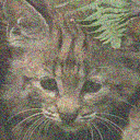
$i=0$	$i=1$	$i=2$	$i=4$	$i=8$
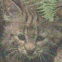
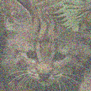
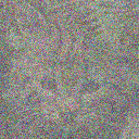
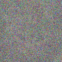
$i=32$	$i=128$	$i=512$	$i=2048$	$i=8192$
(b) osmosis
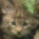
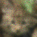
$i=0$	$i=1$	$i=2$	$i=4$	$i=8$
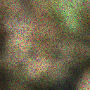
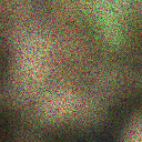
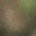
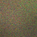
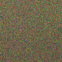
$i=32$	$i=128$	$i=512$	$i=2048$	$i=8192$

Figure 1: The probabilistic diffusion trajectory (a) was obtained with $\beta_{t}=0.02$ and $i$ indicates the number of steps. The osmosis evolution (b) uses time step size $\tau=1$ and a canonical drift vector field of a Gaussian noise image.

4 Probabilistic Diffusion Models and Osmosis

After briefly reviewing osmosis filters, we establish connections to probabilistic diffusion via the PDE formulation, highlighting similarities and differences.

4.1 Continuous Osmosis Filtering

Consider an initial grey value image $f:\Omega\rightarrow\mathbb{R}_{+}$ that maps coordinates from the image domain $\Omega\subset\mathbb{R}^{2}$ to positive grey values. Osmosis describes the evolution of $u:\Omega\times[0,\infty)\rightarrow\mathbb{R}_{+}$ over time $t$, starting with $f$ at $t=0$. Colour images are covered by channel-wise processing. Besides the initial image, the so-called drift vector field $\bm{d}:\Omega\rightarrow\mathbb{R}^{2}$ has a decisive impact on the image evolution of $u(\bm{x},t)$ which is determined by the PDE [30]

$$\partial_{t}u \;=\;\Delta u-\mbox{\rm{\bf{div\,}}}(\bm{d}u) \quad\text{on }\Omega\times(0,T]\,.$$ (26)

Reflecting boundary conditions prevent transport across the image boundaries. For $\bm{d}=\bm{0}$, Eq. (26) describes a homogeneous diffusion process [11], which smoothes the image over time. The drift component $-\mbox{\rm{\bf{div\,}}}(\bm{d}u)=-\partial_{x}(d_{1}u)-\partial_{y}(d_{2}u)$ specifies local asymmetries in exchange of data between pixel cells. This makes it a valuable design tool for filters in visual computing.

The PDE formulation of Feller [5] for probabilistic diffusion from Eq. (24) closely resembles the osmosis equation (26). Consider the 1-D version of the osmosis equation (26):

$$\partial_{t}u \;=\;\partial_{xx}u-\partial_{x}(du) \quad\text{on }\Omega\subset{\mathbb{R}}\times(0,T]\,.$$ (27)

A structural comparison to Eq. (24) reveals that the evolving image $u$ corresponds to the evolving probability density $p$. In both cases, $\partial_{t}$ is the derivative w.r.t. the time variable of the image evolution. The spatial derivative $\partial_{x}$ corresponds to the derivative $\partial_{\bm{u}_{t}}$ w.r.t. positions of individual particles in the probabilistic diffusion model (see Section 4.4). Hence, we can identify $m_{2}$ with a diffusivity which is set to one in the linear osmosis equation. The moment $m_{1}$ corresponds to the scalar drift term $d$ in Eq. (27). Overall, we can interpret probabilistic diffusion as a 1-D osmosis PDE on the probability density $p$. Thus, there is a close conceptual connection between both methods.

In this paper, we consider only those osmosis properties that are most relevant for our comparison to probabilistic diffusion. For the more theoretical details we refer to Weickert et al. [30] in the continuous and Vogel et al. [28] in the discrete setting. Additional theoretical results and their proofs can be found in the Ph.D. thesis of Schmidt [23].

4.2 Visual Comparison

In the following, we compare structural properties of osmosis filtering and probabilistic diffusion models. In order to illustrate our observations, we provide a visual comparison of probabilistic diffusion to an osmosis evolution in Fig. 1. Since the probabilistic diffusion model defines an evolution of probability densities, the visual comparison considers a single, exemplary trajectory. It acts as a representative for the effects on the level of individual images.

Such a trajectory of the probabilistic diffusion model can be directly obtained from the forward process. It is straightforward to implement following the update scheme from Eq. (4), which is already formulated in the discrete setting.

We discretise the continuous osmosis model from Section 4.1 in the same way as Vogel et al. [28]. In particular, we use an implicit scheme with a stabilised BiCGSTAB solver [16]. In order to obtain the osmosis evolution, we use a standard normal noise sample $v$ to define the so-called canonical drift vector field $\bm{d}=\frac{\bm{\nabla}v}{v}$. Weickert et al. [30] have shown that this yields a steady state $w=\frac{\mu_{f}}{\mu_{v}}v$ where $\mu_{u}$ denotes the average grey value of an image $u$.

Note that our visual comparison is not intended as a full-scale, systematic evaluation of both approaches, which is beyond the scale of this paper.

4.3 Common Structural Properties

Due to the observation that both osmosis and probabilistic diffusion rely on drift-diffusion, they share some theoretical properties and yield similar image evolutions in Fig. 1. Starting with the same initial image $f$ from the Berkeley segmentation dataset BSDS500 [2] both processes transition to noise.

We observe that a comparable amount of information of the initial image is removed over time. Schmidt [23] has shown that Lyapunov functionals can be defined for osmosis. In particular, the relative entropy of $u$ w.r.t. $w$,

$$L(t)\;:=\;-\int_{\Omega}u(\bm{x},t)\ln\left(\frac{u(\bm{x},t)}{w(\bm{x})}\right)\,d\bm{x}\,,$$ (28)

is increasing in $t$. It indicates that the information w.r.t. to the steady state is increasing. This conceptually resembles the conditional entropy from Section 3, which is formulated from the point of view of the initial distribution instead.

Finally, the backward process for probabilistic diffusion has a conceptual counterpart in osmosis. By swapping the roles of initial and guidance image, osmosis can also transition from noise to an image. However, this would not yield the same intermediate scales as the osmosis evolution in Fig. 1.

4.4 Differences

In contrast to probabilistic diffusion, osmosis is deterministic and thus has different applications. Osmosis is applied to individual images only, but also does not require any training data to perform tasks like image editing [3, 28, 30] or shadow removal [3, 18, 30]. Due to its stochastic nature, probabilistic diffusion is a natural choice for generating new images from given user prompts such as text. However, it can also be used for the restoration of individual images, e.g. restoring large missing image parts with matching generated content [21, 27].

The second major difference lies in the physical interpretation of images. Osmosis directly models the macroscopic aspects of propagation in the 2-D image domain $\Omega$, where pixel values can be seen as concentrations in the respective area. In contrast, the implementation of probabilistic diffusion via a Markov process models individual particles with 1-D Brownian motion. The pixel values are thus positional data instead, and propagation occurs in the co-domain. Effects of these conceptual differences are visible in Fig. 1. Osmosis gradually reduces the features of the cat by smoothing in the two-dimensional image domain. In contrast, the independent pixel-wise Brownian motion of probabilistic diffusion keeps edges of the original image intact until they are drowned out by noise.

Considering the steady state, we see that osmosis preserves the average colour value of the initial image, while samples from the standard normal distribution in probabilistic diffusion always have zero mean. Note that for osmosis, we only receive a noise steady state since we specified the guidance image accordingly – we can also use arbitrary other images to guide osmosis to receive non-trivial steady states. In contrast, probabilistic diffusion in the sense of Sohl-Dickstein et al. [26] always converges to a tractable (noise) distribution, e.g. the standard normal distribution.

5 Conclusions and Outlook

Investigating probabilistic diffusion from the point of view of scale-space research yields surprising results: Probabilistic diffusion defines an evolution that resembles traditional scale-spaces in important aspects such as causality and gradual simplification. However, probabilistic diffusion acts on distributions rather than on individual images and removes information by creating chaos instead of uniformity. Thus, it does not converge to a flat steady state, but to a noise distribution. Theoretical and practical results allow bi-directional traversal of this scale-space, which is rare in deterministic scale-spaces.

Interestingly, probabilistic diffusion can be seen as the stochastic counterpart to classical PDE-based, deterministic osmosis filtering. In the future, we plan to investigate this connection in more detail. Moreover, recognising probabilistic diffusion as a scale-space implies potential applications that make use of intermediate results of the evolution instead of only relying on steady states.

Acknowledgements: I thank Joachim Weickert, Karl Schrader, and Kristina Schaefer for fruitful discussions and advice.

References

- [1] Alvarez, L., Guichard, F., Lions, P.L., Morel, J.M.: Axioms and fundamental equations in image processing. Archive for Rational Mechanics and Analysis 123, 199–257 (Sep 1993)
- [2] Arbelaez, P., Maire, M., Fowlkes, C., Malik, J.: Contour detection and hierarchical image segmentation. IEEE Transactions on Pattern Analysis and Machine Intelligence 33(5), 898–916 (Aug 2011)
- [3] d’Autume, M., Morel, J.M., Meinhardt-Llopis, E.: A flexible solution to the osmosis equation for seamless cloning and shadow removal. In: Proc 2018 IEEE International Conference on Image Processing. pp. 2147–2151. Athens, Greece (Oct 2018)
- [4] Duits, R., Florack, L., de Graaf, J., ter Haar Romeny, B.: On the axioms of scale space theory. Journal of Mathematical Imaging and Vision 20, 267–298 (May 2004)
- [5] Feller, W.: On the theory of stochastic processes, with particular reference to applications. In: First Berkeley Symposium on Mathematical Statistics and Probability. pp. 403–432. Berkeley, CA (Jan 1949)
- [6] Gardiner, C.W.: Handbook of Stochastic Methods for Physics, Chemistry and the Natural Sciences, Springer Series in Synergetics, vol. 13. Springer, Berlin (1985)
- [7] Goodfellow, I.J., Pouget-Abadie, J., Mirza, M., Xu, B., Warde-Farley, D., Ozair, S., Courville, A.C., Bengio, Y.: Generative adversarial nets. In: Ghahramani, Z., Welling, M., Cortes, C., Lawrence, N.D., Weinberger, K.Q. (eds.) Proc. 28th International Conference on Neural Information Processing Systems. Advances in Neural Information Processing Systems, vol. 27, pp. 2672–2680. Montréal, Canada (Dec 2014)
- [8] Hagemann, P.L., Hertrich, J., Steidl, G.: Generalized normalizing flows via Markov chains. In: Elements in Non-local Data Interactions: Foundations and Applications. Cambridge University Press (2023), in press
- [9] Ho, J., Jain, A., Abbeel, P.: Denoising diffusion probabilistic models. In: Advances in Neural Information Processing Systems, vol. 33, pp. 6840–6851. NeurIPS Foundation, San Diego, CA (2020)
- [10] Huckemann, S., Kim, K.R., Munk, A., Rehfeldt, F., Sommerfeld, M., Weickert, J., Wollnik, C.: The circular sizer, inferred persistence of shape parameters and application to early stem cell differentiation. Bernoulli 22(4), 2113–2142 (Nov 2016)
- [11] Iijima, T.: Basic theory on normalization of pattern (in case of typical one-dimensional pattern). Bulletin of the Electrotechnical Laboratory 26, 368–388 (Jan 1962), in Japanese
- [12] Kingma, D., Salimans, T., Poole, B., Ho, J.: Variational diffusion models. Advances in neural information processing systems 34, 21696–21707 (2021)
- [13] Koenderink, J.J., Van Doorn, A.J.: The structure of locally orderless images. International Journal of Computer Vision 31(2), 159–168 (Apr 1999)
- [14] Lindeberg, T.: Generalized Gaussian scale-space axiomatics comprising linear scale-space, affine scale-space and spatio-temporal scale-space. Journal of Mathematical Imaging and Vision 40, 36–81 (2011)
- [15] Majer, P.: A statistical approach to feature detection and scale selection in images. Ph.D. thesis, Department of Mathematics, Saarland University, Göttingen, Germany (2000)
- [16] Meister, A.: Numerik linearer Gleichungssysteme. Vieweg, Braunschweig, 5th edn. (2015)
- [17] Parisotto, S., Calatroni, L., Bugeau, A., Papadakis, N., Schönlieb, C.B.: Variational osmosis for non-linear image fusion. IEEE Transactions on Image Processing 29, 5507–5516 (Apr 2020)
- [18] Parisotto, S., Calatroni, L., Caliari, M., , Schönlieb, C.B., Weickert, J.: Anisotropic osmosis filtering for shadow removal in images. Inverse Problems 35(5) (Apr 2019), article 054001
- [19] Pedersen, K.S.: Properties of Brownian image models in scale-space. In: Griffin, L.D., Lillholm, M. (eds.) Scale-Space Methods in Computer Vision, Lecture Notes in Computer Science, vol. 2695, pp. 281–296. Springer, Berlin (2003)
- [20] Risken, H.: The Fokker–Planck Equation. Springer, New York (1984)
- [21] Rombach, R., Blattmann, A., Lorenz, D., Esser, P., Ommer, B.: High-resolution image synthesis with latent diffusion models. In: Proc. 2022 IEEE/CVF Conference on Computer Vision and Pattern Recognition. pp. 10684–10695. New Orleans, LA (Jun 2022)
- [22] Scherzer, O., Weickert, J.: Relations between regularization and diffusion filtering. Journal of Mathematical Imaging and Vision 12(1), 43–63 (Feb 2000)
- [23] Schmidt, M.: Linear Scale-Spaces in Image Processing: Drift–Diffusion and Connections to Mathematical Morphology. Ph.D. thesis, Department of Mathematics, Saarland University, Saarbrücken, Germany (2018)
- [24] Schmidt, M., Weickert, J.: Morphological counterparts of linear shift-invariant scale-spaces. Journal of Mathematical Imaging and Vision 56(2), 352–366 (Oct 2016)
- [25] Sochen, N.A.: Stochastic processes in vision: From Langevin to Beltrami. In: Proc. Eighth International Conference on Computer Vision. vol. 1, pp. 288–293. Vancouver, Canada (Jul 2001)
- [26] Sohl-Dickstein, J., Weiss, E., Maheswaranathan, N., Ganguli, S.: Deep unsupervised learning using nonequilibrium thermodynamics. In: Bach, F., Blei, D. (eds.) Proc. 32nd International Conference on Machine Learning. Proceedings of Machine Learning Research, vol. 37, pp. 2256–2265. Lille, France (Jul 2015)
- [27] Song, Y., Durkan, C., Murray, I., Ermon, S.: Maximum likelihood training of score-based diffusion models. Advances in Neural Information Processing Systems 34, 1415–1428 (2021)
- [28] Vogel, O., Hagenburg, K., Weickert, J., Setzer, S.: A fully discrete theory for linear osmosis filtering. In: Kuijper, A., Bredies, K., Pock, T., Bischof, H. (eds.) Scale Space and Variational Methods in Computer Vision, Lecture Notes in Computer Science, vol. 7893, pp. 368–379. Springer, Berlin (2013)
- [29] Weickert, J.: Anisotropic Diffusion in Image Processing. Teubner, Stuttgart (1998)
- [30] Weickert, J., Hagenburg, K., Breuß, M., Vogel, O.: Linear osmosis models for visual computing. In: Heyden, A., Kahl, F., Olsson, C., Oskarsson, M., Tai, X.C. (eds.) Energy Minimisation Methods in Computer Vision and Pattern Recognition, Lecture Notes in Computer Science, vol. 8081, pp. 26–39. Springer, Berlin (2013)