Maximum quantum battery charging power is not an entanglement monotone

Beneficial and detrimental entanglement for quantum battery charging

Abstract

We establish a general implementation-independent approach to assess the potential advantage of using highly entangled quantum states between the initial and final states of the charging protocol to enhance the maximum charging power of quantum batteries. It is shown that the impact of entanglement on power can be separated from both the global quantum speed limit associated to an optimal choice of driving Hamiltonian and the energy gap of the batteries. We then demonstrate that the quantum state advantage of battery charging, defined as the power obtainable for given quantum speed limit and battery energy gap, is not an entanglement monotone. A striking example we provide is that, counterintuitively, independent thermalization of the local batteries, completely destroying any entanglement, can lead to larger charging power than that of the initial maximally entangled state. Highly entangled states can thus also be potentially disadvantageous when compared to product states. We also demonstrate that taking the considerable effort of producing highly entangled states, such as W or $k$-locally entangled states, is not sufficient to obtain quantum-enhanced scaling behavior with the number of battery cells. Finally, we perform an explicit computation for a Sachdev-Ye-Kitaev battery charger to demonstrate that the quantum state advantage allows the instantaneous power to exceed its classical bound.

I Introduction

The modern notion of a “quantum advantage” has its origin in the potential of quantum computers to outperform their classical counterparts et al. (2020); Madsen et al. (2022). Other areas of information technology, for which a quantum advantage can be defined, are for example metrology Giovannetti et al. (2004); Braun et al. (2018) which has inter alia been used in gravitational wave astronomy Collaboration (2011), or cryptography Gisin et al. (2002) and communication Gisin and Thew (2007).

Where however quantum advantage seems to be most relevant for many practical reasons is on the field of energy storage and retrieval Auffèves (2022). Quantum battery research has focused on concrete means to increase charging power Binder et al. (2015); Campaioli et al. (2017, 2018); Carrasco et al. (2022); Rossini et al. (2020); Gyhm et al. (2022) as well as on work extraction Alicki and Fannes (2013); Hovhannisyan et al. (2013); García-Pintos et al. (2020); Barra (2019); Shi et al. (2022); Šafránek et al. (2023), see for a review including quantum thermodynamical aspects Bhattacharjee and Dutta (2021). In addition to these theoretical studies, increasingly progress has very recently been made towards an experimental realization of quantum batteries et al. (2022a, b); Joshi and Mahesh (2022); Cruz et al. (2022).

Quantum technology is generally driven by the increasing demand for a practically useful quantum advantage, which however can be an ambiguous and strongly model dependent notion Andolina et al. (2019). One may conjecture that entanglement is the most important resource for the quantum advantage of charging, see, e.g., Refs. Ferraro et al. (2018); Julià-Farré et al. (2020), but results to the contrary have been found Kamin et al. (2020); Le et al. (2018). As far as we are aware, there is however no general device- and implementation-independent relation which expresses the potential advantage of using entangled states solely in terms of an arbitrary quantum state specified by the density matrix operator ${\hat{\rho}}$. Our major aim in this work is to fill this gap, such as to be able to quantify in a general manner how entanglement contributes to quantum advantage.

Physical mechanisms affecting the maximal charging power are the external driving for the charging, the general battery setup, and the energy gap between the ground state and the excited state of the batteries Julià-Farré et al. (2020); Campaioli et al. (2018). We show in the following that the maximum charging power can be classified and separated into three parts, the energy gap of the batteries, the quantum speed limit associated to the time dependent driving Hamiltonian, and what one may call a genuine quantum state advantage depending solely on the quantum state. We thereby provide a general relation rigorously establishing the relation of entanglement and quantum charging advantage, by isolating the impact of entanglement from the quantum speed limit and the energy gap. We note in this regard that the energy gap and quantum speed limit constitute “trivial” advantages in the sense that one is always able to obtain a higher charging power from the faster time evolution of the quantum state and from a large energy gap. Isolating these, we aim at finding the optimal charging path in the Hilbert space outperforming the classical parallel charging protocol. This can then represent a genuine quantum state advantage of charging, because this Hilbert space trajectory is determined by whether the states are entangled or not. We point out in this regard, and importantly for our argument, that the quantum speed limit (QSL) has no bias to be enhanced by entanglement in a given quantum state. Specifically, the QSL samples the full Hilbert space generated by arbitrarily choosing the driving Hamiltonians. It can therefore not depend on any kind of bi- or multi-partition of the system, and thus also not on any corresponding measure of entanglement.

By isolating the quantum advantage related to entanglement, we obtain an explicit expression for the entanglement contribution to charging power, from which it generally follows that while entanglement is necessary for a quantum state advantage over classical charging, it is not sufficient, cf. Ref. Campaioli et al. (2018). We thus establish the latter fact in a device- and implementation-independent way. We find that certain varieties of entanglement can diminish charging power and prove, as a theorem, that quantum state advantage is not an entanglement monotone. We demonstrate this for a number of examples. Therefore, the quantum advantage of battery charging cannot constitute a measure of entanglement.

After introducing the general battery setup, we discuss the conventional approach for evaluating the power bound via the covariance matrix, which is however, as we show, hampered by containing also classical in addition to quantum correlations. To resolve this, we introduce what we coin a commutation matrix, and from this establish the fundamental entanglement-determined bound on charging power. Our approach explicitly demonstrates that it is not possible to assess the maximally possible quantum advantage of battery charging solely with an entanglement measure. This leads, inter alia, to the (at first glance counterintuitive) possibility that increasing charging power can potentially be achieved by destroying entanglement, e.g., by thermalization. We show this explicitly for highly entangled initial states during their Lindbladian evolution to thermalized states. We also demonstrate, for globally entangled W and $k$-locally entangled pure states, that their quantum state advantage does not display a scaling with the number of cells $N$. Therefore, their obtainable power does not scale faster than linear in $N$. We perform furthermore an explicit computation for Sachdev-Ye-Kitaev batteries Rossini et al. (2020) demonstrating that the quantum state advantage defined by us indeed peaks at approximately the same time as the instantaneous power does.

We provide our major results in the main text, and defer detailed derivations and proofs to an Appendix.

II Quantum battery power

We consider a quantum battery setup composed of independent cells, with Hamiltonian $\hat{H}=\sum_{i=1}^{N}\hat{H}_{i}\bigotimes_{j\neq i}\hat{I}_{j}$, where $\hat{H}_{i}$ indicates the Hamiltonian of the $i$th cell. At time $t$ an instantaneous quantum state of the battery, represented by a density matrix ${\hat{\rho}}(t)$, evolves due to switching on for a finite time a time-dependent driving Hamiltonian, $\hat{V}(t)$ (which contains the time independent battery part $\hat{H}$), according to the von Neumann equation ($\hbar=1$)

$$\frac{\partial{\hat{\rho}}}{\partial t}=i[{\hat{\rho}},\hat{V}(t)].$$ (1)

The energy stored in the battery is $E(t)=\mathrm{tr}(\hat{H}{\hat{\rho}})$ and the instantaneous battery charging power is then defined as a change in the (expectation value of the) energy stored in the battery cells per unit of time,

$$P(t)=\mathrm{tr}\left(\hat{H}\,\frac{\partial{\hat{\rho}}}{\partial t}\right)=\mathrm{tr}\left(i\hat{H}[{\hat{\rho}},\hat{V}(t)]\right).$$ (2)

We aim at determining to which extent the entanglement of the state ${\hat{\rho}}$ impacts the upper bound on the power of battery charging. This can be reformulated as determining the maximum instantaneous power of battery charging we can obtain from the state ${\hat{\rho}}(t)$ by manipulating $\hat{V}(t)$.

The relation $P=\mathrm{tr}\left(i\hat{H}[{\hat{\rho}},\hat{V}(t)]\right)=\mathrm{tr}\left(i[\hat{H},\hat{V}(t)]{\hat{\rho}}\right)$ for the instantaneous power, defining variances of operators by $\langle\Delta\bm{\cdot}^{2}\rangle=\mathrm{tr}(\bm{\cdot}^{2}{\hat{\rho}})-\mathrm{tr}(\bm{\cdot}{\hat{\rho}})^{2}$, then reads by the Heisenberg-Robertson inequality

$$P(t)\leq 2\sqrt{\langle\Delta\hat{V}^{2}(t)\rangle\langle\Delta\hat{H}^{2}\rangle}.$$ (3)

This implies that the standard deviations of $\hat{V}(t)$ and $\hat{H}$ determine the bound of power Julià-Farré et al. (2020), and leads one to conjecture that the covariance matrix  Gühne et al. (2007); Li et al. (2008); Gittsovich and Gühne (2010), which generally relates to the variance of any given set of observables, can be applied to assess the quantum state advantage of battery charging.

III Covariance matrix approach

III.1 Definition of covariance matrix

We briefly review the definition of the covariance matrix of multipartite systems and its properties. Covariance matrices, familiar from continuous variable systems (in particular for Gaussian states), were introduced by Refs. Gühne et al. (2007); Li et al. (2008); Gittsovich and Gühne (2010), to address the separability of finite-dimensional quantum states, and were demonstrated to provide a reasonably general framework to capture entanglement, in particular also by linking the covariance matrix criterion to previously established criteria for entanglement.

To be able to define the covariance matrix, we need to first establish a set of local observables. We assume the $i$th cell lives in an $n_{i}$-dimensional Hilbert space. The local observable set of the $i$th cell, $\hat{\bm{M}^{i}}$, has $n_{i}^{2}$ elements

$$\hat{\bm{M}^{i}}=\{\bigotimes_{j\neq i}\hat{I}^{j}\otimes A^{i}_{1},\cdots,\bigotimes_{j\neq i}\hat{I}^{j}\otimes A^{i}_{n_{i}^{2}}\},$$ (4)

where the $A_{\alpha}^{i}$ constitute the members of the Lie algebra of $U(n_{i})$. Importantly, we impose the following Lie algebra orthonormality condition Gühne et al. (2007),

$${\mathrm{tr}(\hat{A^{i}_{\alpha}}\hat{A^{i}_{\beta}})=\delta_{\alpha\beta}\,\quad\forall\,i}$$ (5)

on the operators contained in the set of observables, where the $\alpha,\beta$ indices run over $1,\ldots,n_{i}^{2}$. The orthonormality condition is imposed to be able to render the norm of the covariance matrices in Eq. (7) below independent of the observables set $\hat{\bm{M}}$, then leaving only state dependence of the operator norm.

The total set of observables is the union of the local cell observables as follows

$$\hat{\bm{M}}=\bigcup_{i=1}^{N}\hat{\bm{M}^{i}}=\{\hat{M}_{\mu}\}$$ (6)

The covariance matrix $\gamma({\hat{\rho}},\hat{\bm{M}})$ is then defined as the symmetrized correlation function,

$$\gamma({\hat{\rho}},\hat{\bm{M}})_{\mu\nu}=\tfrac{1}{2}\langle\hat{M_{\mu}}\hat{M_{\nu}}+\hat{M_{\nu}}\hat{M_{\mu}}\rangle-\langle\hat{M_{\mu}}\rangle\langle\hat{M_{\nu}}\rangle,$$ (7)

which is a symmetric, real, and positive semidefinite matrix.  Here, indices $\mu,\nu$ run over both $i$ and $\alpha$ indices.

We make use of the following properties of the covariance matrix $\gamma$. First, the eigenvalues of $\gamma({\hat{\rho}},\hat{\bm{M}})$ are independent of the observable set $\hat{\bm{M}}$ when the orthonormality condition (5) is met. Another property is that the variance of $\hat{H}$ obeys an inequality involving $\gamma$. To establish that inequality, we use that the Hamiltonian can be written as a linear decomposition using the operator set $\hat{\bm{M}}$ Gühne et al. (2007). Employing a normalized real vector, ${\bm{u}}$, $\hat{H}=\hat{\bm{M}}\cdot{\bm{u}}\sqrt{\sum_{i=1}^{N}\mathrm{tr}(\hat{H}_{i}^{2})}$, we have

$$\begin{split}\langle\Delta\hat{H}^{2}\rangle&={\bm{u}}^{\mathrm{T}}\gamma({\hat{\rho}},\hat{\bm{M}}){\bm{u}}\sum_{i=1}^{N}\mathrm{tr}(\hat{H}_{i}^{2})\\ &\leq\|\gamma({\hat{\rho}},\hat{\bm{M}})\|\sum_{i=1}^{N}\mathrm{tr}(\hat{H}_{i}^{2}),\end{split}$$ (8)

from which we can infer the bound on the charging power by using (3),

$$P\leq 2\sqrt{\|\gamma({\hat{\rho}},\hat{\bm{M}})\|\sum_{i=1}^{N}\mathrm{tr}(\hat{H}_{i}^{2})\langle\Delta\hat{V}^{2}\rangle},$$ (9)

where the operator norm $\|\bm{\cdot}\|$ of a Hermitian operator is its largest eigenvalue Hassani (2013). In addition, $\|\gamma({\hat{\rho}},\hat{\bm{M}})\|$ is bounded by $\frac{N}{2}$ and is equal to $\frac{1}{2}$ for a product state, $|\psi\rangle=\bigotimes_{i=1}^{N}|\psi_{i}\rangle$. Finally, $\|\gamma({\hat{\rho}},\hat{\bm{M}})\|$ is conserved by local unitary evolution Julià-Farré et al. (2020).

III.2 Issues with the covariance matrix approach

From the fact that $\|\gamma({\hat{\rho}},\hat{\bm{M}})\|$ is invariant for any pure product state, one tends to infer that $\|\gamma({\hat{\rho}},\hat{\bm{M}})\|$ represents a suitable measure to assess to which extent entanglement contributes to the power bound. Indeed entanglement contributes for a pure state, but however not generally when one is dealing with a mixed state.

In particular, mixed states can increase $\|\gamma({\hat{\rho}},\hat{\bm{M}})\|$ although they do not enlarge the bound on power. To illustrate this with a concrete example, the mixed state ${\hat{\rho}}=(|00\rangle\langle 00|+|11\rangle\langle 11|)/2$ has $\|\gamma({\hat{\rho}},\hat{\bm{M}})\|=1$ larger than $\frac{1}{2}$ for simple product states. This mixed state thus seems to indicate a factor two advantage over product states. However, this is not the case, which can be seen as follows.

By decomposing ${\hat{\rho}}$ into the normalized sum of ${\hat{\rho}}_{1}=|00\rangle\langle 00|$ and ${\hat{\rho}}_{2}=|11\rangle\langle 11|$, we rewrite Eq. (3) as

$$P\leq\frac{1}{2}(\mathrm{tr}([-i[\hat{H},\hat{V}],{\hat{\rho}}_{1}])+\mathrm{tr}([-i[\hat{H},\hat{V}],{\hat{\rho}}_{2}])).$$ (10)

This yields, using (9),

$$P\leq\sum_{l=1,2}\sqrt{\|\gamma({\hat{\rho}}_{l},\hat{\bm{M}})\|\sum_{i=1}^{N}\mathrm{tr}(\hat{H}_{i}^{2})\langle\Delta\hat{V}^{2}\rangle_{l}},$$ (11)

where $\langle\Delta\hat{V}^{2}\rangle_{l}=\mathrm{tr}(\hat{V}^{2}{\hat{\rho}}_{l})-\mathrm{tr}(\hat{V}{\hat{\rho}})^{2}$. Since

$$\frac{1}{2}\left(\sqrt{\langle\Delta\hat{V}^{2}\rangle_{1}}+\sqrt{\langle\Delta\hat{V}^{2}\rangle_{2}}\right)\leq\sqrt{\langle\Delta\hat{V}^{2}\rangle}$$ (12)

and both $\|\gamma({\hat{\rho}}_{l},\hat{\bm{M}})\|$ are equal to $\frac{1}{2}$, we obtain finally that

$$P\leq\sqrt{2\sum_{i=1}^{N}\mathrm{tr}(\hat{H}_{i}^{2})\mathrm{tr}(\Delta\hat{V}^{2})},$$ (13)

identical to the product state bound, thus leading to a tighter bound than that in (9) when one sets $\|\gamma({\hat{\rho}},\hat{\bm{M}})\|=1$ for the non-decomposed mixed state therein. This provides evidence that the covariance matrix $\gamma$ also contains classical correlations.

We show below that, generally, there is no quantum state advantage from separable states over product states. Mixed states can increase $\|\gamma({\hat{\rho}},\hat{\bm{M}})\|$, however inequality (9) is thereby rendered a loose bound and the inequality on the power cannot be saturated.

In summary, the inequality (9) only furnishes a loose, non-saturable bound on the charging power, in which, in particular, the impact of a quantum speed limit (which does not give a directly entanglement-related factor in the power bound) is not manifest. To address these issues, let us define the what we coin the commutation matrix.

IV commutation matrix

IV.1 Definition

To eliminate the above discussed impact of classical correlations, we define the commutation matrix $\gamma_{C}({\hat{\rho}},\hat{\bm{M}})$ as follows

$$\gamma_{C}({\hat{\rho}},\hat{\bm{M}})_{\mu\nu}\coloneqq-\mathrm{tr}([\hat{M_{\mu}},\sqrt{{\hat{\rho}}}][\hat{M_{\nu}},\sqrt{{\hat{\rho}}}]),$$ (14)

for the same orthonormalized observable set $\hat{\bm{M}}$ displayed in Eq. (6), used already for the covariance matrix. Since ${\hat{\rho}}$ is positive semidefinite, $\sqrt{{\hat{\rho}}}$ is well-defined as a positive semidefinite matrix. The matrix $\gamma_{C}({\hat{\rho}},\hat{\bm{M}})$ has similar properties as $\gamma({\hat{\rho}},\hat{\bm{M}})$: Also $\gamma_{C}({\hat{\rho}},\hat{\bm{M}})$ is positive semidefinite and its eigenvalues only depend on the quantum state for all observables in the set which meet the orthonormality condition (5). We derive these and other properties of the commutation matrix in Appendix A.

IV.2 Power bound

Crucial for our argument in the following is the property that $\|\gamma_{C}({\hat{\rho}},\hat{\bm{M}})\|$ is only a function of the quantum state encoded in the density matrix, ${\hat{\rho}}$. We denote this function as

$$\Gamma_{C}({\hat{\rho}})\coloneqq\|\gamma_{C}({\hat{\rho}},\hat{\bm{M}})\|.$$ (15)

Using this definition of $\Gamma_{C}({\hat{\rho}})$ in terms of our commutation matrix, we now obtain a tighter bound than Eq. (9):

Theorem 1.

The instantaneous power of the quantum battery is bounded as follows

$$P\leq\sqrt{2\kappa\Gamma_{C}({\hat{\rho}})\sum_{i=1}^{N}\mathrm{tr}(\hat{H}_{i}^{2})\langle\Delta\hat{V}^{2}\rangle},$$ (16)

where the coefficient $\kappa$ lies within the range $1\leq\kappa\leq 2$ (see Appendix B), and we neglect a possible weak dependence of $\kappa$ on ${\hat{\rho}}$ and $\hat{V}$ for mixed states; for any pure state, $\kappa=1$. Equality and thus saturation of the bound (16) is met when the two conditions

$$\{\sqrt{{\hat{\rho}}},\hat{V}\}=i[\hat{H},\sqrt{{\hat{\rho}}}]\sqrt{-\frac{\mathrm{tr}(\{\sqrt{{\hat{\rho}}},\hat{V}\}^{2})}{\mathrm{tr}([\hat{H},\sqrt{{\hat{\rho}}}]^{2})}}$$ (17)

$$\hat{H}=\hat{\bm{M}}\cdot{\bm{u}}\sqrt{\sum_{i=1}^{N}\mathrm{tr}(\hat{H}_{i}^{2})}$$ (18)

are fulfilled. Here, ${\bm{u}}$ is the normalized eigenvector of $\gamma_{C}({\hat{\rho}},\hat{\bm{M}})$ which has the eigenvalue $\Gamma_{C}({\hat{\rho}})$. The theorem on the power bound can be proved as follows.

Proof.

By the Cauchy-Schwarz inequality, we have

$$P(t)=\mathrm{tr}(i[\hat{H},\sqrt{{\hat{\rho}}}]\{\sqrt{{\hat{\rho}}},\hat{V}\})\\ \leq\sqrt{-\mathrm{tr}([\hat{H},\sqrt{{\hat{\rho}}}]^{2})\mathrm{tr}(\{\sqrt{{\hat{\rho}}},\hat{V}\}^{2})}$$ (19)

from which the first equality condition (17) derives. Moreover, we can always choose a $\hat{V}$ which satisfies (17). A detailed method to choose an optimal $\hat{V}$ is provided by Eq. (54) in Appendix B.

We now establish how $2\kappa\langle\Delta\hat{V}^{2}\rangle$ derives from $\mathrm{tr}(\{\sqrt{{\hat{\rho}}},\hat{V}\}^{2})$. First of all, we obtain, by using the fact that $\Gamma_{C}$ is the largest eigenvalue of $\gamma_{C}({\hat{\rho}},\hat{\bm{M}})$ [cf. Eq. (49)]

$$-\mathrm{tr}([\hat{H},\sqrt{{\hat{\rho}}}]^{2})\leq\Gamma_{C}({\hat{\rho}})\sum_{i=1}^{N}\mathrm{tr}(\hat{H}_{i}^{2}).$$ (20)

Since adding real multiples of the identity operator to $\hat{V}$ does not contribute to the power, the bound on the power in Eq. (19) can be rewritten as follows (with real $\lambda$):

$$P\leq\min_{\lambda}\sqrt{\Gamma_{C}({\hat{\rho}})\sum_{i=1}^{N}\mathrm{tr}(\hat{H}_{i}^{2})\mathrm{tr}(\{\sqrt{{\hat{\rho}}},\hat{V}+\lambda\hat{I}\}^{2})}$$ (21)

The term $\mathrm{tr}(\{\sqrt{{\hat{\rho}}},\hat{V}+\lambda\hat{I}\}^{2})$ on the right-hand side of (21) is minimized by $2\mathrm{tr}({\hat{\rho}}\hat{V}^{2})+2\mathrm{tr}(\sqrt{{\hat{\rho}}}\hat{V}\sqrt{{\hat{\rho}}}\hat{V})-4\mathrm{tr}({\hat{\rho}}\hat{V})^{2}$ when $\lambda$ is equal to $-\mathrm{tr}(\hat{V}{\hat{\rho}})$. By the inequality $\mathrm{tr}({\hat{\rho}}\hat{V})^{2}\leq\mathrm{tr}(\sqrt{{\hat{\rho}}}\hat{V}\sqrt{{\hat{\rho}}}\hat{V})\leq\mathrm{tr}({\hat{\rho}}\hat{V}^{2})$, we can replace $\mathrm{tr}(\{\sqrt{{\hat{\rho}}},\hat{V}\}^{2})$ by $2\kappa\langle\Delta\hat{V}^{2}\rangle$, for $1\leq\kappa\leq 2$. The latter inequality is derived by using that $-\mathrm{tr}([\hat{V},\sqrt{{\hat{\rho}}}]^{2})\geq 0$ and $\mathrm{tr}(\hat{V}\sqrt{{\hat{\rho}}}\hat{V}\sqrt{{\hat{\rho}}})\geq 0$. This completes the proof of the inequality (16); we provide further details in Appendix B. ∎

V Properties of derived power bound

V.1 Isolating the impact of quantum speed limit

To compare driving Hamiltonians composed, e.g., only of local or global battery operations (or a combination of these), and their impact on the power bound, we first explain the form of the QSL constraint we impose. It directly derives from the time-energy uncertainty relation Deffner and Campbell (2017). The standard deviation of the driving Hamiltonian, for all possible drivings $\hat{V}$, yields an effective driving gap $\Delta E$. The latter is given by the time average of the standard deviation of the charging operator as follows (called the constraint $C_{1}$ in Ref. Campaioli et al. (2017))

$$\Delta E=\int_{0}^{T}\frac{\sqrt{\langle\Delta\hat{V}^{2}\rangle}}{T}dt=\Delta E_{\mathrm{single}}\times\sqrt{N},$$ (22)

where we assume that the single-cell gap $\Delta E_{\mathrm{single}}$ does not depend on $\hat{V}$. The above relation restricts the mean of the speed of time evolution of states in Hilbert space by imposing a finite gap $\Delta E$.

We impose in the following the stronger constraint

$$\sqrt{\langle\Delta\hat{V}^{2}\rangle}=\mathrm{constant}\times\sqrt{N},$$ (23)

which restricts the instantaneous rather than just the global speed of time evolution as specified by (22). The constant contained here equals $\Delta E_{\mathrm{single}}$contained in (22) when the condition (23) is imposed.

Note the constraint (23) restricts the evolution speed of states in the Hilbert space independent from entanglement, due to the fact that the choice of the driving Hamiltonian is free and the quantum state resides in the full corresponding Hilbert space when determining the QSL. That is, any kind of bi- or multi-partition of the given state is not allowed to affect the QSL. Therefore, and importantly for our present argument, isolating the QSL in the inequality for the power does not impact assessing the influence of entanglement contained in the state ${\hat{\rho}}$ on the maximum power obtainable.

V.2 Scaling with cell number

Under the condition (23), both $\sum_{i=1}^{N}\mathrm{tr}(\hat{H}_{i}^{2})$ and $\langle\Delta\hat{V}^{2}\rangle$ have linear scaling with $N$, so that $\sqrt{\sum_{i=1}^{N}\mathrm{tr}(\hat{H}_{i}^{2})\langle\Delta\hat{V}^{2}\rangle}$ also has linear scaling with $N$, which is equivalent to classical scaling for the power without quantum state advantage.

When the energy gap and quantum speed limit are given, $\Gamma_{C}({\hat{\rho}})$ therefore indicates a true quantum advantage, related to a geometric advantage in the Hilbert space related to entanglement, which is, in particular, isolated from the QSL.

Entanglement is in fact necessary (but not sufficient, also see below) to exceed the classical linear scaling of the power in the number of cells $N$. One can see this as follows. As the quantum state advantage can be calculated by $\Gamma_{C}({\hat{\rho}})$, we can anticipate the maximum power of a quantum battery. To that end, we use that $\sqrt{\Gamma_{C}({\hat{\rho}})}$ is bounded by $\sqrt{N}$ (Proposition 2 in Appendix A), and is less than or equal to unity for separable states which by definition do not have entanglement. This indicates that the maximum quantum state advantage is $\sqrt{N}$ and there is no quantum advantage without entanglement. This is in agreement with the result for the maximum quantum advantage obtained by Campaioli et al. (2017). We can thus indeed quantify the genuine quantum state advantage for all states by $\sqrt{\Gamma_{C}({\hat{\rho}})}$.

V.3 Achievability of bound

The upper bound contained in (16) is achievable for all kinds of states by manipulating $\hat{H}$ and $\hat{V}$. On the other hand, the power bound can not be saturated for given $\hat{V}$ and $\hat{H}$. One of the factors leading to a nonsaturated bound is a deviation of $\hat{V}$ from the optimal driving Hamiltonian: Imposing a restriction on $\hat{V}$ leads to a reduced power bound, which can be quantified by

$$\cos{\theta_{\hat{V}}}=-\frac{\mathrm{tr}([i[\hat{H},\sqrt{{\hat{\rho}}}]\{\sqrt{{\hat{\rho}}},\hat{V}\})^{2}}{\mathrm{tr}([\hat{H},\sqrt{{\hat{\rho}}}]^{2})\mathrm{tr}(\{\sqrt{{\hat{\rho}}},\hat{V}\}^{2})}.$$ (24)

The structure of $\hat{H}$ also affects the power bound, since commonly $\hat{H}$ is assumed to be fixed and not controllable, in distinction to the driving Hamiltonian $\hat{V}$. This effect is expressed by another angle

$$\cos{\theta_{\hat{H}}}=\frac{-\mathrm{tr}([\hat{H},\sqrt{{\hat{\rho}}}]^{2})}{\Gamma_{C}({\hat{\rho}})\sum_{i=1}^{N}\mathrm{tr}(\hat{H}_{i}^{2})}.$$ (25)

The two angles defined as in the above yield an equation for the power, cf. Appendix. C,

$$P=\sqrt{2\kappa\Gamma_{C}({\hat{\rho}})\sum_{i=1}^{N}\mathrm{tr}(\hat{H}_{i}^{2})\langle\Delta\hat{V}^{2}\rangle\cos{\theta_{\hat{V}}}\cos{\theta_{\hat{H}}}}.$$ (26)

From this expression, we note that the driving Hamiltonian $\hat{V}$ should increase $\Gamma_{C}$ during time evolution. Driving Hamiltonians constructed from simple sums of local operators can however not increase entanglement, as dictated by the condition that every conceivable entanglement measure should not increase by local operations and classical communication (LOCC) Nielsen (1999); Bennett et al. (1999); Vidal (2000). This suggests that states evolved by such driving Hamiltonians starting from the ground state can not have $\Gamma_{C}$ exceeding unity: There is by definition no quantum state advantage from sums of local driving Hamiltonians.

VI Examples for quantum state advantage and disadvantage

We study below in detail the properties of $\Gamma_{C}$ for several examples. We will find that $\Gamma_{C}$ is not an entanglement monotone. This fact can lead to a counterintuitive behavior of the (supposedly) quantum origin of charging power.

To quantify the entanglement in a given state ${\hat{\rho}}$, we employ the negativity, demonstrated to yield an entanglement monotone by Vidal and Werner (2002). For a bipartite system composed, say, of partitions $A$ and $B$, the definition of negativity, ${\mathcal{N}}({\hat{\rho}})$, employs ${\hat{\rho}}^{\mathrm{T_{A}}}$, the partial transpose operation on an $A$-dimensional part of the full density matrix ${\hat{\rho}}$,

$${\mathcal{N}}=\frac{\|{\hat{\rho}}^{\mathrm{T_{A}}}\|_{\mathrm{Tr}}-1}{2}.$$ (27)

Here, $\|{\hat{\rho}}^{\mathrm{T_{A}}}\|_{\mathrm{Tr}}$ is the trace norm, which is the sum of the absolute values of the eigenvalues of ${\hat{\rho}}^{\mathrm{T_{A}}}$.

VI.1 Initial GHZ state and thermalization

We first argue that generally the quantum state advantage $\Gamma_{C}({\hat{\rho}})$ satisfies the following

Theorem 2.

$\Gamma_{C}$ is not an entanglement monotone.

Proof.

We prove the theorem by a counterexample. In particular, LOCC operations can lead to an increase of $\Gamma_{C}$. Suppose the initial state is prepared to be $|\psi_{i}\rangle=\frac{1}{\sqrt{3}}(|00\rangle+|11\rangle+|22\rangle)$, which has $\Gamma_{C}(|\psi_{i}\rangle\langle\psi_{i}|)=4/3$. It evolves by LOCC to the final state, a GHZ state $|\psi_{f}\rangle=\frac{1}{\sqrt{2}}(|00\rangle+|22\rangle)$ which has $\Gamma_{C}(|\psi_{f}\rangle\langle\psi_{f}|)=2$, that is larger than $\Gamma_{C}$ than the initial state. Formally, $\Gamma_{C}(|\psi_{i}\rangle\langle\psi_{i}|)<\Gamma_{C}(\mathrm{LOCC}(|\psi_{i}\rangle\langle\psi_{i}|))$. ∎

The entanglement non-monotonicity of $\Gamma_{C}$ will now be shown to yield a counterintuitive result: Increasing the quantum state advantage during losing entanglement by thermalization. To explicitly describe this phenomenon, we assume a Lindbladian evolution Breuer and Petruccione (2007).

To simplify the Lindblad equation for our purpose, we assume that each battery cell interacts with its own thermal bath, and the individual baths are uncorrelated among each other, to ensure that spurious entanglement breaking between the battery qudits generated by coupling to a common bath is not taking place. Finally, we assume that the qudit cells do not interact with each other. Under these assumptions, the Lindbladian evolution of the system is equivalent to that of a single cell in a given bath. Putting a possible Lamb-type shift to zero, we have, for two cells

$$\frac{\partial{\hat{\rho}}}{\partial t}=i[{\hat{\rho}},\hat{H}]+g\sum_{i=1,2}\left\{(N_{p}(\omega_{0})(\hat{a}_{i}^{\dagger}{\hat{\rho}}\hat{a}_{i}-\{{\hat{\rho}},\hat{a}_{i}\hat{a}_{i}^{\dagger}\}/2)\right.\\ \left.+(N_{p}(\omega_{0})+1)(\hat{a}_{i}{\hat{\rho}}\hat{a}_{i}^{\dagger}-\{{\hat{\rho}},\hat{a}_{i}^{\dagger}\hat{a}_{i}\}/2)\right\},$$ (28)

where the coefficient $g$ is determined by the strength of interaction between the qudit cell and the bath. Assuming an electromagnetic bath, the number of photons with energy $\omega$ is given by $N_{p}(\omega)=e^{-\beta\omega}/(1-e^{-\beta\omega})$. The battery Hamiltonian, which reads $\hat{H}=\hat{I}\otimes\sum_{d=1}^{D}d\omega_{0}|d\rangle\langle d|+\sum_{d=1}^{D}d\omega_{0}|d\rangle\langle d|\otimes\hat{I}$, is composed of decoupled cells with a uniform energy gap, $\omega_{0}$, and $D$ is the qudit dimension of the cell.

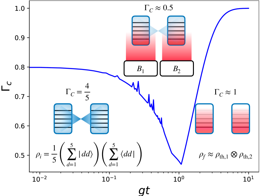
Figure 1: Numerically simulated temporal evolution of the quantum state advantage $\Gamma_{C}(t)$ during thermalization, for two baths $B_{1}$ and $B_{2}$ independently coupling to the qudits, for $D=5$. The insets schematically illustrate the loss of entanglement between the two qudit batteries during the thermalization process (indicated by the weakening of wedge shading between betteries), for various qudit dimensions, cf. Fig. 2.

Initially, at $t=0$, generalized GHZ states are prepared in the two qudits, $|\psi_{0}\rangle=\frac{1}{\sqrt{D}}\sum_{d=1}^{D}|dd\rangle$. They represent maximally entangled states, where $|dd\rangle=|d\rangle\otimes|d\rangle$. The quantum state advantage $\Gamma_{C}(|\psi_{0}\rangle=4/D$ is decreasing with $D$, while the entanglement measure negativity increases with $D$ as ${\mathcal{N}}=0.25(D-1)$.

We illustrate in Fig. 1 that during the thermalization process, with the ensuing loss of entanglement, the quantum state advantage goes through a minimum, but eventually settles at a larger value of $\Gamma_{C}$ than the initial one for the final, completely thermalized and disentangled state for large qudit dimension $D$.

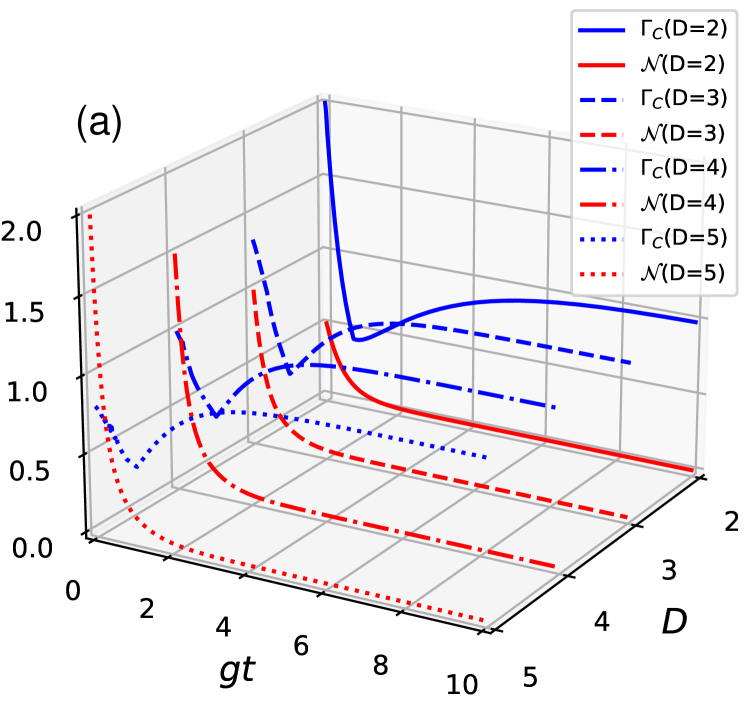
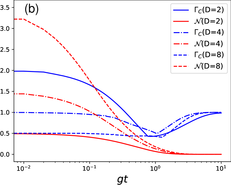
Figure 2: (a) The time evolution of $\Gamma_{C}$ (red) and negativity (red), ${\mathcal{N}}$, via thermalization, for different qudit dimensions $2\leq D\leq 5$, starting from a generalized GHZ state. The thermalization process follows (28). The temperature of the photonic bath is chosen to be small, $k_{B}T=0.1$ relative to the energy gap which we set $\omega_{0}=1$. While negativity monotonically decreases with time $\forall\,D$, the quantum state advantage $\Gamma_{C}$ has a turning point and saturates to unity, and is greater than the initial $\Gamma_{C}=0.8$ (for $D=5$).] (b) Logarithmic representation of time evolution for the quantities displayed in the inset for $D=2,4,8$. Note that the speed of the initial decrease of $\Gamma_{C}$ reduces with qudit dimension and that for $D>4$ the initial $\Gamma_{C}$ is smaller than its final value.

We display the evolution of $\Gamma_{C}$ and $\mathcal{N}$ via the thermalization process by the Lindbladian evolution (28), for various qudit dimensions in Fig. 2. We observe that negativity and thus the entanglement monotonically decrease with time. On the other hand, $\Gamma_{C}$ has turning points where $\Gamma_{C}$ starts to increase and then saturates to unity. This increasing behavior is observed at all dimensions $D$. Indeed, $\Gamma_{C}$ can be small even though large entanglement exists, which suggests that certain kinds of entanglement can deteriorate the maximum quantum battery power. We coin this phenomenon entanglement disadvantage. Indeed, for the present example, when states lose their initially large entanglement quantum disadvantage by thermalization, $\Gamma_{C}$ recuperates to its semiclassical value.

As a conclusion, maximally bipartite-entangled states do not necessarily enhance the quantum charging power, but can potentially act in a detrimental way.

VI.2 Generalized W states

To obtain more concrete examples of the potentially low quantum state advantage of highly entangled states, we use states for which $\Gamma_{C}$ can be calculated analytically. We choose generalized W states Dür et al. (2000), which are commonly referred to as being globally entangled. The W states for $N$ qubits are given by

$$|W_{N}\rangle=\frac{1}{\sqrt{N}}(|100\cdots 0\rangle+|010\cdots 0\rangle+\cdots+|000\cdots 1\rangle).$$ (29)

As shown in Appendix D, we have the exact result $\Gamma_{C}(|W_{N}\rangle)=(3N-2)/N$ [Eq. (LABEL:Gamma_W_N)], which approaches three when $N$ goes to infinity. This clearly suggests that also global entanglement (entanglement connecting all cells) is not a sufficient condition for a quantum-enhanced scaling advantage with the number of cells $N$ (in the large $N$ limit).

VI.3 $k$-local entanglement

We reiterate that although global entanglement is not sufficient for $N$-scaling of the quantum state advantage, global entanglement is still necessary to outperform classical states, i.e., to enhance charging performance. For $k$-local entanglement, which means that each given cell entangles only with at most $k-1$ other cells, we can divide the set of battery cells into partitions composed of $k$ cells which entangle with each other. In this system, $\Gamma_{C}\leq k$ generally, see Eq. (66) in Appendix D, which indicates that there is no quantum state advantage in the sense of a scaling with $N$. As a result, such a quantum state advantage can only stem from a global operator which generates global entanglement, cf. Gyhm et al. (2022). For further discussion see Appendix D.

VI.4 Sachdev-Ye-Kitaev battery charging

A paradigmatic example which has been explicitly demonstrated in Ref. Rossini et al. (2020) to yield a quantum advantage, that is, a power scaling superextensively (faster than linear in $N$), is a charging Hamiltonian of the Sachdev-Ye-Kitaev (SYK) type: Spinless fermions on a lattice, with random all-to-all interactions (see for a review Chowdhury et al. (2022)).

The battery Hamiltonian is here assumed to be a simple magnetic field Hamiltonian

$$\hat{H}=\sum_{i=1}^{N}\mathfrak{h}\sigma^{y}_{i},$$ (30)

where $\sigma^{y}$ is the usual Pauli matrix and $\mathfrak{h}$ is a “magnetic field” with units of energy. This battery is charged by the SYK Hamiltonian,

$$\hat{V}=\sum_{i,j,k,l}J_{ijkl}\hat{c}^{\dagger}_{i}\hat{c}^{\dagger}_{j}\hat{c}_{k}\hat{c}_{l},$$ (31)

where $\hat{c}_{j}^{\dagger}$ and $\hat{c}_{j}$ are creation and annihilation operators of spinless fermions at a given site $j$. By the Jordan-Wigner transformation, the $\hat{c}_{j}$ can be represented by Pauli operators as follows, $\hat{c}_{j}=(\sigma^{x}_{j}-i\sigma^{y}_{j})\prod_{k=1}^{j-1}\sigma^{z}_{k}$, which shows how the SYK charger acts on the battery cells in the $\hat{H}$ of Eq. (30). The interaction coefficients $J_{ijkl}$ are complex random variables, sampled from a Gaussian distribution with zero mean, $f(|J_{ijkl}|)=\sqrt{\bar{J}^{2}/2\pi N^{3}}e^{-N^{3}|J_{ijkl}|^{2}/\bar{J}^{2}}$. The standard deviation reads $\bar{J}/N^{3/2}$, where the $N^{3/2}$ from the normalization guarantees an extensive, that is linear in $N$ scaling of the energy associated to the charging $\hat{V}$.

The initial state is prepared to be the ground state of $\hat{H}$, $\bigotimes_{i=1}^{N}|-Y\rangle_{i}$, with energy $-\mathfrak{h}N$; subsequently, this state is evolved by $\hat{V}$ to a charged state of higher energy. We simulate the corresponding charging process of the SYK battery, to calculate the instantaneous power. To this end, we define a dimensionless time $\tau=t\bar{J}$, and a dimensionless power

$$\tilde{P}(\tau)\coloneqq\ \frac{1}{\sqrt{4\langle\hat{V}^{2}\rangle N\mathfrak{h}^{2}}}P\big{(}\tau\big{)}.$$ (32)

By our theorem 1, the dimensionless power $\tilde{P}$ is in the present case bounded precisely by the square root of the quantum state advantage, $\sqrt{\Gamma_{C}}$. Classical charging, that is by definition charging without generating entanglement, has $\sqrt{\Gamma_{C}}\coloneqq 1$, which thus represents the classical power bound at any time.

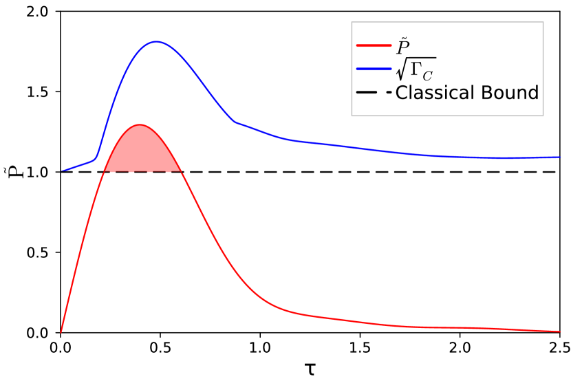
Figure 3: SYK charging. Scaled instantaneous power $\tilde{P}$ as a function of dimensionless time $\tau$ and quantum (blue solid) as well as classical (black dashed) power bounds, for $N=12$ cells. The plot shows one realization of the randomized couplings $J_{ijkl}$; the results for other samplings are very similar. The dashed line shows the classical charging bound corresponding to $\Gamma_{C}=1$.

Fig. 3 plots for one disorder realization the dimensionless power $\tilde{P}$, and dimensionless power bound of our system $\sqrt{\Gamma_{C}}$, both as a function of dimensionless time $\tau$. We verified that other disorder realizations give very similar results, with $\tilde{P}(\tau)$ peaking before its bound $\sqrt{\Gamma_{C}(\tau)}$.

We infer from Fig. 3 that while our power bound is not saturated, the instantaneous power exceeds the classical bound for all times $\tau$ corresponding to the light-red-shaded area in Fig. 3. In this time window, we thus obtain a genuine quantum state advantage from SYK charging.

Furthermore, we observe from Fig. 3 that the quantum state advantage $\Gamma_{C}({\hat{\rho}})$ for a SYK-charged battery is not monotonously increasing with time. The scaled power $\tilde{P}$ returns to unity when the battery quantum state becomes chaotic due to the random couplings of the SYK charger which does maximally entangle the cells Rossini et al. (2020). We prove in Appendix E that a maximally entangled final state has indeed $\Gamma_{C}=1$, and thus no quantum state advantage .

This phenomenon of non-monotonicity of $\Gamma_{C}$, even though the SYK charger maximally entangles, is another instance illustrating our theorem 2, which states that $\Gamma_{C}$ is not an entanglement monotone.

VII Conclusion

To address the entanglement dependence of quantum charging power in a most general, implementation-independent approach, we have employed our novel definition of a commutation matrix instead of the conventionally used covariance matrix. This enables us to isolate the quantum speed limit and the battery energy gap in the bound on the charging power, from the quantum state advantage $\Gamma_{C}({\hat{\rho}})$ which depends only on the quantum state as represented by the density matrix encoding the entanglement. We have thereby, in particular, shown that the maximum obtainable power is not an entanglement monotone. Note that we have also shown (cf. Proposition 3 in Appendix A), that mixtures of product states (separable states), in general leading to quantum correlations beyond entanglement such as for example measured by quantum discord Ollivier and Zurek (2001); Adesso et al. (2016), do not imply a quantum state advantage in the sense we have put forward here. That is, they do not lead to a quantum advantage which is isolable from speed limit and gap.

Indeed, the instantaneous power of battery charging is obviously dependent on the intermediate states between the initial and final states of the charging protocol. Our derived bound then demonstrates the necessity of the entanglement of any intermediate states to gain an instantaneous quantum advantage of battery charging. This statement is, in particular, independent of the preparation of the initial state. We however also again stress that while entanglement is a necessary condition for a quantum state advantage $\Gamma_{C}>1$, we have argued that there also exists a potential quantum disadvantage, that is, highly entangled states can have a potentially lower maximum charging power than separable states, and entanglement is, while necessary, not sufficient to obtain a quantum state advantage.

While we have provided concrete calculations for negativity as a measure of entanglement, we anticipate that the qualitative behavior of the quantum state advantage measure $\Gamma_{C}({\hat{\rho}})$ remains unaffected for other measures of bipartite entanglement. Finally, the generalization to multipartite entanglement measures, and to develop a general classification scheme for beneficially or detrimentally entangled states are left for future study.

Conflict of Interest

The authors have no conflicts to disclose.

Data Availability

The data that support the findings of this study are available from the corresponding author upon reasonable request.

Appendix A Several properties of the commutation matrix

Proposition 1.

$\gamma_{C}({\hat{\rho}},\hat{\bm{M}})$ is a positive semidefinite matrix for any ${\hat{\rho}}$.

Proof.

For any vector ${\bm{u}}$, we can define a corresponding operator $\hat{O}=\hat{\bm{M}}\cdot{\bm{u}}$. By the definition of $\gamma_{C}({\hat{\rho}},\hat{\bm{M}})$ in Eq. (14), we obtain

$$\begin{split}&{\bm{u}}^{\mathrm{T}}\gamma_{C}({\hat{\rho}},\hat{\bm{M}}){\bm{u}}=\sum_{\mu,\nu}u_{\mu}u_{\nu}\gamma_{C}({\hat{\rho}},\hat{\bm{M}})_{\mu\nu}\\ &=-\sum_{\mu,\nu}u_{\mu}u_{\nu}\mathrm{tr}([\hat{M_{\mu}},\sqrt{{\hat{\rho}}}][\hat{M_{\nu}},\sqrt{{\hat{\rho}}}])\\ &=-\mathrm{tr}([\sum_{\mu}u_{\mu}\hat{M_{\mu}},\sqrt{{\hat{\rho}}}][\sum_{\nu}u_{\nu}\hat{M_{\nu}},\sqrt{{\hat{\rho}}}])\\ &=-\mathrm{tr}([\sqrt{{\hat{\rho}}},\hat{O}]^{2}).\end{split}$$ (33)

Both ${\hat{\rho}}$ and $\hat{O}$ are Hermitian operators; then $[\sqrt{{\hat{\rho}}},\hat{O}]$ is an anti-Hermitian operator. Since the eigenvalues of $[\sqrt{{\hat{\rho}}},\hat{O}]$ are imaginary, $[\sqrt{{\hat{\rho}}},\hat{O}]^{2}$ is a negative semidefinite matrix. Hence $-\mathrm{tr}([\sqrt{{\hat{\rho}}},\hat{O}]^{2})$ is zero or positive for any $\hat{O}$ corresponding to a given ${\bm{u}}$, which proves the proposition. ∎

Proposition 2.

The quantum state advantage $\Gamma_{C}({\hat{\rho}})$ is bounded by the number of cells,

$$\Gamma_{C}({\hat{\rho}})\leq N$$ (34)

Proof.

This will be proved by the fact that our inequality (16) is always achievable, and by using Eq. (9).

There always exist some $\hat{H}$ and $\hat{V}$ which satisfy the equality conditions Eqs. (17) and (18). By Eq. (9), we obtain

$$\begin{split}\sqrt{2\kappa\Gamma_{C}({\hat{\rho}})}=\frac{P}{\sqrt{\sum_{i=1}^{N}\mathrm{tr}(\hat{H}_{i}^{2})\langle\Delta\hat{V}^{2}\rangle}}\\ \leq 2\sqrt{\|\gamma({\hat{\rho}},\hat{\bm{M}})\|}\leq\sqrt{2N}.\end{split}$$ (35)

Since $1\leq\kappa\leq 2$, the proposition is proven. ∎

Proposition 3.

For separable states, a linear summation of product states, $\Gamma_{C}({\hat{\rho}})$ is less than or equal to unity; there is no quantum advantage for any such states.

Proof.

The proof is similar to the proof of proposition 2, but here we will use a decomposition of the separable state ${\hat{\rho}}$ as follows.

By the definition of separable states, ${\hat{\rho}}$ can be decomposed by a finite number of product states as

$${\hat{\rho}}=\sum_{l}p_{l}{\hat{\rho}}_{l}.$$ (36)

In this expression, ${\hat{\rho}}_{l}$ can be completely expressed by products of states and $\sum_{l}p_{l}=1$. We can then obtain a bound on the power by Eq. (9),

$$P\leq 2\sum_{l}p_{l}\sqrt{\|\gamma({\hat{\rho}}_{l},\hat{\bm{M}})\|\sum_{i=1}^{N}\mathrm{tr}(\hat{H}_{i}^{2})\langle\Delta V^{2}\rangle_{l}},$$ (37)

where any $\|\gamma({\hat{\rho}}_{l},\hat{\bm{M}})\|$ is equal to 1/2 by definition of the covariance matrix. Using the inequality $\sqrt{\langle\Delta\hat{V}^{2}\rangle}\geq\sum_{l}p_{l}\sqrt{\langle\Delta\hat{V}^{2}\rangle_{l}}$, there always exist $\hat{H}$ and $\hat{V}$ which satisfy the equality conditions in (17) and (18). With Eq. (9), Eq (37)] is rewritten as

$$P\leq\sqrt{2\sum_{i=1}^{N}\mathrm{tr}(\hat{H}_{i}^{2})\langle\Delta V^{2}\rangle},$$ (38)

which yields

$$\sqrt{2\kappa\Gamma_{C}({\hat{\rho}})}=\frac{P}{\sqrt{\sum_{i=1}^{N}\mathrm{tr}(\hat{H}_{i}^{2})\langle\Delta\hat{V}^{2}\rangle}}\leq\sqrt{2}$$ (39)

Since $1\leq\kappa\leq 2$, the proposition is proven. ∎

Proposition 4.

The eigenvalues of $\gamma_{C}({\hat{\rho}})$ are conserved during evolution with local driving Hamiltonians.

Proof.

A local driving Hamiltonian is given as

$$\hat{V}=\sum_{i=1}^{N}\hat{V}_{i}\bigotimes_{j\neq i}\hat{I}_{j},$$ (40)

such that a unitary operator from $\hat{V}$ is expressed by

$$\hat{U}=e^{-i\hat{V}T}=\prod_{i}^{N}e^{-i\hat{V}_{i}\bigotimes_{j\neq i}\hat{I}_{j}}=\prod_{i}^{N}\hat{U}_{i}.$$ (41)

We then obtain the $\gamma_{C}$ matrix for the time-evolved state $\hat{\hat{U}}{\hat{\rho}}\hat{\hat{U}}^{\dagger}$ as follows

$$\begin{split}\gamma_{C}(\hat{U}{\hat{\rho}}\hat{U}^{\dagger},\hat{\bm{M}}_{\mu\nu})=-\mathrm{tr}([\sqrt{\hat{U}{\hat{\rho}}\hat{U}^{\dagger}},\hat{M}_{\mu}][\sqrt{\hat{U}{\hat{\rho}}\hat{U}^{\dagger}},\hat{M}_{\nu}])\\ =-\mathrm{tr}([\sqrt{{\hat{\rho}}},\hat{U}^{\dagger}\hat{M}_{\mu}\hat{U}][\sqrt{{\hat{\rho}}},\hat{U}^{\dagger}\hat{M}_{\nu}\hat{U}]).\end{split}$$ (42)

Without loss of generality, let us assume that $\hat{M}_{\mu}$ derives from the $i$th cell. Then, $\hat{M}_{\mu}$ can be decomposed as $\bigotimes_{j\neq i}\hat{I}^{j}\otimes A^{i}_{\mu}$. By also using the decomposition of $\hat{U}$ into the $\hat{U}_{i}$ according to (41), we can write

$$\hat{U}\bigotimes_{j\neq i}\hat{I}^{j}\otimes A^{i}_{\mu}\hat{U}^{\dagger}=\bigotimes_{j\neq i}\hat{I}^{j}\otimes\hat{U}_{i}A^{i}_{\mu}\hat{U}_{i}^{\dagger},$$ (43)

due to the orthonormality condition (5), $U_{i}A^{i}_{\mu}\hat{U}_{i}^{\dagger}=\sum_{\xi}O_{\mu\xi}A^{i}_{\xi}$ for an orthogonal matrix $O$.

We can expand the orthogonal matrix $O$ using the full space spanned by the $\hat{\bm{M}}$, which leads to $U^{\dagger}\hat{M}_{\mu}U=\sum_{\xi}O_{\mu\xi}\hat{M}_{\xi}$. Hence we can write

$$\gamma_{C}(U{\hat{\rho}}U^{\dagger},\hat{\bm{M}})=O^{\mathrm{T}}\gamma_{C}({\hat{\rho}},\hat{\bm{M}})O.$$ (44)

Therefore the local driving Hamiltonians only act on the state by rotating the basis of the commutation matrix $\gamma_{C}$, and do not change its eigenvalues and hence also its norm, so that $\Gamma_{C}$ is not affected. ∎

Appendix B Proof of inequality (16)

In this Appendix, we will expand on the detailed derivation of Theorem 1, for which the primary steps were outlined in the main text. Let us start with establishing a Cauchy–Schwarz type inequality for operators.

For Hermitian operators $\hat{A}=\sum_{i}a_{i}|a_{i}\rangle\langle a_{i}|$ and $\hat{B}=\sum_{i}b_{i}|b_{i}\rangle\langle b_{i}|$, the following Cauchy-Schwarz type inequality holds:

$$|\mathrm{tr}(\hat{A}\hat{B})|\leq\sqrt{\mathrm{tr}(\hat{A}^{2})\mathrm{tr}(\hat{B}^{2})}$$ (45)

which is derived by an arithmetic geometric-mean inequality as follows

$$\begin{split}&2=\sum_{ij}\left(\frac{a_{i}^{2}}{\mathrm{tr}(\hat{A}^{2})}+\frac{b_{i}^{2}}{\mathrm{tr}(\hat{B}^{2})}\right)|\langle a_{i}|b_{j}\rangle|^{2}\\ &\geq\sum_{ij}\frac{2|a_{i}b_{j}|}{\sqrt{\mathrm{tr}(\hat{A}^{2})\mathrm{tr}(\hat{B}^{2})}}|\langle a_{i}|b_{j}\rangle|^{2}\geq 2\frac{|\mathrm{tr}(\hat{A}\hat{B})|}{\sqrt{\mathrm{tr}(\hat{A}^{2})\mathrm{tr}(\hat{B}^{2})}}.\end{split}$$ (46)

By replacing $\hat{A}$ and $\hat{B}$ in (45) with $i[\hat{H},\sqrt{{\hat{\rho}}}]$ and $\{\sqrt{{\hat{\rho}}},\hat{V}\}$, we obtain the following bound on $P$,

$$|P| = |\mathrm{tr}(i[\hat{H},\sqrt{{\hat{\rho}}}]\{\sqrt{{\hat{\rho}}},\hat{V}\})|$$ (47)

$$\leq \sqrt{\mathrm{tr}(-[\hat{H},\sqrt{{\hat{\rho}}}]^{2})\mathrm{tr}(\{\sqrt{{\hat{\rho}}},\hat{V}\}^{2})},$$

which implies that $\mathrm{tr}(-[{\hat{\rho}},\hat{H}]^{2})$ determines the quantum advantage coming from the state ${\hat{\rho}}$ since we isolated the QSL contribution, encoded in $\{\sqrt{{\hat{\rho}}},\hat{V}\}^{2}$, on the right-hand side of the power inequality, cf. the discussion below Eq. (21).

We now use that the battery Hamiltonian can be written as$\hat{H}=\sqrt{\sum_{i=1}^{N}\mathrm{tr}(\hat{H}_{i}^{2})}\hat{\bm{M}}\cdot{\bm{u}}$ which gives the equality from the definition of $\gamma_{C}({\hat{\rho}},\hat{\bm{M}})$

$$-\mathrm{tr}([{\hat{\rho}},\hat{H}]^{2})=\sum_{i=1}^{N}\mathrm{tr}(\hat{H}_{i}^{2})u^{\mathrm{T}}\gamma_{C}({\hat{\rho}},\hat{\bm{M}})u.$$ (48)

By using the property of the operator norm that it is equal to the largest eigenvalue of the operator, we have the inequality

$$-\mathrm{tr}([{\hat{\rho}},\hat{H}]^{2})\leq\left\|\gamma_{C}({\hat{\rho}},\hat{\bm{M}})\right\|\sum_{i=1}^{N}\mathrm{tr}(H_{i}^{2}).$$ (49)

The quantity $\hat{V}+\lambda\hat{I}$ has identical power $P\,\,\forall\,\lambda$ and $\mathrm{tr}(\{\hat{V}+\lambda\hat{I},\sqrt{{\hat{\rho}}}\})$ is minimized by $2\mathrm{tr}(\sqrt{{\hat{\rho}}}\hat{V}\sqrt{{\hat{\rho}}}\hat{V})+2\mathrm{tr}({\hat{\rho}}\hat{V}^{2})-4\mathrm{tr}({\hat{\rho}}\hat{V})^{2}$ when $\lambda=-\mathrm{tr}(\hat{V}{\hat{\rho}})$.

Since $-\mathrm{tr}([\sqrt{{\hat{\rho}}},\hat{V}]^{2})=2\mathrm{tr}(\sqrt{{\hat{\rho}}}\hat{V}\sqrt{{\hat{\rho}}}\hat{V})-2\mathrm{tr}({\hat{\rho}}\hat{V}^{2})\geq 0$, we can establish the inequality

$$\begin{split}&2\mathrm{tr}(\sqrt{{\hat{\rho}}}\hat{V}\sqrt{{\hat{\rho}}}\hat{V})+2\mathrm{tr}({\hat{\rho}}\hat{V}^{2})-4\mathrm{tr}({\hat{\rho}}\hat{V})^{2}\\ &\leq 4\mathrm{tr}({\hat{\rho}}\hat{V}^{2})-4\mathrm{tr}({\hat{\rho}}\hat{V})^{2}=4\langle\Delta\hat{V}^{2}\rangle.\end{split}$$ (50)

Moreover, $\mathrm{tr}(\sqrt{{\hat{\rho}}}(\hat{V}+\lambda\hat{I})\sqrt{{\hat{\rho}}}(\hat{V}+\lambda\hat{I}))$ is greater or equal to zero $\forall\,\lambda$, so we obtain that $\mathrm{tr}(\sqrt{{\hat{\rho}}}\hat{V}\sqrt{{\hat{\rho}}}\hat{V})-\mathrm{tr}({\hat{\rho}}\hat{V})^{2}\geq 0$. Due to the above inequality (50), $\mathrm{tr}(\{\sqrt{{\hat{\rho}}},\hat{V}\})$ is then bounded by

$$\begin{split}&2\langle\Delta\hat{V}^{2}\rangle=2\mathrm{tr}({\hat{\rho}}\hat{V}^{2})-2\mathrm{tr}({\hat{\rho}}\hat{V})^{2}\\ &\leq 2\mathrm{tr}(\sqrt{{\hat{\rho}}}\hat{V}\sqrt{{\hat{\rho}}}\hat{V})+2\mathrm{tr}({\hat{\rho}}\hat{V}^{2})-4\mathrm{tr}({\hat{\rho}}\hat{V})^{2}.\end{split}$$ (51)

Now we have $\mathrm{tr}(\{\sqrt{{\hat{\rho}}},\hat{V}\}^{2})=2\kappa\langle\Delta\hat{V}^{2}\rangle$ defining a coefficient $\kappa$ which lies in the range $1\leq\kappa\leq 2$.

Consequently, we obtain a power bound in the form

$$P\leq\sqrt{2\kappa\Gamma_{C}({\hat{\rho}})\sum_{i=1}^{N}\mathrm{tr}(\hat{H}_{i}^{2})\langle\Delta\hat{V}^{2}\rangle},$$ (52)

the relation (16) which we set out to prove.

Next we will discuss the condition for a saturation of the bound (16). The equality condition of (45) is $\hat{A}=c\hat{B}$ for an arbitrary real number $c$. Hence the first equality condition (17) arises. The remaining question is which driving Hamiltonian $\hat{V}$ satisfies this condition.

Let us investigate (17) within a density matrix eigenbasis. In this basis, we can write ${\hat{\rho}}=\sum_{\alpha}\rho_{\alpha}|\alpha\rangle\langle\alpha|$, $\hat{H}=\sum_{\alpha\beta}h_{\alpha\beta}|\alpha\rangle\langle\beta|$ and $\hat{V}=\sum_{\alpha\beta}v_{\alpha\beta}|\alpha\rangle\langle\beta|$. Then (17) can be formulated as follows

$$\sum_{\alpha\beta}v_{\alpha\beta}(\sqrt{\rho_{\alpha}}+\sqrt{\rho_{\beta}})|\alpha\rangle\langle\beta|=ic\sum_{\alpha\beta}h_{\alpha\beta}(\sqrt{\rho_{\beta}}-\sqrt{\rho_{\alpha}})|\alpha\rangle\langle\beta|,$$ (53)

for a constant $c=\sqrt{-\mathrm{tr}(\{\sqrt{{\hat{\rho}}},\hat{V}\}^{2})/\mathrm{tr}([\sqrt{{\hat{\rho}}},\hat{H}]^{2})}$. The solutions of (53) are given by

$$v_{\alpha\beta}=ic\frac{\sqrt{\rho_{\beta}}-\sqrt{\rho_{\alpha}}}{\sqrt{\rho_{\alpha}}+\sqrt{\rho_{\beta}}}h_{\alpha\beta}\qquad\forall\,\alpha,\beta.$$ (54)

As a result, there always exist driving $\hat{V}$ satisfying the equality condition (17).

The second equality condition (18) comes from the definition of operator norm. The driving $\hat{H}$ is decomposed in terms of the $\hat{\bm{M}}$ as $\hat{H}=\sqrt{\sum_{i}^{N}\mathrm{tr}(\hat{H}_{i}^{2})}\hat{\bm{M}}\cdot{\bm{u}}$ for real normalized vectors ${\bm{u}}$. By the definition of $\gamma_{C}({\hat{\rho}},\hat{\bm{M}})$, $-\mathrm{tr}([\sqrt{{\hat{\rho}}},\hat{H}]^{2})=(\sum_{i}^{N}\mathrm{tr}(\hat{H}_{i}^{2})){\bm{u}}^{\mathrm{T}}\gamma_{C}({\hat{\rho}},\hat{\bm{M}}){\bm{u}}$. We now use that the operator norm is equal to the maximum absolute value of all eigenvalues of a symmetric real matrix, The commutation matrix $\gamma_{C}({\hat{\rho}},\hat{\bm{M}})$ is such a real symmetric matrix, so there always exists an optimal direction of ${\bm{u}}={\bm{u}}_{m}$ projecting out the largest eigenvalue of $\gamma_{C}$, which finally gives

$$\begin{split}-\mathrm{tr}([\sqrt{{\hat{\rho}}},\hat{H}]^{2})&=(\sum_{i}^{N}\mathrm{tr}(\hat{H}_{i}^{2})){\bm{u}}_{m}^{\mathrm{T}}\gamma_{C}({\hat{\rho}},\hat{\bm{M}}){\bm{u}}_{m}\\ &=(\sum_{i}^{N}\mathrm{tr}(\hat{H}_{i}^{2}))\Gamma_{C}({\hat{\rho}})\end{split}$$ (55)

Now we established the second equality condition (18) and the fact that it is always achievable for any ${\hat{\rho}}$.

Appendix C Proof of equation (26)

In Appendix B, we proved that our inequality for the power can be saturated by manipulating the battery driving Hamiltonians, $\hat{H}$ and $\hat{V}$, respectively. However, we can not access all kinds of Hamiltonians; we only have a restricted choice of Hamiltonians, which renders the bound on the power (16) loose.

To quantify how loose our bound actually is, we define two angles $\theta_{\hat{H}}$ and $\theta_{\hat{V}}$, by Eqs. (24) and (25). By substituting $\theta_{\hat{H}}$ and $\theta_{\hat{V}}$ into Eq. (26), we can confirm it is identically fulfilled. We bring Eq. (26) into the form

$$P=\sqrt{2\kappa\Gamma_{C}({\hat{\rho}})\sum_{i=1}^{N}\mathrm{tr}(\hat{H}_{i}^{2})\langle\Delta\hat{V}^{2}\rangle\cos{\theta_{\hat{V}}}\cos{\theta_{\hat{H}}}}.$$ (56)

By the definition of $\theta_{\hat{H}}$, we obtain that Eq. (56) is equivalent to

$$P=\sqrt{-2\kappa\mathrm{tr}([\hat{H},\sqrt{{\hat{\rho}}}]^{2})\langle\Delta\hat{V}^{2}\rangle\cos{\theta_{\hat{V}}}}.$$ (57)

Because $\kappa$ is defined by $\mathrm{tr}(\{\sqrt{{\hat{\rho}}},\hat{V}\}^{2})/2\langle\Delta\hat{V}^{2}\rangle$, the Eq. (57) can be represented as

$$P=\sqrt{-\mathrm{tr}([\hat{H},\sqrt{{\hat{\rho}}}]^{2})\mathrm{tr}(\{\sqrt{{\hat{\rho}}},\hat{V}\}^{2})\cos{\theta_{\hat{V}}}},$$ (58)

which is, as required, identically true:

$$\mathrm{tr}(i[\hat{H},\sqrt{{\hat{\rho}}}]\{\sqrt{{\hat{\rho}}},\hat{V}\})=\mathrm{tr}(i\hat{H}[{\hat{\rho}},\hat{V}])\coloneqq P,$$ (59)

by using the definition of $\theta_{\hat{V}}$ and the cyclic property of the trace.

Appendix D Quantum state advantage $\Gamma_{C}$ for W and $k$-locally entangled states

In the main text, we have provided the quantum advantage of pure states for several examples. We detail here the corresponding derivations.

D.1 W states

We first prove for generalized W states that $\Gamma_{C}(|W_{N}\rangle)$ is the function $\Gamma_{C}(|W_{N}\rangle)=(3N-1)/N$. Since W states only occupy a finite number of $N$ Fock space states, this can be analytically derived. The orthonormal set (6) for noninteracting batteries is given by ($1\leq i,j\leq N$)

$$\begin{split}\hat{\bm{M}}=\left\{\frac{1}{\sqrt{2}}\sigma_{i}^{x}\bigotimes_{j\neq i}\hat{I}_{j},\frac{1}{\sqrt{2}}\sigma_{i}^{y}\bigotimes_{j\neq i}\hat{I}_{j},\frac{1}{\sqrt{2}}\sigma_{i}^{z}\bigotimes_{j\neq i}\hat{I}_{j},\frac{1}{\sqrt{2}}\hat{I}_{i}\bigotimes_{j\neq i}\hat{I}_{j}\right\}.\end{split}$$ (60)

We define a set of matrices $\gamma^{\sigma}(1\leq\sigma\leq 4)$ as follows

$$\gamma^{\sigma}_{ij}\vcentcolon=\gamma_{C}(|W_{N}\rangle,\hat{\bm{M}})_{3i+\sigma,3j+\sigma},$$ (61)

where the $i,j=1,\ldots,N$ are site indices as previously. We then have $\gamma_{C}(|W_{N}\rangle,\hat{\bm{M}})=\gamma^{1}\bigoplus\gamma^{2}\bigoplus\gamma^{3}\bigoplus\gamma^{4}$, since the $\gamma_{C}(|W_{N}\rangle,\hat{\bm{M}})_{3i+k,3j+l}$ vanish $\forall\,i,j$ when $k\neq l$.

The four matrices $\gamma^{\sigma}$ have the following elements

$$\gamma^{1}_{ij}=\gamma^{2}_{ij}= \begin{cases}1\quad&\mathrm{for\,\,}i=j\\ \frac{2}{N}\quad&\mathrm{for}\,\,i\neq j\end{cases},\quad\qquad\gamma^{3}_{ij}=\begin{cases}\frac{4N-4}{N^{2}}\quad&\mathrm{for}\,i=j\\ \frac{4}{N^{2}}\quad&\mathrm{for}\,i\neq j\end{cases},\qquad\quad\gamma^{4}_{ij}=0,$$ (62)

from which we can readily obtain their eigenvalues. By the definition of $\Gamma_{C}$, it then follows

$$\begin{split}&\Gamma_{C}(|W_{N}\rangle)=\|\gamma_{C}(|W_{N}\rangle,\hat{\bm{M}})\|\\ &=\max(\|\gamma^{1}\|,\|\gamma^{2}\|,\|\gamma^{3}\|)=\frac{3N-2}{N}.\end{split}$$ (63)

We have confirmed this analytical result by direct numerical evaluation of $\Gamma_{C}(|W_{N}\rangle)$.

D.2 $k$-locally entangled states

As stated in the main text, a $k$-local entangled system is divided into partitions in which at most $k$ cells are entangled within each partition, but the cell states in different partitions are not entangled among each other. Formally, this assumption on the locality of entanglement is therefore expressed as

$$|\psi\rangle=\bigotimes_{p=1}^{P}|\psi_{p}\rangle,$$ (64)

where all $|\psi_{p}\rangle$ are composed from $k$ cells at most and $p$ labels all possible partitions.

In the present case, $\gamma_{C}(\psi)$ can be represented by a simple sum of the commutation matrices from each partition,

$$\gamma_{C}(\psi)=\bigoplus_{p=1}^{P}\gamma_{C}(\psi_{p}),$$ (65)

because of the given assumption that there is no entanglement between cells from different partitions. We finally obtain

$$\Gamma_{C}(|\psi\rangle)=\|\gamma_{C}(|\psi\rangle)\|=\max_{p}\|\gamma_{C}(|\psi_{p}\rangle)\|\leq k,$$ (66)

since each $\|\gamma_{C}(|\psi_{p}\rangle)\|$ is less than or equal to the number of cells in the given partition.

Appendix E Maximally entangled quantum chaos implies $\Gamma_{C}=1$

The SYK charging operator generates many-body chaos with a large amount of entanglement Kobrin et al. (2021). We assume in the following that the final chaotic states, $|\psi_{C}\rangle$ have maximal entanglement entropy for any partition, such that the entanglement entropy for the partition $A$, which has a $d_{A}$-dimensional Hilbert space, reads

$$-\mathrm{tr}({\hat{\rho}}_{A}\ln({\hat{\rho}}_{A}))=\ln(d_{A}),$$ (67)

with the reduced density matrix, traced over the complement of $A$

$${\hat{\rho}}_{A}=\mathrm{tr}_{\neg A}(|\psi_{C}\rangle\langle\psi_{C}|).$$ (68)

To maximize the entanglement entropy, the mixed state, ${\hat{\rho}}_{A}$ should be a maximally mixed state, such that

$${\hat{\rho}}_{A}=\hat{I}/d_{A}.$$ (69)

This implies that a mixed state for a given single cell has density matrix ${\hat{\rho}}_{i}=\hat{I}/2$ and a mixed state for two cells has ${\hat{\rho}}_{ij}=\hat{I}/4\,\forall i\neq j$ since the cells in our case are qubits.

By definition $\hat{M}_{\mu}$ is an element of $\hat{\bm{M}}^{i}$ for some $1\leq i\leq N$. Hence, we can assume $\hat{M}_{\mu}=\hat{A}_{\alpha}^{i}\bigotimes_{k\neq i}\hat{I}^{k}$ and $\hat{M}_{\nu}=\hat{A}_{\beta}^{j}\bigotimes_{k\neq j}\hat{I}^{k}$ without loss of generality. When $i\neq j$, we obtain that

$$\begin{split}\gamma_{C}(|\psi_{C}\rangle\langle\psi_{C}|,\hat{\bm{M}})_{\mu\nu}\!\!=\!\mathrm{tr}([\hat{M_{\mu}},|\psi_{C}\rangle\langle\psi_{C}|][\hat{M_{\nu}},|\psi_{C}\rangle\langle\psi_{C}|]),\end{split}$$ (70)

because of the pure state property $\sqrt{|\psi_{C}\rangle\langle\psi_{C}|}=|\psi_{C}\rangle\langle\psi_{C}|$. We trace out all sites $k\neq i,j$, which yields

$$\begin{split}\gamma_{C}(|\psi_{C}\rangle\langle\psi_{C}|,\hat{\bm{M}})_{\mu\nu}\!=2\mathrm{tr}(\hat{A}_{\alpha}^{i}\otimes\hat{A}_{\beta}^{j}{\hat{\rho}}_{ij})\\ -2\mathrm{tr}(\hat{A}_{\alpha}^{i}\otimes\hat{I}^{j}{\hat{\rho}}_{ij})\mathrm{tr}(\hat{I}^{i}\otimes\hat{A}_{\beta}^{j}{\hat{\rho}}_{ij})\end{split}$$ (71)

By using our assumption (69), ${\hat{\rho}}_{ij}=\hat{I}/4$, Eq. (71) becomes

$$\begin{split}&\gamma_{C}(|\psi_{C}\rangle\langle\psi_{C}|,\hat{\bm{M}})_{\mu\nu}\\ &=\mathrm{tr}(\hat{A}_{\alpha}^{i}\otimes\hat{A}_{\beta}^{j})/2-\mathrm{tr}(\hat{A}_{\alpha}^{i}\otimes\hat{I}^{j})\mathrm{tr}(\hat{I}^{i}\otimes\hat{A}_{\beta}^{j})/2=0.\end{split}$$ (72)

When $i=j$, we trace out all $k\neq i$ such that

$$\begin{split}\gamma_{C}(|\psi_{C}\rangle\langle\psi_{C}|,\hat{\bm{M}})_{\mu\nu}\!=\!2\mathrm{tr}(\hat{A}_{\alpha}^{i}\hat{A}_{\beta}^{i}{\hat{\rho}}_{i})\!-2\mathrm{tr}(\hat{A}_{\alpha}^{i}{\hat{\rho}}_{i})\mathrm{tr}(\hat{A}_{\beta}^{i}{\hat{\rho}}_{i}).\end{split}$$ (73)

By using the assumption (69), ${\hat{\rho}}_{i}=\hat{I}/2$,

$$\begin{split}\gamma_{C}(|\psi_{C}\rangle\langle\psi_{C}|,\hat{\bm{M}})_{\mu\nu}\!=2\mathrm{tr}(\hat{A}_{\alpha}^{i}\hat{A}_{\beta}^{i})-\mathrm{tr}(\hat{A}_{\alpha}^{i})\mathrm{tr}(\hat{A}_{\beta}^{i}),\end{split}$$ (74)

which identically vanishes when $\alpha\neq\beta$ by the orthogonality condition (5) fulfilled by the $\hat{A}_{\alpha}$.

Now the $\alpha=\beta$ case remains to be assessed. For a two-level system, the set of the $\hat{A}_{\alpha}$ is composed of normalized Pauli matrices, $\sigma_{i}^{x}/\sqrt{2},\sigma^{y}/\sqrt{2},\sigma^{z}/\sqrt{2}$ and the identity operator $\hat{I}/\sqrt{2}$. When $\hat{A}_{\alpha}^{i}$ is a normalized Pauli matrix, Eq. (74) yields unity and it gives zero for $\hat{A}_{\alpha}^{i}=\hat{I}/\sqrt{2}$.

Consequently, $\gamma_{C}(|\psi_{C}\rangle\langle\psi_{C}|,\hat{\bm{M}})_{\mu\nu}$ is a diagonal matrix with elements unity or zero. Hence $\Gamma_{C}{|\psi_{C}\rangle\langle\psi_{C}|}=\|\gamma_{C}(|\psi_{C}\rangle\langle\psi_{C}|,\hat{\bm{M}})_{\mu\nu}\|$ is equal to unity, which proves the assertion stated in the section header.

References

- et al. (2020) Han-Sen Zhong et al., “Quantum computational advantage using photons,” Science 370, 1460–1463 (2020).
- Madsen et al. (2022) Lars S. Madsen et al., “Quantum computational advantage with a programmable photonic processor,” Nature 606, 75–81 (2022).
- Giovannetti et al. (2004) Vittorio Giovannetti, Seth Lloyd, and Lorenzo Maccone, “Quantum-Enhanced Measurements: Beating the Standard Quantum Limit,” Science 306, 1330–1336 (2004).
- Braun et al. (2018) Daniel Braun, Gerardo Adesso, Fabio Benatti, Roberto Floreanini, Ugo Marzolino, Morgan W. Mitchell, and Stefano Pirandola, “Quantum-enhanced measurements without entanglement,” Rev. Mod. Phys. 90, 035006 (2018).
- Collaboration (2011) The LIGO Scientific Collaboration, “A gravitational wave observatory operating beyond the quantum shot-noise limit,” Nature Physics 7, 962–965 (2011).
- Gisin et al. (2002) Nicolas Gisin, Grégoire Ribordy, Wolfgang Tittel, and Hugo Zbinden, “Quantum cryptography,” Rev. Mod. Phys. 74, 145–195 (2002).
- Gisin and Thew (2007) Nicolas Gisin and Rob Thew, “Quantum communication,” Nature Photonics 1, 165–171 (2007).
- Auffèves (2022) Alexia Auffèves, “Quantum Technologies Need a Quantum Energy Initiative,” PRX Quantum 3, 020101 (2022).
- Binder et al. (2015) Felix C. Binder, Sai Vinjanampathy, Kavan Modi, and John Goold, “Quantacell: powerful charging of quantum batteries,” New Journal of Physics 17, 075015 (2015).
- Campaioli et al. (2017) Francesco Campaioli, Felix A. Pollock, Felix C. Binder, Lucas Céleri, John Goold, Sai Vinjanampathy, and Kavan Modi, “Enhancing the Charging Power of Quantum Batteries,” Phys. Rev. Lett. 118, 150601 (2017).
- Campaioli et al. (2018) Francesco Campaioli, Felix A. Pollock, and Sai Vinjanampathy, “Quantum Batteries,” in Fundamental Theories of Physics (Springer International Publishing, 2018) pp. 207–225.
- Carrasco et al. (2022) Javier Carrasco, Jerónimo R. Maze, Carla Hermann-Avigliano, and Felipe Barra, “Collective enhancement in dissipative quantum batteries,” Phys. Rev. E 105, 064119 (2022).
- Rossini et al. (2020) Davide Rossini, Gian Marcello Andolina, Dario Rosa, Matteo Carrega, and Marco Polini, “Quantum Advantage in the Charging Process of Sachdev-Ye-Kitaev Batteries,” Phys. Rev. Lett. 125, 236402 (2020).
- Gyhm et al. (2022) Ju-Yeon Gyhm, Dominik Šafránek, and Dario Rosa, “Quantum Charging Advantage Cannot Be Extensive without Global Operations,” Phys. Rev. Lett. 128, 140501 (2022).
- Alicki and Fannes (2013) Robert Alicki and Mark Fannes, “Entanglement boost for extractable work from ensembles of quantum batteries,” Phys. Rev. E 87, 042123 (2013).
- Hovhannisyan et al. (2013) Karen V. Hovhannisyan, Martí Perarnau-Llobet, Marcus Huber, and Antonio Acín, “Entanglement Generation is Not Necessary for Optimal Work Extraction,” Phys. Rev. Lett. 111, 240401 (2013).
- García-Pintos et al. (2020) Luis Pedro García-Pintos, Alioscia Hamma, and Adolfo del Campo, “Fluctuations in Extractable Work Bound the Charging Power of Quantum Batteries,” Phys. Rev. Lett. 125, 040601 (2020).
- Barra (2019) Felipe Barra, “Dissipative Charging of a Quantum Battery,” Phys. Rev. Lett. 122, 210601 (2019).
- Shi et al. (2022) Hai-Long Shi, Shu Ding, Qing-Kun Wan, Xiao-Hui Wang, and Wen-Li Yang, “Entanglement, Coherence, and Extractable Work in Quantum Batteries,” Phys. Rev. Lett. 129, 130602 (2022).
- Šafránek et al. (2023) Dominik Šafránek, Dario Rosa, and Felix C. Binder, “Work Extraction from Unknown Quantum Sources,” Phys. Rev. Lett. 130, 210401 (2023).
- Bhattacharjee and Dutta (2021) Sourav Bhattacharjee and Amit Dutta, “Quantum thermal machines and batteries,” The European Physical Journal B 94, 239 (2021).
- et al. (2022a) James Q. Quach et al., “Superabsorption in an organic microcavity: Toward a quantum battery,” Science Advances 8, eabk3160 (2022a).
- et al. (2022b) Chang-Kang Hu et al., “Optimal charging of a superconducting quantum battery,” Quantum Science and Technology 7, 045018 (2022b).
- Joshi and Mahesh (2022) Jitendra Joshi and T. S. Mahesh, “Experimental investigation of a quantum battery using star-topology NMR spin systems,” Phys. Rev. A 106, 042601 (2022).
- Cruz et al. (2022) Clebson Cruz, Maron F. Anka, Mario S. Reis, Romain Bachelard, and Alan C. Santos, “Quantum battery based on quantum discord at room temperature,” Quantum Science and Technology 7, 025020 (2022).
- Andolina et al. (2019) Gian Marcello Andolina, Maximilian Keck, Andrea Mari, Vittorio Giovannetti, and Marco Polini, “Quantum versus classical many-body batteries,” Physical Review B 99, 205437 (2019).
- Ferraro et al. (2018) Dario Ferraro, Michele Campisi, Gian Marcello Andolina, Vittorio Pellegrini, and Marco Polini, “High-Power Collective Charging of a Solid-State Quantum Battery,” Phys. Rev. Lett. 120, 117702 (2018).
- Julià-Farré et al. (2020) Sergi Julià-Farré, Tymoteusz Salamon, Arnau Riera, Manabendra N. Bera, and Maciej Lewenstein, “Bounds on the capacity and power of quantum batteries,” Phys. Rev. Research 2, 023113 (2020).
- Kamin et al. (2020) F. H. Kamin, F. T. Tabesh, S. Salimi, and Alan C. Santos, “Entanglement, coherence, and charging process of quantum batteries,” Phys. Rev. E 102, 052109 (2020).
- Le et al. (2018) Thao P. Le, Jesper Levinsen, Kavan Modi, Meera M. Parish, and Felix A. Pollock, “Spin-chain model of a many-body quantum battery,” Phys. Rev. A 97, 022106 (2018).
- Gühne et al. (2007) O. Gühne, P. Hyllus, O. Gittsovich, and J. Eisert, “Covariance Matrices and the Separability Problem,” Phys. Rev. Lett. 99, 130504 (2007).
- Li et al. (2008) Ming Li, Shao-Ming Fei, and Zhi-Xi Wang, “Separability and entanglement of quantum states based on covariance matrices,” Journal of Physics A: Mathematical and Theoretical 41, 202002 (2008).
- Gittsovich and Gühne (2010) Oleg Gittsovich and Otfried Gühne, “Quantifying entanglement with covariance matrices,” Phys. Rev. A 81, 032333 (2010).
- Hassani (2013) S. Hassani, Mathematical Physics: A Modern Introduction to Its Foundations (Springer International Publishing, 2013).
- Deffner and Campbell (2017) Sebastian Deffner and Steve Campbell, “Quantum speed limits: from Heisenberg’s uncertainty principle to optimal quantum control,” Journal of Physics A: Mathematical and Theoretical 50, 453001 (2017).
- Nielsen (1999) M. A. Nielsen, “Conditions for a Class of Entanglement Transformations,” Phys. Rev. Lett. 83, 436–439 (1999).
- Bennett et al. (1999) Charles H. Bennett, David P. DiVincenzo, Christopher A. Fuchs, Tal Mor, Eric Rains, Peter W. Shor, John A. Smolin, and William K. Wootters, “Quantum nonlocality without entanglement,” Phys. Rev. A 59, 1070–1091 (1999).
- Vidal (2000) Guifré Vidal, “Entanglement monotones,” Journal of Modern Optics 47, 355–376 (2000).
- Vidal and Werner (2002) G. Vidal and R. F. Werner, “Computable measure of entanglement,” Phys. Rev. A 65, 032314 (2002).
- Breuer and Petruccione (2007) Heinz-Peter Breuer and Francesco Petruccione, The Theory of Open Quantum Systems (Oxford University Press, 2007).
- Dür et al. (2000) W. Dür, G. Vidal, and J. I. Cirac, “Three qubits can be entangled in two inequivalent ways,” Phys. Rev. A 62, 062314 (2000).
- Chowdhury et al. (2022) Debanjan Chowdhury, Antoine Georges, Olivier Parcollet, and Subir Sachdev, “Sachdev-Ye-Kitaev models and beyond: Window into non-Fermi liquids,” Rev. Mod. Phys. 94, 035004 (2022).
- Note (1) We conjecture in this regard that the asymptotics of the bound (solid blue line in Fig. 3) apparently not reaching unity is a finite effect ( in our simulations).
- Ollivier and Zurek (2001) Harold Ollivier and Wojciech H. Zurek, “Quantum Discord: A Measure of the Quantumness of Correlations,” Phys. Rev. Lett. 88, 017901 (2001).
- Adesso et al. (2016) Gerardo Adesso, Thomas R. Bromley, and Marco Cianciaruso, “Measures and applications of quantum correlations,” Journal of Physics A: Mathematical and Theoretical 49, 473001 (2016).
- Kobrin et al. (2021) Bryce Kobrin, Zhenbin Yang, Gregory D. Kahanamoku-Meyer, Christopher T. Olund, Joel E. Moore, Douglas Stanford, and Norman Y. Yao, “Many-Body Chaos in the Sachdev-Ye-Kitaev Model,” Phys. Rev. Lett. 126, 030602 (2021).