Entangled time-crystal phase in an open quantum light-matter system

Abstract

Time-crystals are nonequilibrium many-body phases in which the state of the system dynamically approaches a limit cycle. While these phases are recently in the focus of intensive research, it is still far from clear whether they can host quantum correlations. In fact, mostly classical correlations have been observed so far and time-crystals appear to be effectively classical high-entropy phases. Here, we consider the nonequilibrium behavior of an open quantum light-matter system, realizable in current experiments, which maps onto a paradigmatic time-crystal model after an adiabatic elimination of the light field. The system displays a bistable regime, with coexistent time-crystal and stationary phases, terminating at a tricritical point from which a second-order phase transition line departs. While light and matter are uncorrelated in the stationary phase, the time-crystal phase features bipartite correlations, both of quantum and classical nature. Our work unveils that time-crystal phases in collective open quantum systems can sustain quantum correlations, including entanglement, and are thus more than effectively classical many-body phases.

Interacting light-matter systems can feature intriguing collective behavior and phase transitions. An example is given by transitions into superradiant phases, i.e., phases with a “macroscopically” excited light field [1, 2, 3, 4, 5, 6, 7, 8, 9, 10, 11]. In the presence of Markovian dissipation, these systems generically approach, at long times, a stationary state. However, under certain conditions, genuine dynamical regimes may occur [12], as it happens, for instance, in the case of lasing [13] or counter-lasing regimes [14, 15, 16, 17, 18]. The emergence of non-stationary many-body behavior [19, 20, 21, 22, 23], with the system undergoing persistent oscillatory dynamics, witnesses the breaking of the continuous time-translation symmetry of the dynamical generator and the concomitant formation of a crystalline structure in time. Because of this reason, these nonequilibrium phases are referred to as time-crystals (see, e.g., Refs. [24, 25, 26, 27, 28, 29, 30, 31, 32, 33, 34, 23, 35]).

A minimal Markovian open quantum system displaying non-stationary behavior is the so-called boundary time-crystal [19], generalized in Refs. [36, 37, 38, 39] and experimentally realized in Ref. [40]. It consists of a collective many-body spin model which allows for both efficient numerical simulations [41, 42, 43, 44, 45, 46] and exact analytical solutions [47, 48, 49, 36, 50, 51, 52]. This model features quantum correlations in its stationary phase — witnessed by non-zero spin-squeezing and two-qubit entanglement — but only classical correlations in the time-crystal regime [53, 36, 50, 51, 54, 55, 56], which is described by highly mixed and effectively classical states [37, 50, 51, 57]. It thus remains an open question whether (boundary) time-crystal phases can host quantum effects or whether these phases are essentially purely classical dynamical regimes.

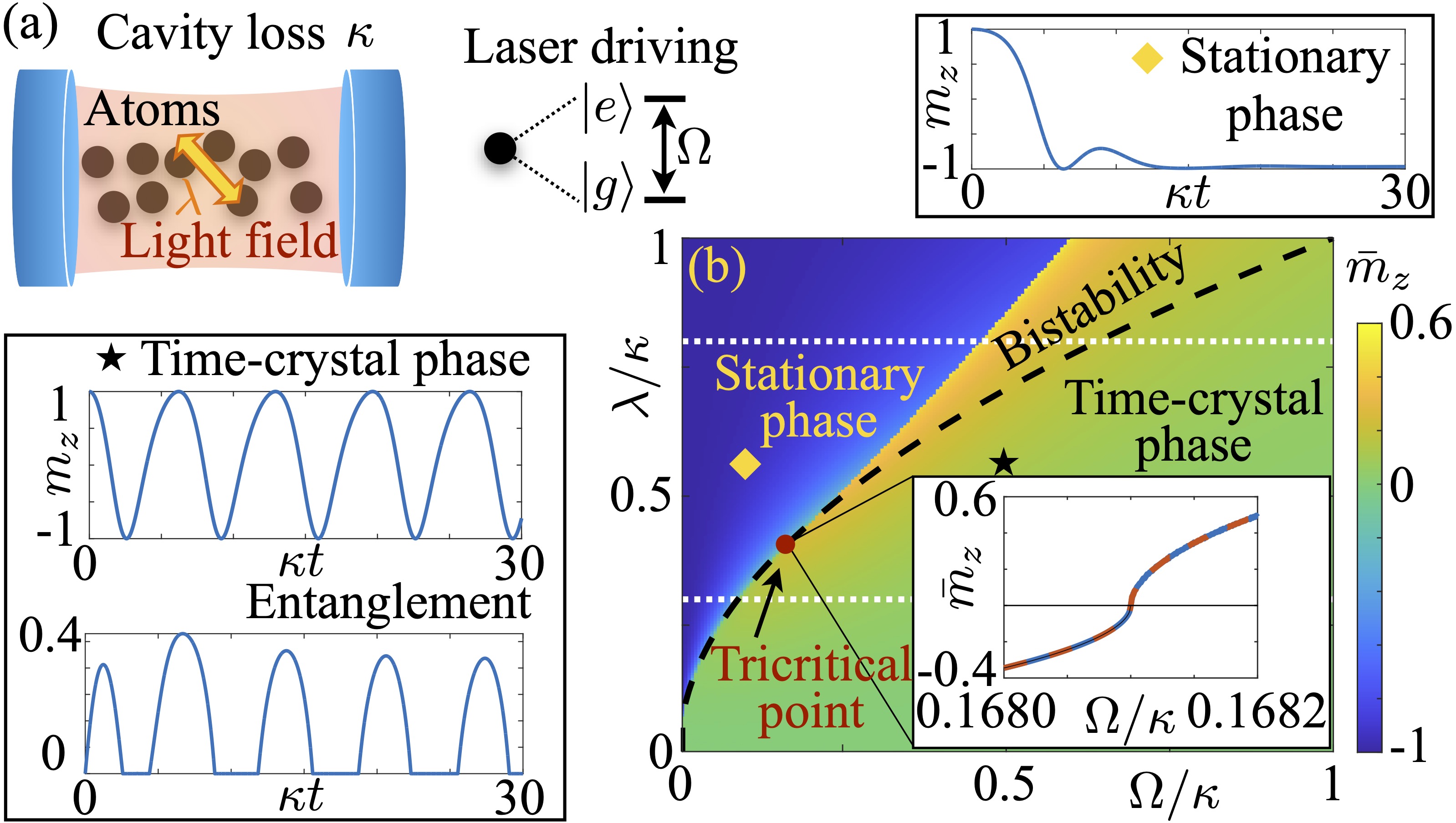
Figure 1: System and nonequilibrium phase diagram. (a) An ensemble of two-level atoms, with ground state $\ket{g}$ and excited state $\ket{e}$, is driven by a laser with Rabi-frequency $\Omega$ and interacts via exchange of excitations with the light field of a cavity (coupling constant $\lambda$). The cavity is also subject to photon loss at rate $\kappa$. (b) The time-averaged magnetization $\bar{m}_{z}$, defined through the states $\ket{g},\ket{e}$, as a function of $\Omega$ and $\lambda$ shows the emergence of a phase transition. One phase is stationary (see behavior of the magnetization $m_{z}$ as a function of time in the upper inset), while the other one is a time-crystal, in which the system undergoes persistent oscillations (see left inset). The phase diagram features a bistable regime which terminates at a tricritical point, $(\Omega/\kappa,\lambda/\kappa)\approx(0.17,0.41)$. Here, the transition becomes of second order (see inset). The time-crystal phase features collective entanglement between the atoms and the light field. Below the dashed line, the system does not possess a well-defined stationary state.

In this paper, we consider a paradigmatic model describing atoms coupled to a light field via an excitation-exchange interaction [58, 59, 60, 61], see sketch in Fig. 1(a). This system can be realized in current cavity-atom experiments [62, 63, 64, 65, 66, 67, 68, 69] and realizes a boundary time-crystal [70, 71, 72, 60] when adiabatically eliminating the light field. It features both a stationary superradiant and a time-crystal phase [61]. Within the parameter regime in which one may expect the adiabatic elimination to hold, the nonequilibrium transition between the two phases is a second-order one. However, in contrast to the boundary time-crystal, the system features a bistable regime, characterized by the coexistence of a limit cycle and a stationary phase. This signals that the phase transition eventually becomes of first order [cf. Fig. 1(b)]. Explicitly taking into account the light field further allows us — to best of our knowledge for the first time — to observe the emergence of quantum correlations, including entanglement, in a time-crystal regime. The existence of these correlations may motivate the development of alternative strategies for exploiting these phases for enhanced metrological applications [55, 56].

The system.— We consider a driven-dissipative version of the so-called Tavis-Cummings spin-boson model [58, 59, 13, 69]. For concreteness, we focus on a realization of the model in a cavity setup, as depicted in Fig. 1(a). The spins describe $N$ two-level atoms with ground state $\ket{g}$, excited state $\ket{e}$, and energy splitting $\omega_{\rm at}$. The bosonic operators $a,a^{\dagger}$ are associated with the light field inside the cavity (frequency $\omega_{\rm cav}=\omega_{\rm at}$). For later convenience, we define the quadrature operators $q=i(a-a^{\dagger})/\sqrt{2}$ and $p=(a+a^{\dagger})/\sqrt{2}$, such that $[q,p]=i$.

The atoms are resonantly driven by a laser and, in the rotating frame, the system Hamiltonian is given by

$$H=\Omega(S_{+}+S_{-})+\frac{\lambda}{\sqrt{N}}\left(a^{\dagger}S_{-}+aS_{+}\right)\,,$$ (1)

with $\Omega$ being the laser Rabi-frequency and $\lambda$ the coupling constant providing the “rate” of the coherent exchange of excitations. The collective atom operators $S_{\pm}$ are defined as $S_{-}=\sum_{k=1}^{N}\sigma_{-}^{(k)}$, with $\sigma_{-}=\ket{g}\!\bra{e}$, $S_{+}=S_{-}^{\dagger}$. The factor $1/\sqrt{N}$ in front of the coupling term ensures a well-defined thermodynamic limit [13, 73]. Photon losses, at rate $\kappa$, are described by the dissipator [74, 75]

$$\mathcal{L}[X]=\kappa\left(aXa^{\dagger}-\frac{1}{2}\left\{a^{\dagger}a,X\right\}\right)\,.$$ (2)

The full quantum state of the system, $\rho$, thus evolves according to the quantum master equation $\dot{\rho}_{t}=-i[H,\rho_{t}]+\mathcal{L}[\rho_{t}]$ and allows for the calculation of the expectation value of any operator $O$, as $\langle O\rangle_{t}:={\rm Tr}(\rho_{t}O)$.

While the Tavis-Cummings model [58, 59] has been considered in several works [76, 77, 78, 79, 63, 65, 80, 81, 82, 83, 84, 85, 86, 87, 88, 89], the setting analyzed here appears to be not much explored [61], and even less for what concerns the analysis of quantum correlations (see related studies in Refs. [90, 91, 92, 93]), mostly investigated in the few-atom case [94, 95, 96, 97, 98, 99, 100, 101, 102, 103, 104, 105, 106].

Time-crystal phase.— To demonstrate the emergence of a phase characterized by non-stationary asymptotic dynamics, we analyze the long-time behavior of our system, in the thermodynamic limit ($N\to\infty$). To this end, we introduce the average “magnetization” operators $m^{N}_{r}=\sum_{k=1}^{N}\sigma_{r}^{(k)}/N$ for the atoms, with $\sigma_{r}$ being the Pauli matrices constructed from the states $\ket{g}$ and $\ket{e}$. For the light field, we consider the rescaled quadratures $m_{q}^{N}=q/\sqrt{N}$ and $m_{p}^{N}=p/\sqrt{N}$. In the thermodynamic limit, both the atom and the light-field operators $m_{r}=\lim_{N\to\infty}m_{r}^{N}$ describe average properties of the system [73, 51] and provide suitable order parameters.

Since we are interested in the long-time regime, we derive the evolution equations for the average operators. We focus on physically-relevant initial states [107], i.e., states with sufficiently short-range correlations. The order-parameter dynamics is thus exactly captured by a set of nonlinear differential equations [73, 108, 109]. [110, 111, 112, 113] For our system, the latter shows that $m_{x}^{2}+m_{y}^{2}+m_{z}^{2}$ is a constant of motion, which we set to one, and that assuming an initial state for which $m_{x}(0)=m_{q}(0)=0$, results in having $m_{x}(t)=m_{q}(t)=0$, for all times $t>0$. The remaining operators evolve via the equations [109]

$$\begin{split}\dot{m}_{y}(t)&=-2\Omega m_{z}(t)-\sqrt{2}\lambda m_{p}(t)m_{z}(t)\,,\\ \dot{m}_{z}(t)&=2\Omega m_{y}(t)+\sqrt{2}\lambda m_{p}(t)m_{y}(t)\,,\\ \dot{m}_{p}(t)&=-\frac{\lambda}{\sqrt{2}}m_{y}(t)-\frac{\kappa}{2}m_{p}(t)\,.\end{split}$$ (3)

We note that, adiabatically eliminating $m_{p}(t)$, by setting the last of the equations above to zero and substituting the result in the other two equations, leads to the equations of motion for the boundary time-crystal model [19, 51]. A similar mapping holds also at an operatorial level [60]. The above system of equations features two stationary solutions, only one of which,

$$m_{y}^{*}=\frac{\Omega\kappa}{\lambda^{2}}\,,\,m_{z}^{*}=-\sqrt{1-\left(\frac{\Omega\kappa}{\lambda^{2}}\right)^{2}}\,,\,m_{p}^{*}=-\frac{\sqrt{2}\Omega}{\lambda}\,,$$ (4)

is stable [109]. Such a stationary solution is physical only when $\Omega\leq\lambda^{2}/\kappa$. Here, the light field becomes macroscopically occupied, $\langle a^{\dagger}a\rangle\propto N(m_{p}^{*})^{2}$, denoting the superradiant character of the phase [13]. For $\Omega>\lambda^{2}/\kappa$, no stationary solution exists and the system belongs to a time-crystal phase, as shown in Fig. 1(b).

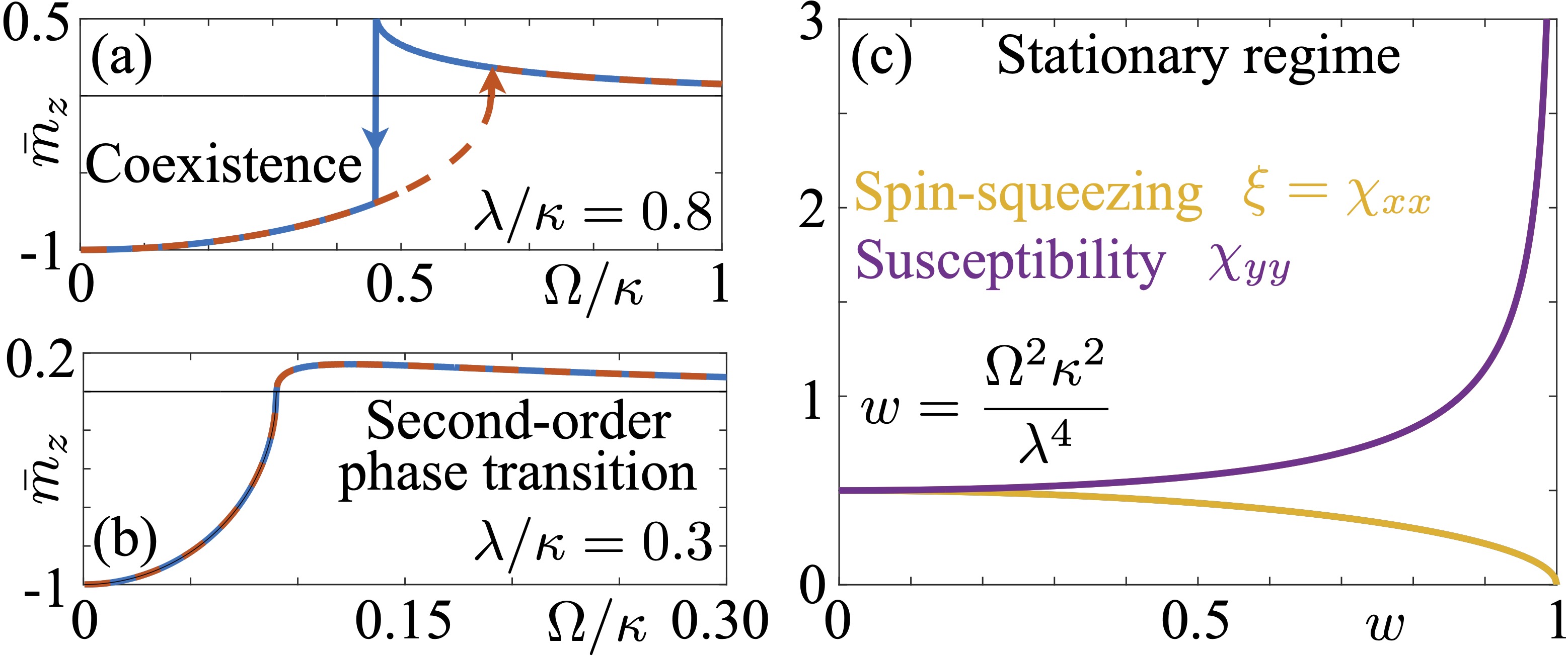
Figure 2: Coexistence and critical behavior. (a) Time-averaged $\bar{m}_{z}$ as a function of $\Omega$, for $\lambda/\kappa=0.8$ [upper dotted line in Fig. 1(b)]. The solid (dashed) curve is obtained by starting from the time-crystal (stationary) phase and moving “adiabatically” $\Omega$ towards the stationary (time-crystal) one. (b) Time-averaged $\bar{m}_{z}$ as a function of $\Omega$, for $\lambda/\kappa=0.3$ [lower dotted line in Fig. 1(b)]. Here, the phase transition is of second order [see also inset of Fig. 1(b)]. (c) Critical behavior of the spin-squeezing and of the susceptibility in the stationary regime, as a function of $(\Omega\kappa/\lambda^{2})^{2}$. The coordinates $x,y$ refers to the frame in which the $z$-axis is aligned with the direction of the vector identified by the stationary values in Eq. (4).

Phase diagram and bistability.— Having established the existence of a non-stationary regime, we now analyze in detail the nonequilibrium phase diagram of the system. We observe that, also within the parameter regime in which the stationary state of Eq. (4) is well-defined, the system can approach a limit cycle. This implies the existence of a region where the stationary phase [cf. Eq. (4)] and the time-crystal one coexist. Such bistable regimes usually occur for stationary phases (see, e.g., Refs. [114, 115]) and are characterized through a stability analysis. However, in our case one of the two asymptotic solutions is a limit cycle. As such, to fully explore the bistable region we take an approach which exploits the coexistence between the two phases. To treat the latter on an equal footing, we will focus on the time-averaged order-parameter $\bar{m}_{z}=\frac{1}{t}\int_{0}^{t}{\rm d}u\,m_{z}(u)$, which converges to the value in Eq. (4) within the stationary regime while it gives an average over the oscillations in the time-crystal phase.

When $\Omega>\lambda^{2}/\kappa$, the system can only be found in the time-crystal phase. The curve $\Omega=\lambda^{2}/\kappa$ thus provides one of the boundaries of the bistability region. To find the other boundary, i.e., the line separating the bistable regime from the stationary phase [cf. Fig. 1(b)], we probe coexistence behavior. The idea is as follows. We start at a point $(\Omega,\lambda)$ in parameter space, with $\Omega\gg\lambda$ where only the time-crystal phase is stable [cf. Fig. 1(b)]. We initialize the system in the state $\ket{\psi}$, with all atoms in the excited state $\ket{e}$ and the light field in the vacuum, and let it relax towards the asymptotic limit cycle. We then increase $\lambda$, in small discrete steps, in an adiabatically slow fashion, i.e., always giving the system sufficient time to accommodate into the new limit cycle. In this way, we can enter the bistable regime lying within the basin of attraction of the time-crystal phase. For sufficiently large $\lambda$, only the stationary phase is eventually stable. As shown in Fig. 1(b), this makes the second (upper) spinodal line emerge as the line where $\bar{m}_{z}$ jumps from positive values, attained in the time-crystal phase, to the negative ones given by Eq. (4). A similar sweep through the phase diagram can be done by fixing $\lambda$. This procedure also shows coexistence of the two phases as apparent from Fig. 2(a). The two spinodal lines meet at a tricritical point, highlighted in Fig. 1(b). Beyond this point, the phase transition does not switch to a crossover as it usually happens, but it rather changes nature and becomes a second-order one, see Fig. 2(b). Note that the curve in Fig. 2(b) displays a proper phase transition since i) the stationary value $m_{z}^{*}$ approaches the critical point with an infinite derivative [cf. Eq. (4)] and ii) as we calculate below and anticipate in Fig. 2(c), approaching the critical point from the stationary regime the system features a diverging susceptibility.

Dynamics of quantum fluctuations.— Average operators converge, in the thermodynamic limit, to multiples of the identity [116] and thus cannot carry information about correlations. The natural next step is thus to consider suitable susceptibility parameters. In analogy with classical central limit theorems, for the atoms we introduce the quantum fluctuation operators [117, 118, 119, 120, 121, 122, 49]

$$F_{r}^{N}=\frac{1}{\sqrt{2N}}\left(S_{r}-\langle S_{r}\rangle\right)\,,$$ (5)

whose variance, $\chi_{rr}=\langle F_{r}^{2}\rangle$, provides the fluctuations of the order parameter $m_{r}^{N}$, that is, its susceptibility. The operators in Eq. (5) retain a quantum character in the thermodynamic limit. To understand this, let us consider the state with all atoms in $\ket{e}$. The commutator $[F_{x}^{N},F_{y}^{N}]=im_{z}^{N}$ is proportional to an average operator and, thus, converges in the thermodynamic limit to the multiple of the identity $im_{z}$, with $m_{z}=1$, due to our choice of the state. This commutation relation identifies the limiting fluctuation operators, $q_{A}=\lim_{N\to\infty}F_{x}^{N}$ and $p_{A}=\lim_{N\to\infty}F_{y}^{N}$, as two (bosonic) quadrature operators such that $[q_{A},p_{A}]=i$. Together with these atom fluctuations, we consider the light-field fluctuation operators $q_{L}=q-\langle q\rangle$ and $p_{L}=p-\langle p\rangle$ [52]. The emergent two-mode bosonic description formed by the fluctuation operators $R=(q_{A},p_{A},q_{L},p_{L})^{T}$ can be used to analyze correlations between the atoms and the light field [52].

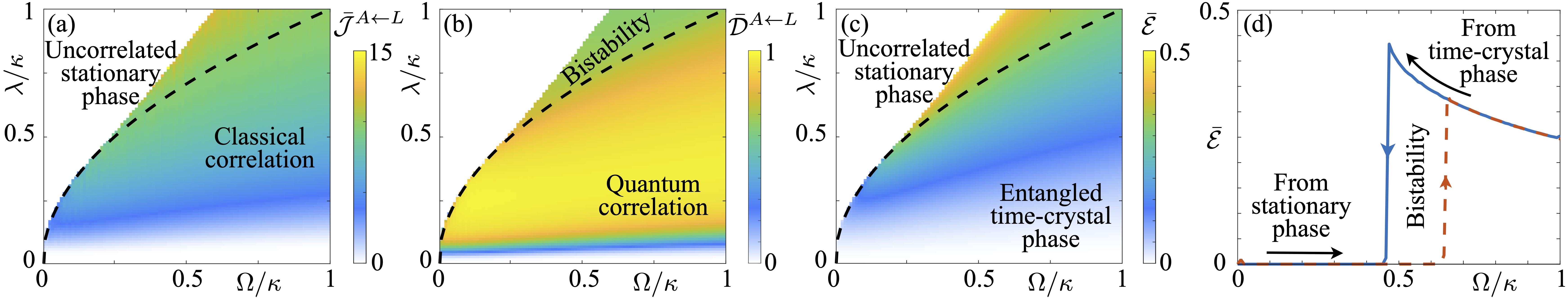
Figure 3: Quantum and classical correlations. (a) Time-averaged classical correlation $\bar{\mathcal{J}}^{A\leftarrow L}$, as a function of $\lambda$ and $\Omega$. For each value of $\Omega$, the data are obtained by initializing the system in state $\ket{\psi}$, evolving it with the smallest value of $\lambda$, and then adiabatically increasing the interaction parameter $\lambda$ in discrete steps up to the largest values. The evolution time for each value of $\lambda$ is $\kappa t=5000$ and coincides with the averaging window for the correlation measure. (b) Same as in panel (a) for the quantum discord $\bar{\mathcal{D}}^{A\leftarrow L}$. The latter shows that the time-crystal phase features quantum correlations. (c) Same as in panels (a) and (b) but for the logarithmic negativity quantifying the amount of entanglement between the atoms and the light field. (d) Coexistence of different bipartite entanglement behavior, as measured by the time-averaged logarithmic negativity $\bar{\mathcal{E}}$, for $\lambda/\kappa=0.8$ [cf. upper dotted line in Fig. 1(b)], and different values of $\Omega$ slowly varied in discrete steps both starting from the stationary phase and the time-crystal phase.

To this end, we introduce the covariance matrix $\Sigma_{uv}=\langle\{R_{u},R_{v}\}\rangle/2$ and derive its time evolution. Due to the dynamics of average operators, the commutation relation between the fluctuation operators associated with the atoms generically depends on time [49]. To “remove” this dependence, we move to the frame rotating with the time-evolving average operators. Here, we can derive the Lindblad generator for the dynamics of the two-mode bosonic system related to quantum fluctuations [109]. Dissipation solely affects the light field and is still described by the term in Eq. (2). The emergent two-mode Hamiltonian is

$$H_{A-L}(t)=\lambda\left[q_{A}p_{L}+m_{z}(t)q_{L}p_{A}\right]\,.$$ (6)

The latter is time-dependent as a consequence of the time-dependence of the average operator $m_{z}(t)$. This Hamiltonian can be decomposed into an excitation-exchange term, proportional to $1-m_{z}(t)$, and a two-mode squeezing term, proportional to $1+m_{z}(t)$ [109]. These contributions provide the only coupling between the atoms and the light field and, as we show below, can generate quantum correlations between the two subsystems. In contrast to the boundary time-crystal model [51], the dynamics of fluctuations is not fully dissipative due to the collective Hamiltonian in Eq. (1). Since the emergent dynamical generator is quadratic, quantum fluctuations remain Gaussian [123].

Quantum correlations and entanglement in the time-crystal regime.— From the time evolution of the covariance matrix $\Sigma$, we can calculate classical correlation, quantum discord [124, 125, 110, 111, 126], as well as bipartite (collective) entanglement between the atoms and the light field [112, 113], in the thermodynamic limit. Within the stationary phase, the asymptotic covariance matrix can be computed exactly as

$$\Sigma=\frac{1}{2}{\rm diag}(-m_{z}^{*},-(m_{z}^{*})^{-1},1,1)\,,$$ (7)

with $m_{z}^{*}$ as in Eq. (4). This expression shows that the light field (described by the operators $q_{L},p_{L}$) is in the vacuum state, while the collective atom operators $q_{A},p_{A}$ are in a squeezed state. Eq. (7) shows no correlations between the atoms and the light field in the stationary phase. Yet, the atoms display spin-squeezing, with a squeezing parameter, $\xi=|m_{z}^{*}|$, which diverges (to zero) on the spinodal line separating the bistable regime from the pure time-crystal phase. The divergence (to infinity) of $\Sigma_{22}\propto|1/m_{z}^{*}|$ is related to the divergence of the susceptibility close to the second-order phase transition [cf. Fig. 2(c)]. Since fluctuations are in the frame aligned with the direction of the state in Eq. (4), $\Sigma_{22}$, in the stationary regime and close to the phase transition line, is essentially the susceptibility of the order-parameter $m_{z}$.

We now turn to the time-crystal phase. Here, there is no significant spin-squeezing in the atom ensemble. Moreover, it can be shown that the determinant of the covariance matrix increases indefinitely with time, which indicates that the state of the system becomes more and more mixed. Nonetheless, in this regime the atoms and the light field are correlated. This can be seen, for instance, through the one-way classical correlation. This quantity is a measure of the maximal information about one of the two subsystems, let us say the atoms, that can be gained by performing measurements on the other subsystem, in our case the light field. This one-way classical correlation, denoted as $\mathcal{J}^{A\leftarrow L}$, is shown in Fig. 3(a) and demonstrates the existence of correlations in the time-crystal phase. Even more interestingly, also correlations of genuine quantum nature can be observed in this regime, as measured by the (one-way) quantum discord $\mathcal{D}^{A\leftarrow L}=\mathcal{I}-\mathcal{J}^{A\leftarrow L}$, with $\mathcal{I}$ being the mutual information between the atoms and light field. The quantum discord quantifies the amount of correlations which are not of classical nature. In Fig. 3(b), we show that in the time-crystal phase the quantum discord is non-zero throughout. (We report results for $\mathcal{J}^{A\rightarrow L},\mathcal{D}^{A\rightarrow L}$ in Ref. [109].) Remarkably, a fraction of these quantum correlations is related to bipartite entanglement between the atom ensemble and the light field, which can be quantified through the logarithmic negativity $\mathcal{E}$ shown in Fig. 3(c). Both classical and quantum correlations display coexistence behavior, as for instance shown in Fig. 3(d), due to the coexistence of the uncorrelated stationary phase and the correlated time-crystal.

Discussion.— The system we have investigated is related to the well-known boundary time-crystal model [19] through an adiabatic elimination of the light field [70, 71, 72, 60, 61]. For what concerns the atoms, it shows features which are similar to those of the boundary time-crystal. That is, we observe spin-squeezing in the stationary regime, and absence of quantum correlations among the atoms in the oscillatory phase [53, 36, 50, 51, 54, 55, 56]. However, explicitly considering the light field allowed us to uncover the existence of genuine quantum correlations in the time-crystal regime, even though the latter is characterized by a mixed state, established between atoms and light field. From a fundamental perspective our results demonstrate that time-crystal phases can display quantum correlations and are thus certainly not classical.

Finally, we note that the time-crystal phase appears to be related to lasing — since there is an inversion of population signalled by a positive magnetization $\bar{m}_{z}>0$ [13] — even though the model does not possess a $U(1)$ symmetry. This is due to the fact that the “pumping” is not incoherent but rather is implemented through external laser driving. However, the oscillations established are not harmonic [see inset of Fig. 1(b)] and, deep in the time-crystal phase, $|\Omega|\gg|\lambda|$, the time-averaged magnetization $\bar{m}_{z}$ tends to zero, i.e., there is no inversion of population [13].

Acknowledgments.— We are grateful for financing from the Baden-Württemberg Stiftung through Project No. BWST_ISF2019-23. We also acknowledge funding from the Deutsche Forschungsgemeinschaft (DFG, German Research Foundation) under Project No. 435696605 and through the Research Unit FOR 5413/1, Grant No. 465199066. This project has also received funding from the European Union’s Horizon Europe research and innovation program under Grant Agreement No. 101046968 (BRISQ), and from EPSRC under Grant No. EP/V031201/1. FC is indebted to the Baden-Württemberg Stiftung for the financial support of this research project by the Eliteprogramme for Postdocs.

SUPPLEMENTAL MATERIAL

Robert Mattes,¹ Igor Lesanovsky,^1,2 and Federico Carollo¹

¹Institut für Theoretische Physik, Universität Tübingen,
Auf der Morgenstelle 14, 72076 Tübingen, Germany
²School of Physics and Astronomy and Centre for the Mathematics
and Theoretical Physics of Quantum Non-Equilibrium Systems,
The University of Nottingham, Nottingham, NG7 2RD, United Kingdom

I. Equations for average operators and stationary state

Following the derivation put forward in Ref. [73], it is possible to show that, in the thermodynamic limit, the average operators evolve according to a set of nonlinear equations. These equations are the so-called mean-field equations and for the model considered they are given by

$$\dot{m}_{x}(t) =\sqrt{2}\lambda m_{q}(t)m_{z}(t)\,,$$

$$\ \dot{m}_{y}(t) =-2\Omega m_{z}(t)-\sqrt{2}\lambda m_{p}(t)m_{z}(t)\,,$$

$$\ \dot{m}_{z}(t) =2\Omega m_{y}(t)+\sqrt{2}\lambda m_{p}(t)m_{y}(t)-\sqrt{2}\lambda m_{q}(t)m_{x}(t)\,,$$

$$\ \dot{m}_{q}(t) =\frac{\lambda}{\sqrt{2}}m_{x}(t)-\frac{\kappa}{2}m_{q}(t)\,,$$

$$\ \dot{m}_{p}(t) =-\frac{\lambda}{\sqrt{2}}m_{y}(t)-\frac{\kappa}{2}m_{p}(t)\,.$$

For these equations, we have that $m_{x}^{2}+m_{y}^{2}+m_{z}^{2}$ is a conserved quantity, which we set equal to one. Moreover, it is possible to see that starting from a state with $m_{x}(0)=m_{q}(0)=0$ one has that $m_{x}(t)=m_{q}(t)=0$ for all later times $t>0$. With such an initial state the set of nonlinear differential equations reduces to

$$\begin{split}\dot{m}_{y}(t)&=-2\Omega m_{z}(t)-\sqrt{2}\lambda m_{p}(t)m_{z}(t)\,,\\ \ \dot{m}_{z}(t)&=2\Omega m_{y}(t)+\sqrt{2}\lambda m_{p}(t)m_{y}(t)\,,\\ \ \dot{m}_{p}(t)&=-\frac{\lambda}{\sqrt{2}}m_{y}(t)-\frac{\kappa}{2}m_{p}(t)\,.\end{split}$$ (S1)

By setting the derivatives to zero and using the constant of motion ($m_{x}^{2}+m_{y}^{2}+m_{z}^{2}=1$) the stationary solutions are given by

$$m_{y}^{*}=\frac{\Omega\kappa}{\lambda^{2}}\,, \,m_{z}^{*}=\pm\sqrt{1-\left(\frac{\Omega\kappa}{\lambda^{2}}\right)^{2}}\,, \,m_{p}^{*}=-\frac{\sqrt{2}\Omega}{\lambda}\,.$$ (S2)

The positive $m_{z}^{*}$ solution is unstable. This can be seen by analyzing the eigenvalues of the Jacobian matrix $J$, linearizing the above system of equations around the stationary solution. This matrix can be obtained by writing $m_{c}(t)\approx m_{c}^{*}+\delta m_{c}$, with the perturbation $\delta m_{c}$ small, and taking perturbations only up to first-order into account. The linearized Jacobian matrix takes the form

$$J=\left(\begin{array}[]{ccc}0&0&-\sqrt{2}\lambda m_{z}^{*}\\ 0&0&\sqrt{2}\lambda m_{y}^{*}\\ -\frac{\lambda}{\sqrt{2}}&0&-\frac{\kappa}{2}\end{array}\right)\,.$$

A stationary solution is stable if the real part of all the eigenvalues of the matrix $J$ is smaller or at most equal to zero. The eigenvalues $\mu_{i}$ of the matrix $J$ are given by

$$\mu_{1}=0 \mu_{2,3}=-\frac{\kappa}{4}\left(1\pm\sqrt{1+\frac{4\lambda^{2}m_{z}^{*}}{\left(\frac{\kappa}{2}\right)^{2}}}\right)\,.$$ and

This immediately shows that the stationary state with positive $m_{z}^{*}$ is unstable. The state with negative magnetization $m_{z}^{*}$ is instead stable, but it is only well-defined for $\Omega\kappa<\lambda^{2}$. Outside this regime, no stationary state exists within the sector identified by the choice of the conserved quantities.

II. Dynamics of quantum fluctuations

In this Section, we give details on the derivation of the evolution of the covariance matrix for fluctuation operators, as well as on the transformation to the frame which rotates solidly with the main direction of the atom average operators. We then explicitly derive the dynamical generator for quantum fluctuations in such rotating frame.

Time evolution of the covariance matrix of quantum fluctuations

The derivation of the time evolution of the covariance matrix for fluctuation operators follows closely the one presented in Ref. [52]. We start by introducing the vector of fluctuation operators $\tilde{R}^{N}=(F^{N}_{x},F^{N}_{y},F^{N}_{z},q_{L},p_{L})^{T}$ in the time-independent frame. The covariance matrix of these fluctuation operators can be written as $\tilde{\Sigma}=\underset{N\to\infty}{\lim}\left(K^{N}+(K^{N})^{T}\right)/2$, where we have defined $K_{uv}^{N}=\left\langle\tilde{R}_{u}^{N}\tilde{R}_{v}^{N}\right\rangle$. Here, the expectation $\langle\cdot\rangle$ denotes expectation with respect to the state at time $t$.

We now consider the time evolution of this correlation function $K_{uv}^{N}$. First, we note that

$$\dot{F^{N}_{u}}=-\frac{1}{\sqrt{2N}}\dot{\langle S_{u}\rangle}\,,\mbox{ for }u=x,y,z\,,$$

as well as $\dot{q_{L}}=-\dot{\langle q\rangle}$ and $\dot{p_{L}}=-\dot{\langle p\rangle}$, and that $\langle\tilde{R}_{u}^{N}\rangle=0$. Taking the time derivative of $K^{N}_{uv}$ then leads to

$$\dot{K}_{uv}^{N}=\left\langle i\left[H,\tilde{R}_{u}^{N}\right]\tilde{R}_{v}^{N}\right\rangle+\left\langle i\tilde{R}_{u}^{N}\left[H,\tilde{R}_{v}^{N}\right]\right\rangle+\left\langle\mathcal{L}^{*}\left[\tilde{R}_{u}^{N}\tilde{R}_{v}^{N}\right]\right\rangle\,,$$

where $\mathcal{L}^{*}$ is the dissipator in the Heisenberg picture, i.e., the map dual to $\mathcal{L}$. To proceed, we compute the commutators in the above equations which can then be rewritten in terms of fluctuation operators exploiting again that $\langle\tilde{R}_{u}^{N}\rangle=0$. A similar calculation also applies to the dissipative part in the above equation. As in Ref. [52], this gives rise to products of fluctuation operators and average operators. Making use of the fact that, in the thermodynamic limit, $\underset{N\to\infty}{\lim}\left\langle\tilde{R}_{r}^{N}m_{u}^{N}\tilde{R}_{v}^{N}\right\rangle=m_{u}(t)\left\langle\tilde{R}_{r}\tilde{R}_{v}\right\rangle$, and recalling the relation between $K^{N}$ and the covariance matrix, we find that

$$\dot{\tilde{\Sigma}}(t)=\tilde{W}(t)\tilde{\Sigma}(t)+\tilde{\Sigma}(t)\tilde{W}^{T}(t)+\tilde{S}(t){A}\tilde{S}^{T}(t)\,, \tilde{W}(t)=\tilde{P}(t)+\tilde{S}(t)B\,.$$ with

Here, we have defined the symplectic matrix

$$\tilde{S}(t)=\left(\begin{array}[]{ccccc}0&m_{z}(t)&-m_{y}(t)&0&0\\ -m_{z}(t)&0&m_{x}(t)&0&0\\ m_{y}(t)&-m_{x}(t)&0&0&0\\ 0&0&0&0&1\\ 0&0&0&-1&0\\ \end{array}\right)\,,$$

encoding the commutation relation between fluctuation operators. We further have that

$$C=\frac{\kappa}{2}\left(\begin{array}[]{ccccc}0&0&0&0&0\\ 0&0&0&0&0\\ 0&0&0&0&0\\ 0&0&0&1&i\\ 0&0&0&-i&1\end{array}\right)\,,$$

through which we can define $A=(C+C^{T})/2$ and $B=(C-C^{T})/(2i)$, and

$$\tilde{P}(t)=\left(\begin{array}[]{ccccc}0&0&\sqrt{2}\lambda m_{q}(t)&\lambda m_{z}(t)&0\\ 0&0&-2\Omega-\sqrt{2}\lambda m_{p}(t)&0&-\lambda m_{z}(t)\\ -\sqrt{2}\lambda m_{q}(t)&2\Omega+\sqrt{2}\lambda m_{p}(t)&0&-\lambda m_{x}(t)&\lambda m_{y}(t)\\ \lambda&0&0&0&0\\ 0&-\lambda&0&0&0\end{array}\right)\,.$$

The evolution for the case considered in the main text is obtained by setting $m_{x}=m_{q}=0$.

Covariance matrix in the rotating frame

We now focus on the case in which the system in initialized in the state with all atoms in $\ket{e}$ and the light field in the vacuum. This gives $m_{x}(t)=m_{q}(t)=0$ and $m_{y}^{2}(t)+m_{z}^{2}(t)=1$. This is the initial state considered for producing the plots in the main text. Our task is now to find the time evolution of the covariance matrix in the frame which rotates solidly with the direction identified by the average operators. To rotate the reference frame of the atom operators back to the initial one, we need to find the rotation matrix which maps the instantaneous vector of the average operators $m=[0,m_{y}(t),m_{z}(t),m_{q}(t),0]^{T}$ into the one $m=[0,0,1,m_{q}(t),0]^{T}$. Exploiting the conservation law $m_{y}^{2}(t)+m_{z}^{2}(t)=1$, this matrix can be found to be the matrix

$$U(t)=\left(\begin{array}[]{ccccc}1&0&0&0&0\\ 0&m_{z}(t)&-m_{y}(t)&0&0\\ 0&m_{y}(t)&m_{z}(t)&0&0\\ 0&0&0&1&0\\ 0&0&0&0&1\\ \end{array}\right)\,.$$

Under this transformation, the symplectic matrix becomes

$$S=U(t)\tilde{S}(t)U^{T}(t)=\left(\begin{array}[]{ccccc}0&1&0&0&0\\ -1&0&0&0&0\\ 0&0&0&0&0\\ 0&0&0&0&1\\ 0&0&0&-1&0\\ \end{array}\right)\,.$$

The time evolution of the covariance matrix in the rotating frame can be calculated by taking the derivative of $\hat{\Sigma}=U(t)\tilde{\Sigma}(t)U^{T}(t)$, which gives

$$\dot{{\hat{\Sigma}}}(t)=Q(t){\hat{\Sigma}}(t)+{\hat{\Sigma}}(t)Q^{T}(t)+SAS^{T}\,, Q(t)=\left(\begin{array}[]{ccccc}0&0&0&\lambda m_{z}(t)&0\\ 0&0&0&0&-\lambda\\ 0&0&0&0&0\\ \lambda&0&0&-\frac{\kappa}{2}&0\\ 0&-\lambda m_{z}(t)&-\lambda m_{y}(t)&0&-\frac{\kappa}{2}\end{array}\right)\,.$$ where (S8)

For the considered initial state, the covariance matrix is given by the diagonal matrix $\hat{\Sigma}(0)=1/2\,{\rm diag}(1,1,0,1,1)$. Starting from this covariance matrix, it is possible to see that the third row and the third column of the covariance matrix are not coupled with the remainder of the matrix. We thus define ${\Sigma}$ to be the covariance matrix of the fluctuation operator $q_{A}$ (which is the limiting operator of the fluctuation $F_{x}^{N}$ in the rotating frame), $p_{A}$ (which is the limiting operator of the fluctuation $F_{y}^{N}$ in the rotating frame) coupled to the fluctuations $q_{L}$,$p_{L}$ (see also main text).

For such a matrix, the time evolution is given by the equation

$$\dot{\Sigma}(t)=X(t)\Sigma(t)+\Sigma(t)X^{T}(t)+sas^{T}\,,$$ (S9)

where $X,s,a$ are the $4\times 4$ matrices obtained by removing the third row and third column in $Q,S,A$ respectively.

Dynamical generator for the quantum fluctuation dynamics in the rotating frame

We now want to find the generator for the dynamics of the two-mode bosonic system described by the vector of bosonic operators $R=(q_{A},p_{A},q_{L},p_{L})^{T}$. As done in Ref. [51], to this end we consider a time-dependent Lindblad generator on bosonic operator of the form

$$\mathcal{W}^{*}_{A-L}(t)[O]=i[H_{A-L}(t),O]+\mathcal{L}^{*}[O]\,,$$

with an ansatz for the Hamiltonian given by

$$H_{A-L}(t)=\sum_{i,j=1}^{4}h_{ij}(t)R_{i}R_{j}\,.$$

The dissipative part of the generator is equal to the one of the original system, since the fluctuation of the light field are just the rescaled original operators. Using the generator $\mathcal{W}_{A-L}^{*}(t)$ to calculate the time evolution of the covariance matrix one finds

$$\dot{\Sigma}(t)=[2sh(t)+sb]\Sigma(t)+\Sigma(t)[2sh(t)+sb]^{T}+sas^{T}\,.$$

Here, we have that the $4\times 4$ matrix $b$ is obtained by removing the third row and the third column from the matrix $B$ introduced above. Comparing the above equation with Eq. (S9) gives that the generator correctly captures the dynamics of the covariance matrix if the relation

$$2sh(t)=\begin{pmatrix}0&0&\lambda m_{z}(t)&0\\ 0&0&0&-\lambda\\ \lambda&0&0&0\\ 0&-\lambda m_{z}(t)&0&0\end{pmatrix}\,$$

is satisfied. Exploiting that $s^{2}=-\mathbb{I}$, we can invert the relation to find

$$h(t)=\frac{\lambda}{2}\begin{pmatrix}0&0&0&1\\ 0&0&m_{z}(t)&0\\ 0&m_{z}(t)&0&0\\ 1&0&0&0\end{pmatrix}\,,$$

which provides the Hamiltonian reported in the main text.

To show that the latter can be decomposed into a excitation-exchange term and a two-mode squeezing contribution, we represent the fluctuation operators $q_{A},p_{A},q_{L},p_{L}$ in terms of bosonic creation and annihilation operators. Due to the definition of the original quadrature operators of the light field, we write

$$q_{L}=\frac{i}{\sqrt{2}}\left(\phi_{L}-\phi_{L}^{\dagger}\right)\,,\qquad p_{L}=\frac{1}{\sqrt{2}}(\phi_{L}+\phi_{L}^{\dagger})\,.$$ (S10)

For the fluctuations of the atoms, we instead recall that $q_{A}$ is the limit of $F_{x}^{N}$ and $p_{A}$ the one of $F_{y}^{N}$ and, in order to associated the annihilation operator with $S_{-}$, we write

$$q_{A}=\frac{1}{\sqrt{2}}\left(\phi_{A}+\phi_{A}^{\dagger}\right)\,,\qquad p_{A}=\frac{i}{\sqrt{2}}\left(\phi_{A}^{\dagger}-\phi_{A}\right)\,.$$

Substituting these definitions into the Hamiltonian reported in the main text, we find

$$H_{A-L}(t)=\frac{\lambda}{2}\left[\left(\phi_{A}\phi_{L}+\phi_{A}^{\dagger}\phi_{L}^{\dagger}\right)\left[1+m_{z}(t)\right]+\left(\phi_{L}^{\dagger}\phi_{A}+\phi_{A}^{\dagger}\phi_{L}\right)\left[1-m_{z}(t)\right]\right]\,.$$

III. Quantum and classical correlations

In this Section, we describe how to calculate the correlation measures that we analyze in our work and we further present additional results on these. For details on the derivation of these measures, we refer to Refs. [110, 111, 112, 113].

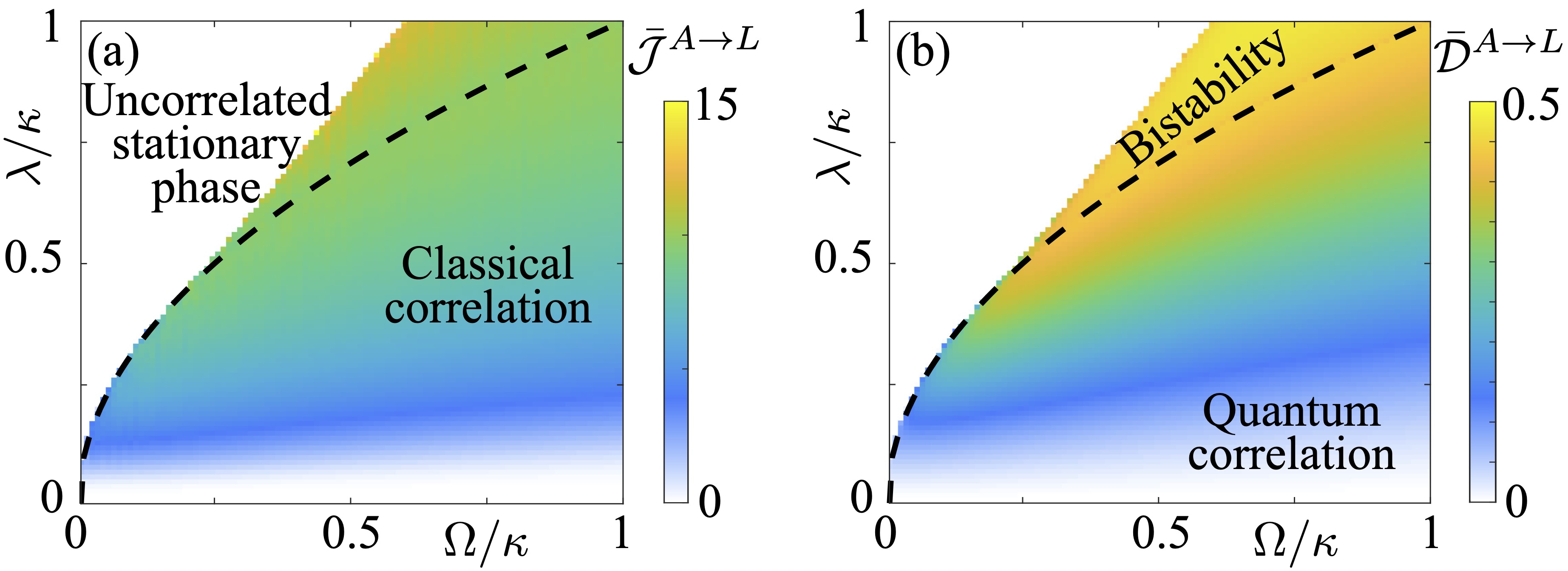
Figure S1: Additional results on quantum and classical correlations. (a) Time-averaged classical correlation $\bar{\mathcal{J}}^{A\rightarrow L}$, as a function of $\lambda$ and $\Omega$. For each value of $\Omega$, the data are obtained by initializing the system in state $\ket{\psi}$, evolving it with the smallest value of $\lambda$, and then adiabatically increasing the interaction parameter $\lambda$ in discrete steps up to the largest values. The evolution time for each value of $\lambda$ is $\kappa t=5000$ and coincides with the averaging window for the correlation measure. (b) Same as in panel (a) for the quantum discord $\bar{\mathcal{D}}^{A\rightarrow L}$. The latter shows that the time-crystal phase features quantum correlations.

Given the two-mode covariance matrix $\Sigma(t)$, we now show how to compute measures for the classical correlation, for the quantum discord, and for the logarithmic negativity. To start, we identify the relevant $2\times 2$ minors of $\Sigma$ as the matrices $\alpha$, $\beta$ and $\gamma$, such that

$$2\Sigma(t)=\begin{pmatrix}\alpha&\gamma\\ \gamma&\beta\,.\end{pmatrix}$$

Here, the matrix $\alpha$ contains the variances of the atom fluctuations, $\beta$ those of the light-field fluctuations, while $\gamma$ contains the covariances between the atoms and the light field. We now define the quantities

$$c_{\alpha}={\rm det}(\alpha)\,,\qquad c_{\beta}={\rm det}(\beta)\,,\qquad c_{\gamma}={\rm det}(\gamma)\,,\qquad c_{\delta}={\rm det}(2\Sigma)\,$$

as well as the function

$$f(x)=\left(\frac{x+1}{2}\right)\log\left(\frac{x+1}{2}\right)-\left(\frac{x-1}{2}\right)\log\left(\frac{x-1}{2}\right)\,.$$

For a two-mode Gaussian state an expression for the one-way classical correlation, quantifying the information on the first mode obtained by measurements performed on the second mode, is given by

$$\mathcal{J}^{A\leftarrow L}=f(\sqrt{c_{\alpha}})-f(\sqrt{E_{\mathrm{min}}})\,,$$ (S11)

while the quantum discord is

$$\mathcal{D}^{A\leftarrow L}=f(\sqrt{c_{\beta}})-f(\nu_{-})-f(\nu_{+})+f(\sqrt{E_{\mathrm{min}}})\,,$$ (S12)

where $E_{\mathrm{min}}$ is defined as

$$E_{\mathrm{min}}=\left\{\begin{array}[]{cc}\frac{2c_{\gamma}^{2}+(c_{\beta}-1)(c_{\delta}-c_{\alpha})+2|c_{\gamma}|\sqrt{c_{\gamma}^{2}+(c_{\beta}-1)(c_{\delta}-c_{\alpha})}}{(c_{\beta}-1)^{2}}&\textrm{for}\,(c_{\delta}-c_{\alpha}c_{\beta})^{2}\leq(1+c_{\beta})c_{\gamma}^{2}(c_{\alpha}+c_{\delta})\,,\\ \frac{c_{\alpha}c_{\beta}-c_{\gamma}^{2}+c_{\delta}-\sqrt{c_{\gamma}^{4}+(c_{\delta}-c_{\alpha}c_{\beta})^{2}-2c_{\gamma}^{2}(c_{\alpha}c_{\beta}+c_{\delta})}}{2c_{\beta}}&\textrm{otherwise}\,.\end{array}\right.$$

The quantities $\nu_{-}$ and $\nu_{+}$ are the symplectic eigenvalues of the matrix $2\Sigma$, with $\nu_{-}<\nu_{+}$. These are found as the positive eigenvalues of the matrix $2is\Sigma$. To compute the correlations $\mathcal{J}^{A\rightarrow L}$ and $\mathcal{D}^{A\rightarrow L}$, quantifying the information about the light field that can be obtained from a measurement on the atoms, one can exploit the same definitions as above but exchanging the roles of $\alpha$ and $\beta$ in all of the above relations.

In order to quantify the amount of bipartite entanglement between the atoms and the light field, we compute the logarithmic negativity. This is defined as

$$\mathcal{E}=\text{max}\left(0,-\log\left(\tilde{\nu}_{-}\right)\right)\,,$$

where $\tilde{\nu}_{-}$ is the smallest symplectic eigenvalue of the partially transposed covariance $\Sigma^{PT}=\Lambda\Sigma\Lambda$, where $\Lambda={\rm diag}(1,1,1,-1)$. The latter is computed as the smallest positive eigenvalues of the matrix $2is\Sigma^{PT}$.

References

- Dicke [1954] R. H. Dicke, Coherence in Spontaneous Radiation Processes, Phys. Rev. 93, 99 (1954).
- Hepp and Lieb [1973a] K. Hepp and E. H. Lieb, On the superradiant phase transition for molecules in a quantized radiation field: the Dicke maser model, Ann. Phys. 76, 360 (1973a).
- Hepp and Lieb [1973b] K. Hepp and E. H. Lieb, Equilibrium statistical mechanics of matter interacting with the quantized radiation field, Phys. Rev. A 8, 2517 (1973b).
- Wang and Hioe [1973] Y. K. Wang and F. T. Hioe, Phase Transition in the Dicke Model of Superradiance, Phys. Rev. A 7, 831 (1973).
- Hioe [1973] F. T. Hioe, Phase Transitions in Some Generalized Dicke Models of Superradiance, Phys. Rev. A 8, 1440 (1973).
- Carmichael et al. [1973] H. Carmichael, C. Gardiner, and D. Walls, Higher order corrections to the Dicke superradiant phase transition, Phys. Lett. A 46, 47 (1973).
- Gross and Haroche [1982] M. Gross and S. Haroche, Superradiance: An essay on the theory of collective spontaneous emission, Phys. Rep. 93, 301 (1982).
- Emary and Brandes [2003a] C. Emary and T. Brandes, Chaos and the quantum phase transition in the Dicke model, Phys. Rev. E 67, 066203 (2003a).
- Emary and Brandes [2003b] C. Emary and T. Brandes, Quantum Chaos Triggered by Precursors of a Quantum Phase Transition: The Dicke Model, Phys. Rev. Lett. 90, 044101 (2003b).
- Lambert et al. [2005] N. Lambert, C. Emary, and T. Brandes, Entanglement and entropy in a spin-boson quantum phase transition, Phys. Rev. A 71, 053804 (2005).
- Bastidas et al. [2012] V. M. Bastidas, C. Emary, B. Regler, and T. Brandes, Nonequilibrium Quantum Phase Transitions in the Dicke Model, Phys. Rev. Lett. 108, 043003 (2012).
- Keeling et al. [2010] J. Keeling, M. J. Bhaseen, and B. D. Simons, Collective Dynamics of Bose-Einstein Condensates in Optical Cavities, Phys. Rev. Lett. 105, 043001 (2010).
- Kirton et al. [2019] P. Kirton, M. M. Roses, J. Keeling, and E. G. Dalla Torre, Introduction to the Dicke Model: From Equilibrium to Nonequilibrium, and Vice Versa, Adv. Quantum Technol. 2, 1800043 (2019).
- Zhiqiang et al. [2017] Z. Zhiqiang, C. H. Lee, R. Kumar, K. J. Arnold, S. J. Masson, A. S. Parkins, and M. D. Barrett, Nonequilibrium phase transition in a spin-1 Dicke model, Optica 4, 424 (2017).
- Zhiqiang et al. [2018] Z. Zhiqiang, C. H. Lee, R. Kumar, K. J. Arnold, S. J. Masson, A. L. Grimsmo, A. S. Parkins, and M. D. Barrett, Dicke-model simulation via cavity-assisted Raman transitions, Phys. Rev. A 97, 043858 (2018).
- Stitely et al. [2020] K. C. Stitely, S. J. Masson, A. Giraldo, B. Krauskopf, and S. Parkins, Superradiant switching, quantum hysteresis, and oscillations in a generalized Dicke model, Phys. Rev. A 102, 063702 (2020).
- Shchadilova et al. [2020] Y. Shchadilova, M. M. Roses, E. G. Dalla Torre, M. D. Lukin, and E. Demler, Fermionic formalism for driven-dissipative multilevel systems, Phys. Rev. A 101, 013817 (2020).
- Stitely et al. [2022] K. C. Stitely, A. Giraldo, B. Krauskopf, and S. Parkins, Lasing and counter-lasing phase transitions in a cavity-QED system, Phys. Rev. Res. 4, 023101 (2022).
- Iemini et al. [2018] F. Iemini, A. Russomanno, J. Keeling, M. Schirò, M. Dalmonte, and R. Fazio, Boundary time crystals, Phys. Rev. Lett. 121, 035301 (2018).
- Buča et al. [2019] B. Buča, J. Tindall, and D. Jaksch, Non-stationary coherent quantum many-body dynamics through dissipation, Nat. Commun. 10, 1730 (2019).
- Buča and Jaksch [2019] B. Buča and D. Jaksch, Dissipation Induced Nonstationarity in a Quantum Gas, Phys. Rev. Lett. 123, 260401 (2019).
- Chiacchio and Nunnenkamp [2019] E. I. R. Chiacchio and A. Nunnenkamp, Dissipation-Induced Instabilities of a Spinor Bose-Einstein Condensate Inside an Optical Cavity, Phys. Rev. Lett. 122, 193605 (2019).
- Booker et al. [2020] C. Booker, B. Buča, and D. Jaksch, Non-stationarity and dissipative time crystals: spectral properties and finite-size effects, New J. Phys. 22, 085007 (2020).
- Wilczek [2012] F. Wilczek, Quantum time crystals, Phys. Rev. Lett. 109, 160401 (2012).
- Shapere and Wilczek [2012] A. Shapere and F. Wilczek, Classical Time Crystals, Phys. Rev. Lett. 109, 160402 (2012).
- Bruno [2013] P. Bruno, Impossibility of Spontaneously Rotating Time Crystals: A No-Go Theorem, Phys. Rev. Lett. 111, 070402 (2013).
- Watanabe and Oshikawa [2015] H. Watanabe and M. Oshikawa, Absence of Quantum Time Crystals, Phys. Rev. Lett. 114, 251603 (2015).
- Sacha [2015] K. Sacha, Modeling spontaneous breaking of time-translation symmetry, Phys. Rev. A 91, 033617 (2015).
- Khemani et al. [2016] V. Khemani, A. Lazarides, R. Moessner, and S. L. Sondhi, Phase Structure of Driven Quantum Systems, Phys. Rev. Lett. 116, 250401 (2016).
- Else et al. [2016] D. V. Else, B. Bauer, and C. Nayak, Floquet time crystals, Phys. Rev. Lett. 117, 090402 (2016).
- Yao et al. [2017] N. Y. Yao, A. C. Potter, I.-D. Potirniche, and A. Vishwanath, Discrete time crystals: Rigidity, criticality, and realizations, Phys. Rev. Lett. 118, 030401 (2017).
- Sacha and Zakrzewski [2017] K. Sacha and J. Zakrzewski, Time crystals: a review, Rep. Prog. Phys. 81, 016401 (2017).
- Gambetta et al. [2019] F. Gambetta, F. Carollo, M. Marcuzzi, J. Garrahan, and I. Lesanovsky, Discrete time crystals in the absence of manifest symmetries or disorder in open quantum systems, Phys. Rev. Lett. 122, 015701 (2019).
- Else et al. [2020] D. V. Else, C. Monroe, C. Nayak, and N. Y. Yao, Discrete time crystals, Annu. Rev. Condens. Matter Phys. 11, 467 (2020).
- Taheri et al. [2022] H. Taheri, A. B. Matsko, L. Maleki, and K. Sacha, All-optical dissipative discrete time crystals, Nat. Commun. 13, 848 (2022).
- Sánchez Muñoz et al. [2019] C. Sánchez Muñoz, B. Buča, J. Tindall, A. González-Tudela, D. Jaksch, and D. Porras, Symmetries and conservation laws in quantum trajectories: Dissipative freezing, Phys. Rev. A 100, 042113 (2019).
- Piccitto et al. [2021] G. Piccitto, M. Wauters, F. Nori, and N. Shammah, Symmetries and conserved quantities of boundary time crystals in generalized spin models, Phys. Rev. B 104, 014307 (2021).
- Prazeres et al. [2021] L. F. d. Prazeres, L. d. S. Souza, and F. Iemini, Boundary time crystals in collective -level systems, Phys. Rev. B 103, 184308 (2021).
- Passarelli et al. [2022] G. Passarelli, P. Lucignano, R. Fazio, and A. Russomanno, Dissipative time crystals with long-range lindbladians, Phys. Rev. B 106, 224308 (2022).
- Ferioli et al. [2022] G. Ferioli, A. Glicenstein, I. Ferrier-Barbut, and A. Browaeys, Observation of a non-equilibrium superradiant phase transition in free space, arXiv:2207.10361 (2022).
- Chase and Geremia [2008] B. A. Chase and J. M. Geremia, Collective processes of an ensemble of spin-1/2 particles, Phys. Rev. A 78, 052101 (2008).
- Baragiola et al. [2010] B. Q. Baragiola, B. A. Chase, and J. Geremia, Collective uncertainty in partially polarized and partially decohered spin-1/2 systems, Phys. Rev. A 81, 032104 (2010).
- Kirton and Keeling [2017] P. Kirton and J. Keeling, Suppressing and Restoring the Dicke Superradiance Transition by Dephasing and Decay, Phys. Rev. Lett. 118, 123602 (2017).
- Kirton and Keeling [2018] P. Kirton and J. Keeling, Superradiant and lasing states in driven-dissipative Dicke models, New J. Phys. 20, 015009 (2018).
- Shammah et al. [2018] N. Shammah, S. Ahmed, N. Lambert, S. De Liberato, and F. Nori, Open quantum systems with local and collective incoherent processes: Efficient numerical simulations using permutational invariance, Phys. Rev. A 98, 063815 (2018).
- Huybrechts et al. [2020] D. Huybrechts, F. Minganti, F. Nori, M. Wouters, and N. Shammah, Validity of mean-field theory in a dissipative critical system: Liouvillian gap, -symmetric antigap, and permutational symmetry in the model, Phys. Rev. B 101, 214302 (2020).
- Carmichael [1980] H. J. Carmichael, Analytical and numerical results for the steady state in cooperative resonance fluorescence, J. Phys. B: Atom. Mol. Phys. 13, 3551 (1980).
- Alicki and Messer [1983] R. Alicki and J. Messer, Nonlinear quantum dynamical semigroups for many-body open systems, J. Stat. Phys. 32, 299 (1983).
- Benatti et al. [2018] F. Benatti, F. Carollo, R. Floreanini, and H. Narnhofer, Quantum spin chain dissipative mean-field dynamics, J. Phys. A 51, 325001 (2018).
- Buonaiuto et al. [2021] G. Buonaiuto, F. Carollo, B. Olmos, and I. Lesanovsky, Dynamical Phases and Quantum Correlations in an Emitter-Waveguide System with Feedback, Phys. Rev. Lett. 127, 133601 (2021).
- Carollo and Lesanovsky [2022] F. Carollo and I. Lesanovsky, Exact solution of a boundary time-crystal phase transition: time-translation symmetry breaking and non-Markovian dynamics of correlations, Phys. Rev. A 105, L040202 (2022).
- Boneberg et al. [2022] M. Boneberg, I. Lesanovsky, and F. Carollo, Quantum fluctuations and correlations in open quantum Dicke models, Phys. Rev. A 106, 012212 (2022).
- Hannukainen and Larson [2018] J. Hannukainen and J. Larson, Dissipation-driven quantum phase transitions and symmetry breaking, Phys. Rev. A 98, 042113 (2018).
- Lourenço et al. [2022] A. C. Lourenço, L. F. d. Prazeres, T. O. Maciel, F. Iemini, and E. I. Duzzioni, Genuine multipartite correlations in a boundary time crystal, Phys. Rev. B 105, 134422 (2022).
- Montenegro et al. [2023] V. Montenegro, M. G. Genoni, A. Bayat, and M. G. A. Paris, Quantum-Enhanced Boundary Time Crystal Sensors, arXiv:2301.02103 (2023).
- Pavlov et al. [2023] V. P. Pavlov, D. Porras, and P. A. Ivanov, Quantum metrology with critical driven-dissipative collective spin system, arXiv:2302.05216 (2023).
- Cabot et al. [2022] A. Cabot, F. Carollo, and I. Lesanovsky, Metastable discrete time-crystal resonances in a dissipative central spin system, Phys. Rev. B 106, 134311 (2022).
- Tavis and Cummings [1967] M. Tavis and F. Cummings, The exact solution of N two level systems interacting with a single mode, quantized radiation field, Phys. Lett. A 25, 714 (1967).
- Tavis and Cummings [1969] M. Tavis and F. W. Cummings, Approximate Solutions for an -Molecule-Radiation-Field Hamiltonian, Phys. Rev. 188, 692 (1969).
- Carollo et al. [2020] F. Carollo, K. Brandner, and I. Lesanovsky, Nonequilibrium Many-Body Quantum Engine Driven by Time-Translation Symmetry Breaking, Phys. Rev. Lett. 125, 240602 (2020).
- Paulino et al. [2022] P. J. Paulino, I. Lesanovsky, and F. Carollo, Nonequilibrium thermodynamics and power generation in open quantum optomechanical systems, arXiv:2212.10194 (2022).
- Ritsch et al. [2013] H. Ritsch, P. Domokos, F. Brennecke, and T. Esslinger, Cold atoms in cavity-generated dynamical optical potentials, Rev. Mod. Phys. 85, 553 (2013).
- Feng et al. [2015] M. Feng, Y. P. Zhong, T. Liu, L. L. Yan, W. L. Yang, J. Twamley, and H. Wang, Exploring the quantum critical behaviour in a driven Tavis–Cummings circuit, Nat. Commun. 6, 7111 (2015).
- Norcia et al. [2016] M. A. Norcia, M. N. Winchester, J. R. K. Cline, and J. K. Thompson, Superradiance on the millihertz linewidth strontium clock transition, Sci. Adv. 2, e1601231 (2016).
- Rose et al. [2017] B. C. Rose, A. M. Tyryshkin, H. Riemann, N. V. Abrosimov, P. Becker, H.-J. Pohl, M. L. W. Thewalt, K. M. Itoh, and S. A. Lyon, Coherent Rabi Dynamics of a Superradiant Spin Ensemble in a Microwave Cavity, Phys. Rev. X 7, 031002 (2017).
- Norcia et al. [2018] M. A. Norcia, R. J. Lewis-Swan, J. R. K. Cline, B. Zhu, A. M. Rey, and J. K. Thompson, Cavity-mediated collective spin-exchange interactions in a strontium superradiant laser, Science 361, 259 (2018).
- Dogra et al. [2019] N. Dogra, M. Landini, K. Kroeger, L. Hruby, T. Donner, and T. Esslinger, Dissipation-induced structural instability and chiral dynamics in a quantum gas, Science 366, 1496 (2019).
- Schäffer et al. [2020] S. A. Schäffer, M. Tang, M. R. Henriksen, A. A. Jørgensen, B. T. R. Christensen, and J. W. Thomsen, Lasing on a narrow transition in a cold thermal strontium ensemble, Phys. Rev. A 101, 013819 (2020).
- Mivehvar et al. [2021] F. Mivehvar, F. Piazza, T. Donner, and H. Ritsch, Cavity QED with quantum gases: new paradigms in many-body physics, Adv. Phys. 70, 1 (2021).
- Agarwal et al. [1997] G. S. Agarwal, R. R. Puri, and R. P. Singh, Atomic Schrödinger cat states, Phys. Rev. A 56, 2249 (1997).
- Gopalakrishnan et al. [2011] S. Gopalakrishnan, B. L. Lev, and P. M. Goldbart, Frustration and Glassiness in Spin Models with Cavity-Mediated Interactions, Phys. Rev. Lett. 107, 277201 (2011).
- Damanet et al. [2019] F. Damanet, A. J. Daley, and J. Keeling, Atom-only descriptions of the driven-dissipative Dicke model, Phys. Rev. A 99, 033845 (2019).
- Carollo and Lesanovsky [2021] F. Carollo and I. Lesanovsky, Exactness of Mean-Field Equations for Open Dicke Models with an Application to Pattern Retrieval Dynamics, Phys. Rev. Lett. 126, 230601 (2021).
- Lindblad [1976] G. Lindblad, On the generators of quantum dynamical semigroups, Commun. Math. Phys. 48, 119 (1976).
- Gorini et al. [1976] V. Gorini, A. Kossakowski, and E. C. G. Sudarshan, Completely positive dynamical semigroups of N‐level systems, J. Math. Phys. 17, 821 (1976).
- Bogoliubov et al. [1996] N. M. Bogoliubov, R. K. Bullough, and J. Timonen, Exact solution of generalized Tavis - Cummings models in quantum optics, J. Phys. A Math. Gen. 29, 6305 (1996).
- López et al. [2007] C. E. López, F. Lastra, G. Romero, and J. C. Retamal, Concurrence in the inhomogeneous Tavis-Cummings model, J. Phys.: Conf. Ser. 84, 012013 (2007).
- Wood et al. [2014] C. J. Wood, T. W. Borneman, and D. G. Cory, Cavity Cooling of an Ensemble Spin System, Phys. Rev. Lett. 112, 050501 (2014).
- Genway et al. [2014] S. Genway, W. Li, C. Ates, B. P. Lanyon, and I. Lesanovsky, Generalized Dicke Nonequilibrium Dynamics in Trapped Ions, Phys. Rev. Lett. 112, 023603 (2014).
- Lamata [2017] L. Lamata, Digital-analog quantum simulation of generalized Dicke models with superconducting circuits, Sci. Rep. 7, 43768 (2017).
- Trivedi et al. [2019] R. Trivedi, M. Radulaski, K. A. Fischer, S. Fan, and J. Vučković, Photon Blockade in Weakly Driven Cavity Quantum Electrodynamics Systems with Many Emitters, Phys. Rev. Lett. 122, 243602 (2019).
- Andolina et al. [2019] G. M. Andolina, M. Keck, A. Mari, M. Campisi, V. Giovannetti, and M. Polini, Extractable Work, the Role of Correlations, and Asymptotic Freedom in Quantum Batteries, Phys. Rev. Lett. 122, 047702 (2019).
- Shapiro et al. [2020] D. S. Shapiro, W. V. Pogosov, and Y. E. Lozovik, Universal fluctuations and squeezing in a generalized Dicke model near the superradiant phase transition, Phys. Rev. A 102, 023703 (2020).
- Cuartas and Vinck-Posada [2021] J. R. Cuartas and H. Vinck-Posada, Uncover quantumness in the crossover from coherent to quantum-correlated phases via photon statistics and entanglement in the Tavis–Cummings model, Optik 245, 167672 (2021).
- Baum et al. [2022] E. Baum, A. Broman, T. Clarke, N. C. Costa, J. Mucciaccio, A. Yue, Y. Zhang, V. Norman, J. Patton, M. Radulaski, and R. T. Scalettar, Effect of emitters on quantum state transfer in coupled cavity arrays, Phys. Rev. B 105, 195429 (2022).
- Blaha et al. [2022] M. Blaha, A. Johnson, A. Rauschenbeutel, and J. Volz, Beyond the Tavis-Cummings model: Revisiting cavity QED with ensembles of quantum emitters, Phys. Rev. A 105, 013719 (2022).
- Valencia-Tortora et al. [2022] R. J. Valencia-Tortora, S. P. Kelly, T. Donner, G. Morigi, R. Fazio, and J. Marino, Crafting the dynamical structure of synchronization by harnessing bosonic multi-level cavity QED, arXiv:2210.14224 (2022).
- Kelly et al. [2022] S. P. Kelly, J. K. Thompson, A. M. Rey, and J. Marino, Resonant light enhances phase coherence in a cavity QED simulator of fermionic superfluidity, Phys. Rev. Res. 4, L042032 (2022).
- Stitely et al. [2023] K. Stitely, F. Finger, R. Rosa-Medina, F. Ferri, T. Donner, T. Esslinger, S. Parkins, and B. Krauskopf, Quantum Fluctuation Dynamics of Dispersive Superradiant Pulses in a Hybrid Light-Matter System, arXiv:2302.08078 (2023).
- Hebenstreit et al. [2017] M. Hebenstreit, B. Kraus, L. Ostermann, and H. Ritsch, Subradiance via Entanglement in Atoms with Several Independent Decay Channels, Phys. Rev. Lett. 118, 143602 (2017).
- Plankensteiner et al. [2017] D. Plankensteiner, C. Sommer, H. Ritsch, and C. Genes, Cavity Antiresonance Spectroscopy of Dipole Coupled Subradiant Arrays, Phys. Rev. Lett. 119, 093601 (2017).
- Plankensteiner et al. [2019] D. Plankensteiner, C. Sommer, M. Reitz, H. Ritsch, and C. Genes, Enhanced collective Purcell effect of coupled quantum emitter systems, Phys. Rev. A 99, 043843 (2019).
- Reitz et al. [2022] M. Reitz, C. Sommer, and C. Genes, Cooperative Quantum Phenomena in Light-Matter Platforms, PRX Quantum 3, 010201 (2022).
- Tessier et al. [2003] T. E. Tessier, I. H. Deutsch, A. Delgado, and I. Fuentes-Guridi, Entanglement sharing in the two-atom Tavis-Cummings model, Phys. Rev. A 68, 062316 (2003).
- Retzker et al. [2007] A. Retzker, E. Solano, and B. Reznik, Tavis-Cummings model and collective multiqubit entanglement in trapped ions, Phys. Rev. A 75, 022312 (2007).
- Guo and Song [2008] J.-L. Guo and H.-S. Song, Dynamics of pairwise entanglement between two Tavis–Cummings atoms, J. Phys. A: Math. Theor. 41, 085302 (2008).
- Zhang and Chen [2009] J.-S. Zhang and A.-X. Chen, Entanglement dynamics in the three-atom Tavis-Cummings model, Int. J. Quantum Inf. 07, 1001 (2009).
- Man et al. [2009] Z. X. Man, Y. J. Xia, and N. B. An, Entanglement dynamics for the double Tavis-Cummings model, Eur. Phys. J. D 53, 229 (2009).
- Youssef et al. [2010] M. Youssef, N. Metwally, and A.-S. F. Obada, Some entanglement features of a three-atom Tavis–Cummings model: a cooperative case, J. Phys. B: At. Mol. Opt. Phys. 43, 095501 (2010).
- Mohamed [2012] A.-B. Mohamed, Non-local correlation and quantum discord in two atoms in the non-degenerate model, Ann. Phys. (N. Y.) 327, 3130 (2012).
- Hu and Xu [2013] Z.-D. Hu and J.-B. Xu, Control of quantum information flow and quantum correlations in the two-atom Tavis–Cummings model, J. Phys. A: Math. Theor. 46, 155303 (2013).
- Torres [2014] J. M. Torres, Closed-form solution of Lindblad master equations without gain, Phys. Rev. A 89, 052133 (2014).
- Fan and Zhang [2014] K.-M. Fan and G.-F. Zhang, Geometric quantum discord and entanglement between two atoms in Tavis-Cummings model with dipole-dipole interaction under intrinsic decoherence, Eur. Phys. J. D 68, 163 (2014).
- Restrepo and Rodríguez [2016] J. Restrepo and B. A. Rodríguez, Dynamics of entanglement and quantum discord in the Tavis–Cummings model, J. Phys. B: At. Mol. Opt. Phys. 49, 125502 (2016).
- Rundle and Everitt [2021] R. P. Rundle and M. J. Everitt, An informationally complete Wigner function for the Tavis–Cummings model, J. Comput. Electron. 20, 2180 (2021).
- Carnio et al. [2021] E. G. Carnio, A. Buchleitner, and F. Schlawin, Optimization of selective two-photon absorption in cavity polaritons, J. Chem. Phys. 154, 214114 (2021).
- Strocchi [2021] F. Strocchi, Symmetry Breaking (Springer Berlin, Heidelberg, 2021).
- Fiorelli et al. [2023] E. Fiorelli, M. Müller, I. Lesanovsky, and F. Carollo, Mean-field dynamics of open quantum systems with collective operator-valued rates: validity and application, arXiv:2302.04155 (2023).
- [109] See Supplemental Material, which further contains Refs.[110, 111, 112, 113], for details on the derivation of our formulae and for additional results on correlations.
- Adesso and Datta [2010] G. Adesso and A. Datta, Quantum versus Classical Correlations in Gaussian States, Phys. Rev. Lett. 105, 030501 (2010).
- Giorda and Paris [2010] P. Giorda and M. G. A. Paris, Gaussian Quantum Discord, Phys. Rev. Lett. 105, 020503 (2010).
- Simon [2000] R. Simon, Peres-Horodecki Separability Criterion for Continuous Variable Systems, Phys. Rev. Lett. 84, 2726 (2000).
- Adesso et al. [2014] G. Adesso, S. Ragy, and A. R. Lee, Continuous Variable Quantum Information: Gaussian States and Beyond, Open Syst. Inf. Dyn. 21, 1440001 (2014).
- Carr et al. [2013] C. Carr, R. Ritter, C. G. Wade, C. S. Adams, and K. J. Weatherill, Nonequilibrium Phase Transition in a Dilute Rydberg Ensemble, Phys. Rev. Lett. 111, 113901 (2013).
- Marcuzzi et al. [2014] M. Marcuzzi, E. Levi, S. Diehl, J. P. Garrahan, and I. Lesanovsky, Universal Nonequilibrium Properties of Dissipative Rydberg Gases, Phys. Rev. Lett. 113, 210401 (2014).
- Lanford and Ruelle [1969] O. E. Lanford and D. Ruelle, Observables at infinity and states with short range correlations in statistical mechanics, Commun. Math. Phys. 13, 194 (1969).
- Goderis et al. [1989] D. Goderis, A. Verbeure, and P. Vets, Non-commutative central limits, Probab. Theory Relat. Fields 82, 527 (1989).
- Goderis et al. [1990] D. Goderis, A. Verbeure, and P. Vets, Dynamics of fluctuations for quantum lattice systems, Comm. Math. Phys. 128, 533 (1990).
- Narnhofer and Thirring [2002] H. Narnhofer and W. Thirring, Entanglement of mesoscopic systems, Phys. Rev. A 66, 052304 (2002).
- Benatti et al. [2014] F. Benatti, F. Carollo, and R. Floreanini, Environment induced entanglement in many-body mesoscopic systems, Phys. Lett. A 378, 1700 (2014).
- Benatti et al. [2016a] F. Benatti, F. Carollo, R. Floreanini, and H. Narnhofer, Non-markovian mesoscopic dissipative dynamics of open quantum spin chains, Phys. Lett. A 380, 381 (2016a).
- Benatti et al. [2016b] F. Benatti, F. Carollo, and R. Floreanini, Dissipative entanglement of quantum spin fluctuations, J. Math. Phys. 57, 062208 (2016b).
- Heinosaari et al. [2010] T. Heinosaari, A. S. Holevo, and M. M. Wolf, The Semigroup Structure of Gaussian Channels, Quantum Info. Comput. 10, 619–635 (2010).
- Henderson and Vedral [2001] L. Henderson and V. Vedral, Classical, quantum and total correlations, J. Phys. A: Math. Gen. 34, 6899 (2001).
- Ollivier and Zurek [2001] H. Ollivier and W. H. Zurek, Quantum Discord: A Measure of the Quantumness of Correlations, Phys. Rev. Lett. 88, 017901 (2001).
- Isar [2014] A. Isar, Quantum Discord and Classical Correlations of Two Bosonic Modes in the Two-Reservoir Model, J. Russ. Laser Res. 35, 62 (2014).