Shadoks Approach to Convex Covering

Abstract

We describe the heuristics used by the Shadoks team in the CG:SHOP 2023 Challenge. The Challenge consists of $206$ instances, each being a polygon with holes. The goal is to cover each instance polygon with a small number of convex polygons. Our general strategy is the following. We find a big collection of large (often maximal) convex polygons inside the instance polygon and then solve several set cover problems to find a small subset of the collection that covers the whole polygon.

1 Introduction

CG:SHOP Challenge is an annual geometric optimization challenge. The fifth edition in 2023 considers the problem of covering a polygon with holes $P$ using a small set of convex polygons $\SS$ that lie inside $P$. In total, $206$ polygons have been given as instances, ranging from $24$ to $109{,}360$ vertices. The instances are of several different types, including orthogonal polygons and polygons with many small holes. The team Shadoks won second place with the best solution (among the $22$ participating teams) to $128$ instances. More details about the Challenge and this year’s problem are available in the organizers’ survey paper [5].

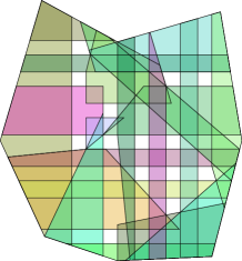
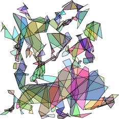
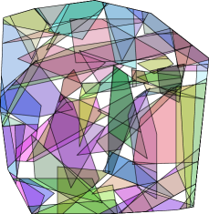
Figure 1: Solutions to maze_79_50_5_5, fpg-poly_400_h2, and cheese163 instances. The instances have $64$, $462$, and $163$ vertices and the solutions have $23$, $172$, and $68$ polygons, respectively.

Our general strategy consists of two distinct phases. First, we produce a large collection $\mathcal{C}$ of large convex polygons inside $P$. Second, we find a small subset $\SS\subseteq\mathcal{C}$ that covers $P$, which is returned as the solution. Figure 1 shows three small solutions and we can observe that most convex polygons are maximal and often much larger than necessary. Our approach is different from that of the winning team DIKU (AMW), that uses clique cover [1].

To construct the collection $\mathcal{C}$ in phase $1$, we used either a modified version of the Bron-Kerbosch algorithm or a randomized bloating procedure starting from a constrained Delaunay triangulation (Section 2). To solve the set cover problem in phase $2$, we used integer programming and simulated annealing. The key element for the efficiency of phase $2$ is to iteratively generate constraints as detailed in Section 3. Generally speaking, the initial constraints ensure that all input vertices are covered and supplementary constraints ensure that a point in each uncovered area is covered in the following iteration. In fact, to obtain our best solutions, we repeat phase $2$ using the union of the solutions from independent runs of the first two phases as the collection $\mathcal{C}$. Our results are discussed in Section 4.

2 Collections

We now describe phase $1$ of our strategy: building a collection. Throughout, the instance is a polygon with holes $P$ with vertex set $V$. Formally speaking, a collection $\mathcal{C}$ is defined exactly as a solution $\SS$: a finite set of convex polygons whose union is $P$. However, while we want a solution $\SS$ to have as few elements as possible, the most important aspect of a collection $\mathcal{C}$ is that it contains a solution $\SS\subseteq\mathcal{C}$ with few elements. Ideally, $|\mathcal{C}|$ is also not too big so the second phase solver is not overloaded, but the size of $\mathcal{C}$ is of secondary importance.

Given a set of points $S$, a convex polygon $C\subseteq P$ is $S$-maximal if the vertices of $C$ are in $S$ and there exists no point $s\in S$ with $\operatorname{conv}(C\cup\{s\})\subseteq P$. Next, we show how to build a collection with all $S$-maximal convex polygons.

Bron-Kerbosch

The Bron-Kerbosch algorithm [2] is a classic algorithm to enumerate all maximal cliques in a graph (in our case the visibility graph) with good practical performance [6]. The algorithm recursively keeps three sets:

• Vertices in the current maximal clique. Initially, $\mathtt{R}=\emptyset$.

• Vertices that may be added to the current maximal clique (these must be adjacent to all vertices in $\mathtt{R}$). Initially, $\mathtt{S}=S$.

• Vertices that may not be added to the current maximal clique because otherwise the same clique would be reported multiple times. Initially, $\mathtt{X}=\emptyset$.

If the polygon $P$ has no holes and $S$, then there is a bijection between the maximal cliques in the visibility graph of $S$ on $P$ and the $S$-maximal convex polygons. While this is no longer true in the version with holes, we can adapt the Bron-Kerbosch algorithm to enumerate all $S$-maximal convex polygons as shown in Listing LABEL:l:bk. Figure 3 shows how the number of $V$-maximal convex polygons grows for different instances and that we can compute all $V$-maximal convex polygons quickly for instances with around 10 thousand vertices.

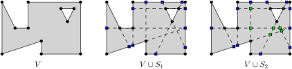
Figure 2: Definitions of $V$, $S_{1}$, and $S_{2}$.

Listing 1: Modified Bron-Kerbosch algorithm.

⬇

BronKerbosch(R, S, X):

if S and X are both empty: report conv(R) and return

if X $\cap$ conv(R) $\neq$ {}: return // Only for improved performance

for each vertex v in S:

S’ $\leftarrow$ X’ $\leftarrow$ {}

for each vertex u in S:

if v $\neq$ u and conv(R $\cup$ {u,v}) $\subseteq$ P: S’ $\leftarrow$ S’ $\cup$ {u}

for each vertex u in X:

if v $\neq$ u and conv(R $\cup$ {u,v}) $\subseteq$ P: X’ $\leftarrow$ X’ $\cup$ {u}

BronKerbosch(R $\cup$ {v}, S’, X’)

S $\leftarrow$ S \ {v}, X $\leftarrow$ X $\cup$ {v}

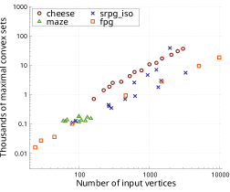
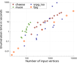
Figure 3: Number of $V$-maximal convex polygons and the time to enumerate them.

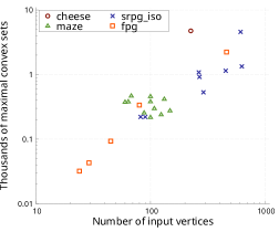
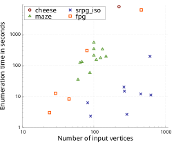
Figure 4: Number of $(V\cup S_{1})$-maximal convex polygons and the time to enumerate them.

Let $S_{1}$ be the set of the endpoints of the largest segments inside $P$ that contain each edge of $P$ (Figure 2). It is easy to see that $|S_{1}|\leq 2|V|$. However, as shown in Figure 4, we are only able to compute all $(V\cup S_{1})$-maximal convex polygons for instances with less than one thousand vertices. It is possible that a modified version of the Bron-Kerbosch algorithm gives better results, either by using a pivot or choosing a particular order for the points, but we have not succeeded in obtaining significant improvements. Another natural set of points is the set $S_{2}\supseteq S_{1}$ defined as the intersection points (inside $P$) of the lines containing the edges of $P$ (Figure 2). The set $S_{2}$ may however have size roughly $|V|^{2}$. Hence, computing all $(V\cup S_{2})$-maximal convex polygons is only feasible for very small instances.

Random Bloating

As a $V$-maximal convex polygon $C$ is generally not $P$-maximal, we also grow $C$ with an operation we call bloating. Given a convex polygon $C$ and a set of points $S$, we construct an $S$-bloated convex polygon $C^{\prime}$ by iteratively trying to add a random point from $S$ to $C$ and taking the convex hull, verifying at each step that $C^{\prime}$ lies inside the instance polygon $P$. There are two sets of points that may compose $S$. First, $S_{1}(C)$ is the set of endpoints of the largest segment in $P$ that contains each edge of $C$. Second, $S_{2}(C)$ is the union of $S_{1}(C)$ and the intersection points of the lines containing the edges of $C$, if the points are inside $P$. Notice that $|S_{1}(C)|=O(|C|)$, but $|S_{2}(C)|=O(|C|^{2})$.

To start the bloating operation, we need a convex polygon $C$. One approach is to use the $V$-maximal convex polygons produced by Bron-Kerbosch. A much faster approach for large instances is to use a constrained Delaunay triangulation of the instance polygon. In this case, we start by $V$-bloating the triangles into a convex polygon $C$, and then possibly $S_{1}(C)$-bloating or $S_{2}(C)$-bloating the polygon $C$. Since the procedure is randomized, we can replicate the triangles multiple times to obtain larger collections of large convex polygons.

3 Set Cover

Given a collection $\mathcal{C}$ of convex polygons that covers $P$, our covering problem consists of finding a small subset of $\mathcal{C}$ that still covers $P$. In contrast to the classic set cover problem, in our case $P$ is an infinite set of points. Nevertheless, it is easy to create a finite set of witnesses $W$, that satisfy that $W$ is covered by a subset $\SS$ of $\mathcal{C}$ if and only if $P$ is. To do that, we place a point inside each region (excluding holes) of the arrangement of line segments defining the boundaries of the polygons in $\mathcal{C}$ and $P$ (Figure 5(a)). The size of such set $W$ is however very large in practice and potentially quadratic in the number of segments of $\mathcal{C}$.

Producing small sets of witnesses has been studied in the context of art gallery problems [3]. However, we do not know if small sets of witnesses exist for our problem. Hence, we use a loose definition of witness as any finite set of points $W\subset P$. In practice, we want $W$ to be such that if $W$ is covered, then most of $P$ is covered. Next, we show how to build such set of witnesses and afterwards we describe how we solved the finite set cover problem.

Witnesses

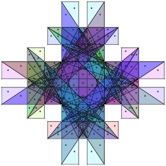
(a)                                                          (b)

Figure 5: All the 82 $V$-maximal convex polygons for the socg_fixed60 instance with (a) the 1009 arrangement witnesses and (b) the 200 vertex witnesses.

A set of witnesses $W$ that gave very good results, which we call vertex witnesses, consists of one witness inside each cell of the arrangement that contains a vertex of the instance polygon $P$, as shown in Figure 5(b). This set guarantees that if $W$ is covered, then all points that are arbitrarily close to the vertices of $P$ are covered. However, trivially computing $W$ requires building the arrangement of the collection $\mathcal{C}$, which is too slow and memory consuming for large $\mathcal{C}$.

A set of witnesses $W$ that also gives excellent results and is much faster to compute is called quick vertex witnesses. For each vertex $v$ of $P$, we consider all edges in $\mathcal{C}$ and also $P$ that are adjacent to $v$. We order these edges around $v$ starting and ending with the edges of $P$. For each pair of consecutive edges, we add a point $w$ to $W$ that is between the two consecutive edges and infinitely close to $v$. Notice that the number of vertex witnesses is linear in the number of edges of $\mathcal{C}$ and it can also be built in near linear time, avoiding the construction of the whole arrangement of $\mathcal{C}$. If $P$ has not colinear points, then the quick vertex witnesses give the same vertex coverage guarantee as the vertex witnesses. We represent points that are arbitrarily close to $v$ implicitly as a point and a direction.

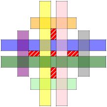
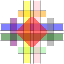
(a)                                         (b)

Figure 6: (a) A solution that covers all vertex witnesses of the socg_fixed60 instance but not the whole polygon. Uncovered regions are marked in striped red. (b) The optimal solution obtained from the previous one by merging the uncovered regions.

Given a set $\SS^{\prime}$ of convex polygons that cover $W$, there are two natural options to produce a valid solution $\SS$. The first option is to make $\SS=\SS^{\prime}\cup\mathcal{R}$ for a set $\mathcal{R}$ built as follows. The uncovered region $P\setminus\cup_{C\in\SS^{\prime}}C$ consists of a set $\mathcal{U}$ of disjoint polygons, possibly with holes (Figure 6(a)). However, most of the time the polygons in $\mathcal{U}$ are in fact convex. For each polygon $U\in\mathcal{U}$, if $U$ is convex, then we add $U$ to $\mathcal{R}$. Otherwise, we triangulate $U$ and add the triangles to $\mathcal{R}$. Furthermore, we can greedily merge convex polygons in $\mathcal{R}$ to reduce their number, as long as the convex hull of the union remains inside $P$, which works very well for the SoCG logo solution shown in Figure 6(b).

A second option is normally preferable and is based on the constraint generation technique, widely used in integer programming. We build the set $\mathcal{R}$ as before, but for each convex polygon $R\in\mathcal{R}$ we add to $W$ a point inside $R$. Then, we run the solver again and repeat until a valid solution is found (or one with a very few uncovered regions). It is perhaps surprising how few iterations are normally needed, as shown in Figure 7.

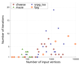
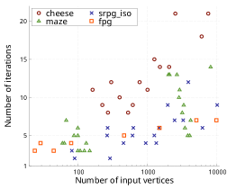
(a)                                                      (b)

Figure 7: Number of iterations to find a valid solution starting from quick vertex witnesses using IP as the solver, setting $\mathcal{C}$ as (a) all $V$-maximal convex polygons and (b) $2$ times triangulation $(V\cup S_{2}(C))$-bloated convex polygons.

Set Cover Solver

A simple and often efficient way to solve a set cover problem $(W,\mathcal{C})$ is to model the problem as integer programming (IP) and then use the CPLEX solver [4]. Each set in $\mathcal{C}$ becomes a binary variable and each witness point $w\in W$ becomes a constraint forcing the sum of the sets that contain $w$ to be at least $1$. As discussed in the next section, this approach can optimally solve fairly large problems in seconds and give good approximation guarantees to some extremely large problems. However, for some large problems the solution found is extremely bad (sometimes worse than a greedy algorithm).

Another solver we used is based on simulated annealing. We start from a greedy solution, obtained by adding to $\SS$ the convex polygon that covers the most uncovered witnesses at each step, breaking ties randomly. If a previously added convex polygon in $\SS$ becomes unnecessary, we remove it from $\SS$. At each step, we remove $3$ random convex polygons from $\SS$ and use the same greedy approach to make the solution cover all $W$. A larger solution is accepted with a certain probability that depends on the size difference and decreases as we advance in the annealing procedure. This simple procedure normally produces solutions that are close to the IP solutions, and sometimes produce much better solutions.

4 Results

We now discuss the quality of the solutions obtained for each technique. Our C++ code uses CGAL [8] and CPLEX [4] and is run on Fedora Linux on a Dell Precision 7560 laptop with an Intel Core i7-11850H and 128GB of RAM. All times refer to a single core execution with scheduling coordinated by GNU Parallel [7]. Our plots for a solution $\SS$ use the relative solution size, defined as $|\SS^{*}|/|\SS|$, where $\SS^{*}$ is the best solution submitted among all teams. This corresponds to the square root of the Challenge score of $\SS$.

Figure 8 compares the different techniques to obtain $V$-maximal convex polygons before bloating them. As the figure shows, using $4$ replications of each constrained Delaunay triangle gives solutions that are almost as good as Bron-Kerbosch, but works on all instance sizes. Hence, we use this setting for Figures 9 and 10.

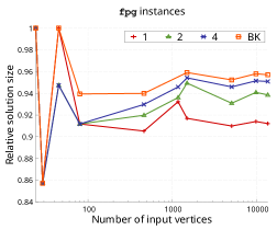
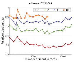
Figure 8: Solution sizes relative to the best Challenge solution. Data is based on a triangulation replicated $1$, $2$, or $4$ times and randomly bloated using $V$. Alternatively, we use Bron-Kerbosch (BK) to obtain all $V$-maximal polygons, when the running time is not too long. Afterwards, all collections have bloated again using $V\cup S_{2}(C)$ and solved using IP.

Figure 9 shows the relative solution sizes using different bloating approaches and comparing the simulated annealing and the IP solvers. You can see that the simulated annealing solver is only slightly worse than IP for small instances, but better for large cheese instances. We limited the running time of IP to 10 minutes per iteration. The total running times of the solvers are compared in Figure 10.

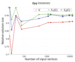
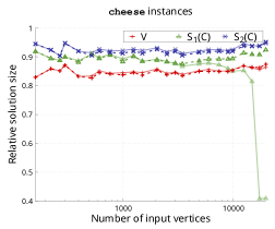
Figure 9: Solution sizes relative to the best Challenge solution. A solid line is used for the IP solver and a dashed line for simulated annealing. Data is based on a triangulation randomly bloated using $V$ (red) and then bloated again using $V\cup S_{1}(C)$ (green), or $V\cup S_{2}(C)$ (blue).

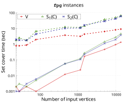
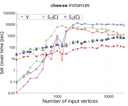
Figure 10: Running times in seconds of the set cover solvers used to find the solutions of Figure 9.

A much better collection is obtained by using the union of several high quality solutions as a collection. To produce the previous plots, we performed $3$ independent runs for each settings (showing the best result found). Figure 11 shows the solution sizes obtained by using the best $k$ solutions from these runs as the collection.

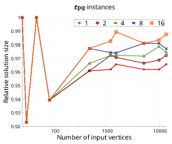
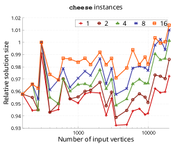
Figure 11: Relative solution sizes merging the $k$ best solutions for different values of $k$.

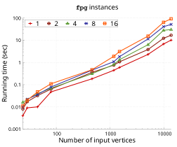
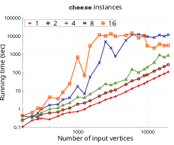
Figure 12: Running times in seconds to find the solutions of Figure 11.

References

- [1] Mikkel Abrahamsen, William B. Meyling, and André Nusser. Constructing concise convex covers via clique covers. In 39th International Symposium on Computational Geometry (SoCG 2023), volume 258, pages 62:1–62–9, 2023.
- [2] Coen Bron and Joep Kerbosch. Algorithm 457: finding all cliques of an undirected graph. Communications of the ACM, 16(9):575–577, 1973.
- [3] Kyung-Yong Chwa, Byung-Cheol Jo, Christian Knauer, Esther Moet, René Van Oostrum, and Chan-Su Shin. Guarding art galleries by guarding witnesses. International Journal of Computational Geometry & Applications, 16(02n03):205–226, 2006.
- [4] IBM ILOG CPLEX. V22.1: User’s manual for CPLEX. International Business Machines Corporation, 2023.
- [5] Sándor P. Fekete, Phillip Keldenich, Dominik Krupke, and Stefan Schirra. Minimum coverage by convex polygons: The CG:SHOP challenge 2023, 2023. URL: https://arxiv.org/abs/2303.07007, arXiv:2303.07007.
- [6] Ina Koch. Enumerating all connected maximal common subgraphs in two graphs. Theoretical Computer Science, 250(1-2):1–30, 2001.
- [7] O. Tange. Gnu parallel - the command-line power tool. ;login: The USENIX Magazine, 36(1):42–47, Feb 2011. URL: http://www.gnu.org/s/parallel.
- [8] The CGAL Project. CGAL User and Reference Manual. CGAL Editorial Board, 5.5.1 edition, 2022. URL: https://doc.cgal.org/5.5.1/Manual/packages.html.