Optimal Power System Topology Control
Under Uncertain Wildfire Risk

Abstract

Wildfires pose a significant threat to the safe and reliable operation of electric power systems. They can quickly spread and cause severe damage to power infrastructure. To reduce the risk, public safety power shutoffs are often used to restore power balance and prevent widespread blackouts. However, the unpredictability of wildfires makes it challenging to implement effective counter-measures in a timely manner. This paper proposes an optimization-based topology control problem as a solution to mitigate the impact of wildfires. The goal is to find the optimal network topology that minimizes total operating costs and prevents load shedding during power shutoffs under uncertain line shutoff scenarios caused by uncertain spreading wildfires. The solution involves solving two-stage stochastic mixed-integer linear programs, with preventive and corrective control actions taken when the risk of a wildfire and corresponding outage line scenarios are known with low and high confidence, respectively. The Progressive Hedging algorithm is used to solve both problems. The effectiveness of the proposed approach is demonstrated using data from the RTS-GMLC system that is artificially geo-located in Southern California, including actual wildfire incidents and risk maps. Our work provides a crucial study of the comparative benefits due to accurate risk forecast and corresponding preventive control over real-time corrective control that may not be realistic.

I Introduction

Effective wildfire mitigation has become a pressing challenge for reliable power system operations in recent years. Due to climate change, the number and severity of wildfires have increased significantly. In the United States in 2021, there were over 58,000 wildfires that burned more than 7.13 million acres [1]. From 2019 to 2021, the number of wildfire cases increased by 16.9% and the number of acres burned increased by 51.1%. Wildfires can be caused by various factors such as lightning, arson, power line faults, and campfires [2]. Once ignited, they can spread quickly, up to 10-15 mph, causing destruction to infrastructure along their path. Power transmission lines located in high-risk areas are especially vulnerable to wildfire damage, including the burning of wood poles and damage to steel towers and transmission lines. Additionally, dense smoke from nearby wildfires can contaminate the insulating medium of transmission lines, leading to line outages [3] and power shutoffs in affected communities. To prevent and minimize the disruption of electricity delivery caused by wildfires, effective control approaches in the power grid are crucial.

In an effort to mitigate ongoing wildfires and prevent future consequences, de-energization of system components, such as transmission lines and loads, has been recognized as a well-established solution known as the Public Safety Power Shutoff (PSPS). As power shutoff can have an economic impact and raise concerns over system reliability, the focus of many research works has been on designing an optimal shutoff plan in recent years. Depending on the optimization framework design, these problems generally include maximizing load delivery [4, 5], minimizing system risks [6, 7, 8, 9, 10], and enhancing grid resilience [11, 12, 13]. Although these approaches are well-suited for optimally switching lines under a given wildfire or designing a network topology to minimize potential wildfires, the majority of existing optimization models are deterministic and do not consider the uncertainty associated with wildfire risk models. One critical issue is that the forecast for wildfire risk can evolve over a time-period of several days to a week [14], and may change the set of transmission lines included in the preventive shut-off (PSPS). This uncertainty can render control strategies planned for deterministic shut-offs fail to securely and reliably reduce load outages. Recently, a robust decision-making framework was proposed [15] for highly renewable power systems to deal with the wildfire threat. However, a stochastic fire spread simulation needs to be conducted before the model can be applied. The problem of optimal control design, in both planning and operations, for developing wildfires with changing risks remains open. Addressing this problem will help quantify the effect that the accuracy of wildfire risk forecast has on control algorithms and the size of resulting load-shutoffs. Although our framework is generalizable to other control efforts, this paper focuses specifically on the design of optimal topology control.

The goal of this paper is to present an optimal topology control strategy under uncertain line outages caused by wildfires. To incorporate the line outage uncertainty, we propose a two-stage stochastic mixed-integer programming formulation where multiple wildfire (and line outage) scenarios are considered based on the current wildfire risk map. The problem utilizes existing resources like generation ramping, load shedding, line switching, etc. to mitigate the evolving wildfire risk, and further to minimize the total operating cost, and reduce load shedding. We present both preventive and corrective control schemes for wildfire mitigation with the two strategies differing in when the mitigation strategies are implemented. Specifically, the preventive control seeks to find an optimal network topology in advance (i.e., at the first stage of the two-stage stochastic program) to mitigate the different wildfire scenarios that may arise under the risk map. In contrast, the corrective control allows for different network configurations in the second stage of the two-stage stochastic program for each imminent wildfire scenario. We compare the load shedding and the generation cost due to the preventive and corrective control strategies using two sets of wildfire risk: one where the outage scenarios generated by the wildfire risk are more disperse, i.e., the confidence on these scenarios are low, and the other where the scenarios are concentrated in a smaller geographical region, arising from a more accurate wildfire risk prediction. Our results show that preventive policies that can be implemented ahead of time have similar performance as optimal corrective actions (that may not be realistic) in settings where the risk is more concentrated. We solve both versions of the stochastic optimization problem using the Progressive Hedging (PH) algorithm [16] and show that the sub-problems in either setting are parallelizable and hence solvable even when the number of scenarios may be greater than hundred.

The rest of the paper is organized as follows. Section sec:nomenclature presents the notations while Section III introduces the deterministic topology control problem using a DC power flow model. Section IV presents the preventive control formulation. The corrective control problem is formulated is Section V. Section VI presents an overview of the PH algorithm that is applied to both the preventive and the corrective control formulations. Numerical experiments using the RTS-GMLC systems are presented in Section VII to corroborate the effectiveness and efficiency of the proposed algorithms. Conclusions and possible avenues for future work of our work are presented in Section VIII.

II Nomenclature

This section presents nomenclature and terminology, including those that are well understood and used routinely in the power systems literature. Unless otherwise stated, all the physical values are in per-unit (p.u.).

Sets:
$\mathcal{N}$ - set of buses in the network
$\mathcal{N}(i)$ - set of buses connected to bus $i$ by an line
$\mathcal{E}$ - set of lines in the network
$\mathcal{S}$ - set of line outage scenarios
$\mathcal{\tilde{E}}_{s}$ - set of damaged lines in scenario $s$
$\mathcal{E}_{s}$ - set of operational edges for scenario $s$
Parameters:
$\bm{p}^{d}_{i}$ - real power demand at bus $i$
$\bm{c}_{i}$ - cost of generating 1 MW in bus $i$
$\bm{c}^{r}_{i}$ - cost of ramping 1 MW in bus $i$
$\bm{c}^{\text{voll}}_{i}$ - value of lost load (VoLL) at bus $i$
$\bm{Y}_{ij}=\bm{g}_{ij}+\bm{j}\bm{b}_{ij}$ - admittance of line $(i,j)$
$(\bm{p}^{gl}_{i},\bm{p}^{gu}_{i})$ - bounds for active power generated at bus $i$
$\bm{\theta}_{ij}^{\Delta}$ - maximum phase angle difference across line$(i,j)$
$\bm{t}_{ij}$ - thermal limit of line $(i,j)$
$\bm{r}$ - reference bus
$\bm{\theta}\triangleq\bm{\theta}_{ij}^{\Delta}\cdot|\mathcal{E}|$ - big $\bm{M}$ value for phase angle difference
$\bm{\beta}$ - budget on the number of lines that can be controlled
$\bm{m}$ - maximum number of line outages for each scenario

III System Modeling

We first present the optimal topology control problem on a transmission system using the DC power flow model [17].

III-A Deterministic Topology Control

To that end, let the variables $\theta_{i}$ and $p_{i}^{g}$ denote the voltage phase angle and the real power generated at bus $i\in\mathcal{N}$, respectively. Per line $(i,j)\in\mathcal{E}$,let $p_{ij}$ and $\theta_{ij}\triangleq\theta_{i}-\theta_{j}$ denote the active power flow and the phase angle difference, respectively. We also let $\bm{p}^{d}$, $\bm{p}^{g}$ denote the vector of demands and generations over all the buses in the system. The optimal topology control problem[18] seeks to determine the optimal network topology so that the total generation cost to meet all the demands in $\bm{p}^{d}$ is minimized. For ease of exposition, we assume that the generation costs are linear. Furthermore, to model the topology switching action, we introduce additional binary decision variables $z_{ij}$ for every $(i,j)\in\mathcal{E}$ that takes a value $1$ (or $0$) when the line $(i,j)$ is closed (or open). This way, a Mixed-Integer Linear Program (MILP) can be formulated as follows:

$$\min\quad\sum_{i\in\mathcal{N}}\bm{c}_{i}\cdot p_{i}^{g}\quad\text{ subject to:}$$ (1a)

$$\theta_{\bm{r}}=0$$ (1b)

$$p_{i}^{g}\in[p_{i}^{gl},p_{i}^{gu}]\quad\forall i\in\mathcal{N}$$ (1c)

$$p_{i}^{g}-\bm{p}_{i}^{d}=\sum_{(i,j)\in{\mathcal{E}}}p_{ij}-\sum_{(j,i)\in{\mathcal{E}}}p_{ji}\quad\forall i\in\mathcal{N}$$ (1d)

$$p_{ij}\in[-\bm{t}_{ij}z_{ij},\bm{t}_{ij}z_{ij}]\quad\forall(i,j)\in\mathcal{E}$$ (1e)

$$p_{ij}\geqslant-\bm{b}_{ij}\left(\theta_{ij}+\bm{\theta}(1-z_{ij})\right)\quad\forall(i,j)\in\mathcal{E}$$ (1f)

$$p_{ij}\leqslant-\bm{b}_{ij}\left(\theta_{ij}-\bm{\theta}(1-z_{ij})\right)\quad\forall(i,j)\in\mathcal{E}$$ (1g)

$$\sum_{(i,j)\in\mathcal{E}}(1-z_{ij})\leqslant\bm{\beta}$$ (1h)

$$z_{ij}\in\{0,1\}\quad\forall(i,j)\in\mathcal{E}$$ (1i)

where (1b) sets the voltage phase angle at the reference bus to zero and (1c) limits the active power generation at each bus. The constraint (1d) enforces the power balance at each bus in the network. The constraint (1e) enforces the active power flowing on a line to be zero (bounded by its thermal limits) when the line is open (closed) i.e., $z_{ij}=0$ ($z_{ij}=1$).The constraints (1f) and (1g) together enforce the DC power flow constraint for each line $(i,j)$ if it is closed. Finally, (1h) limits the number of lines that can be switched open using a budget of $\bm{\beta}$. In this context, we remark that though the DC power flow model is adopted in this paper for formulating the topology control problem, extension of the problem to include the full AC power flow equations can be done by leveraging existing relaxation-based techniques [19], or a post-selection AC power flow analysis [20] for feasibility. We delegate these generalizations for future work.

III-B Modeling line outage uncertainty

An accurate model to forecast the line outage scenarios under a given wildfire risk map is extremely important for the problem of determining an optimal mitigation strategy. Though our model can incorporate outages on all possible types of components in a transmission system, we restrict our attention to line outages for ease of presentation and exposition. Here, we resort to a scenario-based line outage uncertainty model for the set $\mathcal{S}$ that contains line outage scenarios that are likely due to a given wildfire risk map. For outage scenario $s\in\mathcal{S}$, $\xi_{ij}^{s}$ takes a value $0$ or $1$ if the line $(i,j)\in\mathcal{E}$ is not outaged or outaged, respectively. These outages are generated using a probability that is obtained from fragility models that map factors like temperature, wind, fuels, land topography, starting location for the fire, as well as the operator’s shut-off policy for the risk of impending fires [6]. The development and validation of fragility models to obtain these risks are beyond our scope. In this work, we use existing wildfire risk values to generate possible scenarios directly, with a maximum number $\bm{m}$ of line outages per scenario. To model differing confidence in the wildfire risk, we consider a risk-threshold $\bm{R}$ (detailed in Section VII-A) that selects outages only amongst lines with risk value greater than $\bm{R}$. The setting where the wildfire risk map is known with high (low) confidence or when the mitigation problem is solved close (much farther away) in time from the wildfire ignition, can be modeled by setting $\bm{R}$ to high (low) values, respectively. Alternatively, for constant $\bm{R}$, increasing $|\mathcal{S}|$ (number of scenarios) improves the robustness of the solution to out-of-sample data.

We will next present two topology control schemes, namely preventive control and corrective control, as effective two-stage wildfire mitigation solutions. The preventive control scheme seeks an optimal topology ahead of the wildfire uncertainty realization, while the corrective control scheme allows for reconfiguring flexible network topology control for each individual uncertainty realization. Notably, both of these methods are amenable to efficiently applying decomposition/relaxation techniques. Both methods and highlights of our approach are depicted in Fig. 1.

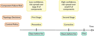
Figure 1: Primary differences in variables, time-frame and risks for preventive and corrective control policies.

IV Preventive Control Formulation

In this section, we formulate the preventive control mitigation strategy as a two-stage stochastic program [21], by performing the decision-making in two stages. The first stage decisions are referred to as the here-and-now decisions which are usually taken before the uncertainty, i.e., the outage scenario, is realized. The second stage decisions are referred to as the wait-and-see or recourse decisions; that is, these decisions are made upon realization of the actual outage scenario. For the preventive control problem, the first stage decisions include the generation levels for each generator in the system and the topology decisions on the transmission lines. The second stage decisions are post-outage variables including the phase angle at the buses, the active power flow on the lines, the ramping provided by each generator and the amount of load shed at each load bus. Hence, the second stage decision is a function of the specific outage scenario $s\in\mathcal{S}$.

Before we present the formulation, we first introduce notations for each decision variable in the problem. To that end, we let $p_{i}^{g}$ denote the active power generation at the bus $i\in\mathcal{N}$. To capture the initial on-off status of each line, we partition the set $\mathcal{E}$ into $\mathcal{E}^{\text{on}}$ and $\mathcal{E}^{\text{off}}$, which respectively contain the set of lines that are initially closed and open. Associated with each line in $\mathcal{E}^{\text{on}}$ and $\mathcal{E}^{\text{off}}$, we introduce binary variables, $z_{ij}^{\text{on}}$ and $z_{ij}^{\text{off}}$, respectively, to model topology switching status. For every $(i,j)\in\mathcal{E}^{\text{on}}$, $z_{ij}^{\text{on}}=1$ (or alternatively, $z_{ij}^{\text{on}}=0$) when $(i,j)$’s status is changed to open (or alternatively, is left closed). Similarly, For every $(i,j)\in\mathcal{E}^{\text{off}}$, $z_{ij}^{\text{off}}=1$ (or alternatively, $z_{ij}^{\text{off}}=0$) when $(i,j)$’s status is changed to closed (or alternatively, is left open). The distinction between $z_{ij}^{\text{on}}$ and $z_{ij}^{\text{off}}$ is explicitly made to model different initial grid topology states. In summary, the first stage decision variables are given by the set $\{(p_{i}^{g}),(z_{ij}^{\text{on}}),(z_{ij}^{\text{off}})\}$. Corresponding to each outage scenario $s\in\mathcal{S}$, we let $\theta_{i}^{s}$, $r_{i}^{s}$, and $\ell_{i}^{s}$ denote the voltage phase angle, the ramping, and the load shed at the bus $i\in\mathcal{N}$. With regards to ramping, without loss of generality, we assume all generators can provide either up or down ramping. Additionally, for each outage scenario $s\in\mathcal{S}$, we let $p_{ij}^{s}$ and $\theta_{ij}^{s}\triangleq\theta_{i}^{s}-\theta_{j}^{s}$ denote the active power flow and the phase angle difference for each line $(i,j)\in\mathcal{E}$. The second stage decision variables are summarized by the set $\{(\theta_{i}^{s}),(r_{i}^{s}),(\ell_{i}^{s}),(p_{ij}^{s}),(\theta_{ij}^{s})\}$. Finally, we also let $\mathbb{E}[\cdot]$ denote the expectation operator taken over the discrete set of outage scenarios. For simplicity, we will assume that all the scenarios in the set $\mathcal{S}$ are equally likely i.e., $\operatorname{Pr}(s)=\pi_{s}=|\mathcal{S}|^{-1}$. With these notations, we now present the optimization problem formulation for the preventive control strategy as follows:

$$\min\quad\sum_{i\in\mathcal{N}}\bm{c}_{i}\cdot p_{i}^{g}+\mathbb{E}\left[\sum_{i\in\mathcal{N}}\left(\bm{c}^{r}_{i}\cdot r_{i}^{s}+\bm{c}^{\text{voll}}_{i}\cdot\ell_{i}^{s}\right)\right]$$ (2a)

first stage variables & constraints:

$$p_{i}^{g}\in[p_{i}^{gl},p_{i}^{gu}]\quad\forall i\in\mathcal{N}$$ (2b)

$$z_{ij}^{\text{on}}\in\{0,1\}\quad\forall(i,j)\in\mathcal{E}^{\text{on}}$$ (2c)

$$z_{ij}^{\text{off}}\in\{0,1\}\quad\forall(i,j)\in\mathcal{E}^{\text{off}}$$ (2d)

$$\sum_{(i,j)\in\mathcal{E}^{\text{on}}}z_{ij}^{\text{on}}+\sum_{(i,j)\in\mathcal{E}^{\text{off}}}z_{ij}^{\text{off}}\leqslant\bm{\beta}$$ (2e)

second stage variables & constraints $$\forall s\in\mathcal{S}$$:

$$\theta^{s}_{\bm{r}}=0\quad$$ (2f)

$$p_{i}^{g}+r_{i}^{s}\in[p_{i}^{gl},p_{i}^{gu}]\quad\forall i\in\mathcal{N}$$ (2g)

$$\ell_{i}^{s}\in[0,\bm{p}_{i}^{d}]\quad\forall i\in\mathcal{N}$$ (2h)

$$p_{i}^{g}+r_{i}^{s}-(\bm{p}_{i}^{d}-\ell_{i}^{s})=\sum_{(i,j)\in\mathcal{E}_{s}}p_{ij}^{s}-\sum_{(j,i)\in\mathcal{E}_{s}}p_{ji}^{s}\quad\forall i\in\mathcal{N}$$ (2i)

$$p_{ij}^{s}\in[-\bm{t}_{ij}\xi_{ij}^{s}(1-z_{ij}^{\text{on}}),\bm{t}_{ij}\xi_{ij}^{s}(1-z_{ij}^{\text{on}})]\leavevmode\nobreak\ \forall(i,j)\in\mathcal{E}^{\text{on}}$$ (2j)

$$p_{ij}^{s}\in[-\bm{t}_{ij}\xi_{ij}^{s}z_{ij}^{\text{off}},\bm{t}_{ij}\xi_{ij}^{s}z_{ij}^{\text{off}}]\leavevmode\nobreak\ \forall(i,j)\in\mathcal{E}^{\text{off}}$$ (2k)

$$p_{ij}^{s}+\bm{b}_{ij}\left\{\theta_{ij}^{s}+\bm{\theta}\left(1-\xi_{ij}^{s}(1-z_{ij}^{\text{on}})\right)\right\}\geqslant 0\quad\forall(i,j)\in\mathcal{E}^{\text{on}}$$ (2l)

$$p_{ij}^{s}+\bm{b}_{ij}\left\{\theta_{ij}^{s}-\bm{\theta}\left(1-\xi_{ij}^{s}(1-z_{ij}^{\text{on}})\right)\right\}\leqslant 0\quad\forall(i,j)\in\mathcal{E}^{\text{on}}$$ (2m)

$$p_{ij}^{s}+\bm{b}_{ij}\left\{\theta_{ij}^{s}+\bm{\theta}\left(1-\xi_{ij}^{s}z_{ij}^{\text{off}}\right)\right\}\geqslant 0\quad\forall(i,j)\in\mathcal{E}^{\text{off}}$$ (2n)

$$p_{ij}^{s}+\bm{b}_{ij}\left\{\theta_{ij}^{s}-\bm{\theta}\left(1-\xi_{ij}^{s}z_{ij}^{\text{off}}\right)\right\}\leqslant 0\quad\forall(i,j)\in\mathcal{E}^{\text{off}}$$ (2o)

The optimization problem in (2) aims to minimize the sum of the nominal generation costs, the expected ramping costs, and the expected value of lost load over all the outage scenarios. The cost coefficients can be set up to accommodate different system design needs, such as prioritization of nominal generation over ramping and load shed, or the other way around; the actual cost coefficients that are used for the formulation are discussed in Section VII. Under a budget of switching at most $\bm{\beta}$ lines, constraints in (2b) – (2e) represent the limits on the first stage decision variables. The second stage constraints in (2f) – (2o) enforce the operating limits for the second stage variables and the post-outage DC power flow physics depending on the active status of the lines. The line switching operations $z_{ij}^{\text{on}}$ and $z_{ij}^{\text{off}}$ are coupled with the line outage scenarios $\xi_{ij}^{s}$ to compute the active status of line $(i,j)$ for scenario $s\in\mathcal{S}$. Specifically, the thermal limits in (2j) – (2k) and the DC power flow constraints in (2l) – (2o) for a line $(i,j)\in\mathcal{E}$ are enforced only under the following two conditions: (1) $\xi_{ij}^{s}=1$, $(1-z_{ij}^{\text{on}})=1$ with $(i,j)\in\mathcal{E}^{\text{on}}$ or (2) $\xi_{ij}^{s}=1$, $z_{ij}^{\text{off}}=1$ with $(i,j)\in\mathcal{E}^{\text{off}}$. In all other cases, trivial bounds using big $\bm{M}$ constraints are enforced.

V Corrective Control Formulation

In contrast to the preventive control formulation where the budget-constrained topology control are first-stage decisions, the corrective control focuses on deciding on the topology control actions in the recourse (or second-stage) problem. The rationale behind this choice is that performing topology control once the wildfire-related outage scenario is realized or known with certainty, provides more flexibility and can aid in achieving better cost reduction in terms of ramping and load shed. Note that such near real-time control may not be possible and requires excellent wildfire forecast and fast communications. Nonetheless, we present the formulation for the two-stage corrective control problem below and compare its performance with preventive control later:

$$\min\quad\sum_{i\in\mathcal{N}}\bm{c}_{i}\cdot p_{i}^{g}+\mathbb{E}\left[\sum_{i\in\mathcal{N}}\left(\bm{c}^{r}_{i}\cdot r_{i}^{s}+\bm{c}^{\text{voll}}_{i}\cdot\ell_{i}^{s}\right)\right]$$ (3a)

first stage variables & constraints: Eq. (2b)

second stage variables & constraints $$\forall s\in\mathcal{S}$$:

Eqs. (2f), (2g), (2h), (2i), and

$$z_{ij}^{\text{on},s}\in\{0,1\}\quad\forall(i,j)\in\mathcal{E}^{\text{on}}$$ (3b)

$$z_{ij}^{\text{off},s}\in\{0,1\}\quad\forall(i,j)\in\mathcal{E}^{\text{off}}$$ (3c)

$$\sum_{(i,j)\in\mathcal{E}^{\text{on}}}z_{ij}^{\text{on},s}+\sum_{(i,j)\in\mathcal{E}^{\text{off}}}z_{ij}^{\text{off},s}\leqslant\bm{\beta}$$ (3d)

$$p_{ij}^{s}\in[-\bm{t}_{ij}\xi_{ij}^{s}(1-z_{ij}^{\text{on},s}),\bm{t}_{ij}\xi_{ij}^{s}(1-z_{ij}^{\text{on},s})]\leavevmode\nobreak\ \forall(i,j)\in\mathcal{E}^{\text{on}}$$ (3e)

$$p_{ij}^{s}\in[-\bm{t}_{ij}\xi_{ij}^{s}z_{ij}^{\text{off},s},\bm{t}_{ij}\xi_{ij}^{s}z_{ij}^{\text{off},s}]\leavevmode\nobreak\ \forall(i,j)\in\mathcal{E}^{\text{off}}$$ (3f)

$$p_{ij}^{s}+\bm{b}_{ij}\left\{\theta_{ij}^{s}+\bm{\theta}\left(1-\xi_{ij}^{s}(1-z_{ij}^{\text{on},s})\right)\right\}\geqslant 0\leavevmode\nobreak\ \forall(i,j)\in\mathcal{E}^{\text{on}}$$ (3g)

$$p_{ij}^{s}+\bm{b}_{ij}\left\{\theta_{ij}^{s}-\bm{\theta}\left(1-\xi_{ij}^{s}(1-z_{ij}^{\text{on},s})\right)\right\}\leqslant 0\leavevmode\nobreak\ \forall(i,j)\in\mathcal{E}^{\text{on}}$$ (3h)

$$p_{ij}^{s}+\bm{b}_{ij}\left\{\theta_{ij}^{s}+\bm{\theta}\left(1-\xi_{ij}^{s}z_{ij}^{\text{off},s}\right)\right\}\geqslant 0\leavevmode\nobreak\ \forall(i,j)\in\mathcal{E}^{\text{off}}$$ (3i)

$$p_{ij}^{s}+\bm{b}_{ij}\left\{\theta_{ij}^{s}-\bm{\theta}\left(1-\xi_{ij}^{s}z_{ij}^{\text{off},s}\right)\right\}\leqslant 0\leavevmode\nobreak\ \forall(i,j)\in\mathcal{E}^{\text{off}}$$ (3j)

The first-stage and second-stage decision variables for the above formulation are given by the sets $\{(p_{i}^{g})\}$ and $\{(z_{ij}^{\text{on},s}),(z_{ij}^{\text{off},s}),(\theta_{i}^{s}),(r_{i}^{s}),(\ell_{i}^{s}),(p_{ij}^{s}),(\theta_{ij}^{s})\}$, respectively. For each outage scenario $s\in\mathcal{S}$, the definitions of $z_{ij}^{\text{on},s}$ for $(i,j)\in\mathcal{E}^{\text{on}}$ and $z_{ij}^{\text{off},s}$ for $(i,j)\in\mathcal{E}^{\text{off}}$ are similar to the corresponding ones in Section IV. The only difference between the preventive and the corrective control formulations is that the corrective control problem has binary decision variables (topology control) only in the second stage while the preventive has them only the first stage. Mathematically, this makes the corrective control a more challenging problem to solve to global optimality with a strong need for heuristics. This is unlike the preventive control problem that can be solved to global optimality using standard techniques like Bender’s decomposition [22] or the Progressive Hedging (PH) algorithm [16]. In the next section, we present an overview of the PH algorithm [16] to solve the preventive and the corrective control problems presented thus far. The PH algorithm, in comparison with alternatives like Bender’s [23] or dual decomposition [24], has a greater ability to handle both the preventive and the corrective control problems within a single framework and does not need information of duals from the second-stage problems.

VI Progressive Hedging Algorithm

VI-A Two-Stage Stochastic Programs

For ease of exposition, we first present an abstract formulation of a general two-stage stochastic program; this formulation will be used to in turn explain the different steps of the PH algorithm. To that end, any general two-stage stochastic program is given by:

$$\min_{\vec{x}\in X}\;c^{\intercal}\vec{x}+\mathbb{E}_{\Omega}\left[Q(\vec{x},\omega)\right]\text{ s.t. }A\vec{x}\geqslant b,\;\vec{x}\geqslant 0$$ (4)

where $Q(\vec{x},\omega)$ defines the second stage problem as

$$Q(\vec{x},\omega)=\min_{\vec{y}\in Y}\;q^{\intercal}_{\omega}\vec{y}\;\text{ s.t. }\;T_{\omega}\vec{x}+W\vec{y}\geqslant h_{\omega},\;\vec{y}\geqslant 0$$ (5)

In Eqs. (4) and (5), $X$ and $Y$, respectively, model the binary or continuous restrictions on the first and second stage decision variables, $\vec{x}$ and $\vec{y}$, respectively. We remark that though non-negativity constraints are enforced on both the variables $\vec{x}$ and $\vec{y}$, they can be relaxed without any change to the algorithm. Here $\omega$ is the realization of the random variable $\Omega$. The optimal value of Eq. (4) is referred to as the value of the recourse problem [25]. A standard way, as used in this paper, to solve the above problem is to examine the finite extensive form of Eq. (4) with a sample average approximation using a set $\mathcal{S}$ of $n$ scenarios ($s=1,\dots,n$, each of probability $\pi_{1},\dots,\pi_{n}$). This is given by

$$\min_{\vec{x}\in X,\vec{y}_{s}\in Y}\;c^{\intercal}\vec{x}+\sum_{s=1}^{n}\pi_{s}q_{s}^{\intercal}\vec{y}_{s}$$ (6a)

$$A\vec{x}\geqslant b$$ (6b)

$$T_{s}\vec{x}+W\vec{y}_{s}\geqslant h_{s}$$ (6c)

$$\vec{x},\vec{y}_{s}\geqslant 0$$ (6d)

When $n$ is small, it is viable to solve this problem with standard commercial mixed-integer linear programming solvers. For large $n$, decomposition approaches are warranted. We leverage the PH algorithm proposed by Rockafellar and Wets [26] to solve both the preventive and the corrective control formulations; PH is also referred to as scenario decomposition in the literature [16] since it decomposes stochastic programs by scenarios. PH is a well-known algorithm for solving multistage stochastic optimization problems [27]. In fact, PH possesses theoretical convergence guarantees when all decision variables in the convex multistage stochastic program are continuous [28], i.e., when all decision variables, except for the first-stage decision variables, are continuous. This is exactly the case in the preventive control formulation. In the presence of discrete variables (as is the case for the corrective control formulation), a wealth of recent theoretical and empirical research [29, 30, 31, 28] has shown that the PH algorithm can prove to be a very robust heuristic to solve stochastic programs with a prohibitively large number of scenarios, specifically in our case with pure binary programs in both stages.

VI-B Algorithm Overview

The main idea of the PH algorithm is to introduce first-stage decision variables $\vec{x}_{s}$ for each scenario $s$ and force them to be equal, i.e.,

$$\min_{\vec{x}_{s}\in X,\vec{y}_{s}\in Y}\quad\sum_{s=1}^{n}\pi_{s}\left(c^{\intercal}\vec{x}_{s}+q_{s}^{\intercal}\vec{y}_{s}\right)$$ (7a)

$$\vec{x}_{s}=\vec{x}$$ (7b)

$$A\vec{x}_{s}\geqslant b$$ (7c)

$$T_{s}\vec{x}_{s}+W\vec{y}_{s}\geqslant h_{s}$$ (7d)

$$\vec{x}_{s},\vec{y}_{s}\geqslant 0$$ (7e)

The constraints in Eq. (7b) that enforce the consistency are called non-anticipative because they make $\vec{x}_{s}$ independent of the scenario. These constraints are then dualized to obtain a regularized relaxation for each scenario $s$, as follows

$$\min_{\vec{x}_{s}\in X,\vec{y}_{s}\in Y}\;c^{\intercal}\vec{x}_{s}+q_{s}^{\intercal}\vec{y}_{s}+\rho_{s}(\vec{x}_{s}-\vec{x})+\frac{r}{2}\|\vec{x}_{s}-\vec{x}\|^{2}$$ (8a)

$$A\vec{x}_{s}\geqslant b$$ (8b)

$$T_{s}\vec{x}_{s}+W\vec{y}_{s}\geqslant h_{s}$$ (8c)

$$\vec{x}_{s},\vec{y}_{s}\geqslant 0$$ (8d)

The PH algorithm is an iterative algorithm that alternates between generating new solutions $\vec{x}_{s}^{k}$ for every scenario $s$ and an implementable solution $\vec{x}_{k}$, where $k$ is the iteration index. In our setting, an implementable solution is consistent in the sense that $\vec{x}_{s}=\vec{x}$ for every scenario $s$. At every iteration $k$, an implementable solution is obtained by aggregating each scenario solution $\vec{x}_{s}^{k}$ as follows:

$$\vec{x}_{k}=\sum_{s=1}^{n}\pi_{s}\vec{x}_{s}^{k}$$ (9)

As for the Lagrange multipliers $\rho_{s}$ in Eq. (8), they are updated scenario-wise at each iteration $k$ using

$$\rho_{s}^{k+1}=\rho_{s}^{k}+r(\vec{x}_{s}^{k}-\vec{x}_{k})$$ (10)

Eq. (10) ensures that as the dual values converge, the non-anticipative constraints in Eq. (7b) are enforced. The termination condition for the PH algorithm is based both on a primal and dual gap defined below:

Primal gap: $$\|\vec{x}_{k}-\vec{x}_{k-1}\|^{2}$$ (11a)

Dual gap: $$\sum_{s=1}^{n}\pi_{s}\|\vec{x}_{s}^{k}-\vec{x}_{k}\|^{s}$$ (11b)

The PH algorithm is terminated when both the primal and the dual gaps in Eq. (11) are below the pre-specified tolerances. In Eqs. (8) and (10), $r$ is a penalty parameter. The convergence rate of the PH algorithm is sensitive to the choice of the value for $r$ and this is a well-known issue in the literature [16]. In all our implementations, we use an adaptive penalty parameter update strategy proposed in [32] and observe it works well for all our computational results. Instead of searching for a first-stage solution $\vec{x}$ under all scenarios $s$ in a single large-scale optimization problem (6), the PH algorithm decomposes the original problem into smaller subproblems and solves for $\vec{x}$ iteratively. Notably, the PH algorithm is highly parallelizable and also provides convergence guarantees, which works efficiently for both preventive and corrective control formulation as introduced in Sections IV and V. A pseudo-code of the algorithm is shown in Algorithm 1.

Algorithm 1 Progressive Hedging: a pseudo-code

1:Initialization:

2:$k\leftarrow 0$ $\triangleright$ iteration count

3:For every $s\in\mathcal{S}$, initialize $\vec{x}_{s}^{k}\leftarrow\;$ solution of Eq. (8) without the penalty terms $\rho_{s}(\vec{x}_{s}-\vec{x})+\frac{r}{2}\|\vec{x}_{s}-\vec{x}\|^{2}$

4:$\vec{x}_{k}=\sum_{s=1}^{n}\pi_{s}\vec{x}_{s}^{k}$

5:$\rho_{k}\leftarrow\;$ initial penalty parameter

6:Iteration update:

7: $k\leftarrow k+1$

8:Decomposition:

9:For every $s\in\mathcal{S}$, update $\vec{x}_{s}^{k}\leftarrow\text{ Solution of Eq. \eqref{eq:ph-subproblem}}$

10:Aggregation:

11:$\vec{x}_{k}=\sum_{s=1}^{n}\pi_{s}\vec{x}_{s}^{k}$

12:Lagrangian multiplier update:

13:For every $s\in\mathcal{S}$, $\rho_{s}^{k+1}=\rho_{s}^{k}+r(\vec{x}_{s}^{k}-\vec{x}_{k})$

14:Termination criterion check:

15:$\epsilon^{k}\triangleq\max\left\{\|\vec{x}_{k}-\vec{x}_{k-1}\|^{2},\sum_{s=1}^{n}\pi_{s}\|\vec{x}_{s}^{k}-\vec{x}_{k}\|^{s}\right\}$

16:if $\epsilon^{k}>\varepsilon$ then

17:     Go to Step 7

18:else

19:     Terminate with $\vec{x}^{k}$ as the first stage solution

20:end if

VII Numerical Results

In this section, we present extensive computational experiments that corroborate the effectiveness of the proposed formulations and algorithms. We first start with a brief description of the test system, scenario generation, and present the values of the parameters used both in the formulation and the PH algorithm.

VII-A Test System and Outage Scenario Generation

For all the experiments, we use the RTS-GMLC system [33] to show the effectiveness of the preventive and the corrective control schemes. RTS-GMLC is artificially geo-located in the south-western part of the United States as shown in Fig. 2. This synthetic system, which consists of 73 buses and 120 transmission lines, covers a geographical region of roughly $250\times 250$ square miles. As the system includes detailed geographic information, other related information such as actual load, weather data (e.g., wind, temperature) can be conveniently incorporated for research on power system planning/operations under natural disasters [6].

As for the outage scenario generation, we utilize the line failure risk values generated in [6], transform it to probabilities of line failures using a combination of normalization and thresholding, and finally generate the required number of outage scenarios. Each scenario consists of a maximum number of line outages given by a user input $\bm{m}$. In all our computational experiments the value of $\bm{m}$ is set to $4$. The complete algorithm for generating the damage scenarios is given in Algorithm 2. In Step 2 of the algorithm, the value of the risk threshold $\bm{R}$ is used as a proxy to model confidence in the possible outage scenarios. When the scenarios are known with high confidence, the damage scenarios are restricted to a few lines in the entire system, that correspond to a high value of $\bm{r}_{ij}$. When $\bm{R}$ is infinite, no lines are damaged and this can model the case where wildfire does not affect the system. For a lower value of $\bm{R}$, the outage scenarios tend to have a larger set of line failures, and the confidence on the outage scenarios is reduced.

Algorithm 2 Outage scenario generation

1:Given:

2:$\bm{R}\leftarrow$ risk threshold

3:Outage risk for each line from [6] - $\bm{r}_{ij}\;\forall(i,j)\in\mathcal{E}$

4:$n\leftarrow$ number of outage scenarios to generate

5:$\bm{m}\leftarrow$ maximum number of line outages per scenario

6:Approach:

7:$\mathcal{L}\leftarrow\{(i,j)\in\mathcal{E}:\bm{r}_{ij}\geqslant\bm{R}\}$

8:$\bm{r}_{ij}\leftarrow 0\;\forall(i,j)\in\mathcal{E}\setminus\mathcal{L}$

9:Normalize $\bm{r}_{ij}$ to sum to one over all $(i,j)\in\mathcal{E}$

10:Use normalized $\bm{r}_{ij}$ values as weights and sample with replacement $\bm{m}$ times to generate at most $\bm{m}$ line outages per scenario. Repeat process $n$ times to generate $n$ scenarios.

11:$\mathcal{S}\leftarrow$ the $n$ outage scenarios

12:Probability $\pi_{s}\leftarrow\frac{1}{n}\;\forall s\in\mathcal{S}$

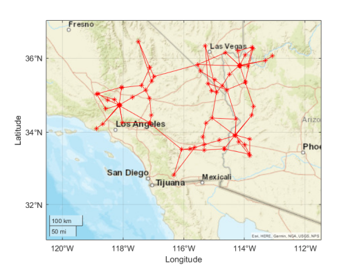
Figure 2: RTS GMLC test system with geographic information.

VII-B Parameter Value Settings

The parameters that are used in both the preventive and the corrective control formulations include the cost coefficients, i.e., $\bm{c}_{i}$, $\bm{c}_{i}^{r}$ and $\bm{c}_{i}^{\mathrm{voll}}$. The linear cost coefficient for each generator is directly used for $\bm{c}_{i}$. As for the ramping and value of lost load’s cost coefficients, they are set to $\bm{c}_{i}^{r}=10\%\times\bm{c}_{i}$ and $\bm{c}_{i}^{\mathrm{voll}}=10.0\times\max_{i}(c_{i})$. Note that $\bm{c}_{i}^{\mathrm{voll}}$ does not vary with $i$. In all the formulations presented in this paper, we do not explicitly differentiate up and down ramping for generators. Nevertheless, in all our implementations we treat up and down ramping differently, i.e., when a generator ramps up for an outage scenario $s$, we cost the excess generation using the cost $\bm{c}_{i}$ in addition to the ramping cost. We do not do so when a generator down ramps. This is because ramping generators up should be more expensive than ramping them down. To model this setup, one can change the objective coefficients and the formulations to treat up and down ramping differently for meeting an operator’s needs. Furthermore, in the PH algorithm, the primal and dual tolerances for the termination criteria are set to $10^{-3}$ and $10^{-2}$, respectively. Finally, the budget on the number of lines that can be controlled, namely $\bm{\beta}$, is set to 5 for all the computational experiments.

VII-C Computational Platform & Implementation Details

All the presented formulations were implemented in the Julia Programming language [34] using JuMP [35] as the mathematical programming layer. All computational experiments were run on a regular laptop equipped with Intel^® CPU @ 2.60 GHz and 12 GB of RAM. Furthermore, CPLEX, a commercial MILP solver, was used to solve all the optimization problems. The solver was set up to utilize up to 12 available threads. Finally, PowerModels.jl [36] was used to parse the RTS-GMLC’s MATPOWER case file. We now present the results of the various computational experiments that corroborate the utility of the formulations and the effectiveness of the algorithms to solve them.

VII-D Algorithm Performance

In this section, we first compare the computation time taken by the two versions of the PH algorithm where scenario sub-problems in Step 9 of Algorithm 1 are solved in (i) serial and (ii) in parallel. The two variants of the algorithm are used to solve both the preventive and corrective control formulations with a varying number of outage scenarios and two different loading factors from the set $\{1.0,1.05\}$.

Table I: Computation time in sec. (load scaling - $1.0$)

$|\mathcal{S}|$	preventive		corrective
	serial	parallel	serial	parallel
[late after line=

Table II: Computation time in sec. (load scaling - $1.05$)

$|\mathcal{S}|$	preventive		corrective
	serial	parallel	serial	parallel
[late after line=

Tables VII-D and VII-D show the computation time taken be the serial and parallel versions of the PH algorithm to solve the two formulations with the number of outage scenarios varying from $20$ to $200$ in steps of $20$. For these runs, the risk threshold in Algorithm 2 was set to the lowest possible, i.e., $\bm{R}=0$. This corresponds to the case where the outage scenarios are generated purely based on existing outage risk data in the literature [6] and that confidence in these outage scenarios is low. It is clear from the Tables VII-D and VII-D that the parallel versions of the PH algorithm is always preferable to the serial version and the former can provide a considerable computation time advantage. Another noticeable trend is that the computation time taken by both versions of the PH algorithm for solving the corrective control formulation is three to seven times faster than the preventive control formulation. This makes sense intuitively because in the corrective control formulation, the first stage has no binary variables and it is easier to obtain an implementable solution to be consistent (namely, $\vec{x}_{s}=\vec{x}$ for every $s\in\mathcal{S}$) in the case of continuous variables.

The next set of results in Table VII-D shows the number of iterations taken by the PH algorithm to converge to a solution that satisfies the termination criteria. From here on, in lieu of the previous results on computation time, we present the results only for the parallel version of the PH algorithm. The number of iterations taken by the PH algorithm to solve the corrective problem is always observed to be less than those for the preventive control problem. This is because the ease of obtaining a consistent implementable solution leads to faster convergence for the corrective problem.

Table III: Number of iterations for termination

$|\mathcal{S}|$	load scaling - 1.0		load scaling - 1.05
	preventive	corrective	preventive	corrective
[late after line=

VII-E Comparison of solutions

In this section, we compare the objective value obtained using the preventive and the corrective control formulations for a varying number of outage scenarios. As observed from Fig. 3 and Fig. 4, the objective values seem to stabilize and converge to a limit with an increasing number of scenarios. This will be true for any method that uses the sample-average approximation to solve the full two-stage stochastic optimization problem. We also remark that, in the base case with no outage scenarios, when the problem in Sec. III was solved to optimality, the total generation output was $85.5$ p.u. and no load-shedding was required.

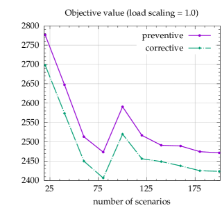
Figure 3: Objective value of the preventive and corrective control problems with varying number of scenarios for a load scaling of $1.0$

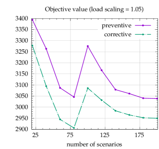
Figure 4: Objective value of the preventive and corrective control problems with varying number of scenarios for a load scaling of $1.05$

Another trend that is observed from Fig. 3 and Fig. 4 is that the objective value of the preventive control problem is always greater than the corrective control problem. Again, this is expected because the preventive control formulation aims to compute a single topology that is suitable for all the outage scenarios whereas the corrective control formulation seeks a different topology switching decision for each outage scenario. Thus, the corrective control formulation is able to produce a lower load shed for each damage scenario. The actual relative gap between the preventive and the corrective control formulations is shown in Table VII-E.

Table IV: Relative gap between the corrective and preventive formulations’ objective values (relative w.r.t preventive’s objective value)

$|\mathcal{S}|$	relative gap (%)
	load scaling - $1.0$	load scaling - $1.05$
[late after line=

Finally, Table VII-E shows the expected load that is shed over all the outage scenarios by the preventive and the corrective control formulations. These results indicate that if the operator is allowed to choose between a preventive or a corrective control formulation, it is always prudent to choose the corrective control formulation to minimize the load shed. Nevertheless, the topology switching policy obtained by the preventive control formulation is an easier one to implement from a practical standpoint as it can be done ahead of time and incurs no real-time changes.

Table V: Average load shed (in MW) over all the scenarios by the solutions of the preventive and corrective control formulations

$|\mathcal{S}|$	load scaling - 1.0		load scaling - 1.05
	preventive	corrective	preventive	corrective
[late after line=

VII-F Impact of Risk Threshold

All results presented thus far are on outage scenarios generated with $\bm{R}=0$, and keeping the value of $\bm{m}=4$ in Algorithm 2. The histogram in Fig. 5 shows the number of lines that are in at least $k$ outage scenarios. The histogram essentially indicates that when the risk is low, the failure probability or intuitively, the risk of line failure associated with the wildfire is spread over a large number of lines, i.e., $54$ lines in the RTS-GMLC network. Such a large number of lines with a non-zero failure probability indicates very low confidence in the outage scenarios, and hence preventive control has a much larger cost compared to corrective (scenario-wise) topology control.

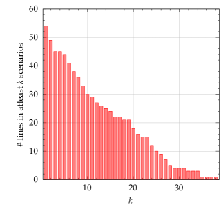
Figure 5: Histogram of the outage scenarios generated using $\bm{R}=0$. The outages are spread over $54$ lines, indicating low confidence on the outage scenarios. The first bar in the histogram indicates that $54$ unique lines are contained in at least $1$ outage scenario.

For comparing the solutions of the two formulations under high confidence of risk predictions, we generated a new set of $200$ scenarios where the risk of wildfire is restricted to $4$ lines. The histogram in this case is given by Fig. 6. The histogram can be understood as follows: there are at least $122$ scenarios where all the $4$ lines that have a non-zero risk of wildfire are contained in. This in turn translates to higher probability of these scenarios occurring, i.e., higher confidence in the outage scenarios. When the preventive and the corrective formulations were run on these scenarios, it was observed that the load shed obtained by the corrective and the preventive control formulations are relatively close to each other (see Table VII-F). This too is intuitive as the number of possible scenarios have a high order of overlap. As such, when the wildfire risk is known with high confidence, preventive control should be the right way forward as it is more easily implementable and does not lead to any significant loss in real-time optimal operation. For low-risk confidence, our method enables a quantification of the optimality loss in preventive (over real-time corrective control) and motivates the search for improved sampling and risk estimation strategies to mitigate them.

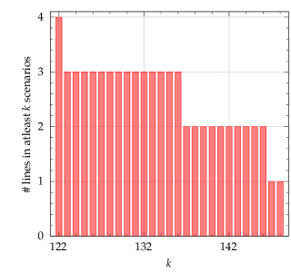
Figure 6: Histogram when the outage risk is spread over $4$ lines. Here, these four lines are present in at least $122$ out of the the $200$ outage scenarios that are generated. The histogram indicates high confidence on the outage scenarios.

Table VI: Average load shed (in MW) over all the scenarios for high confidence damage scenarios

load scaling - 1.0		load scaling - 1.05
preventive	corrective	preventive	corrective
[late after line=

VIII Conclusions

This paper considered the optimal topology control problem under line failures due to uncertain wildfires. To account for the uncertainty model of developing wildfires into the decision-making framework, we put forth a two-stage stochastic mixed-integer program. The optimization problem incorporates different scenarios of line outages due to the spreading wildfires, and seeks to obtain an optimal topology control strategy that provides the lowest operating costs. To enable line switching at different stages, we present both preventive and corrective control formulation, both of which can be efficiently solvable using a progressive hedging-based parallelizable solution strategy. Numerical studies on the practical RTS-GMLC system corroborate the performance of the proposed topology control algorithms for providing real-time wildfire mitigation solutions, and demonstrate that under lower risk confidence and threshold leads to a reduction in optimal operation of preventive (pre-wildfire) control policies over corrective (real-time wildfire) control policies.

This work leads to several directions of work. We are currently analyzing methods to ensure fair control policies under stochastic wildfires. Further improved sampling strategies for wildfire scenarios (including ones based on active/importance sampling) will lead to significant improvements over the current naive sampling strategy. Finally, linking the wildfire risk model with the grid control algorithm will ensure that the multiple sub-systems in grid-fire control are jointly optimized and not separately.

References

- [1] The National Interagency Fire Center. [Online]. Available: https://www.nifc.gov/fire-information
- [2] D. A. Z. Vazquez, F. Qiu, N. Fan, and K. Sharp, “Wildfire mitigation plans in power systems: A literature review,” IEEE Transactions on Power Systems, 2022.
- [3] “Effect of wildfires on transmission line reliability,” California Public Utilities Commission, Tech. Rep., 2008.
- [4] C. Coffrin, R. Bent, B. Tasseff, K. Sundar, and S. Backhaus, “Relaxations of ac maximal load delivery for severe contingency analysis,” IEEE Transactions on Power Systems, vol. 34, no. 2, pp. 1450–1458, 2018.
- [5] A. Kody, A. West, and D. K. Molzahn, “Sharing the load: Considering fairness in de-energization scheduling to mitigate wildfire ignition risk using rolling optimization,” arXiv preprint arXiv:2204.06543, 2022.
- [6] N. Rhodes, L. Ntaimo, and L. Roald, “Balancing wildfire risk and power outages through optimized power shut-offs,” IEEE Transactions on Power Systems, vol. 36, no. 4, pp. 3118–3128, 2020.
- [7] N. Rhodes and L. Roald, “Co-optimization of power line shutoff and restoration for electric grids under high wildfire ignition risk,” arXiv preprint arXiv:2204.02507, 2022.
- [8] A. Astudillo, B. Cui, and A. S. Zamzam, “Managing power systems-induced wildfire risks using optimal scheduled shutoffs,” in 2022 IEEE Power & Energy Society General Meeting (PESGM). IEEE, 2022, pp. 1–5.
- [9] A. Kody, R. Piansky, and D. K. Molzahn, “Optimizing transmission infrastructure investments to support line de-energization for mitigating wildfire ignition risk,” arXiv preprint arXiv:2203.10176, 2022.
- [10] S. Taylor and L. A. Roald, “A framework for risk assessment and optimal line upgrade selection to mitigate wildfire risk,” Electric Power Systems Research, vol. 213, p. 108592, 2022.
- [11] D. N. Trakas and N. D. Hatziargyriou, “Optimal distribution system operation for enhancing resilience against wildfires,” IEEE Transactions on Power Systems, vol. 33, no. 2, pp. 2260–2271, 2017.
- [12] M. Nazemi and P. Dehghanian, “Powering through wildfires: An integrated solution for enhanced safety and resilience in power grids,” IEEE Transactions on Industry Applications, vol. 58, no. 3, pp. 4192–4202, 2022.
- [13] M. Abdelmalak and M. Benidris, “Enhancing power system operational resilience against wildfires,” IEEE Transactions on Industry Applications, vol. 58, no. 2, pp. 1611–1621, 2022.
- [14] The California Department of Forestry and Fire Protection (CAL FIRE). [Online]. Available: https://www.fire.ca.gov/incidents
- [15] T. Tapia, Á. Lorca, D. Olivares, M. Negrete-Pincetic et al., “A robust decision-support method based on optimization and simulation for wildfire resilience in highly renewable power systems,” European Journal of Operational Research, vol. 294, no. 2, pp. 723–733, 2021.
- [16] J.-P. Watson and D. L. Woodruff, “Progressive hedging innovations for a class of stochastic mixed-integer resource allocation problems,” Computational Management Science, vol. 8, no. 4, p. 355, 2011.
- [17] B. Stott, J. Jardim, and O. Alsaç, “DC power flow revisited,” IEEE Transactions on Power Systems, vol. 24, no. 3, pp. 1290–1300, 2009.
- [18] E. B. Fisher, R. P. O’Neill, and M. C. Ferris, “Optimal transmission switching,” IEEE Trans. Power Systems, vol. 23, no. 3, pp. 1346–1355, 2008.
- [19] B. Kocuk, S. S. Dey, and X. A. Sun, “New formulation and strong MISOCP relaxations for AC optimal transmission switching problem,” IEEE Trans. Power Systems, vol. 32, no. 6, pp. 4161–4170, 2017.
- [20] E. A. Goldis, X. Li, M. C. Caramanis, A. M. Rudkevich, and P. A. Ruiz, “AC-based topology control algorithms (TCA)–A PJM historical data case study,” in 2015 48th Hawaii International Conference on System Sciences. IEEE, 2015, pp. 2516–2519.
- [21] A. Shapiro, “On complexity of multistage stochastic programs,” Operations Research Letters, vol. 34, no. 1, pp. 1–8, 2006.
- [22] R. Jiang, M. Zhang, G. Li, and Y. Guan, “Benders’ decomposition for the two-stage security constrained robust unit commitment problem,” in IIE Annual Conference. Proceedings. Institute of Industrial and Systems Engineers (IISE), 2012, p. 1.
- [23] R. Rahmaniani, T. G. Crainic, M. Gendreau, and W. Rei, “The benders decomposition algorithm: A literature review,” European Journal of Operational Research, vol. 259, no. 3, pp. 801–817, 2017.
- [24] C. C. Carøe and R. Schultz, “Dual decomposition in stochastic integer programming,” Operations Research Letters, vol. 24, no. 1-2, pp. 37–45, 1999.
- [25] J. R. Birge and F. Louveaux, Introduction to stochastic programming. Springer Science & Business Media, 2011.
- [26] R. T. Rockafellar and R. J.-B. Wets, “Scenarios and policy aggregation in optimization under uncertainty,” Mathematics of operations research, vol. 16, no. 1, pp. 119–147, 1991.
- [27] S. Atakan and S. Sen, “A progressive hedging based branch-and-bound algorithm for mixed-integer stochastic programs,” Computational Management Science, vol. 15, no. 3-4, pp. 501–540, 2018.
- [28] M. Biel and M. Johansson, “Efficient stochastic programming in julia,” INFORMS Journal on Computing, vol. 34, no. 4, pp. 1885–1902, 2022.
- [29] Y. Fan and C. Liu, “Solving stochastic transportation network protection problems using the progressive hedging-based method,” Networks and Spatial Economics, vol. 10, no. 2, pp. 193–208, 2010.
- [30] O. Listes and R. Dekker, “A scenario aggregation–based approach for determining a robust airline fleet composition for dynamic capacity allocation,” Transportation Science, vol. 39, no. 3, pp. 367–382, 2005.
- [31] A. Løkketangen and D. L. Woodruff, “Progressive hedging and tabu search applied to mixed integer (0, 1) multistage stochastic programming,” Journal of Heuristics, vol. 2, no. 2, pp. 111–128, 1996.
- [32] S. Zehtabian and F. Bastin, Penalty parameter update strategies in progressive hedging algorithm. Cirrelt Montreal, QC, Canada, 2016.
- [33] C. Barrows, A. Bloom, A. Ehlen, J. Ikäheimo, J. Jorgenson, D. Krishnamurthy, J. Lau, B. McBennett, M. O’Connell, E. Preston et al., “The ieee reliability test system: A proposed 2019 update,” IEEE Transactions on Power Systems, vol. 35, no. 1, pp. 119–127, 2019.
- [34] J. Bezanson, A. Edelman, S. Karpinski, and V. B. Shah, “Julia: A fresh approach to numerical computing,” SIAM review, vol. 59, no. 1, pp. 65–98, 2017.
- [35] I. Dunning, J. Huchette, and M. Lubin, “Jump: A modeling language for mathematical optimization,” SIAM Review, vol. 59, no. 2, pp. 295–320, 2017.
- [36] C. Coffrin, R. Bent, K. Sundar, Y. Ng, and M. Lubin, “Powermodels.jl: An open-source framework for exploring power flow formulations,” in 2018 Power Systems Computation Conference (PSCC), June 2018, pp. 1–8.