Adaptive mesh refinement for the
Landau–Lifshitz–Gilbert equation

Abstract.

We propose a new adaptive algorithm for the approximation of the Landau–Lifshitz–Gilbert equation via a higher-order tangent plane scheme. We show that the adaptive approximation satisfies an energy inequality and demonstrate numerically, that the adaptive algorithm outperforms uniform approaches.

1. Introduction

The Landau–Lifshitz–Gilbert equation (LLG) serves as an important practical tool and as a valid model of micromagnetic phenomena occurring in, e.g., magnetic sensors, recording heads, and magneto-resistive storage device [20, 25, 27]. Cutting edge examples include heat assisted magnetic recording [29], where lasers heat the magnetic recording material locally in order to speed up the writing process. Other developments, such as magneto-resistive memory and skyrmion based race-track memory focus on new ways to store data magnetically, see e.g., [18]. All of these applications have in common that the magnetic materials exhibit a strong locality (in time and space) of magnetic effects [28]: So called domain walls reveal a change of direction of the magnetization on small length scales. Similarly, temporal behavior is characterized by rapid changes (switching processes) followed by long relatively stable periods. Those effects render non-adaptive simulations tremendously inefficient (see [28] for early experiments and [17] for current applications) and classical methods based on uniform meshes often fail to reach meaningful accuracy even on the largest computers.

Even uniform time-stepping for the LLG equation is challenging. While weak convergence of the approximations was known since at least 2008 (see, e.g., [5, 10]), strong a priori convergence of uniform time-stepping schemes that obey physical energy bounds has first been proved recently in [15] and then extended to higher-order in [2]. The latter two works build on the tangent plane idea first introduced in [5] in order to remove the nonlinear solver required in [10]. This is achieved by solving for the time derivative of the magnetization $\partial_{t}\boldsymbol{m}$ instead of the magnetization itself. The constraint $|\boldsymbol{m}|=1$ translates to the orthogonality $\partial_{t}\boldsymbol{m}\cdot\boldsymbol{m}=0$ almost everywhere. In the discretization, this can only hold nodewise [5] or in an average sense [2]. As an attractive side effect, the discrete approximations still obey the physical energy decay. This is in contrast to other higher-order methods for LLG in [26, 24, 14] (without strong error analysis) and [19, 6] which do not satisfy discrete energy bounds.

While the higher-order convergence depends on certain regularity assumptions on the exact solution (see [16] for existence proofs of smooth solutions under a smallness condition on the initial data), it was shown in [2] that even without regularity beyond $H^{1}$ one can still get weak convergence (a consequence of the energy decay) and thus is at least as good as traditional first order schemes.

The aim of this work is to exploit the higher-order time-stepping schemes developed in [2] in order to obtain a heuristic estimate of the temporal approximation error. This will allow us to construct an adaptive time-stepping scheme for LLG. Combined with gradient recovery estimators for the spatial error, we derive a fully adaptive integrator for LLG. While a convergence proof seems out of reach for the moment, we demonstrate in several experiments the effectiveness of the method.

In Section 1.2 we introduce the initial value problem in its strong form. In Section 2 we present the spatial discretisation that is based on the standard higher order conforming finite element method and a Lagrangian setting to cope with the nonlinear constraint. For the time stepping, we use a collocation method based on the BDF-$k$ method (for $k=1,2$) with a predictor based on extrapolation. In the uniform setting this method has proved to converge with optimal rates in [2]. In Section 3 we formulate the BDF method with variable time steps. Furthermore we present approximations to higher order derivatives with finite differences in order to estimate the truncation error of a given order. This allows to suggest new time step sizes and likewise also orders. In Theorem 1 we show that under regularity requirements, restricted time step changes and a certain size of the damping term, the time-adaptive method satisfies an energy bound. In Sections 3 and 4 we formulate our adaptive method and conclude in Section 6 with some numerical experiments.

1.1. Notation

Let $\Omega\subset\mathbb{R}^{d}$, $d=2,3$, be a bounded domain with polygonally boundary. By $L^{2}(\Omega)$ we denote the usual Lebesgue spaces with scalar product $(v,w)_{\Omega}=\int_{\Omega}vw$ and norm $\|v\|_{L^{2}(\Omega)}=(v,v)_{\Omega}^{1/2}$. Vector valued functions are in $L^{2}(\Omega)^{d}$ if they are componentwise in $L^{2}(\Omega)$ and the scalar product is defined as $(\boldsymbol{v},\boldsymbol{w})_{\Omega}=\int_{\Omega}\boldsymbol{v}\cdot\boldsymbol{w}$. $H^{1}(\Omega)$ denotes the space of functions in $L^{2}(\Omega)$ with weak derivatives in $L^{2}(\Omega)$. A norm on $H^{1}(\Omega)$ is given by $(\|v\|_{L^{2}(\Omega)}^{2}+\|\boldsymbol{\nabla}v\|_{L^{2}(\Omega)}^{2})^{1/2}$.

In the following we work with vector valued functions $\boldsymbol{m}=[m_{1},m_{2},m_{3}]:(0,T)\times\Omega\to\mathbb{R}^{3}$. For convenience we use the notation $\boldsymbol{m}(t)=\boldsymbol{m}(t,\cdot):\Omega\to\mathbb{R}^{3}$. For $\boldsymbol{\nabla}\boldsymbol{m}$ we let $\|\boldsymbol{\nabla}\boldsymbol{m}\|_{L^{2}(\Omega)}^{2}=\int_{\Omega}\boldsymbol{\nabla}\boldsymbol{m}:\boldsymbol{\nabla}\boldsymbol{m}$, where ’$:$’ denotes the Frobenius product of two matrices. For vectors or tensors $|\cdot|$ denotes the euclidean norm or the Frobenius norm.

1.2. The Landau–Lifshitz–Gilbert-equation

The strong form of the LLG equations is to seek $\boldsymbol{m}:[0,T]\times\overline{\Omega}$ such that

(1.1) $$\alpha\partial_{t}\boldsymbol{m}+\boldsymbol{m}\times\partial_{t}\boldsymbol{m} =\boldsymbol{P}(\boldsymbol{m})\boldsymbol{H}_{\mathrm{eff}}(\boldsymbol{m})\qquad \text{on }(0,T)\times\Omega\,,$$

(1.2) $$\partial_{\boldsymbol{n}}\boldsymbol{m} =\boldsymbol{0} \text{on }(0,T)\times\partial\Omega\,,$$

(1.3) $$\boldsymbol{m}(0) =\boldsymbol{m}^{0} \text{in }\Omega\,,$$

with a given vector field $\boldsymbol{m}^{0}:\Omega\to\mathbb{R}^{3}$ of unit length, i. e., $|\boldsymbol{m}^{0}|=1$. $\boldsymbol{P}$ is the projection operator $\boldsymbol{P}(\boldsymbol{m})=\boldsymbol{\mathit{Id}}-\frac{\boldsymbol{m}\,\raise 2.0pt\hbox{${}_{\otimes}$}\boldsymbol{m}}{|\boldsymbol{m}|^{2}}$ for $\boldsymbol{m}\not=\boldsymbol{0}$. In this paper we let the effective field be given as

(1.4) $$\boldsymbol{H}_{\text{eff}}(\boldsymbol{m})=C_{\mathrm{e}}\Delta\boldsymbol{m}+\boldsymbol{H}_{\mathrm{ext}}\,.$$

Formally, we can derive from (1.1), by multiplying with $\boldsymbol{m}$, that $\partial_{t}|\boldsymbol{m}(t)|^{2}=0$, hence $|\boldsymbol{m}(t)|=|\boldsymbol{m}^{0}|=1$. Multiplying with $\partial_{t}\boldsymbol{m}$ and integrating will lead to the energy inequality

(1.5) $$\mathcal{E}(t) =C_{\mathrm{e}}\|\boldsymbol{\nabla}\boldsymbol{m}(t)\|_{L^{2}(\Omega)}^{2}+\frac{\alpha}{2}\int_{0}^{t}\|\partial_{t}\boldsymbol{m}(s)\|_{L^{2}(\Omega)}^{2}\,\mathrm{d}s$$

$$\leq C_{\mathrm{e}}\|\boldsymbol{\nabla}\boldsymbol{m}(0)\|_{L^{2}(\Omega)}^{2}+\frac{1}{2\alpha}\int_{0}^{t}\|\boldsymbol{H}_{\mathrm{ext}}(s)\|_{L^{2}(\Omega)}^{2}\,\mathrm{d}s$$

for all $t\in[0,T]$.

2. Discretisation of the Landau–Lifshitz–Gilbert-equation

2.1. Weak formulation

The derivation of a weak form can be simplified if one uses test functions $\boldsymbol{\varphi}\in C^{\infty}(\Omega)^{3}$ with $\boldsymbol{m}(t)\cdot\boldsymbol{\varphi}=0$ at time $t>0$, since it will allow us later to replace $\boldsymbol{P}(\boldsymbol{m})$ in (1.1) by $\boldsymbol{\mathit{Id}}$. Thus we define the solution dependent constraint space by

$$\mathbb{T}(\boldsymbol{m}(t))=\big{\{}\boldsymbol{\varphi}\in H^{1}(\Omega)^{3}\mid\boldsymbol{m}(t)\cdot\boldsymbol{\varphi}=0\big{\}}\,.$$

For ease of notation we will omit the argument $t$ in the subsequel and arrive formally at the following weak equation for $\boldsymbol{m}$

$$\alpha(\partial_{t}\boldsymbol{m},\boldsymbol{\varphi})_{\Omega}+(\boldsymbol{m}\times\partial_{t}\boldsymbol{m},\boldsymbol{\varphi})_{\Omega}+C_{\mathrm{e}}(\boldsymbol{\nabla}\boldsymbol{m},\boldsymbol{\nabla}\boldsymbol{\varphi})_{\Omega}=(\boldsymbol{H}_{\mathrm{ext}},\boldsymbol{\varphi})_{\Omega}\qquad\text{for all }\boldsymbol{\varphi}\in\mathbb{T}(\boldsymbol{m})\,.$$

Existence of weak solutions $\boldsymbol{m}\in H^{1}(\Omega)^{3}$ is well-known (see, e.g., [27]) and follows with a standard Galerkin–Fadeo approximation and compactness arguments. Uniqueness of weak solutions is open in general and there are non-uniqueness results for the related harmonic map heat flow [12]. Note that in case one of the weak solutions is also a strong solution, we have uniqueness [13]. In terms of regularity, it is suspected that even smooth initial conditions can lead to blow up of $\nabla\boldsymbol{m}$ in $L^{\infty}(\Omega)^{3,3}$ in finite time, however, no proof is known. For LLG on smooth bounded domains with Neumann boundary conditions, smooth initial data close to constants lead to arbitrarily smooth solutions [16].

2.2. Spatial discretisation

Since $\Omega$ is assumed to be polygonally bounded, we let $\mathcal{K}_{h}$ be a regular triangulation such that $\overline{\Omega}=\bigcup\{K\in\mathcal{K}_{h}\}$. On $\mathcal{K}_{h}$ we consider the finite element space $W_{h}\subset H^{1}(\Omega)$ of constant degree $p\geq 1$. For vector fields we then use $\boldsymbol{V}_{h}=W_{h}^{3}\subset H^{1}(\Omega)^{3}$. It looks quite natural to correspondingly define the discrete constraint space by

$$\mathbb{T}_{h}^{\mathrm{s}}(\boldsymbol{m}_{h})=\big{\{}\boldsymbol{\varphi}_{h}\in\boldsymbol{V}_{h}\mid\boldsymbol{m}_{h}\cdot\boldsymbol{\varphi}_{h}=0\text{ at every node}\big{\}}$$

for some $\boldsymbol{m}_{h}\in H^{1}(\Omega)^{3}$. Since this choice leads to problems with higher order convergence [2, Rem. 2.2] the method for which this could be achieved in [2] is based on the weaker constraint space

$$\mathbb{T}_{h}(\boldsymbol{m}_{h})=\mathbb{T}_{h}^{\mathrm{w}}(\boldsymbol{m}_{h})=\big{\{}\boldsymbol{\varphi}_{h}\in\boldsymbol{V}_{h}\mid(\boldsymbol{m}_{h}\cdot\boldsymbol{\varphi}_{h},\psi_{h})_{\Omega}=0\text{ for all }\psi_{h}\in W_{h}\big{\}}\,.$$

It is then straightforward to define the semi-discrete solution $\boldsymbol{m}_{h}:[0,T]\to\boldsymbol{V}_{h}$ by

$$\alpha(\partial_{t}\boldsymbol{m}_{h},\boldsymbol{\varphi}_{h})_{\Omega}+(\boldsymbol{m}_{h}\times\partial_{t}\boldsymbol{m}_{h},\boldsymbol{\varphi}_{h})_{\Omega}+C_{\mathrm{e}}(\boldsymbol{\nabla}\boldsymbol{m}_{h},\boldsymbol{\nabla}\boldsymbol{\varphi}_{h})_{\Omega} =(\boldsymbol{H}_{\mathrm{ext}},\boldsymbol{\varphi}_{h})_{\Omega}$$

$$\qquad\text{for all }\boldsymbol{\varphi}_{h}\in\mathbb{T}_{h}(\boldsymbol{m}_{h})\,.$$

2.3. Temporal discretisation

We complete the discretisation by defining a time-stepping method. For this we let $0=t_{0}<\dots<t_{N_{T}}=T$ be a decomposition of the interval $[0,T]$. The finite element space at a time $t_{n}\in[0,T]$ may change due to regular refinement (and derefinement) of the preceding one and is denoted by $\boldsymbol{V}_{h}^{n}$. We want to set up an equation for the approximation $\boldsymbol{m}^{n}\approx\boldsymbol{m}(t_{n})$ at time $t_{n}$. Further we introduce the unknown $\boldsymbol{v}^{n}\approx\partial_{t}\boldsymbol{m}(t_{n})$ and assume that we can impose a relation between $\boldsymbol{v}_{h}^{n}$ and $\boldsymbol{m}_{h}^{n-j}$ for a set of indices $j\geq 0$. For example, if we assume a linear time-dependence of $\boldsymbol{m}_{h}$, we can state $\boldsymbol{m}_{h}^{n}=\boldsymbol{m}_{h}^{n-1}+\tau_{n}\boldsymbol{v}_{h}^{n}$. Thus the resulting equation

$$\alpha(\boldsymbol{v}_{h}^{n},\boldsymbol{\varphi}_{h})_{\Omega}+(\boldsymbol{m}_{h}^{n}\times\boldsymbol{v}_{h}^{n},\boldsymbol{\varphi}_{h})_{\Omega}+C_{\mathrm{e}}(\boldsymbol{\nabla}\boldsymbol{m}_{h}^{n},\boldsymbol{\nabla}\boldsymbol{\varphi}_{h})_{\Omega}=(\boldsymbol{H}_{\mathrm{ext}}^{n},\boldsymbol{\varphi}_{h})_{\Omega}\qquad\text{for all }\boldsymbol{\varphi}_{h}\in\mathbb{T}_{h}(\boldsymbol{m}_{h}^{n})$$

can be seen as a nonlinear equation for $\boldsymbol{v}_{h}^{n}$ from which $\boldsymbol{m}_{h}^{n}$ could then easily be obtained. However, we have to note that the test space also depends on $\boldsymbol{v}_{h}^{n}$. This approach is called tangent plane scheme [23].

The following linearisation has turned out to be useful: construct an approximation (or predictor) $\widehat{\boldsymbol{m}}_{h}^{n}$ to $\boldsymbol{m}_{h}^{n}$ and then define $\boldsymbol{m}_{h}^{n}$ by

$$\alpha(\boldsymbol{v}_{h}^{n},\boldsymbol{\varphi}_{h})_{\Omega}+(\widehat{\boldsymbol{m}}_{h}^{n}\times\boldsymbol{v}_{h}^{n},\boldsymbol{\varphi}_{h})_{\Omega}+C_{\mathrm{e}}(\boldsymbol{\nabla}\boldsymbol{m}_{h}^{n},\boldsymbol{\nabla}\boldsymbol{\varphi}_{h})_{\Omega}=(\boldsymbol{H}_{\mathrm{ext}}^{n},\boldsymbol{\varphi}_{h})_{\Omega}\quad\text{for all }\boldsymbol{\varphi}_{h}\in\mathbb{T}_{h}(\widehat{\boldsymbol{m}}_{h}^{n})$$

which is now a linear problem for $\boldsymbol{v}_{h}^{n}$. There is still the problem to cope with the constraint, for example, one might construct a local basis [2, Sect. 2.2]. Here we will add the constraint as a separate weak equation. Thus we introduce the Lagrange variable $\lambda_{h}^{n}\in W_{h}$ and state the saddle point problem

(2.1) $$\alpha(\boldsymbol{v}_{h}^{n},\boldsymbol{\varphi}_{h})_{\Omega}+(\widehat{\boldsymbol{m}}_{h}^{n}\times\boldsymbol{v}_{h}^{n},\boldsymbol{\varphi}_{h})_{\Omega}+C_{\mathrm{e}}(\boldsymbol{\nabla}\boldsymbol{m}_{h}^{n},\boldsymbol{\nabla}\boldsymbol{\varphi}_{h})_{\Omega}$$

$${}+(\widehat{\boldsymbol{m}}_{h}^{n}\cdot\boldsymbol{\varphi}_{h},\lambda_{h}^{n})_{\Omega} =(\boldsymbol{H}_{\mathrm{ext}}^{n},\boldsymbol{\varphi}_{h})_{\Omega} \qquad\text{for all }\boldsymbol{\varphi}_{h}\in\boldsymbol{V}_{h}^{n},$$

$$(\widehat{\boldsymbol{m}}_{h}^{n}\cdot\boldsymbol{v}_{h}^{n},\psi_{h})_{\Omega} =0 \qquad\text{for all }\psi_{h}\in W_{h}^{n}\,.$$

Note that the analysis of [2] is based on this formulation. It is straightforward to show that the discrete formulation is well-posed and leads to a unique discrete solution $\boldsymbol{v}_{h}^{n}$.

2.4. BDF time stepping

For the time stepping we now use especially the BDF (backward differencing) scheme of order $k\in\mathbb{N}$. It provides a general relation

(2.2) $$\xi_{k}\boldsymbol{m}_{h}^{n}=\widetilde{\boldsymbol{\Phi}}_{k}(\boldsymbol{m}_{h}^{n-1},\dots,\boldsymbol{m}_{h}^{n-k})+\tau_{n}\boldsymbol{v}_{h}^{n}$$

for $n\geq k$ and an affine linear mapping $\widetilde{\boldsymbol{\Phi}}_{k}:(\mathbb{R}^{3})^{k}\to\mathbb{R}^{3}$. The case $k=1$ has been given as an example in the previous Section  2.3, more details will be provided in Section 3. We insert this relation into (2.1) and get the following linear equation for $\boldsymbol{v}_{h}^{n}$

$$\alpha(\boldsymbol{v}_{h}^{n},\boldsymbol{\varphi}_{h})_{\Omega}+(\widehat{\boldsymbol{m}}_{h}^{n}\times\boldsymbol{v}_{h}^{n},\boldsymbol{\varphi}_{h})_{\Omega}+\beta_{k}\tau_{n}(\boldsymbol{\nabla}\boldsymbol{v}_{h}^{n},\boldsymbol{\nabla}\boldsymbol{\varphi}_{h})_{\Omega}$$

(2.3) $${}+(\widehat{\boldsymbol{m}}_{h}^{n}\cdot\boldsymbol{\varphi}_{h},\lambda_{h}^{n})_{\Omega} =\langle\boldsymbol{f}^{n}\,,\,\boldsymbol{\varphi}_{h}\rangle_{\Omega} \qquad\text{for all }\boldsymbol{\varphi}_{h}\in\boldsymbol{V}_{h}^{n},$$

$$(\widehat{\boldsymbol{m}}_{h}^{n}\cdot\boldsymbol{v}_{h}^{n},\psi_{h})_{\Omega} =0 \qquad\text{for all }\psi_{h}\in W_{h}^{n}\,,$$

with $\beta_{k}=C_{\mathrm{e}}/\xi_{k}$ and the new right hand side

(2.4) $$\langle\boldsymbol{f}^{n}\,,\,\boldsymbol{\varphi}_{h}\rangle_{\Omega}:=(\boldsymbol{H}_{\mathrm{ext}}^{n},\boldsymbol{\varphi}_{h})_{\Omega}-\beta_{k}(\boldsymbol{\nabla}\widetilde{\boldsymbol{\Phi}}_{k}(\boldsymbol{m}_{h}^{n-1},\dots,\boldsymbol{m}_{h}^{n-k}),\boldsymbol{\nabla}\boldsymbol{\varphi}_{h})_{\Omega}\,.$$

$\boldsymbol{m}_{h}^{n}$ is then defined by (2.2). Note that a discrete solution $\boldsymbol{v}_{h}^{n}$ exists since the form is coercive on $\mathbb{T}_{h}(\widehat{\boldsymbol{m}}_{h}^{n})$.

As an example for a predictor $\widehat{\boldsymbol{m}}_{h}^{n}$ one can take extrapolation of order $k-1$, i.e., seek the unique polynomial $\boldsymbol{q}\in\mathbb{P}_{k-1}$ with $\boldsymbol{q}(t_{n-1-j})=\boldsymbol{m}_{h}^{n-1-j}$ for $j=0,\dots,k-1$, and set $\widehat{\boldsymbol{m}}_{h}^{n}=\boldsymbol{q}(t_{n})/|\boldsymbol{q}(t_{n})|$. This problem has been analyzed in [2] and it was possible to prove, for uniform step size $\tau$, unconditional convergence in time up to order two [2, Thm. 3.1] and convergence up to order five in $h$ with some restrictions on $\alpha$ [2, Thm. 3.4].

2.5. The uniform discretisation

We consider a fixed (almost) uniform mesh of meshsize $h$ with a finite element method of polynomial order $p$ and in time BDF-$k$ for $k=1,\dots,5$. We will make regularity requirements for weak solutions as in [2, (3.2)]

(2.5) $$\begin{split}\boldsymbol{m}\in&\ C^{k+1}([0,T],L^{\infty}(\Omega)^{3})\cap C^{1}([0,T],W^{p+1,\infty}(\Omega)^{3})\,,\\ &\Delta\boldsymbol{m}+\boldsymbol{H}_{\mathrm{ext}}\in C^{0}([0,T],W^{p+1,\infty}(\Omega)^{3})\,.\end{split}$$

Then it has been proved in [2] that for sufficiently small $\tau$ and $h$ the discrete solutions exist and it holds

(2.6) $$\|\boldsymbol{\nabla}(\boldsymbol{m}(t_{n})-\boldsymbol{m}_{h}^{n})\|_{\Omega}\leq C(\tau^{k}+h^{p})$$

for $t_{n}=n\tau\leq T$. In case $k\in\{1,2\}$ one needs the additional condition $\tau\leq C\sqrt{h}$ [2, Thm. 3.1], while in case $k\in\{3,4,5\}$ one requires $p\geq 2$, $\tau\leq Ch$, and $\alpha\geq\alpha_{k}>0$ for some numbers $\alpha_{k}$ [2, Thm. 3.4].

3. Adaptivity in Time

3.1. The variable step BDF method

To describe the BDF method of order $k$ for $k\in\mathbb{N}$ we find it convenient to work on the grid

$$[0,t_{1},\dots,t_{k}]=[0,\tau_{1},\tau_{1}+\tau_{2},\tau_{1}+\dots+\tau_{k}]$$

for positive step sizes $\tau_{j}$, $j=1,\dots,k$. This can afterwards be translated to a mesh of the form $t_{n-k},\dots,t_{n}]$ (for $n\geq k$) by index shift. We will use abbreviations

$$\tau_{12}=\tau_{1}+\tau_{2},\ \tau_{23}=\tau_{2}+\tau_{3},\ \tau_{122}=\tau_{1}+2\tau_{2},\ \dots$$

and let $\tau=\max\{\tau_{1},\dots,\tau_{k}\}$. The definition of a variable step BDF method to solve the ordinary differential equation (ODE) $\boldsymbol{y}^{\prime}=\boldsymbol{F}(t,\boldsymbol{y})$, $\boldsymbol{y}:[0,T]\to\mathbb{R}^{N}$, $\boldsymbol{F}:[0,T]\times\mathbb{R}^{N}\to\mathbb{R}^{N}$, is as follows: Given $\{\boldsymbol{y}^{j}\}_{j=0}^{k-1}$, determine $\boldsymbol{y}^{k}$ (approximating $\boldsymbol{y}(t_{k})$) such that there is a polynomial $\boldsymbol{q}\in\mathbb{P}_{k}^{m}$ with

$$\boldsymbol{q}(t_{j})=\boldsymbol{y}^{j},\ j=0,\dots,k-1,\qquad\boldsymbol{q}^{\prime}(t_{k})=\boldsymbol{F}(t_{k},\boldsymbol{y}^{k})\,.$$

This leads to a nonlinear equation of the form

(3.1) $$\boldsymbol{\Phi}_{k}(\boldsymbol{y})=\xi_{k}\boldsymbol{y}-\widetilde{\boldsymbol{\Phi}}_{k}(\boldsymbol{y}^{k-1},\dots,\boldsymbol{y}^{0})-\tau_{k}\boldsymbol{F}(t_{k},\boldsymbol{y})=\boldsymbol{0}\,,$$

with $\xi_{k}>0$, to determine $\boldsymbol{y}^{k}$. For $k=1,2,3$ we obtain the explicit formulae

(3.2) $$\boldsymbol{\Phi}_{1}(\boldsymbol{y}) =\boldsymbol{y}-\boldsymbol{y}^{0}-\tau_{1}\boldsymbol{F}(t_{1},\boldsymbol{y})\,,$$

(3.3) $$\boldsymbol{\Phi}_{2}(\boldsymbol{y}) =\frac{\tau_{122}}{\tau_{12}}\boldsymbol{y}-\frac{\tau_{12}}{\tau_{1}}\boldsymbol{y}^{1}+\frac{\tau_{2}^{2}}{\tau_{1}\tau_{12}}\boldsymbol{y}^{0}-\tau_{2}\boldsymbol{F}(t_{2},\boldsymbol{y})\,.$$

If we compare this to (2.2), we can get the values for $\xi_{k}$ and expressions for $\widetilde{\boldsymbol{\Phi}}_{k}(\boldsymbol{y}^{k-1},\dots,\boldsymbol{y}^{0})$. These formulas agree with those in the case of constant $\tau$ [22, Ch. V]. Recall that for $k=1$ we get the implicit Euler method.

We will, in the provided notation and for later use, formulate consistent approximations for second and third order derivatives

(3.4) $$\partial_{\tau}^{2}\boldsymbol{y}(t_{2}) =2\Big{(}\frac{1}{\tau_{12}\tau_{2}}\boldsymbol{y}_{2}-\frac{1}{\tau_{1}\tau_{2}}\boldsymbol{y}_{1}+\frac{1}{\tau_{1}\tau_{12}}\boldsymbol{y}_{0}\Big{)}\,,$$

(3.5) $$\partial_{\tau}^{3}\boldsymbol{y}(t_{3}) =6\Big{(}\frac{1}{\tau_{123}\tau_{23}\tau_{3}}\boldsymbol{y}_{3}-\frac{1}{\tau_{12}\tau_{2}\tau_{3}}\boldsymbol{y}_{2}+\frac{1}{\tau_{1}\tau_{2}\tau_{23}}\boldsymbol{y}_{1}-\frac{1}{\tau_{1}\tau_{12}\tau_{123}}\boldsymbol{y}_{0}\Big{)}\,.$$

3.2. Time step selection

In the beginning we will always start with the first order method, i.e., the implicit Euler method ($\boldsymbol{\Phi}_{1}$). Since the local truncation error LTE at a time $t$ is known to be $1/2\,|\boldsymbol{y}^{\prime\prime}(t)|\tau^{2}$, we suggest as a next time step

(3.6) $$\tau_{n}^{[1]}:=\Big{(}\frac{2\,\mathrm{TOL}}{|\boldsymbol{y}^{\prime\prime}(t_{n})|}\Big{)}^{1/2}\,,$$

with the idea to get $\mathrm{TOL}\geq\text{LTE}\approx|\boldsymbol{y}^{\prime\prime}(t_{n})|\tau_{n}^{2}$. In order to evaluate this we use

(3.7) $$\boldsymbol{y}^{\prime\prime}(t_{n})=\partial_{t}\boldsymbol{F}(t_{n},\boldsymbol{y}(t_{n}))+\partial_{\boldsymbol{y}}\boldsymbol{F}(t_{n},\boldsymbol{y}(t_{n}))\boldsymbol{F}(t_{n},\boldsymbol{y}(t_{n}))\,,$$

but alternatively, we may use the finite difference approximation $\partial_{\tau}^{2}\boldsymbol{y}(t_{n})$ (3.4) for $n\geq 2$.

The next order method is given by $\boldsymbol{\Phi}_{2}$ and the truncation error in the uniform case is known to be $1/3\,|\boldsymbol{y}^{\prime\prime\prime}(t)|\tau^{3}$. In the case of variable step sizes we use Taylor expansion of $\boldsymbol{\Phi}_{2}(\boldsymbol{y}(t))$ in $t_{n}$ and get the local truncation error $1/6\,\tau_{n-1,n}\tau_{n}^{2}\,|\boldsymbol{y}^{\prime\prime\prime}(t_{n})|$ and from this the idea to let

(3.8) $$\tau_{n}^{[2]}:=\Big{(}\frac{6\,\mathrm{TOL}}{\tau_{n-1,n}|\boldsymbol{y}^{\prime\prime\prime}(t_{n})|}\Big{)}^{1/2}\,.$$

At this point we will relay on the finite difference approximation $\partial_{\tau}^{3}\boldsymbol{y}(t_{n})$ (3.5) for $n\geq 3$.

Every time step choice will be subject to a restriction compared to the previous step in the form

$$\tau_{n}^{*} =\max\big{\{}\tau_{n}^{[k]}\mid k_{\min}\leq k\leq k_{\max}\big{\}}=\tau_{n}^{[k_{n}^{*}]}\,,$$

$$\tau_{n+1} =\max\big{\{}\tau_{\min},\frac{1}{2}\tau_{n},\min\{\tau_{n}^{*},\sqrt{2}\,\tau_{n},\tau_{\max}\}\big{\}}\,,$$

where $k_{\min}\leq k_{\max}\in\mathbb{N}$ determine the set of admissible orders and $k_{n}^{*}$ notes which order provides the maximal step size. $\tau_{\min}$ and $\tau_{\max}$ are prescribed lower and upper bounds for the time step size. Note that values $|\boldsymbol{y}^{\prime\prime}(t_{n})|,|\boldsymbol{y}^{\prime\prime\prime}(t_{n})|$ close or equal to $0$ are of no harm since we have set a value $\tau_{\max}$. If we also allow order selection, we will choose $k_{n+1}=\max\{k_{\min},k_{n}-1,\min\{k_{n}^{*},k_{n}+1,k_{\max}\}\}$. In case the nonlinear equations are solved with Newton’s method, we might prevent the number of steps to be beyond, say, $4$ and thus prohibit enlargement of $\tau_{n}$ in case this number is reached.

3.3. Application to LLG

We iteratively solve (2.3), starting from a normalized initial condition $\boldsymbol{m}_{h}^{0}$ that approximates $\boldsymbol{m}^{0}$. The BDF-2 method with variable stepsize is then defined by Sections 2, 3.1, and 3.2 in the case $k=2$, taking $L^{2}(\Omega)$-norms for the difference quotients in time. Then we use extrapolation of order $k-1$ to define the prediction $\widehat{\boldsymbol{m}}_{h}^{n}$ [2, (2.1)]. An important statement about the uniform BDF-2 method for LLG is the validity of the energy inequality [2, Prop. 3.1]. We can derive a corresponding result for BDF-2 with variable stepsize under the condition that the coarsening factor is limited, and $\alpha$ has a positive lower bound.

Theorem 1 (Energy inequality for orders $k=1,2$).

Consider the discretization (2.3) of the LLG equation (1.1) for $k\in\{1,2\}$ with finite elements of polynomial degree $p\geq 1$. Let, for $k=2$, the time steps fulfill $\tau_{n}/\tau_{n-1}\leq\kappa_{0}\leq\sqrt{2}+1$ and $\alpha\geq\alpha_{2}>0$ for some $\alpha_{2}$ that depends on $\kappa_{0}$. Then, the numerical solution satisfies the following discrete energy inequality: for $n>k$ it holds

$$\gamma_{k}^{-}\|\boldsymbol{\nabla}\boldsymbol{m}_{h}^{n}\|_{L^{2}(\Omega)}^{2}+\frac{1}{2}\alpha\sum_{j=k}^{n}\tau_{j}\|\dot{\boldsymbol{m}}_{h}^{j}\|_{L^{2}(\Omega)}^{2}\leq\gamma_{k}^{+}\sum_{i=0}^{k-1}\|\boldsymbol{\nabla}\boldsymbol{m}_{h}^{i}\|_{L^{2}(\Omega)}^{2}+\frac{1}{2\alpha}\sum_{j=k}^{n}\tau_{j}\|\boldsymbol{H}_{\mathrm{ext}}(t_{j})\|_{L^{2}(\Omega)}^{2}$$

for some positive constants $\gamma_{k}^{-},\gamma_{k}^{+}$ when the solution fulfills the regularity requirements (2.5).

Proof.

We first note that the BDF-formula provides coefficients $\delta_{j}$, $j=0,\dots,k$, such that

$$\tau_{n}\dot{\boldsymbol{m}}_{h}^{n}=\sum_{j=0}^{k}\delta_{j}\boldsymbol{m}_{h}^{n-j}\,,$$

see Section 3.1. As in [2] we choose $\eta>0$, write down the weak equation for $\boldsymbol{m}_{h}^{n}-\eta\boldsymbol{m}_{h}^{n-1}$ and test it with $\dot{\boldsymbol{m}}_{h}^{n}$. The main point is a lower bound for $(\boldsymbol{\nabla}(\boldsymbol{m}_{h}^{n}-\eta\boldsymbol{m}_{h}^{n-1}),\boldsymbol{\nabla}\dot{\boldsymbol{m}}_{h}^{n})_{\Omega}$. If we let

$$\delta(s):=\sum_{i=0}^{k}\delta_{i}s^{i}\,,$$

and if we can show that $\operatorname{Re}(\delta(s)/(1-\eta s))>0$ for all complex $s$ with $|s|<1$, then [2, Lemma A.2] guarantees the existence of the required constants. The case $k=1$ is clear. In the case $k=2$, we let $\tau_{n}=\kappa\tau$ and $\tau_{n-1}=\tau$ for some $\kappa>0$. From (3.3) we get

$$\delta_{0}=\frac{1+2\kappa}{1+\kappa}\,,\quad\delta_{1}=-(1+\kappa)\,,\quad\delta_{2}=\frac{\kappa^{2}}{1+\kappa}\,.$$

We see immediately that $\delta$ has two zeros $s_{1}=1$ and $s_{2}=(1+2\kappa)/\kappa^{2}>1$ as long as $\kappa<1+\sqrt{2}$. Thus, we have

$$\frac{\delta(s)}{1-\eta s}=\frac{\delta_{2}(s-1)(s-s_{2})}{1-\eta s}=\frac{\delta_{2}(s-1)(s-s_{2})(1-\eta\overline{s})}{|1-\eta s|}\,.$$

Clearly, the choice $\eta=1/s_{2}$ would suffice to ensure $\operatorname{Re}(\delta(s)/(1-\eta s))>0$ for $|s|<1$. However, we obtain a sharper bound by resolving the inequality

$$\operatorname{Re}\big{(}(s-1)(s-s_{2})(1-\eta\overline{s})\big{)}>0\qquad\text{for }|s|<1\,.$$

Considering the edge case $|s|=1$ leads to the following quadratic inequality for the real part $s_{r}$ of $s$ (the cubic terms cancel)

$$2s_{r}^{2}-(1+\eta)(1+s_{2})s_{r}+(1+\eta)s_{2}+\eta-1>0\qquad\text{for all }-1<s_{r}<1\,.$$

For given $0<\kappa<1+\sqrt{2}$ this can be fulfilled if

$$\eta>\frac{3-s_{2}}{s_{2}+1}=\frac{3\kappa^{2}-2\kappa-1}{\kappa^{2}+2\kappa+1}\,.$$

For $\kappa\leq 1$ we can take $\eta=0$ and for $\kappa\in(1,1+\sqrt{2})$ we find $\eta<1$. Note that this bound dates back to [21] but was proved with a different method.

Let us first take for simplicity $\boldsymbol{H}_{\mathrm{ext}}^{n}=\boldsymbol{0}$. We proceed in recalling the weak equations for $\boldsymbol{v}_{h}^{n}$ and $\boldsymbol{v}_{h}^{n-1}$, for $n\geq 2$,

$$\alpha(\boldsymbol{v}_{h}^{n},\boldsymbol{\varphi}_{h})_{\Omega}+(\widehat{\boldsymbol{m}}_{h}^{n}\times\boldsymbol{v}_{h}^{n},\boldsymbol{\varphi}_{h})_{\Omega}+C_{\mathrm{e}}(\boldsymbol{\nabla}\boldsymbol{m}_{h}^{n},\boldsymbol{\nabla}\boldsymbol{\varphi}_{h})_{\Omega}=0\quad\text{for all }\boldsymbol{\varphi}_{h}\in\mathbb{T}_{h}(\widehat{\boldsymbol{m}}_{h}^{n})\,,$$

$$\alpha(\boldsymbol{v}_{h}^{n-1},\boldsymbol{\varphi}_{h})_{\Omega}+(\widehat{\boldsymbol{m}}_{h}^{n-1}\times\boldsymbol{v}_{h}^{n-1},\boldsymbol{\varphi}_{h})_{\Omega}+C_{\mathrm{e}}(\boldsymbol{\nabla}\boldsymbol{m}_{h}^{n-1},\boldsymbol{\nabla}\boldsymbol{\varphi}_{h})_{\Omega}=0\quad\text{for all }\boldsymbol{\varphi}_{h}\in\mathbb{T}_{h}(\widehat{\boldsymbol{m}}_{h}^{n-1})\,.$$

In order to derive an equation for $\boldsymbol{v}_{h}^{n}-\eta\boldsymbol{v}_{h}^{n-1}$ we use the test function $\boldsymbol{v}_{h}^{n}\in\mathbb{T}_{h}(\widehat{\boldsymbol{m}}_{h}^{n})$ in the first equation and $\widehat{\boldsymbol{P}}_{h}^{n-1}\boldsymbol{v}_{h}^{n}$ with $\widehat{\boldsymbol{P}}_{h}^{n-1}:=\boldsymbol{P}(\widehat{\boldsymbol{m}}_{h}^{n-1})\in\mathbb{T}_{h}(\widehat{\boldsymbol{m}}_{h}^{n-1})$ in the second equation. This latter term will be written in the form $\widehat{\boldsymbol{P}}_{h}^{n-1}\boldsymbol{v}_{h}^{n}=\boldsymbol{v}_{h}^{n}-(\widehat{\boldsymbol{P}}_{h}^{n}-\widehat{\boldsymbol{P}}_{h}^{n-1})\boldsymbol{v}_{h}^{n}=\boldsymbol{v}_{h}^{n}-\boldsymbol{p}_{h}^{n}$. Insertion of these test functions results in

$$\alpha(\boldsymbol{v}_{h}^{n},\boldsymbol{v}_{h}^{n})_{\Omega}+C_{\mathrm{e}}(\boldsymbol{\nabla}\boldsymbol{m}_{h}^{n},\boldsymbol{\nabla}\boldsymbol{v}_{h}^{n})_{\Omega}=0\,,$$

$$\alpha(\boldsymbol{v}_{h}^{n-1},\boldsymbol{v}_{h}^{n})_{\Omega}+C_{\mathrm{e}}(\boldsymbol{\nabla}\boldsymbol{m}_{h}^{n-1},\boldsymbol{\nabla}\boldsymbol{v}_{h}^{n})_{\Omega}$$

$$\qquad\quad=\alpha(\boldsymbol{v}_{h}^{n-1},\boldsymbol{p}_{h}^{n})_{\Omega}-(\widehat{\boldsymbol{m}}_{h}^{n-1}\times\boldsymbol{v}_{h}^{n-1},\boldsymbol{v}_{h}^{n}-\boldsymbol{p}_{h}^{n})_{\Omega}+C_{\mathrm{e}}(\boldsymbol{\nabla}\boldsymbol{m}_{h}^{n-1},\boldsymbol{\nabla}\boldsymbol{p}_{h}^{n})_{\Omega}$$

$$\qquad\quad=\alpha(\boldsymbol{v}_{h}^{n-1},\boldsymbol{p}_{h}^{n})_{\Omega}-(\widehat{\boldsymbol{m}}_{h}^{n-1}\times\boldsymbol{v}_{h}^{n-1},\boldsymbol{v}_{h}^{n}-\sigma\boldsymbol{v}_{h}^{n-1}-\boldsymbol{p}_{h}^{n})_{\Omega}+C_{\mathrm{e}}(\boldsymbol{\nabla}\boldsymbol{m}_{h}^{n-1},\boldsymbol{\nabla}\boldsymbol{p}_{h}^{n})_{\Omega}\,,$$

where we can choose either $\sigma=0$ or $\sigma=1$. By subtraction we get

(3.9) $$\begin{split}&\alpha(\boldsymbol{v}_{h}^{n}-\eta\boldsymbol{v}_{h}^{n-1},\boldsymbol{v}_{h}^{n})_{\Omega}+C_{\mathrm{e}}(\boldsymbol{\nabla}(\boldsymbol{m}_{h}^{n}-\eta\boldsymbol{m}_{h}^{n-1}),\boldsymbol{\nabla}\boldsymbol{v}_{h}^{n})_{\Omega}\\ &\quad=-\eta\alpha(\boldsymbol{v}_{h}^{n-1},\boldsymbol{p}_{h}^{n})_{\Omega}+\eta(\widehat{\boldsymbol{m}}_{h}^{n-1}\times\boldsymbol{v}_{h}^{n-1},\boldsymbol{v}_{h}^{n}-\sigma\boldsymbol{v}_{h}^{n-1}-\boldsymbol{p}_{h}^{n})_{\Omega}-\eta C_{\mathrm{e}}(\boldsymbol{\nabla}\boldsymbol{m}_{h}^{n-1},\boldsymbol{\nabla}\boldsymbol{p}_{h}^{n})_{\Omega}\,.\end{split}$$

By construction of $\eta$ in the first part of the proof we have for the left hand side of (3.9) the lower bound [2, Lem. 8.1(proof)]

$$\alpha(\boldsymbol{v}_{h}^{n}-\eta\boldsymbol{v}_{h}^{n-1},\boldsymbol{v}_{h}^{n})_{\Omega}+C_{\mathrm{e}}(\boldsymbol{\nabla}(\boldsymbol{m}_{h}^{n}-\eta\boldsymbol{m}_{h}^{n-1}),\boldsymbol{\nabla}\boldsymbol{v}_{h}^{n})_{\Omega}$$

$$\qquad\geq\big{(}1-\frac{\eta}{2}\big{)}\alpha\|\boldsymbol{v}_{h}^{n}\|_{\Omega}^{2}-\frac{\eta}{2}\,\alpha\|\boldsymbol{v}_{h}^{n-1}\|_{\Omega}^{2}+\frac{1}{\tau_{n}}\big{(}\|\boldsymbol{\nabla}\boldsymbol{E}_{h}^{n}\|_{\boldsymbol{G},\Omega}^{2}-\|\boldsymbol{\nabla}\boldsymbol{E}_{h}^{n-1}\|_{\boldsymbol{G},\Omega}^{2}\big{)}\,,$$

where $\boldsymbol{E}^{n}=[\boldsymbol{v}_{h}^{n-1},\boldsymbol{v}_{h}^{n}]$ and the norm is taken with some symmetric positive definite $\boldsymbol{G}\in\mathbb{R}^{2,2}$ whose eigenvalues $\gamma_{2}^{\pm}$ depend on $\eta$. For details see [2, Appendix]. In the following we give an upper bound for the right hand side of (3.9).

To simplify the following terms we will introduce the abbreviations

$$\mu_{0,n}=\|\widehat{\boldsymbol{m}}_{h}^{n}-\widehat{\boldsymbol{m}}_{h}^{n-1}\|_{\Omega},\ \mu_{1,n}=\|\boldsymbol{\nabla}(\widehat{\boldsymbol{m}}_{h}^{n}-\widehat{\boldsymbol{m}}_{h}^{n-1})\|_{\Omega},\ \nu_{0,n} =\min\Big{\{}\frac{\|\boldsymbol{v}_{h}^{n}-\boldsymbol{v}_{h}^{n-1}\|_{\Omega}}{\|\boldsymbol{v}_{h}^{n}\|_{\Omega}},1\Big{\}}\,,$$

$$\Gamma_{n}=\max\big{\{}\|\boldsymbol{\nabla}\widehat{\boldsymbol{m}}_{h}^{n}\|_{\infty,\Omega},\|\boldsymbol{\nabla}\widehat{\boldsymbol{m}}_{h}^{n-1}\|_{\infty,\Omega}\big{\}}\,,\qquad\Lambda(\boldsymbol{v}_{h}^{n}) =\frac{\|\boldsymbol{\nabla}\boldsymbol{v}_{h}^{n}\|_{\Omega}}{\|\boldsymbol{v}_{h}^{n}\|_{\Omega}}\,.$$

As a further preparation we provide bounds for $\boldsymbol{p}_{h}^{n}$

$$\|\boldsymbol{p}_{h}^{n}\|_{\Omega} \leq 2\|\widehat{\boldsymbol{m}}_{h}^{n}-\widehat{\boldsymbol{m}}_{h}^{n-1}\|_{\Omega}\|\boldsymbol{v}_{h}^{n}\|_{\Omega}\leq 2\mu_{0,n}\|\boldsymbol{v}_{h}^{n}\|_{\Omega}\,,$$

$$\|\boldsymbol{\nabla}\boldsymbol{p}_{h}^{n}\|_{\Omega} \leq 2\Gamma_{n}\|\widehat{\boldsymbol{m}}_{h}^{n}-\widehat{\boldsymbol{m}}_{h}^{n-1}\|_{\Omega}\|\boldsymbol{v}_{h}^{n}\|_{\Omega}+2\|\boldsymbol{\nabla}(\widehat{\boldsymbol{m}}_{h}^{n}-\widehat{\boldsymbol{m}}_{h}^{n-1})\|_{\Omega}\|\boldsymbol{v}_{h}^{n}\|_{\Omega}$$

$$\qquad{}+2\|\widehat{\boldsymbol{m}}_{h}^{n}-\widehat{\boldsymbol{m}}_{h}^{n-1}\|_{\Omega}\|\boldsymbol{\nabla}\boldsymbol{v}_{h}^{n}\|_{\Omega}$$

$$\leq 2\Gamma_{n}\mu_{0,n}\|\boldsymbol{v}_{h}^{n}\|_{\Omega}+2\mu_{1,n}\|\boldsymbol{v}_{h}^{n}\|_{\Omega}+2\mu_{0,n}\Lambda(\boldsymbol{v}_{h}^{n})\|\boldsymbol{v}_{h}^{n}\|_{\Omega}$$

$$\leq 2\big{(}\mu_{0,n}\Gamma_{n}+\mu_{1,n}+\mu_{0,n}\Lambda(\boldsymbol{v}_{h}^{n})\big{)}\|\boldsymbol{v}_{h}^{n}\|_{\Omega}\,.$$

Thus we get the following estimate for the three terms on the right hand side in (3.9). For the first term

$$\eta\alpha(\boldsymbol{v}_{h}^{n-1},\boldsymbol{p}_{h}^{n})_{\Omega} \leq 2\eta\alpha\mu_{0,n}\|\boldsymbol{v}_{h}^{n-1}\|_{\Omega}\|\boldsymbol{v}_{h}^{n}\|_{\Omega}\leq\mu_{0,n}\eta\alpha\,\big{(}\|\boldsymbol{v}_{h}^{n-1}\|_{\Omega}^{2}+\|\boldsymbol{v}_{h}^{n}\|_{\Omega}^{2}\big{)}\,.$$

For the second term we can either choose

$$\eta(\widehat{\boldsymbol{m}}_{h}^{n-1}\times\boldsymbol{v}_{h}^{n-1},\boldsymbol{v}_{h}^{n}-\boldsymbol{v}_{h}^{n-1}-\boldsymbol{p}_{h}^{n})_{\Omega}$$

$$\qquad\quad\leq\eta\|\boldsymbol{v}_{h}^{n-1}\|_{\Omega}\big{(}\|\boldsymbol{v}_{h}^{n}-\boldsymbol{v}_{h}^{n-1}\|_{\Omega}+2\mu_{0,n}\|\boldsymbol{v}_{h}^{n}\|_{\Omega}\big{)}$$

$$\qquad\quad\leq\frac{1}{2}\Big{(}\frac{\|\boldsymbol{v}_{h}^{n}-\boldsymbol{v}_{h}^{n-1}\|_{\Omega}}{\|\boldsymbol{v}_{h}^{n}\|_{\Omega}}+2\mu_{0,n}\Big{)}\eta\,\big{(}\|\boldsymbol{v}_{h}^{n-1}\|_{\Omega}^{2}+\|\boldsymbol{v}_{h}^{n}\|_{\Omega}^{2}\big{)}$$

$$\eta(\widehat{\boldsymbol{m}}_{h}^{n-1}\times\boldsymbol{v}_{h}^{n-1},\boldsymbol{v}_{h}^{n}-\boldsymbol{v}_{h}^{n-1}-\boldsymbol{p}_{h}^{n})_{\Omega}$$

$$\qquad\quad\leq\frac{1}{2}(1+2\mu_{0,n})\eta\,\big{(}\|\boldsymbol{v}_{h}^{n-1}\|_{\Omega}^{2}+\|\boldsymbol{v}_{h}^{n}\|_{\Omega}^{2}\big{)}$$

for $\sigma=0$. Thus we can take

$$\eta(\widehat{\boldsymbol{m}}_{h}^{n-1}\times\boldsymbol{v}_{h}^{n-1},\boldsymbol{v}_{h}^{n}-\boldsymbol{v}_{h}^{n-1}-\boldsymbol{p}_{h}^{n})_{\Omega}\leq\frac{1}{2}(\nu_{n,0}+2\mu_{0,n})\eta\,\big{(}\|\boldsymbol{v}_{h}^{n-1}\|_{\Omega}^{2}+\|\boldsymbol{v}_{h}^{n}\|_{\Omega}^{2}\big{)}\,.$$

For the third term

$$\eta(\boldsymbol{\nabla}\boldsymbol{m}_{h}^{n-1},\boldsymbol{\nabla}\boldsymbol{p}_{h}^{n})_{\Omega}\leq\eta\|\boldsymbol{\nabla}\boldsymbol{m}_{h}^{n-1}\|_{\Omega}\|\boldsymbol{\nabla}\boldsymbol{p}_{h}^{n}\|_{\Omega}$$

$$\qquad\quad\leq 2\eta\big{(}\mu_{0,n}\Gamma_{n}+\mu_{1,n}+\mu_{0,n}\Lambda(\boldsymbol{v}_{h}^{n})\big{)}\|\boldsymbol{\nabla}\boldsymbol{m}_{h}^{n-1}\|_{\Omega}\|\boldsymbol{v}_{h}^{n}\|_{\Omega}$$

$$\qquad\quad\leq\eta\big{(}\mu_{0,n}\Gamma_{n}+\mu_{1,n}+\mu_{0,n}\Lambda(\boldsymbol{v}_{h}^{n})\big{)}\big{(}\frac{1}{\xi}\|\boldsymbol{\nabla}\boldsymbol{m}_{h}^{n-1}\|_{\Omega}^{2}+\xi\|\boldsymbol{v}_{h}^{n}\|_{\Omega}^{2}\big{)}$$

for any $\xi>0$. If we now take also $\boldsymbol{H}_{\mathrm{ext}}^{n}\not=\boldsymbol{0}$ into account, the right hand side will have the additional term

$$(1+2\mu_{0,n})\big{(}\|\boldsymbol{H}_{h}^{n}\|_{\Omega}+\|\boldsymbol{H}_{h}^{n-1}\|_{\Omega}\big{)}\|\boldsymbol{v}_{h}^{n}\|_{\Omega}\leq\zeta\alpha\|\boldsymbol{v}_{h}^{n}\|_{\Omega}^{2}+\frac{1+2\mu_{0,n}}{\zeta\alpha}\big{(}\|\boldsymbol{H}_{h}^{n}\|_{\Omega}^{2}+\|\boldsymbol{H}_{h}^{n-1}\|_{\Omega}^{2}\big{)}$$

We collect the formulas and get

$$\Big{(}\big{(}1-\zeta-(\frac{1}{2}+\mu_{0,n})\eta\big{)}\alpha-\frac{1}{2}(\nu_{n,0}+2\mu_{0,n})\eta-\xi\eta\,\big{(}\Gamma_{n}\mu_{0,n}+\mu_{1,n}+\mu_{0,n}\Lambda(\boldsymbol{v}_{h}^{n})\big{)}\Big{)}\|\boldsymbol{v}_{h}^{n}\|_{\Omega}^{2}$$

$$\qquad{}-\Big{(}(\frac{1}{2}+\mu_{0,n})\eta\alpha+\frac{1}{2}(\nu_{n,0}+2\mu_{0,n})\eta\Big{)}\,\|\boldsymbol{v}_{h}^{n-1}\|_{\Omega}^{2}$$

$$\qquad{}+\frac{1}{\tau_{n}}\big{(}\|\boldsymbol{\nabla}\boldsymbol{E}_{h}^{n}\|_{\Omega}^{2}-\|\boldsymbol{\nabla}\boldsymbol{E}_{h}^{n-1}\|_{\Omega}^{2}\big{)}$$

$$\leq\frac{1}{\xi}\eta\big{(}\mu_{0,n}\Gamma_{n}+\mu_{1,n}+\mu_{0,n}\Lambda(\boldsymbol{v}_{h}^{n})\big{)}\|\boldsymbol{\nabla}\boldsymbol{m}_{h}^{n-1}\|_{\Omega}^{2}+\frac{1+2\mu_{0,n}}{\zeta\alpha}\big{(}\|\boldsymbol{H}_{h}^{n}\|_{\Omega}^{2}+\|\boldsymbol{H}_{h}^{n-1}\|_{\Omega}^{2}\big{)}\,.$$

By [2, p. 1028] we have that $\mu_{0,n}=O(h)$ using $\tau_{n}=O(h)$. Further by [2, (8.5)] we see $\mu_{1,n}=O(1)$ and $\Gamma_{n}=O(1)$. Clearly, $\nu_{0,n}=O(1)$ at least. Finally, $\mu_{0,n}\Lambda(\boldsymbol{v}_{h}^{n})=O(1)$ since by inverse estimate $\Lambda(\boldsymbol{v}_{h}^{n})=O(1/h)$.

We fix $h_{0}$ so that $\mu_{0,n},\mu_{1,n},\nu_{n,0},\Gamma_{n},\mu_{0,n}\Lambda(\boldsymbol{v}_{h}^{n})$ have a definite (but not necessarily small) bound for $h\leq h_{0}$, say, $\mu_{0,n}\Gamma_{n}+\mu_{1,n}+\mu_{0,n}\Lambda(\boldsymbol{v}_{h}^{n})\leq\mu_{*}$. In order to derive the energy bound we have to add up these estimates for $n>k$ and we have to guarantee

(3.10) $$\big{(}1-\zeta-(1+2\mu_{0,n})\eta\big{)}\alpha-(\nu_{n,0}+2\mu_{0,n})\eta-\xi\mu_{*}>0\,.$$

So we choose for given $\eta$ and sufficiently small $\zeta$ (depending on $\eta$)

$$\alpha>\frac{(\nu_{n,0}+2\mu_{0,n})\eta}{1-\zeta-(1+2\mu_{0,n})\eta}$$

and then $\xi$ small (but independent on $h$) to meet (3.10). ∎

Remark 2.

1. If we limit ourselves to $\kappa=\sqrt{2}$, the proof of Theorem 1 works for $\eta_{0}=0.38$. If we then take (for example) $\nu_{n,0}=1$, $\zeta=0.1$ and $2\mu_{0,n}=0.1$, we would find $\alpha>0.85$ and $\gamma_{-}\geq 0.04$.

2. We found numerically that one cannot find a positive symmetric $\boldsymbol{G}$ for $\kappa>1$ in case of $\eta=0$ exploiting [3, (1.7)] in the proof of Theorem 1. In fact, the defining equations have two solutions for $\kappa<1$ and a turning point in $\kappa=1$.

3. For each $\eta>0$ there exists $\kappa_{*}>1$ such that $\gamma_{2}^{-}$ ceases to be positive for $\kappa>\kappa_{*}$.

4. Adaptivity in Space

4.1. The recovery error indicator

Since $\|\boldsymbol{\nabla}\boldsymbol{m}(t)\|_{L^{2}(\Omega)}$ is a quantity that appears in the energy (1.5) it is natural to also measure the error in this norm. A quite general technique for this is given by gradient recovery [1]. For the finite element space $W_{h}$ this defines a mapping $\boldsymbol{G}_{h}(v_{h})$ that projects the gradient of $v_{h}\in W_{h}$ into $W_{h}^{3}$. Precise conditions can be obtained from [1]. Having defined such $\boldsymbol{G}_{h}$ (componentwise) we then define a local error indicator by

(4.1) $$\eta_{K,n}=\|\boldsymbol{\nabla}\boldsymbol{m}_{h}^{n}-\boldsymbol{G}_{h}(\boldsymbol{m}_{h}^{n})\|_{L^{2}(K)}\,.$$

This can lead to asymptoticly exact errors in case of superconvergence. Although this is unlikely to be the case on locally refined meshes, the estimate can be compared to the best approximation in $H^{1}$ if the solution is smooth and the mesh is sufficiently fine [7].

Here we defined $\boldsymbol{G}_{h}$ as the $L^{2}(\Omega)$-projection from $\boldsymbol{\nabla}W_{h}$ to $W_{h}^{3}$, i.e.

$$(\boldsymbol{G}_{h}v_{h},\boldsymbol{\varphi}_{h})_{\Omega}=(\boldsymbol{\nabla}v_{h},\boldsymbol{\varphi}_{h})_{\Omega}\qquad\text{for all }\boldsymbol{\varphi}_{h}\in W_{h}^{3}\,.$$

For vector fields this is applied componentwise.

4.2. Refinement and coarsening

Having computed $[\eta_{K}]_{K\in\mathcal{K}_{h}}$ as in (4.1), we extract a minimal subset $\mathcal{A}_{h}\subset\mathcal{K}_{h}$ such that

(4.2) $$\sum_{K\in\mathcal{A}_{h}}\eta_{K}^{2}\geq(1-\theta_{\mathrm{r}})\sum_{K\in\mathcal{K}_{h}}\eta_{K}^{2}$$

for some $\theta_{\mathrm{r}}\in(0,1)$. A new mesh will be established by two bisections of elements in $\mathcal{A}_{h}$. To choose a set of elements to be coarsened, we extract a maximal subset $\mathcal{B}_{h}\subset\mathcal{K}_{h}$ such that

(4.3) $$\sum_{K\in\mathcal{B}_{h}}\eta_{K}^{2}\leq(1-\theta_{\mathrm{c}})\sum_{K\in\mathcal{K}_{h}}\eta_{K}^{2}\,.$$

For local refinement and coarsening techniques for triangulations see for example [8].

5. Adaptivity in Space and Time

Our algorithm works in the following way: In each time step it first fixes a suitable time step size. Different from [2] we use extrapolation in time of order $k$ (instead of $k-1$) as a predictor. This defines the spatial problem (2.3) which is solved with adaptive mesh refinement.

Algorithm 3.

Input:

• A coarse initial mesh $\mathcal{K}_{h}^{\text{ini}}$, final time $T>0$ and tolerances $\mathrm{TOL}_{\mathrm{s}}$ (in space) and $\mathrm{TOL}_{\mathrm{t}}$ (in time), refinement/coarsening controls $\theta_{\mathrm{r}},\theta_{\mathrm{c}}>0$ and the spatial error indicator $\eta$ (4.1).

Precomputation

• We iteratively refine $\mathcal{K}_{h}^{\text{ini}}$ to $\mathcal{K}_{h}^{0}$ using mesh refinement on elements in $\mathcal{A}_{h}$ chosen by (4.2) with respect to the given initial condition $\boldsymbol{m}(0)$ and threshold $\theta_{\mathrm{r}}$ until $\eta\leq\mathrm{TOL}_{\mathrm{s}}$.

• Then we apply two time steps solving (2.3) with the implicit Euler method, i.e., BDF-1, on the mesh $\mathcal{K}_{h}^{0}$. First we define $\tau_{1}^{*}$ by (3.6), (3.7) and let $\tau_{1}=\max\{\tau_{\min},\min\{\tau_{1}^{*}/4,\tau_{\max}\}\}$. With this we compute $\boldsymbol{m}_{h}^{1},\boldsymbol{v}_{h}^{1}$. We then define $\tau_{2}^{*}$ by (3.6) with $\|\partial_{t}^{2}\boldsymbol{m}\|_{L^{2}(\Omega)}\approx\|\boldsymbol{v}_{h}^{1}-\boldsymbol{v}_{h}^{0}\|_{L^{2}(\Omega)}/\tau_{1}$ and define $\tau_{2}=\max\big{\{}\tau_{\min},\frac{1}{2}\tau_{1},\min\{\tau_{2}^{*},\sqrt{2}\,\tau_{1},\tau_{\max}\}\big{\}}$ to compute $\boldsymbol{m}_{h}^{2},\boldsymbol{v}_{h}^{2}$. Thus we end up with the states $\boldsymbol{m}_{h}^{n},\boldsymbol{v}_{h}^{n}$, $n=0,1,2$.

Time stepping

• Given for $n\geq 3$: Approximation $\boldsymbol{m}_{h}^{n-1}$ at time $t_{n-1}$ on the grid $\mathcal{K}_{h}^{n-1}$ and approximations $\boldsymbol{m}_{h}^{n-2},\boldsymbol{m}_{h}^{n-3}$ at times $t_{n-2},t_{n-3}$ interpolated to the grid $\mathcal{K}_{h}^{n-1}$. Extrapolate $\widehat{\boldsymbol{m}}_{h}^{n}$.

• We compute the next time step size $\tau_{n}$ for BDF-2 as described in Section 3.2 with $\mathrm{TOL}_{\mathrm{t}}$, (3.8), and $\|\partial_{t}^{3}\boldsymbol{m}\|_{L^{2}(\Omega)}\approx\|\partial_{\tau}^{3}\boldsymbol{m}_{h}(t_{n-1})\|_{L^{2}(\Omega)}\approx\|\partial_{\tau}^{2}\boldsymbol{v}_{h}(t_{n-1})\|_{L^{2}(\Omega)}$ using (3.4).

• We use the spatial indicator $\eta$ from (4.1) for $\boldsymbol{m}_{h}^{n-1}$ to first refine the mesh using the threshold $\theta_{\mathrm{r}}$ until the tolerance $\mathrm{TOL}_{\mathrm{s}}$ is achieved and then we coarsen the elements selected with $\theta_{\mathrm{c}}$, both described in Section 4.2. This results in the new mesh $\mathcal{K}_{h}^{n}$.

• We now solve (2.3) for $\boldsymbol{m}_{h}^{n}$ at time $t_{n}=t_{n-1}+\tau_{n}$ and increase $n$ as long as $t_{n}<T$. In the numerical experiments below, we might also include an extra normalisation step $\boldsymbol{m}_{h}^{n}\leftarrow\boldsymbol{m}_{h}^{n}/|\boldsymbol{m}_{h}^{n}|$.

6. Numerical Experiments

In the following we apply our algorithm to a number of examples in order to study its performance. In order to measure the error we choose (for $T=t_{N}$)

(6.1) $$\text{err}_{T}=\max\limits_{0\leq n\leq N}\|\boldsymbol{\nabla}(\boldsymbol{m}(t_{n})-\boldsymbol{m}_{h}^{n})\|_{L^{2}(\Omega)}$$

which corresponds to the theoretical result in Section 2.5 and to the chosen error indicator (4.1). The algorithm was implemented with the finite element package FEniCS [4].

We solved the saddle point problem (2.1). The resulting linear systems were solved either directly with the MUltifrontal Massively Parallel Sparse direct Solver (MUMPS) or iteratively with the stabilized biconjugate gradient method (bicgstab) featured with the incomplete LU-Decomposition as preconditioner, which both come with FEniCS. Since FEniCS does not provide a tool for local coarsening we have to perform a remeshing instead. Therefore, to perform a coarsening step, we revert to a coarser grid and refine it by applying the gradient recovery estimator.

6.1. Example 1

The following example is taken from [2, Sect. 9.2, (9.2)]. In this case we let $\Omega=(0,1)\times(0,1)$ and a source term $\boldsymbol{H}_{\mathrm{ext}}$ is provided such that the exact solution of (1.1)–(1.3) is

$$\boldsymbol{m}(t,\boldsymbol{x})=\begin{bmatrix}-(x_{1}^{3}-3/2\,x_{1}^{2}+1/4)\sin(3\pi t/T)\\ \sqrt{1-(x_{1}^{3}-3/2\,x_{1}^{2}+1/4)^{2}}\\ -(x_{1}^{3}-3/2\,x_{1}^{2}+1/4)\cos(3\pi t/T)\end{bmatrix}.$$

We choose $T=0.1$, $C_{\text{e}}=1$ and $\alpha=0.2$. In this example the temporal error dominates the total error, so we fix $2$ for the polynomial degree in space. Furthermore we applied an extra normalisation step as mentioned in Algorithm 3.

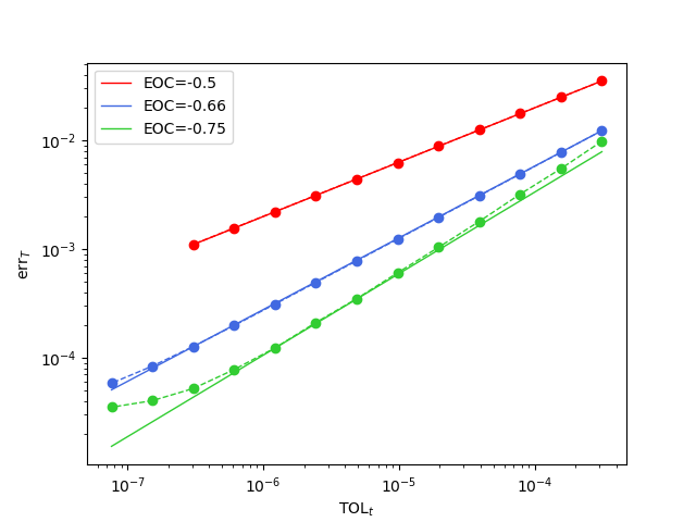
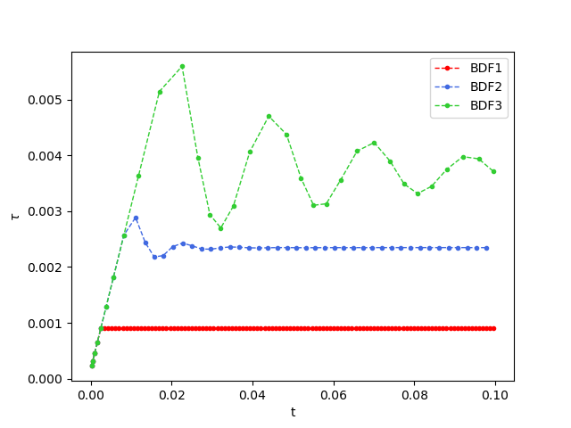
Figure 6.1. Example 6.1: Left: Convergence of $\text{err}_{T}$ for adaptive time-stepping for BDF-1 (red), BDF-2 (blue) and BDF-3 (green) with fixed $h=1/\sqrt{N_{c}}$, where $N_{c}=15488$ is the number of cells. Right: Evolution of the timestep size $\tau$ for $\mathrm{TOL}_{\mathrm{t}}=6.25\cdot 10^{-4}$.

In Figure 6.1 (left) we show the error (6.1) of the adaptive time-stepping method for BDF-1 to BDF-3 in dependence of the prescribed tolerance in time $\mathrm{TOL}_{t}$ for a fixed mesh. For BDF-$k$ we have the convergence order $k$, but local truncation error $k+1$, for uniform steps. Since we equilibrate the local truncation error we have $\tau^{k+1}\sim\mathrm{TOL}_{t}$ and therefore we observe $\text{err}_{T}\sim\mathrm{TOL}_{t}^{k/(k+1)}$. For a fixed choice of $\mathrm{TOL}_{t}$ we show in Figure 6.1 (right) the development of $\tau$ during time.

In Figure 6.2, we compare the error $\text{err}_{T}$ for uniform step sizes versus adaptive step sizes. For this purpose, we first compute the time-adaptive BDF-3 scheme for various $\mathrm{TOL}_{t}$ and store the total number of time steps $N_{t}$. Subsequently, we perform simulations with uniform step sizes, where we chose $\tau=T/N_{t}$, i. e., we need the same $N_{t}$ as in the time-adaptive simulations. We see that the adaptive algorithm leads to a smaller error for the same amount of work.

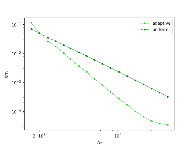
Figure 6.2. Example 6.1: Comparison of uniform step size (dark green) vs. adaptive step size (light green) computation for the BDF-3 method with fixed $h=1/\sqrt{N_{c}}$, where $N_{c}=15488$ is the number of cells.

6.2. Example 2

The following example is taken from [2, Sect. 9.2, (9.1)]. In this case we let $\Omega=(0,1)\times(0,1)$ and a source term $\boldsymbol{H}_{\mathrm{ext}}$ is provided such that the exact solution of (1.1)–(1.3) is

$$\boldsymbol{m}(t,\boldsymbol{x}) =\begin{cases}\left[\begin{smallmatrix}C_{0}(x_{1}-1/2)\,\mathrm{e}^{-\frac{g(t)}{1/4-d(\boldsymbol{x})}}\\ C_{0}(x_{2}-1/2)\,\mathrm{e}^{-\frac{g(t)}{1/4-d(\boldsymbol{x})}}\\ \sqrt{1-C_{0}^{2}d(x)\,\mathrm{e}^{-\frac{2g(t)}{1/4-d(\boldsymbol{x})}}}\end{smallmatrix}\right]\quad&\mbox{if }d(\boldsymbol{x})<1/4\,,\vspace{4pt}\\ \left[\begin{smallmatrix}0\\ 0\\ 1\end{smallmatrix}\right]&\mbox{otherwise}\,,\end{cases}$$

with $\boldsymbol{m}^{0}=\boldsymbol{m}(0)$, $g(t)=(T_{0}+0.1)/(T_{0}+0.1-t)$, $d(\boldsymbol{x})=|\boldsymbol{x}-[1,1]/2|^{2}$, $C_{0}=400$. We choose $C_{\mathrm{e}}=1$, $\alpha=0.2$, $T_{0}=0.06$ and $T=0.05$ as the final time. In this example the spatial error dominates the total error. We use $\tau=T/100$ as well as $\theta_{\mathrm{r}}=0.6$.

We perform numerical experiments for linear, quadratic and cubic finite elements on uniform and adaptive spatial meshes. Time integration is done with BDF-2. We execute Algorithm 3 with additional normalisation step for several mesh sizes $h$ and in case of space-adaption for several tolerances $\mathrm{TOL}_{s}$. In Figure 6.3 (left) we notice convergence in the error norm $\text{err}_{T}$ given by (6.1) of order one in $\mathrm{TOL}_{s}$ for all polynomial degrees until saturation occurs due to the fixed time step. However, in Figure 6.3 (right) we notice smaller errors in the error norm $\text{err}_{T}$ for higher polynomial degree if we relate these errors to the maximal degrees of freedom we obtained at a discrete time step during the simulation.

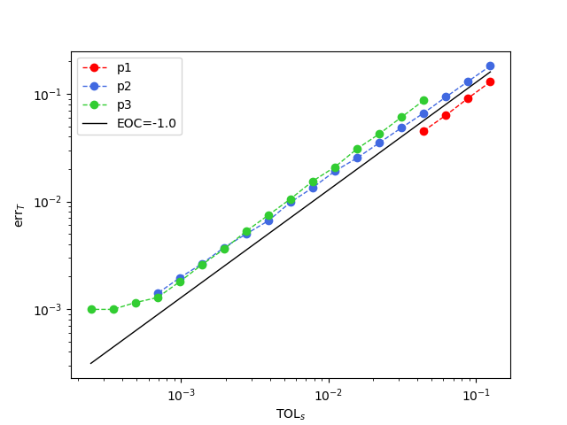
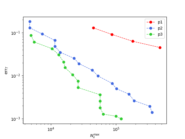
Figure 6.3. Example 6.2: Left: space tolerance $\mathrm{TOL}_{s}$ vs. $\textrm{err}_{T}$. Right: maximal degrees of freedom $N^{\text{max}}_{x}:=\max\limits_{0\leq n\leq N_{t}}\{N_{x}(t_{n})\}$ vs. $\textrm{err}_{T}$ where $N_{x}$ denotes the number of degrees of freedom and $N_{t}$ the number of time steps. Various polynomial degrees of the finite element space are presented, i.e., linear (red), quadratic (blue) and cubic (green).

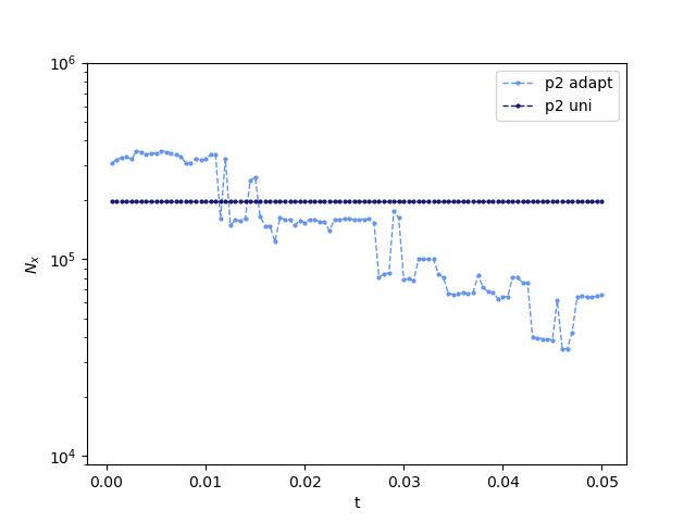
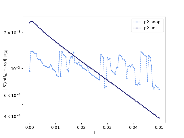
Figure 6.4. Example 6.2: Comparison between runs on uniform and adaptive spatial meshes for polynomial degree $2$. Left: Evolution of the degrees of freedom. Right: Evolution of the $H^{1}$ error. We used $\mathrm{TOL}_{s}=6.91\cdot 10^{-4}$ for the spatial tolerance.

6.3. Example 3

Here we consider an example that appears to show singular behaviour and has been considered in [10], [9], [11]. However, we will demonstrate that computations on finer meshes and particularly adaptive computations prevent a singularity from forming. We let $\Omega=(-1/2,1/2)^{2}$ and choose constants $C_{\mathrm{e}}=1$ and $\alpha=1$. We solve (1.1)–(1.3) with initial data is given by

$$\boldsymbol{m}^{0}(\boldsymbol{x}) =\begin{cases}\frac{1}{A^{2}+|\boldsymbol{x}|^{2}}\left[\begin{smallmatrix}2A\boldsymbol{x}\\ A^{2}-|\boldsymbol{x}|^{2}\end{smallmatrix}\right]\quad&\mbox{if }|\boldsymbol{x}|^{2}\leq 1/2\,,\vspace{4pt}\\ \left[\begin{smallmatrix}0\\ 0\\ -1\end{smallmatrix}\right]&\mbox{otherwise},\end{cases}$$

where $A=(1-2|\boldsymbol{x}|)^{4}/s$, $s=16$. No external field is applied, i.e., $\boldsymbol{H}_{\mathrm{ext}}=\boldsymbol{0}$. An exact solution is not known and we have to rely on qualitative behavior of the solution in order to judge the validity of the results.

We performed numerical experiments for the space- and time-adaptive Algorithm 3 and choose the mesh refinement parameter $\theta_{\mathrm{r}}=0.95$. The time integration was done with BDF-2.

In Figure 6.6 we run the algorithm for the time tolerance $\mathrm{TOL}_{t}=10^{-5}$ and space tolerance $\mathrm{TOL}_{s}=0.4$. We compare the adaptive algorithm with uniform discretizations on several meshsizes. For both, we did not apply the additional normalization step. The takaway of these experiments is that the adaptive algorithm prevents the singularity from forming with far less degrees of freedoms and thus far less computational effort than the uniform approach. This indicates that the error estimator is also useful in non-smooth situations, despite the theory only working under smoothness assumptions on the solution.

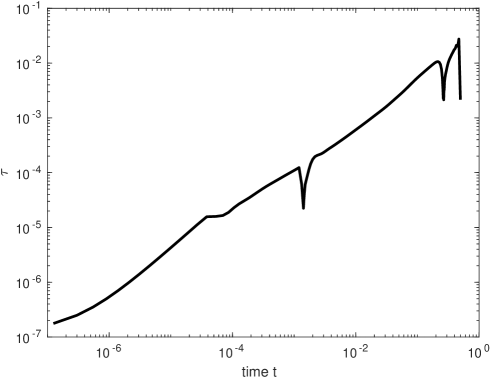
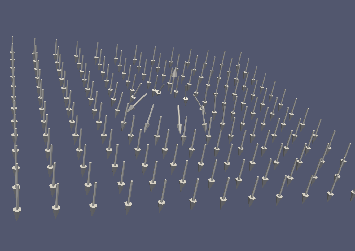
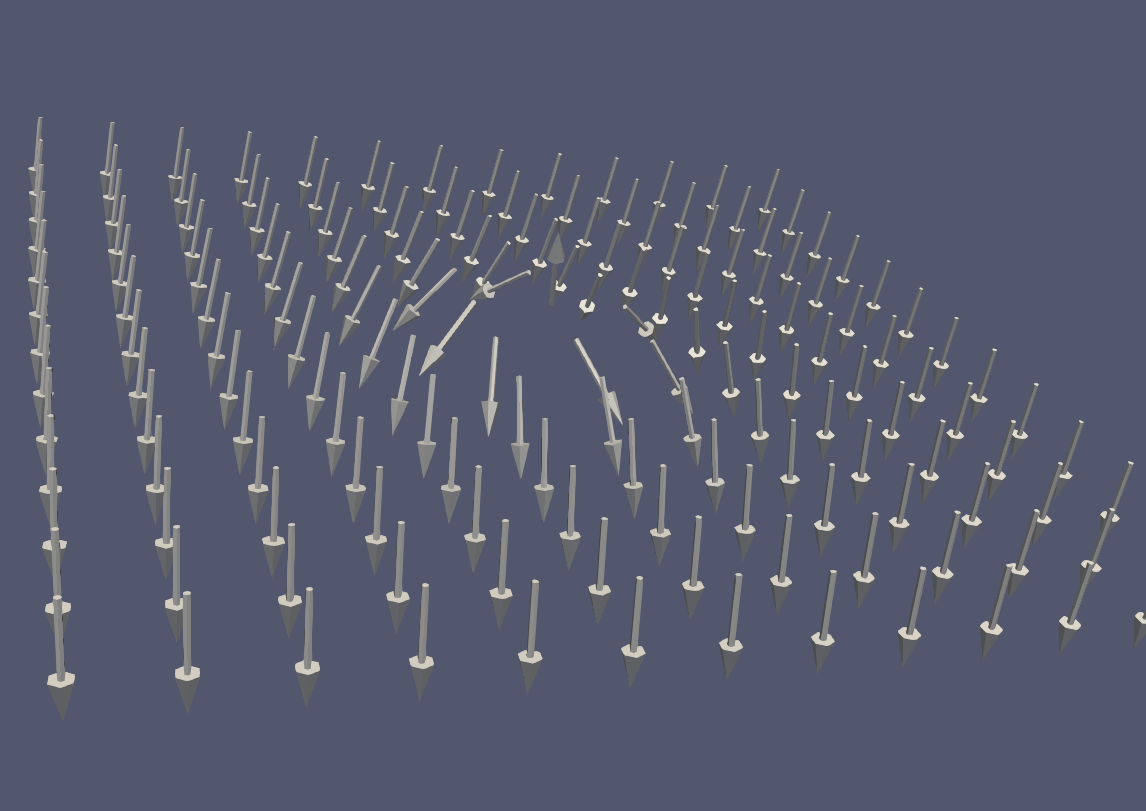
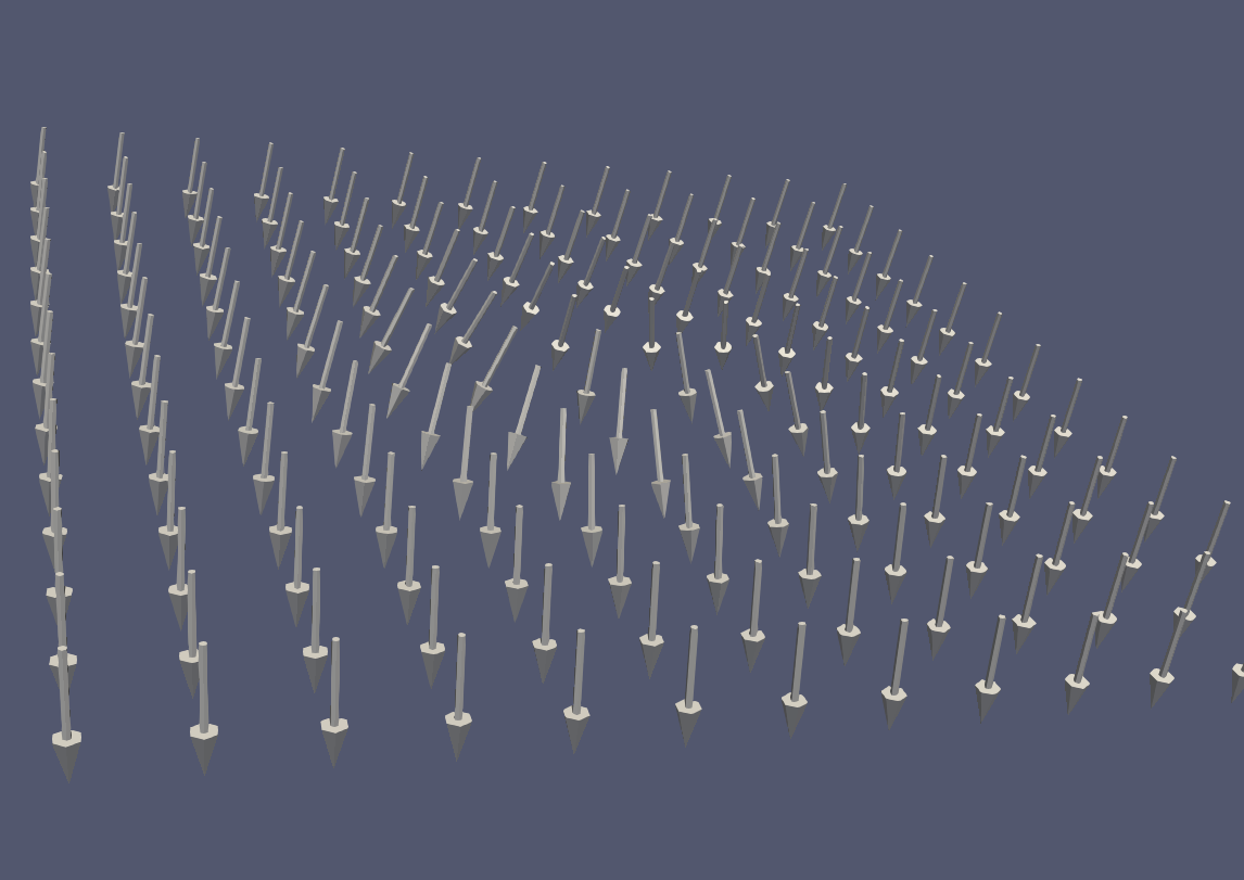
Figure 6.5. Example 6.3: Evolution of the time-step size in the adaptive computation and solution $\boldsymbol{m}_{h}$ for the uniform mesh $h=1/14$ and uniform timestep $\tau=10^{-3}$ at $t=0$ (left), $t=0.083$ (middle) and $t=0.092$ (right) according to (2.3). The singularity appears in the center of the vectorfield, where $\boldsymbol{m}$ points upward in a very small neighborhood only.

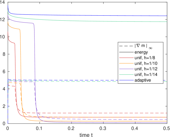
Figure 6.6. Example 6.3: We compare simulations with uniform meshes and timesteps with a fully adaptive simulation. The time step size for the uniform simulations is $\tau=10^{-3}$ and the mesh size ranges from $h=1/8$ to $h=1/14$. The adaptive simulation starts with a mesh size of $h=1/2$. The singularity, i.e., the rotation of the entire magnetization towards $[0,0,-1]$, is observed via a sharp decay of the energy. We observe that only the finest uniform simulation avoids the singularity (that requires a total number of 1261500 degrees of freedom). In contrast, the adaptive simulation achieves the same with just 209223 degrees of freedom, less than the coarsest uniform simulation.

6.4. Example 4

The following solution simulates a moving doamin wall. We take $\Omega=(0,1)\times(0,0.2)$, $T=0.35$, $C_{\mathrm{e}}=0.1$, $\alpha=1$ and provide initial data

$$\boldsymbol{m}^{0}(\boldsymbol{x}) =\begin{cases}\left[\begin{smallmatrix}0\\ 0\\ -1\end{smallmatrix}\right]&\mbox{if }x_{1}<c-d\,,\\[6.0pt] \left[\begin{smallmatrix}0\\ \cos(\pi\zeta/2)\\ \sin(\pi\zeta/2)\end{smallmatrix}\right]\quad&\mbox{if }c-d\leq x_{1}\leq c+d\,,\\[8.0pt] \left[\begin{smallmatrix}0\\ 0\\ 1\end{smallmatrix}\right]&\mbox{if }c+d\leq x_{1}\,.\end{cases}$$

for $\zeta=\sin(\pi(x_{1}-c)/2d)$, $c=0.2$, $d=0.125$. An exact solution is not known. We choose the mesh refinement parameter as $\theta_{\mathrm{r}}=0.8$. Furthermore we apply a constant external field $\boldsymbol{H}_{\mathrm{ext}}=[0,0,-50]$.

We perform numerical experiments for adaptive quadratic finite elements and adaptive time-stepping with BDF-2, where we apply the fully adaptive Algorithm 3 with additional normalisation step. We choose the tolerances $\mathrm{TOL}_{s}=10^{-4}$ and $\mathrm{TOL}_{t}=10^{-6}$.

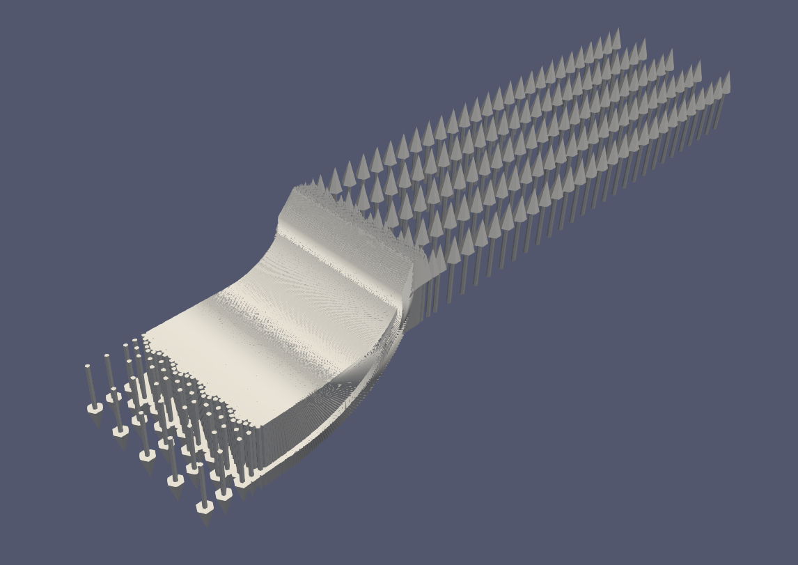
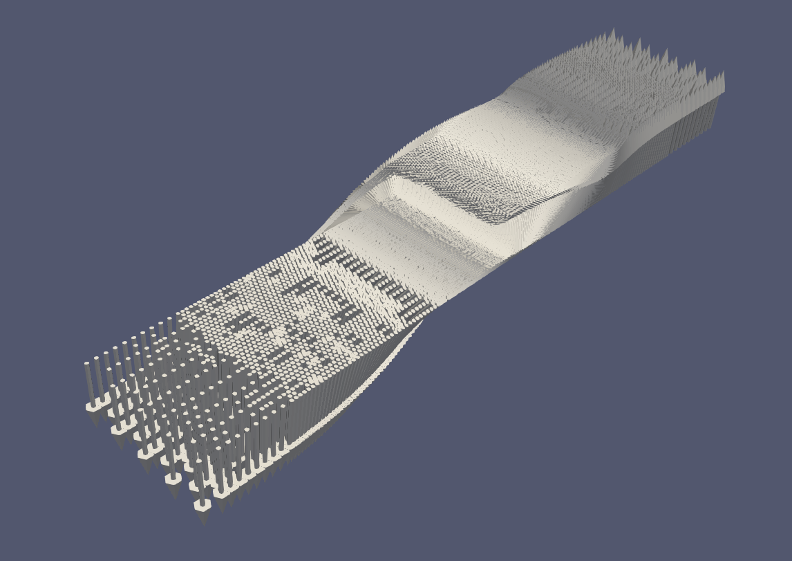
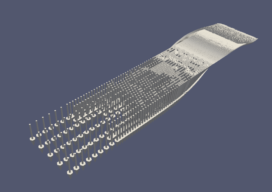
Figure 6.7. Example 6.4: Solution $\boldsymbol{m}$ at $t=0$ (left), $t=0.15$ (middle) and $t=0.3$ (right). At the final time $t=T=0.35$, all magnets are pointing downwards.

The initial configuration consists of layers of downwards and upwards pointing magnets with an intermediate layer. During the simulation the magnets pointing upwards flip their direction due to the external field and in this way the layer moves to the right (Figure 6.7). Figure 6.8 shows the obtained meshes at corresponding time instances.

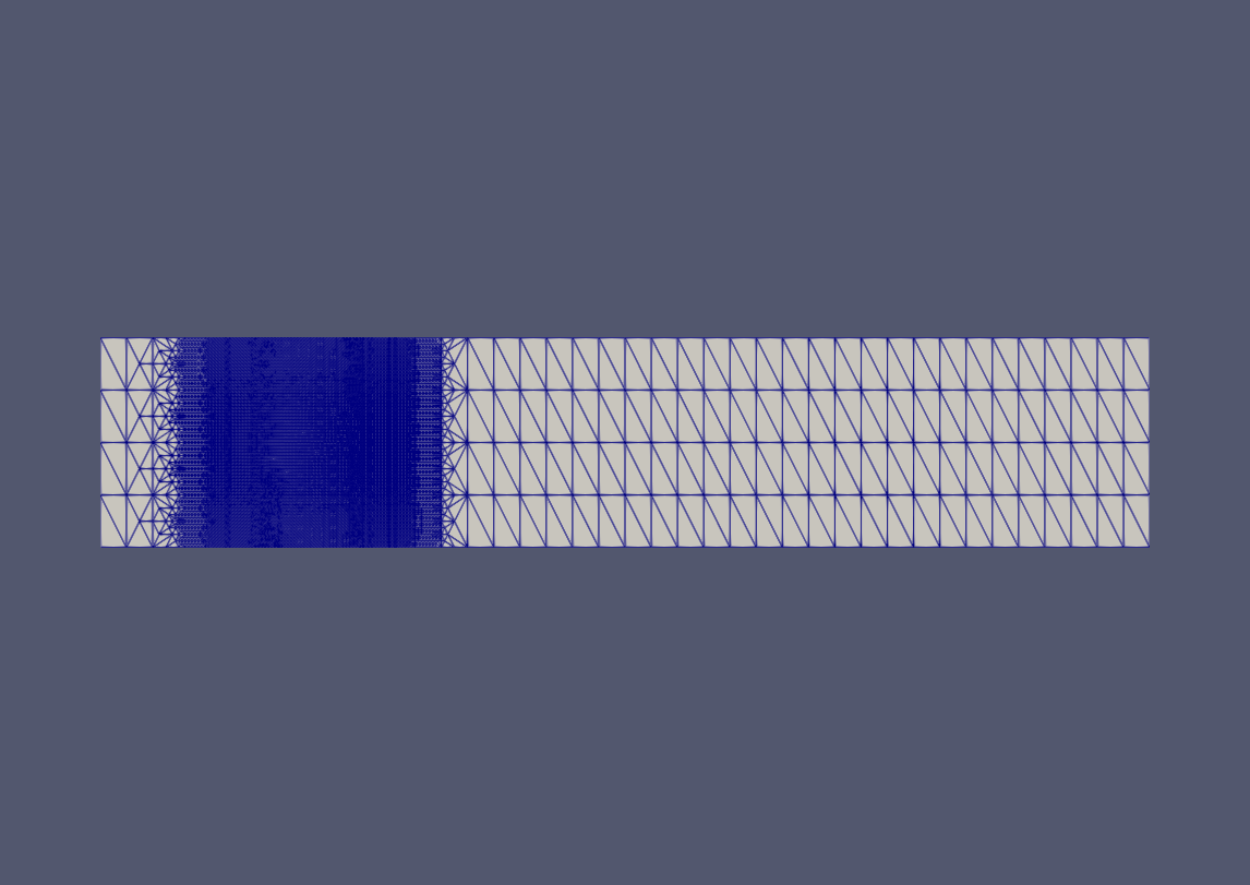
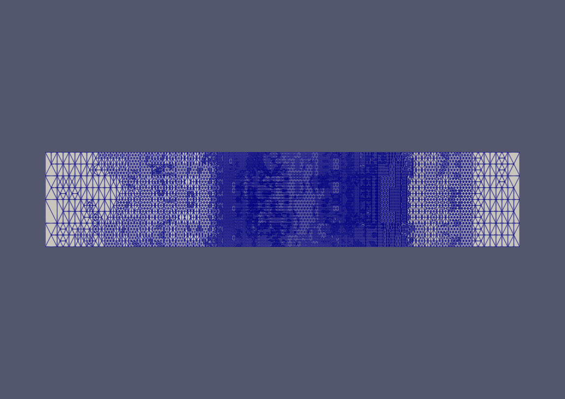
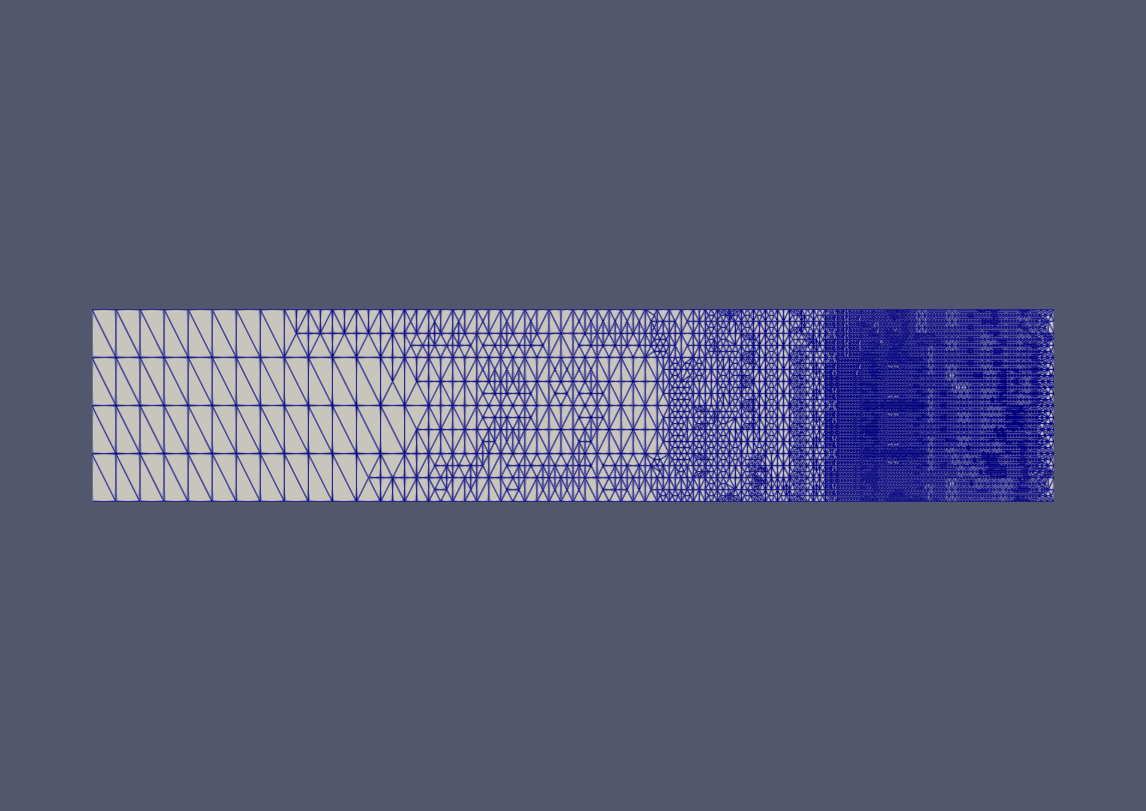
Figure 6.8. Example 6.4: Mesh at $t=0$ (left), $t=0.15$ (middle) and $t=0.3$ (right). The refined mesh moves along with the magnetic wave.

In Figure 6.9 we show the temporal development of the time step size $\tau$ (left) and the degrees of freedom $N_{x}$ (right) in case of the fully adaptive algorithm. In total, we compute $N_{t}=587$ time steps and a maximum of $440559$ degrees of freedom. After all vectors change direction, the coarsening procedure will finally lead to the initially given macro-triangulation.

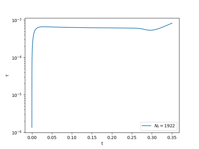
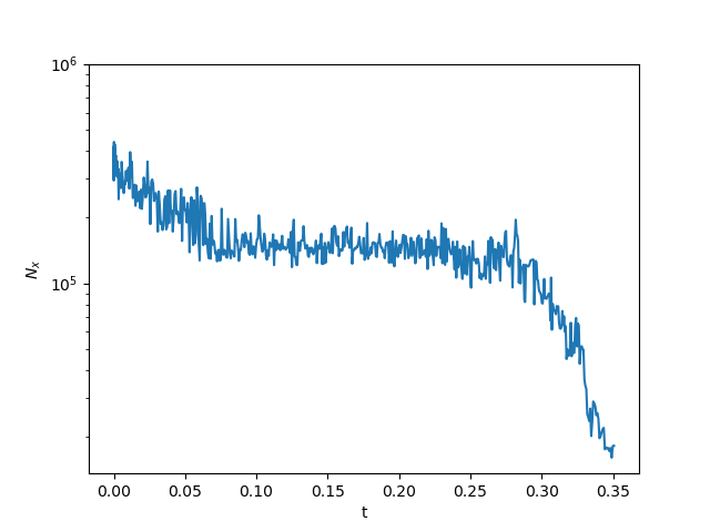
Figure 6.9. Example 6.4: Temporal development of $\tau$ (left) and the degrees of freedom $N_{x}$ (right) in case of the space- and time-adaptive algorithm.

Conclusion

We propose a time and space adaptive algorithm for the numerical approximation of the Landau–Lifshitz–Gilbert equation. Under certain regularity assumptions on the exact solutions, we show that the numerical approximation satisfies an energy inequality similar to that of the exact solution. Numerical experiments demonstrate the advantages of the adaptive algorithms over uniform approaches such as increased convergence speed (Example 6.1) or increased stability (Example 6.3). Many interesting theoretical questions still remain open for future research: Is the error estimator an upper bound for the error? Does the adaptive algorithm converge towards the exact solution? Does the energy inequality (Theorem 1) hold under reduced regularity assumptions?

Acknowledgement

Jan Bohn, Willy Dörfler, Michael Feischl and Stefan Karch gratefully acknowledge the support of the Deutsche Forschungsgemeinschaft (DFG) within the SFB 1173 “Wave Phenomena” (Project-ID 258734477).

References

- [1] Mark Ainsworth and J. Tinsley Oden. A posteriori error estimation in finite element analysis. Pure and Applied Mathematics (New York). Wiley-Interscience [John Wiley & Sons], New York, 2000.
- [2] Georgios Akrivis, Michael Feischl, Balázs Kovács, and Christian Lubich. Higher-order linearly implicit full discretization of the Landau–Lifshitz–Gilbert equation. Math. Comp., 90(329):995–1038, 2021.
- [3] Georgios Akrivis and Emmanuil Katsoprinakis. Backward difference formulae: new multipliers and stability properties for parabolic equations. Math. Comp., 85(301):2195–2216, 2016.
- [4] Martin S. Alnæs, Jan Blechta, Johan Hake, August Johansson, Benjamin Kehlet, Anders Logg, Chris Richardson, Johannes Ring, Marie E. Rognes, and Garth N. Wells. The FEniCS project version 1.5. Archive of Numerical Software, 3(100):9–23, 2015.
- [5] François Alouges. A new finite element scheme for Landau–Lifchitz equations. Discrete Contin. Dyn. Syst. Ser. S, 1(2):187–196, 2008.
- [6] Rong An. Optimal error estimates of linearized Crank–Nicolson Galerkin method for Landau–Lifshitz equation. J. Sci. Comput., 69(1):1–27, 2016.
- [7] Randolph E. Bank and Harry Yserentant. A note on interpolation, best approximation, and the saturation property. Numer. Math., 131(1):199–203, 2015.
- [8] E. Bänsch. Local mesh refinement in and dimensions. Impact Comput. Sci. Engrg., 3:181–191, 1991.
- [9] Sören Bartels, Joy Ko, and Andreas Prohl. Numerical analysis of an explicit approximation scheme for the Landau-Lifshitz-Gilbert equation. Math. Comp., 77(262):773–788, 2008.
- [10] Sören Bartels and Andreas Prohl. Convergence of an implicit finite element method for the Landau–Lifshitz–Gilbert equation. SIAM J. Numer. Anal., 44(4):1405–1419, 2006.
- [11] L’ubomír Baňas, Sören Bartels, and Andreas Prohl. A convergent implicit finite element discretization of the Maxwell–Landau–Lifshitz–Gilbert equation. SIAM J. Numer. Anal., 46(3):1399–1422, 2008.
- [12] J.-M. Coron. Nonuniqueness for the heat flow of harmonic maps. Ann. Inst. H. Poincaré C Anal. Non Linéaire, 7(4):335–344, 1990.
- [13] Giovanni Di Fratta, Michael Innerberger, and Dirk Praetorius. Weak-strong uniqueness for the Landau-Lifshitz-Gilbert equation in micromagnetics. Nonlinear Anal. Real World Appl., 55:103122, 13, 2020.
- [14] Giovanni Di Fratta, Carl-Martin Pfeiler, Dirk Praetorius, Michele Ruggeri, and Bernhard Stiftner. Linear second-order IMEX-type integrator for the (eddy current) Landau-Lifshitz-Gilbert equation. IMA J. Numer. Anal., 40(4):2802–2838, 2020.
- [15] Michael Feischl and Thanh Tran. The eddy current–LLG equations: FEM-BEM coupling and a priori error estimates. SIAM J. Numer. Anal., 55(4):1786–1819, 2017.
- [16] Michael Feischl and Thanh Tran. Existence of regular solutions of the Landau–Lifshitz–Gilbert equation in 3D with natural boundary conditions. SIAM J. Math. Anal., 49(6):4470–4490, 2017.
- [17] Riccardo Ferrero and Alessandra Manzin. Adaptive geometric integration applied to a 3d micromagnetic solver. Journal of Magnetism and Magnetic Materials, 518:167409, 2021.
- [18] Albert Fert, Vincent Cros, and Joao Sampaio. Skyrmions on the track. Nat. Nanotechnol., 8:152–156, 2013.
- [19] Huadong Gao. Optimal error estimates of a linearized backward Euler FEM for the Landau–Lifshitz equation. SIAM J. Numer. Anal., 52(5):2574–2593, 2014.
- [20] T. Gilbert. A Lagrangian formulation of the gyromagnetic equation of the magnetic field. Phys Rev, 100:1243–1255, 1955.
- [21] Rolf Dieter Grigorieff. Stability of multistep-methods on variable grids. Numer. Math., 42(3):359–377, 1983.
- [22] E. Hairer and G. Wanner. Solving ordinary differential equations. II, volume 14 of Springer Series in Computational Mathematics. Springer-Verlag, Berlin, 2010. Stiff and differential-algebraic problems, Second revised edition, paperback.
- [23] Gino Hrkac, Carl-Martin Pfeiler, Dirk Praetorius, Michele Ruggeri, Antonio Segatti, and Bernhard Stiftner. Convergent tangent plane integrators for the simulation of chiral magnetic skyrmion dynamics. Adv. Comput. Math., 45(3):1329–1368, 2019.
- [24] E. Kritsikis, A. Vaysset, L. D. Buda-Prejbeanu, F. Alouges, and J.-C. Toussaint. Beyond first-order finite element schemes in micromagnetics. J. Comput. Phys., 256:357–366, 2014.
- [25] L. Landau and E. Lifshitz. On the theory of the dispersion of magnetic permeability in ferromagnetic bodies. Phys. Z. Sowjetunion, 8:153–168, 1935.
- [26] Dirk Praetorius, Michele Ruggeri, and Bernhard Stiftner. Convergence of an implicit-explicit midpoint scheme for computational micromagnetics. Comput. Math. Appl., 75(5):1719–1738, 2018.
- [27] Andreas Prohl. Computational micromagnetism. Advances in Numerical Mathematics. B. G. Teubner, Stuttgart, 2001.
- [28] Thomas Schrefl. Finite elements in numerical micromagnetics. Part I: Granular hard magnets. Journal of Magnetism and Magnetic Materials, 207(1):45–65, 1999.
- [29] D. Weller et al. FePt heat assisted magnetic recording media. Journal of Vacuum Science & Technology B, Nanotechnology and Microelectronics, 34, 2016.