Kinematics, Structure, and Mass Outflow Rates of Extreme Starburst Galactic Outflows
Abstract
We present results on the properties of extreme gas outflows in massive (10), compact, starburst () galaxies at z = with very high star formation surface densities (). Using optical Keck/HIRES spectroscopy of 14 HizEA starburst galaxies we identify outflows with maximum velocities of . High-resolution spectroscopy allows us to measure precise column densities and covering fractions as a function of outflow velocity and characterize the kinematics and structure of the cool gas outflow phase (T 104 K). We find substantial variation in the absorption profiles, which likely reflects the complex morphology of inhomogeneously-distributed, clumpy gas and the intricacy of the turbulent mixing layers between the cold and hot outflow phases. There is not a straightforward correlation between the bursts in the galaxies’ star formation histories and their wind absorption line profiles, as might naively be expected for starburst-driven winds. The lack of strong Mg II absorption at the systemic velocity is likely an orientation effect, where the observations are down the axis of a blowout. We infer high mass outflow rates of 50 2200 , assuming a fiducial outflow size of 5 kpc, and mass loading factors of 5 for most of the sample. While these values have high uncertainties, they suggest that starburst galaxies are capable of ejecting very large amounts of cool gas that will substantially impact their future evolution.
1 Introduction
In the last decade, the potential impact of galaxy-scale outflows in galactic evolution has become widely recognized (e.g., Kormendy & Ho, 2013; Somerville & Davé, 2015; Veilleux et al., 2020). Outflows provide a mechanism that can regulate and possibly quench star formation activity in the galaxy by blowing away the gas that feeds star formation and supermassive black hole (SMBH) growth, enriching the large-scale galactic environment with metals. Theoretical studies and simulations show that this “feedback” offers a natural explanation for a variety of observations, e.g., the chemical enrichment of the circumgalactic and intergalactic medium (CGM, IGM), the self-regulation of the growth of the SMBH and of the galactic bulge, the relative dearth of both low and high mass galaxies in the stellar mass function, and the existence of the red sequence of massive, passive galaxies (e.g., Silk & Rees, 1998; Thompson et al., 2005; Kereš et al., 2005; Oppenheimer et al., 2010; Murray et al., 2010; Tumlinson et al., 2017; Davies et al., 2019; Nelson et al., 2019). While galactic outflows appear to be crucial to rapidly shutting down star formation, the physical drivers of this ejective feedback are still unclear. In particular, the relative role of feedback from stars versus SMBHs in quenching star formation in massive galaxies remains widely debated.
Our team has been studying a sample of massive (M1011 M⊙) galaxies at z = 0.40.8, originally selected from the Sloan Digital Sky Survey (SDSS; York et al., 2000) Data Release 8 (DR8; Aihara et al., 2011) to have typical signatures of young post-starburst galaxies. We refer to these galaxies as the HizEA111HizEA was originally coined as shorthand for High- E+A, meaning high redshift post-starburst. However, subsequent work has shown that many of the galaxies host on-going starbursts (see Section 2.2). sample. Their spectra exhibit both strong stellar Balmer absorption from A- and B-stars and weak or absent nebular emission lines, implying minimal ongoing star formation. These galaxies are driving extremely fast ionized gas outflows, as revealed by highly blueshifted Mg II absorption in 90% (Davis et al., submitted) of their optical spectra, with velocities of 10002500 , an order of magnitude larger than typical z 1 star-forming galaxies (e.g., Weiner et al., 2009; Martin et al., 2012). These results initially led our team to conclude that these galaxies are post-starburst systems with powerful outflows that may have played a critical role in quenching their star formation (Tremonti et al., 2007).
However, several of these galaxies are detected in the Wide-field Infrared Survey Explorer (WISE; Wright et al., 2010), and their ultraviolet (UV) to near-IR spectral energy distributions (SEDs) indicate a high level of heavily obscured star formation ( 50 M⊙ yr-1; Diamond-Stanic et al., 2012). Furthermore, Hubble Space Telescope (HST) imaging of 29 of these galaxies reveals they are in the late stages of highly dissipational mergers with exceptionally compact central starforming regions (few 100 pc; Diamond-Stanic et al., 2012, 2021; Sell et al., 2014). Combining star formation rate (SFR) estimates from WISE rest-frame mid-IR luminosities with physical size estimates from HST imaging, we derive extraordinarily high SFR surface densities 103 M⊙ yr-1 kpc-2 (Diamond-Stanic et al., 2012), approaching the maximum allowed by stellar radiation pressure feedback models (Lehnert & Heckman, 1996; Meurer et al., 1997; Murray et al., 2005; Thompson et al., 2005). These findings paint a different picture where our targets are starburst galaxies with dense, dusty star-forming cores (Perrotta et al., 2021), and a substantial portion of their gas and dust is blown away by powerful outflows. Millimeter observations for two galaxies in our sample suggest that the reservoir of molecular gas is being consumed by the starburst with remarkable efficiency (Geach et al., 2013), and ejected in a spatially extended molecular outflow (Geach et al., 2014), leading to rapid gas depletion times. Notably, we find little evidence of ongoing AGN activity in these systems based on X-ray, IR, radio, and spectral line diagnostics (Sell et al., 2014; Perrotta et al., 2021). These results agree with models in which stellar feedback is the primary driver of the observed outflows (e.g. Hopkins et al., 2012, 2014). Our sample of compact starburst galaxies is characterized by the highest and the fastest outflows (1000 ) observed among star-forming galaxies at any redshift; therefore, they are an ideal laboratory to test the limits of stellar feedback and determine whether stellar processes alone can drive extreme outflows, without the need to invoke feedback from SMBH. They could represent a short but relatively common phase of massive galaxy evolution (Whalen et al., 2022).
Low and medium-resolution observations have shown that large-scale galactic outflows are a common feature of star-forming galaxies across a wide range of masses and redshifts (e.g., Martin, 1998; Heckman et al., 2000; Weiner et al., 2009; Martin & Bouché, 2009; Martin et al., 2012; Rubin et al., 2010, 2014; Heckman et al., 2015; Heckman & Borthakur, 2016; McQuinn et al., 2019). Thanks to these studies we have a fair understanding of the typical outflow kinematics, and how their main properties scale with the fundamental properties of their galaxy hosts. While absorption-line spectroscopy at low and medium resolution is sufficient to measure velocities and the total amount of absorption within outflows, robust determinations of key physical properties such as the column density, covering fraction, and mass outflow rate require high spectral resolution. In this paper, we present new optical Keck/HIRES observations for 14 of the most well-studied starburst galaxies in our sample. These high-resolution spectra allow us to directly measure accurate column densities and covering fractions as a function of velocity for a suite of Mg and Fe absorption lines. We utilize this to probe the small scale structures of the extreme galactic outflows observed in our sample and investigate the potential impact of these outflows on the evolution of their host galaxies.
The paper is organized as follows: Section 2 describes the sample selection, observations, and data reduction; Section 3 illustrates our line profile fitting method and measurements of the absorption line column densities and kinematics; Section 4 presents our main results in comparison to theoretical models and other galaxy samples, and discusses the more comprehensive implications of our analysis. Our conclusions are reviewed in Section 5.
2 Sample and Data Reduction
The parent sample for this analysis was selected from the Sloan Digital Sky Survey I (SDSS-I York et al., 2000) Data Release 8 (DR8; Aihara et al., 2011) and is described in Tremonti et al. (2007); Diamond-Stanic et al. (2012); Sell et al. (2014); Diamond-Stanic et al. (2021) and Davis et al., (submitted). Briefly, as mentioned above, the original goal was to identify a sample of intermediate redshift (z = ) post-starburst galaxies to investigate their star formation quenching mechanisms. We focused on redshift 0.35 so that the Mg II2796, 2803 doublet, an ISM line broadly used to probe galactic winds, was easily observable with optical spectrographs. Since the SDSS main galaxy sample (Strauss et al., 2002) is magnitude limited (r 17.7) and does not contain many galaxies at z 0.25, we concentrated on objects targeted for spectroscopy as quasars because they probe fainter magnitudes (i 20.4) and higher redshifts. We selected all objects classified by the SDSS spectroscopic pipeline as galaxies with redshifts between z = and either g 20 or i 19 mag (296 galaxies). To select galaxies with a recent ( 1 Gyr) burst of star formation, but little ongoing activity, we required them to show strong Balmer-absorption (suggestive of a burst Myr ago) and moderately weak nebular emission (suggestive of a low SFR in the past 10 Myr). Removing 3% of the objects by visual examination (blazars or odd quasars with wrong redshifts) yielded a sample of 121 galaxies. More details about the sample selection can be found in Tremonti et al., (in prep.) and Davis et al., (submitted).
We have undertaken extensive follow-up observations on a subsample of 50 of these galaxies. In choosing this subsample, we prioritized galaxies with the largest g-band fluxes and the youngest stellar populations, but we included galaxies with older burst ages for comparison. The sample comprises galaxies with mean stellar ages in the range of 4 - 400 Myr. Notably, we did not prioritize galaxies with Mg II absorption lines.
We obtained ground-based spectroscopy of the 50/121 galaxies with the MMT/Blue Channel, Magellan/MagE, Keck/LRIS, Keck/HIRES, and/or Keck/KCWI (Tremonti et al., 2007; Diamond-Stanic et al., 2012; Sell et al., 2014; Rupke et al., 2019), X-ray imaging with Chandra for 12/50 targets (Sell et al., 2014), radio continuum data with the NSF’s Karl G. Jansky Very Large Array (JVLA/VLA) for 20/50 objects (Petter et al., 2020), millimeter data (ALMA) for 2/50 targets (Geach et al., 2014, 2018), and optical imaging with HST for 29/50 galaxies (“HST sample” Diamond-Stanic et al., 2012; Sell et al., 2014; Diamond-Stanic et al., 2021). For the HST observations, we first targeted the twelve galaxies that were most likely to have AGN. We observed three galaxies with broad Mg II emission (expected to be type I AGN) and nine galaxies with strong [O III] emission, which could be indicative of an obscured (type II) AGN. We subsequently observed an additional seventeen galaxies that have the youngest estimated post-burst ages (tburst 300 Myr). We also obtained multi-band HST imaging to study the physical conditions at the centers of the 12/29 galaxies with the largest SFR surface densities estimated by Diamond-Stanic et al. (2012), (30 M yr-1 kpc-2 2000 M yr-1 kpc-2), and investigated the young compact starburst component that makes them so extreme (Diamond-Stanic et al., 2021).
In this paper, we focus on 14 galaxies from the HST sample (6 from the 12/29 most AGN-like galaxies, and 8 from the 17/29 with the youngest post-burst ages). The galaxies and their basic properties are listed in Table 1.
2.1 Data Acquisition and Reduction
We obtained high–resolution spectra of 14 starburst galaxies spanning emission redshifts 0.4 z 0.8, using the Keck High Resolution Echelle Spectrometer (HIRES; Vogt et al., 1994) on the Keck I telescope over the nights of August 2009, December 2009, and May 2012. HIRES was configured using the 1.148 7 arcsec C5 decker with no filters and 2x2 binning. The 1.148 arcsec slit width disperses the light with R = / = 37,000 ( 8 ) projected to 3 pixels per resolution element, . Individual exposures were 3600 seconds, with total integration times of hours per object.
This yielded an observed wavelength coverage from 3150 to 5800 Å in 30 orders, which for our galaxies corresponds to a rest-frame coverage from 18003250 to Å depending on redshift. We concentrate our analysis on the Mg II2796, 2803 doublet, the Mg I2852 transition, and the Fe II2344, 2374, 2582, 2587, and 2600 multiplet.
| ID | zsys | RA | Dec | log(M∗/M⊙) | re | SFR | LW Age | |
|---|---|---|---|---|---|---|---|---|
| J2000 | J2000 | kpc | M⊙ yr-1 | M⊙ yr-1 kpc-2 | Myr | |||
| (1) | (2) | (3) | (4) | (5) | (6) | (7) | (8) | (9) |
| J0826+4305 | 0.603 | 126.66006 | 43.091498 | 10.63 | 0.173 | 184 | 981 | 22 |
| J0901+0314 | 0.459 | 135.38926 | 3.236799 | 10.66 | 0.237 | 99 | 281 | 54 |
| J0905+5759 | 0.711 | 136.34832 | 57.986791 | 10.69 | 0.097 | 90 | 1519 | 17 |
| J0944+0930 | 0.514 | 146.07437 | 9.505385 | 10.59 | 0.114 | 88 | 1074 | 88 |
| J11250145 | 0.519 | 171.32874 | -1.759006 | 11.03 | 0.600 | 227 | 100 | 102 |
| J1219+0336 | 0.451 | 184.98241 | 3.604417 | 10.35 | 0.412 | 91 | 85 | 22 |
| J1232+0723 | 0.400 | 188.06593 | 7.389085 | 10.93 | 2.200 | 62 | 2 | 79 |
| J13410321 | 0.661 | 205.40333 | -3.357019 | 10.53 | 0.117 | 151 | 1755 | 14 |
| J1450+4621 | 0.782 | 222.62024 | 46.360473 | 11.06 | 0.540 | 191 | 104 | 107 |
| J1506+5402 | 0.608 | 226.65124 | 54.039095 | 10.60 | 0.168 | 116 | 652 | 13 |
| J1558+3957 | 0.402 | 239.54683 | 39.955787 | 10.42 | 0.778 | 84 | 22 | 44 |
| J1613+2834 | 0.449 | 243.38552 | 28.570772 | 11.12 | 0.949 | 172 | 30 | 72 |
| J21160624 | 0.728 | 319.10479 | -6.579113 | 10.41 | 0.284 | 110 | 216 | 21 |
| J2140+1209∗ | 0.752 | 325.00205 | 12.154051 | 10.36 | 0.153 | 24 | 163 | 192 |
Note. — Column 2: Galaxy systemic redshift. Column 5: Stellar mass from Prospector. Column 6: Effective radii from HST. Column 7: SFRs from Prospector. Column 8: SFR surface densities estimated using columns (6) and (7). Column 9: Light-weighted ages of the stellar populations younger than 1 Gyr.
The data were reduced using the XIDL HIRES Redux code222Available at https://www.ucolick.org/~xavier/HIRedux/index.html. We used this reduction pipeline to perform flat-field corrections, determine wavelength solutions using thorium-argon (ThAr) arcs, measure slit profiles for each order, perform sky subtraction, and remove cosmic rays. The output of the spectral extraction is an order-by-order spectrum of counts versus vacuum wavelength. For a more comprehensive description of this procedure, we refer the reader to O’Meara et al. (2015). As automated flux calibration of HIRES spectra is unreliable (e.g., Suzuki et al., 2005), each echelle order was examined by eye to perform continuum fitting. A Legendre polynomial was fit to each order and adjusted using anchor points in absorption-free regions with a custom IDL code.
2.2 Galaxy properties
We report in Table 1 relevant derived galaxy properties for our sample. Accurate systemic redshifts are necessary in order to determine outflow velocities. For this purpose, we use stellar continuum fits as derived in Davis et al. (submitted). We have collected low/medium resolution (R = ) optical spectra of our parent sample (50 galaxies) using three instruments on -m class telescopes (MMT/Blue Channel, Magellan/MaGE, and Keck/LRIS; see Davis et al. (submitted) and Tremonti et al. in prep. for details on these data sets). We required our spectra to extend to at least 4000 Å in the restframe to cover strong stellar or nebular features to aid in measuring the galaxy systemic redshift (e.g. [O II], low order Balmer absorption lines). We fit the spectra with a combination of SSP models and a Salim et al. (2018) reddening law derived from local galaxies that are analogs of massive, high redshift galaxies. We used the Flexible Stellar Population Synthesis code (Conroy et al., 2009; Conroy & Gunn, 2010) to generate SSPs with Padova 2008 isochrones (Marigo et al., 2008), a Salpeter (1955) initial mass function (IMF), and the theoretical stellar library C3K (Conroy et al., in prep.) with a resolution of R 10,000. We utilize solar metallicity SSP templates with 43 ages spanning 1 Myr 8.9 Gyr and perform the fit with the Penalized Pixel-Fitting (pPXF) software (Cappellari & Emsellem, 2004; Cappellari, 2017). We mask the region around Mg II and the forbidden emission lines during the fit and implement two separate templates for broad and narrow Balmer emission lines, assuming Case B recombination line ratios. Both the lines and stellar continuum are attenuated by the same amount of dust in the pPXF fit; we find that the results are insensitive to this assumption. By fitting Balmer emission and absorption lines simultaneously we can take into account the potential infill of the absorption line cores. One of the outputs of our pPXF fit is the galaxy systemic redshift (zsys), which we list in Table 1.
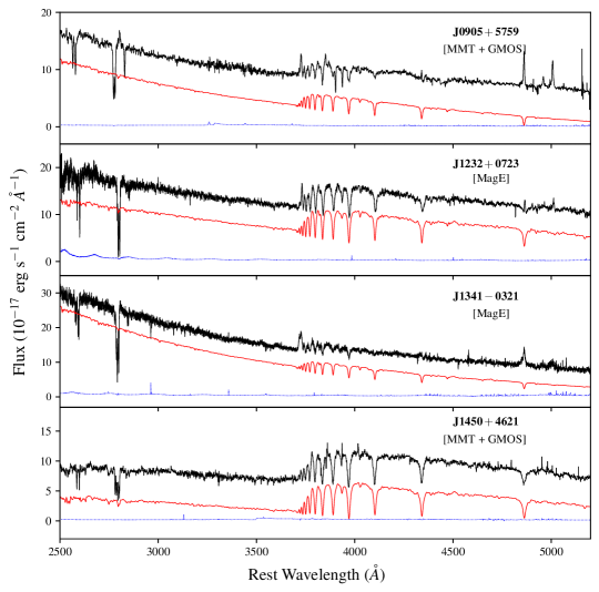
The fit produces a stellar continuum model without a nebular emission component (see Figure 1). Most sources, in addition to having strong Balmer absorption, have very blue continua indicating a recent starburst event (110 Myr) that is not highly dust-obscured. For galaxies with young stellar populations, like those in our sample, the stellar contribution to the Mg absorption lines is minimal. However, we utilize our best fit pPXF continuum model to properly remove the stellar absorption features from each spectrum in our sample.
To estimate stellar masses (M∗) and star formation rates (SFR) we fit the combined broad-band UV – mid-IR photometry and optical spectra using the Bayesian SED code Prospector (Leja et al., 2019; Johnson et al., 2021), as described in Davis et al. (submitted). Briefly, we incorporate the 3500 - 4200 Å spectral region in the SED fit as it covers many age-sensitive features (e.g., D4000, H). We generate simple stellar population (SSP) models employing the Flexible Stellar Populations Synthesis code (FSPS; Conroy et al., 2009), adopting a Kroupa IMF (Kroupa, 2001) and the MIST isochrones (Choi et al., 2016) and the C3K stellar theoretical libraries (Conroy et al., in prep.). The stellar models are very similar to the ones described above over the wavelength range of interest for this work. We determined the best-fit parameters and their errors from the 16th, 50th, and 84th percentiles of the marginalized probability distribution function. The combined photometry and spectra are well fit by these models (see Davis et al., submitted for examples of the SED fitting). However, the dust emission properties of our sample are poorly constrained due to the low signal-to-noise ratio (SNR) of the WISE W3 and W4 photometry and the limited infrared coverage of the SED. This yields fairly tight constraints on the M∗ (0.15 dex) and slightly larger errors on the SFR (0.2 dex). M∗ represents the present-day stellar mass of the galaxy (after accounting for stellar evolution) and not the integral of the star formation history (i.e. total mass formed). We list in Table 1 the SFRs calculated from the resulting star formation history (SFHs; see Fig. 9), averaged over the last 100 Myr. This is the typical timescale for which UV and IR star formation indicators are sensitive (Kennicutt & Evans, 2012). As here we are interested in the most recent SFH, we compute the light-weighted age of the stellar populations younger than 1 Gyr, with the light contribution estimated at 5500 Å. These 1 Gyr light-weighted ages more closely replicate the timescale of the peak SFR than the mass-weighted ages. We use light-weighted ages rather than the age since the burst as the light-weighted ages are more robust to changes in our modeling approach. However, there may be systematic errors related to the stellar population models we adopt. In practice uncertainties in the treatment of Wolf-Rayet stars and high mass binary evolution can have a large impact on the UV spectra of galaxies with young stellar populations (e.g. Eldridge & Stanway, 2016). The detailed analysis required to produce a quantitative estimate of the systematic errors on the light-weighted ages is beyond the scope of this work. The light-weighted ages for the galaxies in our sample are reported in Table 1.
The effective radii (re) measurements for the galaxies in our sample are discussed in Diamond-Stanic et al. (2012, 2021). Briefly, for 11 galaxies we use the GALFITM software (Häußler et al., 2013; Vika et al., 2013) to perform Sérsic fits of joint multi-band HST imaging (Diamond-Stanic et al., 2021) in the UVIS/F475W and UVIS/814W filters. To prevent uncertainties due to tidal features, we fit the central region of the galaxy and extrapolate the fit to larger radii to compute re. The shorter-wavelength filter ((F475W) 3000Å) traces the young, unobscured stars, while the longer-wavelength filter ((F814W) 5200Å) is more sensitive to the underlying stellar mass. Characteristic errors on the effective radius are of the order of 20%. For the remaining three galaxies (J1125, J1232, and J1450) we quantify the morphology utilizing optical HST UVIS/F814W image (Diamond-Stanic et al., 2012). We model the two-dimensional surface brightness profile with a single Sersic component (defined by Sersic index = 4 and re) using GALFIT (Peng et al., 2002, 2010). We adopt an empirical model point-spread function (PSF) produced using moderately bright stars in our science images.
3 Spectral Analysis
In this section, we briefly present our data, discuss the method and assumptions adopted for the line profile fitting and describe the techniques used to estimate errors. The line fitting results for each galaxy are listed in Tables 2 and 3.
3.1 Absorption Lines as Tracers of Galactic Outflows
Galactic winds are typically recognized through their kinematic signatures. Winds seen in absorption are identified as troughs detected in the foreground of the galaxy stellar continuum, blueshifted with respect to the galaxy systemic velocity (e.g., Martin & Bouché, 2009; Martin et al., 2012; Kornei et al., 2012; Rubin et al., 2014; Prusinski et al., 2021). In this context the line velocity shift relative to the systemic redshift () at which 98% () or 50% (vavg) of the equivalent width (EW) accumulates moving from red (positive velocities) to blue (negative velocities) across the line profile can be used to parameterize the kinematics of absorption lines.
The galaxies in our sample commonly display extreme kinematics in the Mg II absorption lines. Figure 2 shows the continuum-normalized Mg II spectral region for each galaxy and illustrates the range of spectral absorption properties in our data. The Mg II2796, 2803 absorption lines are produced by the blending of multiple velocity components. Additionally, the Mg II2796 line has blueshifted components that blend with the Mg II2803 components in almost all of the galaxies (with the exception of J1125 and J2116). The velocity blueshifts that cause this blending range from several hundred up to over 2,000 in the Mg II absorbing gas. Given the complex kinematics, we cannot directly integrate the spectrum to measure the EW of the single absorption components. However, we can calculate the total Mg II EW by integrating the normalized spectrum over the velocity range for which we detect Mg II absorption. The total rest frame EWs for the galaxies in our sample are reported at the bottom of each panel in Figure 2. The Mg II absorption lines are very strong, with EWs from 1.89 to 12.90 Å, with an average value of 7.49 Å. (Below in Section 4.4 we compare our galaxies to other samples in the literature.) The values in the Mg II absorption lines span a range from to , with an average value of . Such large line blueshifts are unambiguous signs of outflowing gas. We note that the potential emission filling effects on the estimates are negligible (see Section 4.2). In the following section, we construct a model that describes our data in order to quantify the kinematics and strength of the outflows.
3.2 Line Fitting
We refer the reader to Rupke et al. (2005a) for a complete discussion of the analysis techniques used in absorption line fitting, depending on the type of line profiles studied. Here we summarize the relevant aspects for our sources which have partially covered, blended absorption lines.
The profile of a single absorption trough is parameterized by the distribution of the optical depth () along the line of sight, combined with how the absorbing gas covers the background source. If it completely covers the background source, such that the covering fraction () is unity, then the distribution can be calculated accurately as a function of velocity. This is valid also for a blended doublet, triplet, or higher-order multiplet lines which can be fit by solving a set of linear equations, using a “regularization” method (Arav et al., 1999). However, when the background light source subtends a wide angle on the sky compared to the absorbing clouds, is generally less than unity. This latter case may apply to our sample, where the central starburst illuminates gas clouds in the galaxy halo.
The intensity of an absorption line, where and depend on velocity and the continuum level has been normalized to unity, can be described as . There is a degeneracy when solving for and for a single line. This degeneracy can usually be resolved by simultaneously fitting two or more transitions of the same species with known oscillator strengths (), as the relative depths of the lines are independent of . However, in the case of doublet or higher-order multiplet lines blended together, we cannot solve for and directly, as in the region of overlap the solution is not unique. Nor can we directly integrate the spectrum to estimate the EW of the single absorption troughs. We must thus fit analytic functions to the line profiles. We, therefore, use intensity profiles which are direct functions of physical parameters (i.e., velocity, optical depth, and covering fraction). We assume can be formulated as a Gaussian, , where and are the central wavelength and central optical depth of the line, and is the velocity width of the line (or Doppler parameter ). The clear advantage of this approach is that the derived profile shapes are readily interpreted in terms of these physical parameters. This method accurately handles the intensity profile at both low and high optical depth in the case of constant which is an assumption we make for simplicity.
To decompose the blended absorption profiles, we need to make assumptions about the geometry of the absorbing gas. Here we refer to “components” to describe distinct velocity components of the same transition.
We assume the case of completely overlapping atoms when combining the intensities of two doublet or multiplet lines within a given velocity component. In this context, the atoms at all velocities are placed at the same position in the plane of the sky relative to the background continuum source. This is a simplification, as the broad profiles we observe could be due to the large-scale motions of individual clouds that are not all coincident. The covering fraction in this case is independent of velocity. The expression for the combined intensity of a doublet or multiplet (each with optical depth and covering fraction )) is then given by
| (1) |
We assume the case of partially overlapping atoms when combining two different velocity components. The motivation for this is that different components could have different if we assume they are spatially distinct. In this scenario, at a given wavelength there is an overlap between the atoms producing the components, and the covering fraction describes the fractional coverage of both the continuum source and the atoms producing the other component. The definition of the intensity is
| (2) |
We fit our data utilizing a suite of IDL routines from the IFSFIT library (Rupke, 2014). The code combines the two cases illustrated above when simultaneously fitting doublet lines that have multiple blended velocity components. We describe the normalized line profile intensity for each component as a function of four parameters: , , , and column density (). can be formulated as
| (3) |
Different transitions of the same ionic species are required to have the same component structure and are fit simultaneously to produce a single solution. However, we do not impose the same kinematics on different ionization states of the same element or on other elements. As we impose no constraints on the decomposition between different ionization states or different ionic species, any qualitative or quantitative correspondences between the fits occur naturally.
A comparison of the doublet (multiplet) line shapes in our spectra often reveals nearly identical intensities. In these cases, the relative intensities of the doublet (multiplet) troughs constrain that transition to be optically thick, setting a lower limit on the optical depth at the line center. We also enforce an upper limit on the optical depth in Mg II of and in Fe II of . The data are not sensitive to changes in optical depth above these values unless the optical depth is .
Our best fit is degenerate with fits to larger numbers of components. For example, an absorption line with a single component could be fit with a given and , or it could be fit by adding multiple velocity components with narrower and larger . Following previous studies (Rupke et al., 2005a; Martin & Bouché, 2009), here we adopt the minimum number of velocity components required to describe the doublet (multiplet) absorption troughs.
To compute errors in the best-fit parameters, we follow the Monte Carlo method described in detail in Rupke et al. (2005a). In brief, we first assume the fitted parameters represent the “real” parameter values. Then, we add random Poisson noise to our best fit model that we assume to be the “real” spectrum, where the extent of the errors is assessed from the data. We re-fit this new spectrum with initial guesses equal to the best-fit parameters in the fit to the real data and record the new best-fit parameters. We repeat this 1000 times. This produces a distribution of fitted parameters for each galaxy. We compute the 1 errors in the best-fit parameters by computing the 34% probability intervals above and below the median in each parameter distribution.
| Mg II | Fe II | |||||||||
|---|---|---|---|---|---|---|---|---|---|---|
| ID | ||||||||||
| J0826 | 0.12 | 55 | 14.50 | 19.60 | ||||||
| 0.23 | 293 | 14.48 | 19.58 | |||||||
| 0.27 | 8 | 13.77 | 18.87 | |||||||
| 0.71 | 80 | 14.46 | 19.56 | 20.00 | 0.23 | 100 | 14.40 | |||
| 0.90 | 44 | 13.63 | 18.73 | 19.30 | 0.44 | 41 | 13.57 | |||
| 1.00 | 92 | 12.98 | 18.08 | |||||||
| J0901 | 1.00 | 271 | 13.28 | 18.38 | ||||||
| 0.32 | 229 | 14.51 | 19.61 | |||||||
| 0.72 | 48 | 14.11 | 19.21 | 19.68 | 0.38 | 42 | 13.92 | |||
| 0.42 | 61 | 13.95 | 19.05 | 18.80 | 0.97 | 132 | 13.43 | |||
| J0905 | 0.87 | 82 | 14.59 | 19.69 | 20.81 | 0.78 | 63 | 15.01 | ||
| 0.56 | 196 | 14.82 | 19.92 | 21.12 | 0.23 | 157 | 15.29 | |||
| J0944 | 1.00 | 135 | 13.54 | 18.64 | ||||||
| 1.00 | 58 | 13.31 | 18.41 | 18.96 | 1.00 | 70 | 13.35 | |||
| 1.00 | 282 | 14.09 | 18.77 | |||||||
| 1.00 | 35 | 13.67 | 19.19 | 19.80 | 1.00 | 69 | 13.49 | |||
| 1.00 | 225 | 13.55 | 18.65 | 19.16 | 1.00 | 331 | 13.63 | |||
| J1125 | 0.47 | 31 | 13.77 | 18.87 | 19.45 | 0.24 | 32 | 13.76 | ||
| 0.49 | 49 | 14.10 | 19.20 | 20.03 | 0.24 | 44 | 14.28 | |||
| J1219 | 1.00 | 307 | 13.66 | 18.76 | ||||||
| 0.28 | 43 | 14.53 | 19.63 | 20.59 | 0.15 | 81 | 15.17 | |||
| 0.86 | 344 | 14.49 | 19.59 | 20.89 | 0.40 | 267 | 15.09 | |||
| 0.80 | 76 | 14.78 | 19.88 | 20.84 | 0.44 | 70 | 15.11 | |||
| J1232 | 1.00 | 31 | 13.02 | 18.12 | ||||||
| 1.00 | 40 | 13.28 | 18.38 | 19.49 | 0.46 | 37 | 13.75 | |||
| 1.00 | 80 | 14.41 | 19.51 | 20.19 | 0.71 | 82 | 14.51 | |||
| 0.82 | 64 | 14.17 | 19.27 | 19.80 | 0.56 | 54 | 14.04 | |||
| 0.23 | 45 | 14.54 | 19.64 | |||||||
| 0.49 | 119 | 14.34 | 19.44 | |||||||
| J1341 | 0.98 | 8 | 12.49 | 17.59 | ||||||
| 0.48 | 8 | 13.03 | 18.13 | |||||||
| 0.48 | 8 | 12.61 | 17.71 | |||||||
| 0.71 | 77 | 14.37 | 20.09 | 20.68 | 0.44 | 78 | 14.45 | |||
| 0.25 | 263 | 14.99 | 19.47 | |||||||
| 0.58 | 45 | 13.59 | 18.69 | 19.98 | 0.14 | 39 | 14.22 | |||
| 0.44 | 93 | 14.59 | 19.69 | 20.08 | 0.34 | 163 | 14.62 | |||
| 0.29 | 62 | 14.06 | 19.16 | |||||||
| 0.30 | 234 | 13.79 | 18.89 | |||||||
| J1450 | 0.15 | 41 | 15.20 | 20.30 | ||||||
| 0.95 | 38 | 14.36 | 19.46 | 20.44 | 1.00 | 28 | 14.56 | |||
| 1.00 | 81 | 13.45 | 18.55 | |||||||
| 1.00 | 21 | 12.91 | 18.01 | |||||||
| 1.00 | 90 | 13.47 | 18.57 | |||||||
| 1.00 | 121 | 13.24 | 18.34 | |||||||
| 1.00 | 68 | 13.14 | 18.24 | |||||||
| 1.00 | 93 | 12.87 | 17.97 | |||||||
| 1.00 | 164 | 13.75 | 18.85 | |||||||
| 1.00 | 30 | 13.04 | 18.14 | |||||||
| J1506 | 1.00 | 351 | 13.49 | 18.59 | ||||||
| 1.00 | 127 | 13.42 | 18.52 | 19.02 | 1.00 | 159 | 13.42 | |||
| 1.00 | 206 | 13.29 | 18.39 | |||||||
| 1.00 | 203 | 13.15 | 18.25 | 19.07 | 1.00 | 126 | 13.17 | |||
| 1.00 | 76 | 12.86 | 17.96 | |||||||
| J1558 | 0.23 | 219 | 14.98 | 20.08 | ||||||
| 0.68 | 84 | 14.00 | 19.10 | 20.19 | 0.35 | 78 | 14.05 | |||
| 0.34 | 41 | 14.50 | 19.60 | |||||||
| 1.00 | 90 | 12.93 | 18.03 | |||||||
| J1613 | 0.48 | 51 | 13.67 | 18.77 | ||||||
| 0.47 | 77 | 14.14 | 19.24 | |||||||
| 0.23 | 122 | 14.19 | 19.29 | |||||||
| 0.26 | 227 | 14.73 | 19.83 | |||||||
| 0.24 | 71 | 14.75 | 19.85 | 19.29 | 0.56 | 125 | 13.84 | |||
| J2116 | 0.63 | 96 | 13.86 | 18.96 | 18.88 | 1.00 | 103 | 13.21 | ||
| 0.44 | 126 | 14.32 | 19.42 | |||||||
| J2140 | 0.55 | 126 | 14.52 | 19.62 | ||||||
| 1.00 | 29 | 12.96 | 18.06 | |||||||
| 1.00 | 50 | 13.43 | 18.53 | |||||||
| 1.00 | 32 | 12.94 | 18.04 | |||||||
| 1.00 | 78 | 13.22 | 18.32 | |||||||
| ID | (Mg II) | (Mg I) | (Mg I) | (Mg I) | (Mg I) | (Mg I) |
|---|---|---|---|---|---|---|
| (1) | (2) | (3) | (4) | (5) | (6) | (7) |
| J0826+4305 | 0.20 | 13.53 | ||||
| 0.30 | 12.78 | |||||
| J0901+0314 | 0.31 | 13.37 | ||||
| 0.23 | 13.31 | |||||
| J0905+5759 | 0.58 | 14.05 | ||||
| 0.22 | 14.04 | |||||
| J0944+0930 | 0.41 | 12.97 | ||||
| 0.47 | 12.86 | |||||
| 0.32 | 12.77 | |||||
| 0.39 | 13.20 | |||||
| 0.56 | 13.01 | |||||
| J11250145 | 0.20 | 12.92 | ||||
| 0.23 | 13.30 | |||||
| J1219+0336 | 0.13 | 13.81 | ||||
| 0.25 | 13.57 | |||||
| 0.45 | 14.15 | |||||
| J1232+0723 | 0.33 | 12.42 | ||||
| 0.16 | 13.24 | |||||
| 0.24 | 13.26 | |||||
| J13410321 | 0.18 | 13.39 | ||||
| 0.19 | 12.72 | |||||
| 0.18 | 13.82 | |||||
| 0.13 | 13.34 | |||||
| J1450+4621 | 0.30 | 13.48 | ||||
| 0.30 | 12.85 | |||||
| 0.40 | 12.27 | |||||
| J1506+5402 | 0.45 | 12.70 | ||||
| 0.60 | 12.55 | |||||
| J1558+3957 | 0.20 | 13.09 | ||||
| 0.50 | 12.26 | |||||
| J1613+2834 | ||||||
| J21160624 | 0.20 | 13.11 | ||||
| 0.18 | 13.58 | |||||
| J2140+1209 |
Note. — Col 2: Mg II line centroid; Col 3: Mg I covering fraction from constrained fit; Col 4: Mg I column density from constrained fit; Col 5: Mg I line centroid from independent fit; Col 6: Mg I Doppler parameter from independent fit; Col 7: Mg I column density from independent fit.
3.2.1 Mg II
To quantify the kinematics and absorption strength of Mg II lines in our spectra, we fit the line profile shape assuming that the absorption of the continuum emission is due to foreground Mg II ions. However, continuum photons can be absorbed by gas both in front of and surrounding the galaxy and successively re-emitted in any direction, such that the excited ions decay straight back to the ground state. This scattering mechanism can produce P Cygni-like line profiles for Mg II(Rubin et al., 2011; Prochaska et al., 2011) which has often been detected in star-forming galaxies at z 0.3 and 1 (Martin & Bouché, 2009; Weiner et al., 2009; Rubin et al., 2010, 2014; Rupke et al., 2019; Burchett et al., 2021). We observe Mg II emission in 9/14 galaxies in our sample. For 7 of these galaxies, we have KCWI data that confirm the presence of Mg II emission (see Section 4.2). Another common characteristic in our sample is the absence of strong Mg II absorption at the galaxy systemic velocity, which traces absorption in the interstellar medium (ISM) of the galaxy. We note that 11/14 galaxies in our sample have less than four percent of the Mg II EW within 200 of zsys. We come back to this point and discuss the potential effects of Mg II emission filling below in Section 4.2.
We quantify the Mg II kinematics for each galaxy in our sample by fitting the absorption line profiles as described in Section 3.2. At a given wavelength the atoms producing the Mg II2796 line are separated by 7Å (770 ) from the ones producing the Mg II2803 line. However, at a given velocity relative to zsys, we consider them to have (1) relative defined by atomic physics ( = 2 ; Morton, 2003), and (2) equal and . The best fit parameters are reported in Table 2.
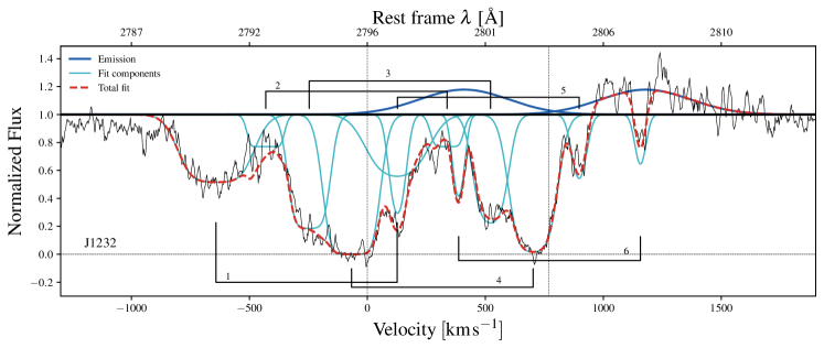
Figure 3 shows an example of the best fit to the Mg II absorption in the galaxy J12320723 (hereafter J1232). The lower horizontal axis shows the velocity of the Mg II2796 doublet component relative to the galaxy systemic redshift (zsys), and the vertical black dotted lines mark the Mg II2796 and Mg II2803 location in the velocity space at zsys, respectively. The Mg II doublet absorption profile is well described by six Gaussian components (shown with light blue solid lines). The brackets in Figure 3 mark Mg II doublet pairs numbered in decreasing order of blueshift velocity from zsys. The three most blueshifted components (1, 2, and 3) are characterized by . Comparison of the Mg II2796 and Mg II2803 trough shapes illustrates their nearly identical intensity, but the lines are not black. The remaining three components have . The spectrum also clearly includes redshifted (410 ) Mg II2803 emission observed up to relative to zsys. (The corresponding Mg II2796 line is not obvious because of Mg II2803 absorption at the same wavelengths.) The inclusion of an emission component in the model significantly improves the fit to the Mg II absorption trough. The red dashed line in Figure 3 represents the total Mg II best fit, including the Mg II emission (dark blue solid line).
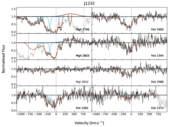
Figure 4 shows an ionic species stack from the spectrum of J1232, centered on the absorption lines included here. Each panel shows the line decomposition (light blue solid lines) and the total best fit (dashed orange lines) to a different ion absorption trough. The light grey part of the spectrum shown in some panels marks a region where multiple transitions overlap in wavelength. The top two left panels show our best fits to Mg II2796 and Mg II2803, respectively. It is worth noting that where the Mg II2796 and Mg II2803 velocity components lie on top of each other, then the dashed orange line does not describe the observed spectrum (in black) because it represents the total fit of a single transition only. For example, the high-velocity Mg II2803 absorption makes the Mg II2796 trough appear to be deeper than the Mg II2803 trough between and . When the best fit profile of both doublet components are combined they fit the data well, as shown in Figure 3 (dashed red line).
3.2.2 Mg I
We also fit Mg I absorption in our sample. Observations of a single Mg I transition do not directly constrain the Mg I2853 optical depth. To quantify the kinematics and absorption strength of Mg I2853 line profiles in our spectra, therefore, we follow two distinct approaches. First, we perform a fit to the Mg I absorption troughs independent from the Mg II fit, as described in Section 3.2. We set = 1 and let the other parameters (i.e. , , and ) vary. This approach assumes that an absorption line that is not black is produced by optically thin gas. If the gas is instead optically thick and the shape of the absorption trough is determined by the this method provides a lower limit to its column density. The Mg I best fit parameters are listed in Table 3 (columns 5, 6, and 7).
Our second approach assumes the optical depth of each Mg I velocity component to be linked to that of the Mg II component. We set and for each Mg I velocity component to be the same as the corresponding Mg II component and estimate what (Mg I) best fits the data. The optical depth in Mg I is
| (4) |
where (Mg I)/(Mg II) is the relative ionization correction. For starburst spectral energy distributions (SED), (Mg II) (Martin et al. 2009). We set the neutral fraction to be 30% (i.e. (Mg I) = 0.3). This approach is motivated by the fact that the Mg I and Mg II absorption troughs have similar kinematic structures, however, Mg I is seen to be shallower than Mg II. When (Mg II) is large and (Mg II) , the neutral Mg fraction must be less than a few percent to produce a shallow Mg I2853 trough with = 1 (i.e. optically thin). In this case, it is more likely that Mg I2853 is optically thick, and the determines the shape of the Mg I absorption trough. We report the results of this approach in Table 3 (columns 2, 3, and 4). We refer to the first approach to the Mg I fit as “independent”, and to the second as “constrained”.
Figure 4 shows an example of our best fit to the Mg I lines in the galaxy J1232. The third from the top left panel shows the best fit to Mg I2853. Following the independent approach, we identify three components falling within and of zsys. They have good kinematic correspondence to three Mg II components, but the Mg I profiles are shallower. In Figure 4 (and for the rest of the sample Figure 5 24) we show the Mg I2853 best fit as derived following the constrained approach. Even in this case, we find that three Mg I velocity components within and of zsys provide a good fit to the data. The three Mg I components are described by values in the range of of (Mg II).
3.2.3 Fe II
The spectral coverage of our data includes a series of strong Fe II resonance lines which have some useful advantages over analysis of the Mg II doublet. First, the large number of Fe II transitions (i.e. Fe II2344Å, Fe II2374Å, Fe II2382Å, Fe II2586Å, and Fe II2600Å) span a wide range of oscillator strengths, which makes it possible to place robust bounds on the column density of singly-ionized iron, thereby better constraining the total gas column density. For example, the Fe II2374 oscillator strength is a tenth that of the strongest transition, Fe II2382Å (which is nearly equal to that of Mg II2803Å). Furthermore, the absorption of Fe II in several of these transitions is followed by fluorescence (rather than resonance) emission, providing a clearer view of the intrinsic absorption profile (Prochaska et al., 2011; Erb et al., 2012; Martin et al., 2012). The Fe II2374Å transition is particularly useful as the resonance absorption trough is not filled in by the emission of fluorescent Fe II2396Å photons.
We quantify the Fe II kinematics for each galaxy in our sample by fitting the absorption line profiles as described in Section 3.2. We model the observed transitions simultaneously to constrain and . At a given velocity relative to zsys, we consider the transitions to have (1) a relative defined by atomic physics (Morton, 2003), and (2) equal and across the transitions. We do not detect any Fe II emission. The Fe II best fit parameters are reported in Table 2. In some spectra we additionally detect and model the Mn II 2576, 2594, and 2606 triplet which can blend with the Fe II 2586, 2600 transitions. The Mn II best fit parameters are also reported in Table 4.
| ID | (Mn II) | (Mn II) | (Mn II) | (Mn II) |
|---|---|---|---|---|
| (1) | (2) | (3) | (4) | (5) |
| J0905 | 0.12 | |||
| J1219 | 0.21 |
Note. — Col 2: Mn II line centroid; Col 3: Mn II covering fraction; Col 4: Mn II Doppler parameter; Col 5: Mn II column density
As Fe II provides a more reliable estimate of the central optical depth, for the velocity components that are detected in both Fe II and Mg II we compare (Mg II) derived from the Mg II fit (as described in Section 3.2.1) with the optical depth inferred from the Fe II fit. We assume a solar abundance ratio, which is supported by an ensemble of line ratio diagnostic diagrams used to estimate the metallicities in our sample (Perrotta et al., 2021). For a solar abundance ratio (log Mg/H = ; Asplund et al., 2021), and conservatively adopting a comparable ionization correction (e.g. (Mg II) (Fe II)), the optical depth in the weaker magnesium doublet line is
| (5) |
While the relative optical depth in Fe II2382 and Mg II2803 can be similar to each other, the Mg II optical depth can be much larger as Fe is more depleted onto dust grains than Mg (Savage & Sembach, 1996; Jenkins, 2009). Since there are not many studies on dust depletion in galactic winds, we adopt dust depletion factors () consistent with those measured in the Galactic ISM (0.5 dex for Mg and 1.0 dex for Fe; Jenkins, 2009). We note that Jones et al. (2018) studied a sample of nine gravitationally lensed star-forming galaxies, and inferred that the outflowing medium is characterized by moderate dust depletion (Fe) = 0.9 dex, in line with our adopted (Fe). Assuming a similar dust depletion correction for Mg and Fe, we would infer a (Mg II2803) that is systematically lower by a factor of three; this would decrease the inferred Mg II column densities (presented below) by roughly a factor of three. Adopting the dust depletion typical of the Galactic halo (0.59 dex for Mg and 0.69 dex for Fe; Savage & Sembach, 1996) would lead to a similar result, with inferred Mg II column densities lower by a factor of 2.3. Hereafter we refer to the Mg II2803 central optical depth derived directly from the Mg II fit as “measured” ((Mg II)meas), and the optical depth deduced using Equation 5 as “inferred” ((Mg II)inf).
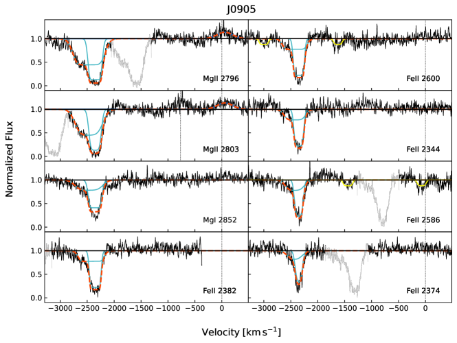
Figure 4 shows an example of our best fit to the Fe II lines in the galaxy J1232. The bottom left and the right column panels show the best fit to the Fe II transitions observed in this study. The shape of the Fe II absorption trough is well described by three kinematic components within and of zsys. Although we do not force agreement in the kinematics of Fe II and Mg II, the different velocity components agree remarkably well (with comparable and to within the errors) over the velocity range where we detect Fe II. We can therefore directly compare their . The three Fe II components all have lower with values in the range of of (Mg II). The (Mg II)meas is not consistent with (Mg II)inf for all the velocity components. From this comparison, we infer that the actual Mg II optical depth is 4 times larger than the minimum required to fit the doublet. The Mg II velocity components detected at and are saturated and the best fit values represent lower limits. For the component detected at 128 , we ascribe the difference as resulting from uncertainties in the emission filling affecting this component.
3.3 Individual Systems
In the sections below we present fits to the Mg II, Mg I, and Fe II absorption lines detected in other three galaxies in our sample, to illustrate the range of line properties observed in our data. Fits for the remaining galaxies are presented in Appendix A. We generally find that the kinematics of Fe II match those of Mg II well, for the components with high EW and SNR.
3.3.1 J0905+5759
Figure 5 shows the best fit to the Mg II, Mg I, and Fe II absorption lines in the galaxy J0905+5759 (hereafter J0905). We present the absorption line fit for this source as an example that exhibits relatively simple kinematics, with few components, and with Mg II2796, 2803 lines that do not blend together. There is strong agreement in the component structure of all the absorption lines. The shape of the Mg II, Mg I, and Fe II troughs are well described by two velocity components spanning to of zsys. The spectrum also displays slightly redshifted ( ) Mg II2796, 2803emission spanning to . However, the resonance emission does not fill in the high-velocity Mg II absorption lines. The comparable intensity at all velocities of the Mg II2796 and Mg II2803 troughs indicates the Mg II is optically thick. As the lines are not black (though the lower velocity component is close to black) the covering fraction () determines the shape of the absorption troughs.
The independent Mg I fit identifies two components with similar kinematics to the constrained fit within the errors. As seen in J1232 above, here the Mg II troughs are deeper than the Mg I troughs, which indicates that only a fraction of the cloud volume contains much neutral Mg. It seems more likely that the Mg I absorption profile shape is determined by rather than optical depth, since the latter (i.e. (Mg I) = 1) would require the Mg neutral fraction to be less than a few percent (see Formula 4). The covering fraction for Mg I is 67 and 40% that of the corresponding Mg II velocity components. Before performing the Fe II fit, we identify and model the Mn II 2576, 2594, and 2606 triplet (yellow solid lines). In this case, they do not blend with the Fe II 2586, 2600 transitions. The Fe II transitions show roughly equal intensities, suggesting they are also tracing optically thick gas. The two Fe II velocity components are not black, and we find they are well described by (Fe II) (90% and 40% of (Mg II), respectively). Based on a comparison of (Mg II)meas and (Mg II)inf, we conclude that the Mg II fit provides only a lower limit on N(Mg II) and that the actual central optical depth for the two Mg II2803 components is closer to 79 and 67 (rather than 6 and 4 as measured from the Mg II fit).
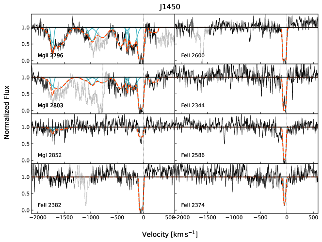
3.3.2 J1450+4621
Figure 6 shows our best fit to the Mg II, Mg I, and Fe II absorption lines in the galaxy J1450+4621 (hereafter J1450). This spectrum exhibits a strong and complex Mg II absorption trough within and of zsys. The Mg II2796 and Mg II2803 line profiles are well described by ten velocity components. Many components (seven in Mg II2796, and five in Mg II2803) blend together. We do not detect Mg II emission in this galaxy. We find that two Mg II components (at and ) are optically thick, and their shape is therefore determined by the covering fraction (= 0.15 and = 0.95). The remaining eight blueshifted components trace optically thin gas with = 1. We detect a strong Fe II absorption line at of zsys, that has good kinematic correspondence to the deepest Mg II component. We model this using only one component and find (Fe II) to be 26% narrower than (Mg II). The absorption trough is black for all Fe II transitions other than Fe II2374. This provides a robust constraint on N(Fe II). Comparing (Mg II)meas and (Mg II)inf for the only component detected in both Mg II and Fe II, we infer that the Mg II fit provides a lower limit on N(Mg II), and the real (Mg II2803) is closer to 74 (than 8, as measured from the Mg II fit). We identify one Mg I absorption trough close to zsys(at ) that is visibly less deep than the corresponding Mg II and Fe II components. The independent and constrained fits agree well in terms of the absorption line kinematics. However, as (Mg II) is at least 8 (and more likely 19), we conclude that the constrained fit provides only an upper limit to N(Mg I) and that the Mg I absorption is tracing optically thick gas (with (Mg I) = 32% (Mg II)). Mg I shows a second weak absorption trough at -1700 that has a good kinematic correspondence to the two most blueshifted Mg II components. We model this using two velocity components and find that the independent fit results in a broader profile than that of the constrained fit. However, the kinematics agree within the errors given the large uncertainties in the independent fit, due to the poor SNR. As the Mg II in these two components traces optically thin gas, we conservatively favor the Mg I independent fit over the constrained fit.
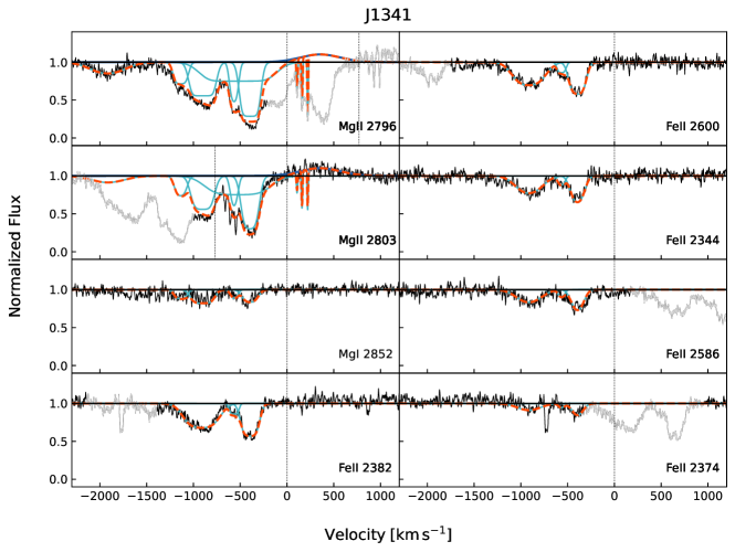
3.3.3 J1341-0321
Figure 7 shows the best fit to the Mg II, Mg I, and Fe II absorption lines in the galaxy J1341-0321 (hereafter J1341). This spectrum includes Mg II redshifted emission ( ) within and of zsys. We detect strong absorption from Mg II falling within and of zsys. We model the Mg II2796 and Mg II2803 troughs using nine velocity components that are characterized by complex kinematics. Most of the components (eight Mg II2796, and six Mg II2803) blend together. The Mg II best fit includes a combination of optically thin (in three components) and optically thick (in five components) gas, and all components have 1. Of note, we identify three extremely narrow redshifted Mg II components. These lines lie on top of the Mg II emission and are not resolved; their best fit parameter is similar to one resolution element (8 ). We detect Mg I and Fe II absorption within and of zsys, which we model using four and three velocity components, respectively. There is strong agreement in the Mg I kinematics of the independent and constrained fit solutions (with comparable and within the errors). The independent fit results in (Mg I) of % of (Mg II). There is a remarkable correspondence between Mg II and Fe II. However, the most blueshifted Fe II component is 57% broader than the corresponding Mg II. We ascribe the difference to the lower SNR in the Fe II spectral region compared to Mg II, which results in fitting Fe II using one component instead of two as for Mg II. We find Fe II to have lower than Mg II ( % of (Mg II)). Based on a comparison of (Mg II)meas and (Mg II)inf, we conclude that the Mg II fit provides only a lower limit on N(Mg II) and that the actual central optical depth for the three Mg II2803 components is closer to 17, 21, and 12 (rather than 4, 1, and 5 as measured from the Mg II fit).
4 Discussion
We detect outflows in 14 compact, massive starburst galaxies in absorption from Mg I, Mg II, and Fe II and show remarkably similar profiles of the absorption troughs in all these transitions. In most of our sample, the velocity dependence of the gas covering fraction () across components defines the absorption trough profile. Similarities in the profiles suggest these species reside in the same low-ionization gas structures. However, Mg II has on average a higher than Fe II at a given velocity, and a higher than neutral Mg, implying that the absorbing clouds or filaments are not homogeneous.
We now discuss our results, including the variation of the absorption line profiles and the possible connection with the star formation history of each galaxy (Section 4.1). In Section 4.2 we examine the lack of substantial absorption at the systemic redshift and the potential effect of emission line filling. We then use our results to gain insights into the role of different physical mechanisms in the extreme galactic outflows observed in our sample (Section 4.3). In Section 4.4 we investigate trends (or lack thereof) between the outflow absorption strength and galaxy properties. We conclude by presenting estimates of the mass outflow rates in our sample and discussing the associated uncertainties as well as the potential for these extreme outflows to affect the evolution of their host galaxies (Section 4.5).
4.1 Variation of Absorption Line Profiles
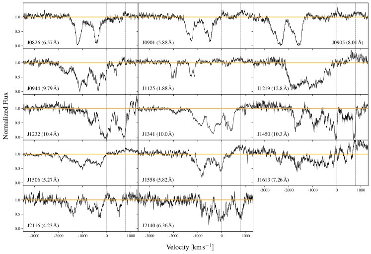
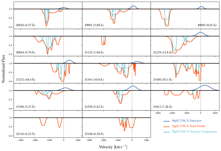
As shown in Section 3.2, each of the galaxies in our sample requires multiple components to fit the absorption troughs for the transitions studied here. The Mg II absorption troughs delineate the outflow kinematics most cleanly. Fig. 8 shows our best fit to the Mg II2796 absorption trough for each galaxy and illustrates the variety of absorption profiles observed in our data.
First, there is a substantial variation in the distribution of the Mg II absorption troughs in velocity space. Two galaxies (J0905 and J1125) lack any absorption from 0 to 2000 . One galaxy (J2116) shows two distinct troughs separated by 600 . Five galaxies (J0826, J0901, J1232, J1558, and J2140) exhibit complex kinematics with contiguous blueshifted absorption from 9001500 . The remaining six galaxies (J0944, J1219, J1341, J1450, J1506, and J1613) have even more complex absorption profiles with nearly continuous blueshifted absorption out to 2000 .
Second, there is a large variation in the number of velocity components required to describe each profile, as well as their widths (or Doppler parameter, ). As discussed in Section 3.2 we fit the blended absorption lines with the minimum number of components needed to characterize the velocity asymmetry. This number varies from two to ten velocity components. Their widths vary from 8 to 344 , with a mean value of 106 . Third, there is a large variation of the Mg II covering fraction () in different galaxies. For four galaxies (J0944, J1450, J1506, and J2140) most of their velocity components have = 1, such that the shape of their absorption profiles is determined by the optical depth rather than . For the rest of the sample, we find as low as 0.12, with a mean value of 0.57. Fourth, three galaxies (J1232, J1341, and J1450) additionally have redshifted velocity components, indicating infalling gas. Lastly, 9 of the 14 galaxies in our sample exhibit clear signs of Mg II emission with velocity shifts from that vary from 0 to . Overall, there is a remarkable variation in the profiles and kinematics of these galaxies.
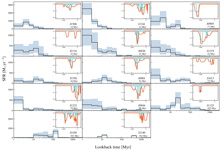
The galaxies in our sample are characterized by extreme and “bursty” star formation episodes that likely drive the powerful outflows observed, which can reach far into the circumgalactic medium (CGM) of the galaxy (Rupke et al., 2019). As mentioned in Section 1 our team observed the galaxy Makani with the Keck CosmicWeb Imager (KCWI; Morrissey et al. 2018) and uncovered two distinct outflows traced by [OII] emission: a larger-scale, slower outflow (300 ) and a smaller-scale, faster outflow (1500 ). The velocities and sizes of the two wind components map exactly to two recent starburst episodes that this galaxy experienced 0.4 Gyr and 7 Myr ago, determined by its star formation history (SFH). To understand if the Mg II multiple velocity components seen here in this larger sample are also connected to the highly impulsive “burstiness” of the star formation in these galaxies we next investigate potential correlations between the Mg II absorption profiles and the SFHs of each source.
Figure 9 shows the SFHs for the galaxies in our sample derived using Prospector (Johnson et al., 2021) as described in Section 2.2. The mean light-weighted age of the stellar population younger than 1 Gyr is reported in the bottom right of each panel. The Mg II2796 absorption profile model is shown for each target in the upper right inset as presented in Fig. 8. We note that the order of the galaxies in this figure is different from the others in the paper and follows their light weighted age.
Unlike Makani which had two clear bursts and two clear outflows at different velocities, we do not find a simple correspondence between the number of bursts in the SFH and the number of Mg II absorption features in this study. Galaxies exhibiting similar Mg II absorption troughs can have a variety of SFHs and vice-versa. For example, the Mg II EWs of J0905 and J1125 are substantially different, 8.01 and 1.88 Å, respectively. However, their absorption troughs are similar in several regards as they both show no absorption from 0 to 2000 and are fit using two velocity components. Their SFHs both display a burst of star formation around 30 Myr ago, but their light-weighted ages are substantially different (17 and 102 Myr, respectively) as J0905’s SFH is characterized by a younger burst 6 Myr ago. As another example, J1341 and J1450 have comparable Mg II EWs (10 and 10.3 Å) and very broad blueshifted troughs (2000 ) with extremely complex kinematics fit with a close number of components (nine and ten). Nevertheless, they have SFHs that are substantially different, with inferred light-weighted ages of 14 and 107 Myr, respectively. In particular, J1341 shows a starburst in the last 10 Myr, as opposed to J1450 which has no significant bursts in the same time frame. On the other hand, J0826 has a SFH that is similar to J1341; however J0826 exhibits a remarkably different Mg II absorption trough, with a narrower profile (1500 ), no absorption at the systemic redshift (zsys), no redshifted components, and a minimum absorption at a much higher velocity of . Additionally, J0901 has a Mg II absorption profile that is comparable to J0826 in shape and EW but has a very different SFH, with older light-weighted age (54 Myr) and a decreasing trend of star formation in the last 10 Myr.
The galaxies with the fastest velocity components are not necessarily the ones with the most recent bursts, and the galaxies with strong recent bursts do not all have fast outflow components, though some do (e.g. J0826, J0905, J0944, J1219, J1341, J1613). Furthermore, we do find that eight galaxies (J0826, J0901, J0905, J1125, J1450, J1558, J1613, and J2116) have in their SFH an older burst (10 Myr ago), regardless of the presence of a younger burst. Among these 8 galaxies, 6 (all except J0905 and J1125) have Mg II components at low velocities that may be tracing slower outflowing gas driven by the older burst of star formation, similarly to Makani.
4.2 Absorption and Emission at the Systemic Redshift
The Mg II doublet is the most sensitive transition among the absorption lines covered in this study, however, it is affected by resonantly-scattered wind emission which we expect to fill in the absorption profiles around zsys (Martin et al., 2012; Prochaska et al., 2011). As Mg II is a resonant transition, the emitted photons are continually reabsorbed due to the absence of fine-structure splitting. This trapping process interferes with the escape of the photons, complicating the interpretation of the origin of Mg II emission. In the traditional model of a galactic-scale outflow expanding as a shell, this creates a P-Cygni-like profile for each Mg II doublet component, with blueshifted absorption and redshifted emission. The Mg II absorption arises from gas moving toward the observer as it absorbs photons in its rest frame. The emission arises from the receding component of the outflow, where photons emitted in the rest-frame, having scattered to escape towards the observer, are redshifted and go through any intervening gas. The emission line profile is centered near the systemic redshift of the galaxy. This emission can “fill in” the absorption within 200 of zsys, decreasing the EW by up to 50%, shifting the centroid of the absorption lines by tens of , and reducing the opacity near systemic. A study of cool gas outflows that ignores this line emission may underestimate the true optical depth and/or incorrectly infer that the wind partially covers the source (Prochaska et al., 2011).
In our sample, we detect Mg II emission in 9/14 of the galaxies, with velocity shifts of 0 to from . In J0905 we can observe emission in both Mg II lines, with an observed ratio of 1. This ratio is in the optically thick regime (e.g. Chisholm et al., 2020), and it agrees with the ratio observed in Makani (Rupke et al., 2019). The Mg II trough in J0905 is so blueshifted ( ) that the Mg II absorption profile is not affected by emission filling. For the remaining eight galaxies we adopt a ratio of 1 in our fits, as they clearly show Mg II2803 emission but the corresponding Mg II2796 line is suppressed by Mg II2803 absorption at the same wavelengths. If the ratio of the two Mg II components is closer to 2 rather than 1 we may underestimate the effect of line-filling. However, the Mg II absorption profiles in these galaxies are not substantially affected by emission filling as the resonance emission is not expected to fill in the high velocity components of Mg II absorption.
In our sample the majority of the Mg II absorption EW is blueshifted; the minimum intensity of the trough lies near the systemic velocity in only two objects (J1450 and J1232). The intensity minima are blueshifted by 300 to 2,000 in the rest of the sample, with little or no absorption at the systemic velocity. We use the Mg II2803 absorption profile to quantify the EW at systemic, as it does not suffer from blending with Mg II2796. We find that 11/14 galaxies in our sample have less than four percent of the Mg II EW within 200 of zsys. Among the objects that display Mg II emission, J1232 is the most potentially affected by emission filling as 26% of its Mg II EW is within 200 of zsys. However, emission filling is not a concern for the bulk of our sample of highly blueshifted Mg II absorption lines.
The lack of substantial Mg II absorption at the systemic velocity is an interesting feature in our sample, as first noted in Perrotta et al., 2021 and Davis et al., (submitted). One interpretation of the lack of absorption at systemic could be that the extreme outflows in these galaxies may have expelled the bulk of the interstellar medium (ISM) in these sources. However, as many of the galaxies in our sample had a burst of star formation in the last 10 Myr, it is unlikely that these recent winds have entirely removed the ISM on such a short time scale. Additionally, some galaxies likely have ongoing star formation, such that the ISM can not be entirely absent.
Another possibility is that the lack of absorption at systemic is due to an observational selection effect. Our parent sample is characterized by an extremely high outflow detection rate (90%; Davis et al., (submitted)). While it is possible that this high outflow incidence reflects a very wide opening angle of ubiquitous outflows in these galaxies, it could also be that the magnitude and color cuts used to select our sample may have identified galaxies where a powerful outflow has excavated a hole in the ISM, causing the galaxies to appear very bright and blue. As a consequence, there may be little or no ISM left along the particular lines of sight studied here, while there is still remaining ISM in the galaxies along other sightlines.
An example of this scenario is provided by the galaxy J0905. Geach et al. (2014) use the IRAM Plateau de Bure interferometer to study the CO(2-1) emission line in J0905, which is a tracer of the bulk of the cold molecular gas reservoir. They observe a CO emission line at the systemic velocity of the galaxy, which traces 65% of the total cold molecular gas in the galaxy with an inferred mass of . This suggests that along some sightlines the amount of gas swept up by the outflow can be large, despite the galaxy retaining a substantial amount of its ISM.
Another potential explanation for the exceptionally high velocity Mg II absorption components and the lack of absorption at zsys is provided by strong radiative cooling (e.g., Bustard et al., 2016; Thompson et al., 2016). It is possible for a cold gas phase to form “in-situ” within a large-scale galactic wind via thermal instabilities and condensation of a fast-moving hot wind rather than being entrained and gradually accelerated. The by-product of this mechanism is cold gas at similar high velocities as the hot phase. In this model, the cold clouds accelerated by the hot wind are rapidly destroyed on small scales and at low velocities by hydrodynamical instabilities. As a result, the hot wind with enhanced mass loading and density perturbations can cool radiatively on larger scales forming an extended region of atomic and ionized gas moving at 103 , while the gas at low velocities is not observable. We come back to the origin and formation of cold gas in galactic outflows in the next Section 4.3.
4.3 Comparison with Theoretical Models
The existence of very fast, cool gas observed in outflowing winds from star-forming galaxies has been a persistent puzzle. In this Section, first, we briefly describe the processes most commonly invoked for cool gas acceleration in winds, then we use the results from this study and our parent sample to understand what insights can be gained into the role of these mechanisms in the extreme galactic outflows observed here.
4.3.1 Mechanisms of Cool Gas Acceleration
The cool gas phase in winds is commonly explained as the acceleration of clouds from the host ISM via ram pressure from the hot phase (e.g., Veilleux et al., 2005). However, several simulations have challenged this explanation, demonstrating that ram pressure alone is not effective at accelerating cool gas clouds to the velocities and large scales observed without the clouds being shredded by hydrodynamical instabilities and becoming incorporated into the hot flow (Cooper et al., 2009; McCourt et al., 2015; Scannapieco & Brüggen, 2015; Schneider & Robertson, 2015, 2017; Zhang et al., 2017). Recent work has shown that under the right background conditions and when sufficient large clouds are considered, cool gas can survive as a result of a mixing and cooling cycle. This may increase the cool gas flux as the hot gas condenses out, effectively growing the clouds rather than destroying them (Armillotta et al., 2016; Gritton et al., 2017; Gronke & Oh, 2018, 2020; Fielding & Bryan, 2022).
In an alternative model (Efstathiou et al., 2000; Silich et al., 2003; Thompson et al., 2016) the cold phase can form “in-situ” via thermal instabilities and condensation from the hot wind on large scales, provided it is sufficiently mass-loaded via the destruction of cool gas in the inner regions of the flow (see also Lochhaas et al., 2018). Additional models for cold cloud acceleration have also been proposed including momentum deposition by supernovae, the radiation pressure of starlight on dust grains (Murray et al., 2005, 2010, 2011; Hopkins et al., 2012; Zhang & Thompson, 2012; Krumholz & Thompson, 2013; Davis et al., 2014; Thompson & Krumholz, 2016), and cosmic rays (Everett et al., 2008; Socrates et al., 2008; Uhlig et al., 2012). It has also been suggested that several of these mechanisms may be taking place simultaneously in order to drive cool outflows efficiently (Hopkins et al., 2012; Veilleux et al., 2020), making it difficult to isolate the different processes potentially at play.
From an energetic point of view, starburst galaxies with powerful winds, like those in our sample, are ideal candidates for outflows driven by the radiation pressure from Eddington-limited star formation (Diamond-Stanic et al., 2012; Geach et al., 2014; Rupke et al., 2019; Perrotta et al., 2021). Recently, our team obtained results that confirm this hypothesis. Rupke et al., (submitted) present Keck/ESI (Echellette Spectrograph and Imager; Sheinis et al., 2002) long-slit spectra of the two wind episodes observed in the galaxy Makani, drawn from the same parent sample as the galaxies in this study. They infer momentum and energy outflow rates in the inner ( kpc), recent (7 Myr ago), fast (2,000 ) outflow that implies a momentum-driven flow driven by the hot ejecta and radiation pressure from the extreme, possibly Eddington-limited, compact starburst.
Here, in the Sections below, we focus on the kinematics of low-ionization absorbers tracing the cool, ionized phase of the extreme outflows in our sample to gain insights into the distribution of the outflowing gas and the physical mechanisms that may occur at the interface between the hot and cool wind phases.
4.3.2 Inferred Spatial Distribution of Ionized Gas
Simulations indicate that halos of Mg II emission are a ubiquitous feature across the galaxy population to at least z = 2 (Nelson et al., 2021). Mg II halos extend from a few to tens of kpc at the highest masses, i.e. far beyond the stellar component of a galaxy. Moreover, they are highly structured, clumpy, and asymmetric. DeFelippis et al. (2021) generate mock Mg II observations from the TNG50 simulation (Nelson et al., 2021) and produce absorption spectra to compare with observed data. Although the mock sight lines are too small to be comparable with observations, they show the non-uniform distribution of the Mg II absorption, usually concentrated in discrete clumps. The mock velocity spectra, despite originating from a remarkably small fraction of the total Mg II gas in the halo, reflect the diversity of the Mg II gas distribution and kinematics in halos of similar galaxy mass. On the other hand, halos with similar morphology exhibit similar mock spectra. The sample of star-forming galaxies in DeFelippis et al. (2021) differs from ours as it is characterized by galactic disks, while our galaxies are late-stage mergers with spherical morphologies. However, we also find great diversity in the Mg II absorption profiles (see Section 4.1). This suggests that the Mg II halos of our galaxies, despite spanning only 0.76 dex in stellar mass, may have diverse morphologies.
Mg II absorption traces cool 104 K gas that is usually found in simulations in high-density clouds or filaments permeating the volume-filling, low-density, hot phase at large radii (Schneider et al., 2020; Nelson et al., 2021). The remarkably extended velocity distribution of the Mg II absorption profiles in our sample may reflect the filamentary structure of dense outflowing material. Additionally, some simulated halos exhibit fountain flows in Mg II emitting gas, with signatures of infalling gas clouds in addition to wind-driven outflows (Nelson et al., 2021). We note that we find clear signatures of inflowing gas in the spectra of three galaxies in our sample (J1232, J1341, and J1450), where the components that trace infalling gas are redshifted 200300 (from the systemic redshift) and are notably narrower that the blueshifted components that trace outflowing gas. Studies of infalling gas typically utilize surveys of a hundred or more galaxies, as the detection rate of redshifted absorption lines is around 36% (e.g. Sato et al., 2009; Martin et al., 2012; Rubin et al., 2012). The fraction of galaxies with inflows in our sample is 2111%, higher than in other studies. However, this value is based only on three sources, so we can not conclusively state whether the accretion rate in our sample is significantly higher.
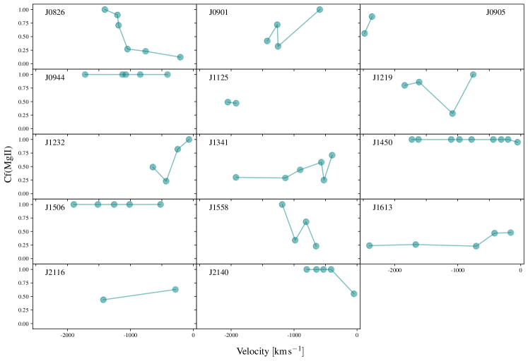
Simulations showing the survival of cool clouds traveling through a hot medium find that the clouds undergo hydrodynamical instabilities that create an elongated shape with a wake (e.g., Armillotta et al., 2016; Gronke & Oh, 2018). The coolest and densest gas is typically located inside the head of the cloud, while the ionized gas is found more in the turbulent wake behind the cloud, produced by the mixing between the cool gas ablated from the cloud and the hot medium. One way to investigate this potential structure observationally is to compare the absorption troughs of two transitions of the same species that have different ionization, such as neutral and singly-ionized Mg. As mentioned in Section 3.2.2, one of our approaches to fit Mg I absorption profiles is to adopt the same kinematic components as Mg II and estimate the covering fraction () that best fits the Mg I spectral region. An advantage of constraining the kinematics in this way is that we can directly compare the of the two different ions as a function of velocity. We find that the shallow troughs of Mg I relative to Mg II require a lower for the former at every velocity, with (Mg I) ranging from to (Mg II), with a median value of (Mg I) = 0.4 (Mg II). The similar kinematics but systematic offset in implies that the Mg I absorption arises from denser regions within more extended structures traced by Mg II. This finding is in agreement with theoretical models predictions that the coolest and densest gas is typically located in the more internal and self-shielded part of the clouds.
We note that even if we do not adopt the same kinematics for Mg II and Fe II, we find a remarkable agreement in most of the velocity components. For these components, we find that (Fe II) is systematically lower than (Mg II). This is expected as Fe II traces denser gas than Mg II, and it is in line with the previous result of Mg I being less spatially extended than Mg II.
4.3.3 Covering Fraction Trends with Outflow Velocity
Earlier studies have tried to interpret line profiles of low-ionization ions (e.g. Mg II, Mg I, Fe II), and in particular their distribution, in the context of driving mechanism models for galactic winds. Martin & Bouché (2009) study a sample of five starburst galaxies at z0.2 and find that decreases as the outflow velocity increases beyond the velocity of minimum intensity, which in their case corresponds to the velocity of maximum . The authors interpret the velocity-dependent in their sample as a result of geometric dilution associated with the spherical expansion of a population of absorbers. In the context of this simple physical scenario, their result implies that the high-velocity gas detected in absorption is at a larger radii than the lower velocity (and higher ) gas, implying an accelerating wind. This hypothesis is also suggested by Chisholm et al. (2016) in a study of the wind-driving mechanisms and distribution of in a nearby starburst galaxy. This simple accelerating model does not take into account, however, the complexity of the interaction between cool clouds and the hot surrounding wind, such as radiative cooling, cloud compression due to shocks, and effects of shear flow interactions that produce hydrodynamic instabilities. More recent studies have shown that cold clouds are unlikely to survive that kind of acceleration over time (Scannapieco & Brüggen, 2015; Brüggen & Scannapieco, 2016; Schneider & Robertson, 2017; Zhang et al., 2017).
Figure 10 shows the fitted Mg II() as a function of velocity for the blueshifted (i.e. outflowing) components in our sample. does not show a unique trend with velocity. Seven galaxies (J0901, J0905, J1219, J1232, J1341, J1613, and J2116) have decreasing with increasing velocity, three galaxies (J0826, J1125, and J1558) have increasing with increasing velocity, and four galaxies (J0944, J1450, J1506, and J2140) have a constant value. This variation in the with outflow velocity, along with the variation of the absorption profiles described in Section 4.1, may capture the complex morphology of kpc scale, inhomogeneously distributed, clumpy gas and the intricacy of the material in the turbulent mixing layers between the cold and the hot phases (e.g., Fielding et al., 2020; Nelson et al., 2021).
Our starburst galaxy sample shows that a model of an outflow accelerating over time is unlikely to be valid. One piece of evidence is the observation of the large scale, multi-phase, and multi-burst wind in the galaxy Makani. Rupke et al. (2019) find that the inner ( kpc) and younger (7 Myr ago) wind is faster (with maximum speeds exceeding 2000 ) than the more extended ( kpc) and older wind (400 Myr ago), which has speeds of 100 . Rupke et al. (submitted) find that the larger wind is consistent with having slowed down in the extended halo and CGM of the galaxy.
A second piece of evidence against an accelerating model comes from the analysis of the Mg II EW and velocity as a function of the light-weighted age of the galaxies in our parent sample. In this work, we do not find a correlation between the total Mg II EW and galaxy light-weighted age. However, the galaxies all have young light-weighted ages, between 13 and 192 Myr, and represent many of the youngest objects in the parent sample studied by our team (Davis et al., (submitted)). Using the parent HizEA sample, which has a larger dynamic range in light-weighted age, Davis et al. (in prep) find an inverse correlation between Mg II absorption EW and light-weighted age, as well as a complementary inverse correlation between outflow velocity and light-weighted age. These results are consistent with models in which the outflow decelerates with time, which support scenarios in which the cold gas condenses out of a hot flow. In particular, the observed trend of lower outflow velocity with larger light-weighted age matches the analytic models of Lochhaas et al. (2018) well, where impulsive bursts of star formation driven winds slow down and cool as they expand into the CGM.
Regardless of their physical origin, the large velocity width of the absorption troughs observed here requires contributions from multiple structures along the sightline. It is likely that our sightlines intersect many mixing layers, making it difficult to interpret the inferred from our fits in terms of the of single clouds that grow over time entrained in the hot wind (e.g., Gronke & Oh, 2018; Fielding & Bryan, 2022). To complicate the interpretation of the absorption line profiles further there is the multi-burst nature of the outflows in our sample. It is possible that an initial burst of star formation drives an outflow that consumes most of its energy shock-heating the surrounding ISM and consequently slows down while excavating a hole through which we observe the host galaxy as blue and bright. An outflow driven by a second burst of star formation may have a very different evolution as it can follow the path of minimum density and inertia created by the first burst, retaining more energy and velocity. A single sightline does not provide a full picture of the entire galaxy, and it can intersect multiple outflow episodes, which can overlap in the projected observed velocity space, making it challenging to distinguish the two wind episodes through absorption studies.
4.3.4 Comparison of MgII and FeII Absorption Troughs
It is currently challenging to use simulations to interpret observed absorption line profiles, as the models do not typically create spectra drawn from realistic sightlines through the simulated halos. They also typically identify the cool wind phase by temperature rather than making predictions for individual ions. However, we can consider their main results and model trends to make comparisons with observed spectra.
Schneider et al. (2020) present a new simulation part of the Cholla Galactic OutfLow Simulations (CGOLS) project, a series of high-resolution global disk simulations of galaxy outflows. The authors model an M82-like galaxy with a 5 pc resolution in a 10 kpc volume, which is ideally suited to capture both the launching of the wind and the detailed phase structure during the subsequent expansion. Their stellar feedback injection mechanism allows the driving of energetic hot winds from a high surface density galaxy disk that gives rise to a complex, multiphase outflow. They find that the cold phase is primarily in embedded clouds that are gradually shredded and thereby enhance the mass loading of the hot phase. The authors demonstrate that the mixing between hot and cool gas in the wind is an effective way of transferring momentum from one phase to another, and this occurs at all radii. In cases where the mixed gas has a high enough density to cool, it does so with a higher velocity, leading to a linear relationship between mixed fraction and velocity.
To test this prediction we can assume that the Fe II in our spectra primarily traces the entrained cool gas phase component (i.e., gas rich in Fe results from SN Ia explosions), while the Mg II primarily traces the cooled hot wind material (i.e., gas ejected from SN II and rich in -elements). As we do not expect the hot wind to be composed entirely of SN II ejecta, it should be -element enriched but quite diluted compared to pure SNe ejecta. Therefore rather than searching for a complete absence of Fe II, we can instead examine how the Mg II to Fe II ratio varies as a function of outflow velocity. We expect the EW(Mg II) to EW(Fe II) ratio to increase for gas with less mixing (i.e., with less cool gas entrained as the hot wind travels through the ISM); such gas likely originates from direct cooling of the hot wind phase.
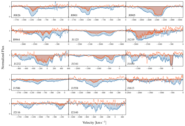
In Figure 11 we overlay the Mg II2796 (blue spectrum) and Fe II 2382 (red spectrum) absorption profiles for the galaxies in our sample. We find that the Mg II2796 troughs typically have higher absorption EW. Eight galaxies (J0826, J1232, J1341, J1450, J1506, J1558, J2116, and J2140) exhibit a clear lack of Fe II at the highest velocities. To verify that this lack of Fe II is not due to a sensitivity effect, we use Equation 5 to infer the Fe II optical depth for the velocity components where Fe II is not detected. For each component, we use the optical depth of the corresponding Mg II and assume Mg II and Fe II to have the same kinematics. Equation 5 takes into account the difference in oscillator strength and dust depletion between Fe II and Mg II. As Fe II typically has lower compared to Mg II, we adopt a lower (Fe II), in line with the other Fe II absorption lines in the same spectrum. We find that in four of these galaxies (J0826, J1341, J1506, and J1558) we can not exclude that Fe II absorption may be present but too weak to detect. In the other four galaxies (J1232, J1450, J2116, and J2140) the lack of Fe II at the highest velocities is real and can be explained by gas cooling directly from the hot wind at the highest velocities. We also find that in two galaxies (J0944, J1613) there is a lack of Fe II at the lowest velocities that is not due to sensitivity effects. Finally, J2140 is the only galaxy in our sample where Fe II is not detected at any velocity. This is also the only galaxy in our sample that hosts a faint AGN (Sell et al., 2014), which could result in different feedback mechanisms and spectral features.
In Figure 12 we show the Mg II2796 to Fe II 2382 EW ratio as function of outflow velocity. To calculate this ratio we divide the Mg II2796 (corrected for Mg II2803 absorption) and Fe II 2382 spectral regions in bins of 200 and integrate the spectra, in order to estimate upper limits where the lines are not detected. The size of the circles in this figure is proportional to the strength of the EW(Mg II). Filled circles show the velocity bins where we detect Fe II, while empty circles show Fe II non-detections. This EW ratio does not have a consistent trend with the outflow velocity. However, for the eight galaxies discussed above that lack Fe II at the highest velocities, the EW ratio is larger than in the velocity bins where we detect Fe II.
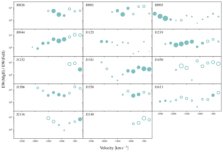
In summary, several of the galaxies in our sample do not have Fe II detected at the highest outflow velocities, implying a lower mixing fraction of entrained cool gas. While the cold gas outflow phase is most likely produced by a combination of physical mechanisms, these results suggest that the cold gas at the highest velocities could directly condense out of the hot wind phase, as suggested by some theoretical models.
4.4 Trends of Equivalent Width with Galaxy Properties
We now investigate the relationship between the outflow absorption strength and galaxy properties in our sample. Figure 13 compares the total Mg II equivalent width (EW) with host galaxy stellar mass (M∗), star formation rate (SFR), and star formation rate surface density (). Since the Mg II doublet components are blended together in most of our galaxy spectra, we consider the total EW measured from the Mg II2796, 2803 transitions. We compare our sources with data from five representative star-forming galaxy samples in the literature that provide information about both Mg II doublet component EWs (Weiner et al., 2009; Kornei et al., 2012; Rubin et al., 2014; Bordoloi et al., 2014; Prusinski et al., 2021).
To quantify the relations presented in Figure 13, we use the python Markov Chain Monte Carlo package PyMC3 (Salvatier et al., 2016) to compute a linear fit and the associated uncertainties. In each panel, we show the linear fits with 1 and 3 error regions shaded in blue. We also characterize the correlations using the Spearman rank correlation coefficient () and the Pearson linear correlation coefficient (). These values and their corresponding statistical significance are listed in the figure caption.
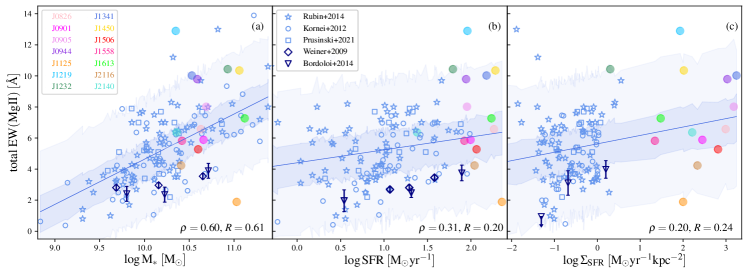
A strong positive correlation between EW(Mg II) and M∗ is evident in panel (a) of Figure 13, while EW(Mg II) exhibits a weaker correlation with SFR in panel (b) and in panel (c), as has been found in previous work (e.g., Martin et al., 2012; Rubin et al., 2014). Our galaxies follow the general trends seen in other samples, though with substantial scatter. The EW(Mg II) versus M∗ correlation has been explained in these previous works as being due to two factors: 1) the EW of ISM absorption (at the systemic redshift) increases with increasing M∗, and 2) emission filling is stronger in lower mass galaxies, preferentially suppressing absorption around the systemic redshift. As a result, the lower emission filling in the spectra of massive galaxies (relative to lower mass galaxies) amplifies the positive correlation between EW(Mg II) and M∗.
As described in Section 4.2, our sample of massive galaxies lacks substantial ISM absorption at the systemic velocity, and the large EWs(Mg II) observed here are typically from absorption that is blueshifted more than 200 , such that emission filling is not substantial. The systematically larger EWs of massive galaxies may be due to a larger number of blueshifted components compared to lower mass galaxies, which would imply a correlation between the maximum velocity of the outflows and M∗. This has been observed (e.g., Davis et al., submitted, Rubin et al., 2014; Heckman & Borthakur, 2016), though the correlation with stellar mass does not appear to be as strong as with other galaxy properties. Therefore, the explanation previously proposed for the EW(Mg II) vs. M∗ correlation is plausible.
Another potential contributing factor to the EW(Mg II) vs. M∗ correlation is that as M∗ increases, the reservoir of gas that can potentially be part of the outflow should increase as well, for star-forming galaxies. In this context, the mass and velocity of the outflowing gas are consequences of the star formation conditions in the galaxy. There is growing agreement that is one of the most important properties governing the velocities of galactic winds (e.g., Davis et al., submitted, Heckman et al., 2015; Heckman & Borthakur, 2016; Prusinski et al., 2021). If we consider two galaxies with similar EW(Mg II), M∗, and SFR but different , we may expect the galaxy with higher to have a higher outflow velocity, as the similar energy released by the supernovae explosion is injected into a smaller volume creating a more explosive event. We see this trend if we consider the most massive starburst galaxies from Rubin et al. (2014) and Kornei et al. (2012) with EW(Mg II), M∗, and SFR comparable to our sample. The 2 dex larger in our sample is reflected in the substantially higher outflow velocities observed (Davis et al., submitted). A specific example is J1232, which has similar to the most massive galaxies from Rubin et al. (2014) and Kornei et al. (2012) and it also has a comparable outflow velocity v98 = 761 (vavg = 217 ), which is the lowest in our sample. In this context, considering two galaxies with similar M∗, SFR, and but very different EW(Mg II), we may expect that the galaxy with lower EW(Mg II) would have a higher outflow velocity, as a comparable amount of energy injected has to accelerate less gas. An example of this is J1125, which has similar M∗, SFR, and to J1450, but has 5 times lower EW(Mg II) and a substantially larger outflow velocity of v98 = 2244 (vavg = 1813 ), compared to v98 = 1874 (vavg = 529 ) for J1450.
While the general trends described above apply to many galaxies in Figure 13, there are exceptions, and these relations have substantial scatter. While such scaling relations are not trivial to interpret, they can be useful from a statistical standpoint. However, when we look at the details of individual galaxies, such general trends may not strictly apply, especially given that single sightlines can provide only a partial view of the entire galaxy. Another complication is that EWs measured from saturated absorption lines reflect only a lower limit on the wind absorption strength.
4.5 Mass Outflow Rates
In this section, we estimate mass outflow rates for the observed winds in these galaxies and discuss the assumptions used to determine these values. We note that the mass outflow rates are confined to the phase we probe with our observations, which is the ionized gas phase, and therefore they are lower limits on the total mass outflow rates which include neutral and molecular gas (e.g. Bolatto et al., 2013; Chisholm et al., 2016).
Following Rupke et al. (2005b) we assume a simple model for the wind that depends on the physical parameters derived from our line fitting. If we consider a single thin shell wind at radius , with thickness , the average mass outflow rate is:
| (6) |
where is the mean atomic weight ( is the proton mass and = 1.4 is the correction for the relative He abundance). We calculate time-averaged outflow rates because they are a more useful quantity than instantaneous values to use when comparing to star formation rates. To average the mass outflow rate over the wind lifetime and obtain Equation 6, we divide the instantaneous by .
The sum in Equation 6 is performed over the individual outflowing (i.e., blueshifted) velocity components in each galaxy: is the solid angle subtended by a given component as seen from the wind’s origin, (H) is the total hydrogen column density of that component, and is the central velocity of that component. In this model, we split (the wind’s global covering factor) into two parts to account for a potential biconical morphology and a clumpy wind, rather than assuming a smooth shell. We model in terms of the large-scale covering factor , related to the wind’s opening angle, and the local covering factor , related to the wind’s clumpiness. Thus, . We adopt based on the high outflow detection rate in the parent sample (Davis et al., (submitted)). We can then rewrite Equation 6 as
| (7) |
An estimate of the total hydrogen column density in the outflow requires knowledge of the ionization state and metallicity of the gas, as well as the amount of dust depletion for the element employed to derive (H). Our spectral coverage provides access to a series of strong Fe II resonance lines which have oscillator strengths spanning a substantial range and therefore can be used to estimate the column density of singly ionized iron. From this one can determine the total hydrogen column density for an assumed metallicity and ionization fraction. However, as we detect Mg II in a larger number of absorption components for most galaxies in our sample, we begin with estimates of the total hydrogen column derived from Mg II. We describe below how these values might need to be adjusted to provide more accurate estimates using results from Fe II where they exist.
We adopt (Mg II) = 0.7 since, in the case of Mg, the singly-ionized state Mg II is likely dominant in photoionized gas at 10 (Murray et al., 2007; Churchill et al., 2003). We assume a solar abundance ratio (log Mg/H = ; Asplund et al., 2021), which is consistent with results from an ensemble of line ratio diagnostic diagrams used to estimate the metallicities of galaxies in our sample (Perrotta et al., 2021). We assume a dust depletion factor (d(Mg)) of dex for Mg, as measured in the local Galactic ISM (Jenkins, 2009). The total hydrogen column density in the outflow is
| (8) |
where the sum is performed over the individual Mg II outflowing velocity components in each galaxy. We list in Table 2 the (H) values derived using this method. These values are lower limits not only because of our assumed conservative ionization correction, dust depletion, and abundance ratios but also because the absorption in the Mg II components is saturated for most of the galaxies in our sample. We emphasize that most of the saturated Mg II absorption troughs in our spectra do not appear black which implies that 1.
Because the actual hydrogen column densities could be substantially higher than those estimated above from Mg II, we can use bounds on (Mg II) from Equation 5 to obtain a revised (Mg II) for all the Mg II components that are also detected in Fe II. Using these values, we derive updated (H) that we report in Table 2. In our galaxy sample the hydrogen column density for the same component obtained from Equation 8 using (Mg II)meas (i.e. measured directly from Mg II fits) and (Mg II)inf (i.e. inferred using bounds from Fe II fits) differ from a factor ranging from 0.3 to 19. The total hydrogen column density for each galaxy is obtained as the sum of (H) for the individual velocity components. Using the highest (H) values in Table 2 (i.e., obtained using , or ), we obtain total hydrogen outflowing column densities for our galaxies of (H)tot = 3 2 , with a median column density of 2 . For most galaxies in our sample, these values are still lower limits, as Fe II provides a bound on only for 36% of the Mg II absorption troughs in our sample. Moreover, our estimates are derived assuming a conservative depletion of iron (relative to magnesium) onto dust grains. Dust depletion factors () measured in the local Galactic ISM fall in the range dex for Fe (Jenkins, 2009). Here we adopt (Fe) = dex; a greater depletion correction would increase (Mg II)meas, and consequently (H), by a factor of . There is therefore an order of magnitude uncertainty due to the dust depletion correction alone.
Returning to our goal of estimating the mass outflow rates in the winds observed in absorption, we can use the values constrained by our fits for all of the variables in Equation 7 except for the spatial extent of the wind (). While the absorption lines are sensitive to absorbing gas at any location along the line of sight to the observed galaxies, they do not provide information on the outflow geometry. Here we choose to adopt a thin shell of uniform radius 5 kpc. This radius is motivated both by observations of star-forming galaxies at similar redshifts (e.g., Burchett et al., 2021; Zabl et al., 2021) and by our own integral field spectrograph data of outflows observed in our sources (Rupke et al., 2019). Rupke et al. (2019) use KCWI to map the [O II] and Mg II emission in the galaxy Makani. They detect resolved Mg II emission on scales 15 kpc. While this galaxy represents an exceptional object with the largest [O II] nebulae ever observed, our team has collected KCWI observations for an additional 13 sources and uncovered [O II] and Mg II nebulae reaching far beyond the stars in the galaxies, with radial extents of a few tens of kpc (Perrotta et al. in prep). Therefore, a physical extent of 5 kpc for the outflows in this paper is used as a reasonable order of magnitude estimate. Determining a more accurate value is challenging as these galaxies show variations object to object and ion to ion. Since is directly proportional to , any change in the physical extent of the outflow will proportionally result in a change to . For example, if the value of increases by a factor of two, will increase by a factor of two. Assuming a thick wind instead of a thin wind will decrease the derived outflow rates since the radial factor in Equation 7 is the inner radius in the thick wind case, rather than the outer radius. For example, a thick wind extending from 1 to 5 kpc has a mass 5 times lower than the kpc thin shell that we adopt here. We prefer a shell geometry over a constant velocity wind given the morphology of the ionized outflow observed in Makani that resembles an evacuated and limb-brightened bipolar bubble. Moreover, a constant velocity wind is likely not appropriate for our sample, which has had recent strong star formation bursts due to major merger activity. Finally, the absorption spectra presented here do not support a constant wind velocity model given their multi-component nature and large velocity extent. We emphasize that while the geometry of the outflow (e.g., physical extent, thickness) is uncertain, this is subdominant to other uncertainties such as the dust depletion factor and optical depth, as discussed above. We may rewrite Equation 7 using fiducial values as follows:
The values for our sample derived using Equation 7 are reported in Table 5. The values obtained using constraints only from Mg II fits are listed in column 1, while column 2 lists calculated utilizing constraints from Mg II and, when available, Fe II fits. We have robust estimates (i.e., non lower-limits) on the ionized gas column density for only two sources in our sample, J0905 and J1219. For these two objects using the constraints from the Fe II measurements increases the mass outflow rates values from their lower limits to values that are roughly an order of magnitude larger. This underscores that the lower limits derived for the rest of the galaxies in our sample may underestimate the actual mass outflow rates by a factor of 10.
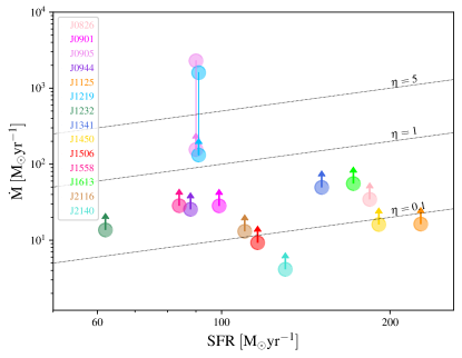
As described above, deriving accurate estimates requires precise knowledge of the physical conditions in the outflowing gas, the properties of the interstellar medium where the outflow propagates, and the outflow geometry and kinematics. We discussed above the assumptions adopted here to determine these first-order estimates, and we discussed how they represent lower limits on the actual outflow rates for most of the galaxies in our sample. We stress that the biggest uncertainty in calculating the mass outflow rates is introduced by the uncertainties on the (H) estimates. In our study, the leading uncertainty on (H) arises from the difficulty of breaking the degeneracy between and for saturated Mg II doublet lines, when additional constraints from the Fe II multiplet are not available. We also report in Table 5 the mass loading factor, /SFR. compares the amount of gas entrained by the outflow to the amount of gas actively being converted into stars, and it represents a useful way to quantify how the outflow may impact the future evolution of the host galaxy, as it relates to the rate at which gas is being removed from the galaxy to the rate at which it is currently creating stars.
| ID | 11Mass outflow rate calculated using Equation 7 and the blueshifted hydrogen column density reported in Table 2, column 6. | 22Mass outflow rate calculated using Equation 7 and the highest value between column 6 and 7 of Table 2 (only blueshifted components). | 33Mass loading factor, i.e. , calculated using as . | 44Mass loading factor calculated using as and applying a factor of 12 correction to the upper limit values. |
|---|---|---|---|---|
| [] | [] | |||
| J0826 | 34 | 85 | 0.46 | 5.52 |
| J0901 | 28 | 49 | 0.49 | 5.93 |
| J0905 | 156 | 2288∗ | 25.43 | 25.43 |
| J0944 | 25 | 80 | 0.91 | 10.94 |
| J1125 | 16 | 97 | 0.43 | 5.10 |
| J1219 | 132 | 1598∗ | 17.56 | 17.56 |
| J1232 | 14 | 26 | 0.42 | 5.04 |
| J1341 | 49 | 162 | 1.08 | 12.91 |
| J1450 | 16 | 25 | 0.13 | 1.54 |
| J1506 | 9 | 25 | 0.22 | 2.63 |
| J1558 | 28 | 85 | 1.01 | 12.11 |
| J1613 | 55 | 0.32 | 3.87 | |
| J2116 | 13 | 0.12 | 1.42 | |
| J2140 | 4 | 0.03 | 0.38 |
Figure 14 shows the mass outflow rates as calculated using Mg II only constraints (Table 5, column 1) as a function of the star formation rate. As discussed these are lower limits on the total ionized gas mass outflow rates. In order to demonstrate the potential magnitude of the systematic underestimate of derived using Mg II only, we show the values calculated using bounds on from Fe II fits (Table 5, column 2) for the two sources (J0905 and J1219) in our sample that have the most robust estimates on and which are therefore not lower limits. The two estimates for J0905 and J1219 are connected by lines, to facilitate comparison. There is a large correction for these two sources between the Mg II only estimates (lower limits) and the more robust estimates (not lower limits), of factors of 15 and 12, respectively. The rest of the galaxies in the sample might have a similar magnitude correction if better constraints on (H) from the Fe II absorption lines were available. Applying similar corrections to the rest of the sample (i.e. to the values reported in Table 5) as those obtained for J0905 and J1219, we would infer mass outflow rates in the range for our galaxies.
Figure 14 also includes lines of constant mass loading factors, . The two galaxies with more robust constraints on , J0905 and J1219, exhibit values of the order of 25 and 17, respectively. Such high values of the mass loading factor indicate that the outflows are ejecting gas at a much higher rate than the production rate of stars. Similar values are found in ultraluminous infrared galaxies (ULIRGs) at (Rupke et al., 2005c). While the mass outflow rates are first-order estimates only, they are informative to verify that the observed starburst-driven outflows can clearly affect the evolution of their host galaxies by actively removing substantial amounts of gas. The mass outflow rates for J0905 and J1219 are estimated to be 2200 and 1500 , which are exceptionally high mass outflow rates. This finding is consistent with results based on observations of molecular gas for two galaxies (J0905 and J1341) in our sample (Geach et al., 2014, 2018). In particular, Geach et al. (2014) use the IRAM Plateau de Bure interferometer to study the CO(2-1) emission line, a tracer of the bulk of the cold molecular gas reservoir, in the galaxy J0905. They find that a third of the total molecular gas content appears to have been ejected on a scale of approximately 10 kpc. They estimate that the kinetic energy associated with the outflowing component is consistent with the momentum flux available from stellar radiation pressure, demonstrating that nuclear starbursts are capable of ejecting large amounts of cold gas from the central regions of galaxies.
As discussed in Section 4.3.4, the cold gas outflow phase is most likely produced by a combination of multiple physical processes. Therefore the high mass loading factors derived here do not necessarily refer to a single production mechanism of the cool gas. However, as a reference, we compare our estimates with predictions from Lochhaas et al. (2021), who model hot supersonic winds driven by supernovae energy injection in star-forming galaxies. The authors derive the characteristic momentum rates of hot galactic winds that can undergo single-phase cooling on large scales and produce cold gas as a function of the SFR of the galaxy. Interestingly, the predicted velocities of the wind at the maximum wind momentum rate for SFRs similar to our galaxies are compatible with the highest velocity absorption components in our spectra. However, most of our sample shows higher mass loading factors than the theoretical maximum predicted by their model. This would imply that our observations do not trace only cool outflows that obtained their momentum directly from the free-flowing hot wind, but rather that there may be some mass loading outside the wind-driving region. This supports the hypothesis that the cold gas outflow phase may have multiple origins.
In summary, when robust constraints from the Fe II multiplet are available we find extreme mass outflow rates () and values of . If similar corrections are applied to the rest of the galaxies, they would have in the range and 90% of the sample would have .
5 Summary and Conclusions
We use new optical Keck/HIRES spectroscopy of 14 compact starburst galaxies at z 0.5 to probe the small-scale structure of the powerful galactic outflows observed in our sample, gain insights into the role of various physical mechanisms in these extreme feedback episodes, and investigate their potential impact on the evolution of their host galaxies. These galaxies are massive (10), extremely compact (half-light radius few hundred pc), have very high star formation rates (mean ) and star formation surface densities (mean ), and host extremely fast (mean maximum velocity ) outflows traced by Mg II absorption lines (Tremonti et al., 2007; Davis et al., (submitted). The high resolution ( 8 ) spectra presented here cover a suite of Mg and Fe absorption lines (Mg II2796, 2803 doublet, Mg I2852, and Fe II2344, 2374, 2582, 2587, 2600 multiplet). This exquisite data set allows us to directly measure precise column densities and covering fractions () as a function of velocity for these ions and characterize the kinematics of the cool gas outflow phase (T 104 K). Our main conclusions are as follows:
1) Mg II absorption troughs best delineate the outflow kinematics among the ions studied here. We find a substantial variation in the absorption profiles in our data (Section 4.1 and Figure 8). In particular, there is a large variation in the minimum number of velocity components required to fit each profile, ranging from two to ten; in their widths, Doppler parameter , ranging from 8 to 344 with a mean of 106 ; and in their , with four galaxies having = 1, while the rest of the sample has as low as 0.12 and a mean value of 0.57.
2) We investigate if the multiple velocity components observed in our sample are related to the extreme and “bursty” star formation episodes in these galaxies. There is not a simple correlation between the number of bursts in the star formation history (SFH) and the Mg II absorption profiles (Section 4.1 and Figure 9). Galaxies showing similar Mg II absorption troughs can have a variety of SFHs and vice-versa.
3) Mg II emission is detected in 9/14 of the galaxies in our sample with velocity shifts of 0 to 450 from zsys. Emission filling is not an issue for most of our galaxies, which have highly blueshifted Mg II absorption lines (Section 4.2 and Figure 8). Indeed, 11/14 galaxies have less than four percent of the EW(Mg II) within 200 of zsys, where emission line filling can be important. We also find a lack of substantial Mg II absorption at the systemic velocity, and we present three possible explanations for this: the bulk of the interstellar medium (ISM) is expelled by the powerful outflows, biased observational selection criteria, and/or Mg II traces a cold gas phase formed “in-situ” within a galactic wind via thermal instabilities and condensation of the fast-moving hot phase.
4) Mg II, Mg I, and Fe II exhibit remarkably similar absorption profiles, suggesting these species reside in the same, low-ionization gas structures. However, Mg II has on average a higher at a given outflow velocity than Fe II, and in all cases a higher than neutral Mg, implying that the absorbing clouds are not homogeneous (Section 4.3.2). This result is in agreement with theoretical predictions that the coolest and densest gas is typically located in the more internal and self-shielded part of the clouds.
5) We find that does not display a unique trend with velocity (Section 4.3.3 and Figure 10). This variation, along with the variation of the absorption profiles, may capture the complex morphology of kpc scale, inhomogeneously-distributed, clumpy gas, and the intricacy of the material in the turbulent mixing layers between the cold and the hot phases. Moreover, other observations of our galaxies are consistent with models in which the outflows decelerate with time as they expand into the CGM.
6) We consider the possibility of Fe II as the primary tracer of the entrained cool gas phase component and Mg II as the tracer of the cooled hot wind material and examine how their ratio varies as a function of outflow velocity. Several of the galaxies in our sample do not have Fe II detected at the highest outflow velocities, indicating a lower mixing fraction of entrained cool gas. This suggests that the cold gas at the highest velocities in these galaxies most likely directly condensed out of the hot wind phase, as suggested by some theoretical models (Section 4.3.4, Figure 11 and 12).
7) We estimate mass outflow rates for the observed winds in our sample and discuss how these estimates are lower limits on the actual outflow rates for most of the galaxies (Section 4.5 and Figure 14). We show that the two galaxies in our sample that have robust constraints from the Fe II multiplet have extremely high mass outflow rates () and mass loading factors (1725). If similar corrections are applied to the rest of the galaxies we infer 502200 with a typical value of 5. This demonstrates that starburst galaxies are capable of ejecting very large amounts of cold gas which will substantially impact their future evolution.
The galaxy sample studied here provides a prime opportunity to investigate star formation and feedback at its most extreme. In a forthcoming paper based on integral field unit Keck/KCWI spectra, we will focus on studying the morphology, physical extent, and kinematics of the outflows in our sample. Such data on these galaxies provides strong observational constraints to theoretical simulations that aim to implement realistic stellar-driven galactic outflows. The comparison of outflow properties between simulations and observations will advance our understanding of galactic feedback, especially from stellar processes, during a critical stage of massive galaxy evolution.
Acknowledgements
We thank the referee for her/his time to provide a constructive report. The referee’s thoughtful comments have helped to improve the clarity of the manuscript. We acknowledge support from the National Science Foundation (NSF) under a collaborative grant (AST-1813299, 1813365, 1814233, 1813702, and 1814159) and from the Heising-Simons Foundation grant 2019-1659. S. P. and A. L. C. acknowledge support from the Ingrid and Joseph W. Hibben endowed chair at UC San Diego. The data presented herein were obtained at the W. M. Keck Observatory, which is operated as a scientific partnership among the California Institute of Technology, the University of California, and the National Aeronautics and Space Administration. The Observatory was made possible by the generous financial support of the W. M. Keck Foundation. The authors wish to recognize and acknowledge the very significant cultural role and reverence that the summit of Maunakea has always had within the indigenous Hawaiian community. We are most fortunate to have the opportunity to conduct observations from this mountain.
Appendix A Notes and Fits of Individual Targets
Figures 1524 show the normalized spectra of the other 10 galaxies in our sample centered on the transitions relevant to this study: Mg II2796,2803Å, Mg I2803Å, Fe II2382Å, Fe II2600Å, Fe II2344Å, Fe II2586Å, and Fe II2374Å. For each galaxy, we show the Mg I2853 best fit profile as derived following the constrained approach. Details for each galaxy are given below.
J0826+4305
Figure 15 shows our best fit to the Mg II, Mg I, and Fe II absorption lines in the galaxy J0826+4305 (hereafter J0826). J0826 spectrum shows Mg II emission within and of zsys. In this galaxy, we see strong absorption from Mg II falling within and of zsys. The Mg II trough is well described by eight velocity components that show complex kinematics. The Mg II2796 and Mg II2803 troughs exhibit comparable intensity at all velocities for seven over eight components. In that case, the Mg II traces optically thick gas. As the lines are not black the covering fraction () determines the shape of the absorption troughs. The most blueshifted component ( ) has 1 and = 1. In this galaxy, we note that the increases with increasing blueshift from zsys. We detect Fe II and Mg I absorption within and of zsys, which we model using two velocity components. They have quite good kinematic correspondence (within the errors) to two Mg II components. However, the Fe II and Mg I (independent) fit find the least blueshifted component to be substantially broader than the corresponding Mg II (20 and 55%, respectively). We find both Fe II components to trace optically thin gas and have lower than Mg II (32 and 45% of (Mg II), respectively). Based on comparison of (Mg II)meas and (Mg II)inf, we conclude that the Mg II fit gives a lower limit estimate of the N(Mg II) for the two components we have detection of both Mg II and Fe II. The actual (Mg II) is 3 times larger than the measured one. As for previous targets we favor the Mg I constrained fit solution because the neutral Mg fraction must be less than one percent to produce an optically thin Mg I2853 trough with =1 as found by the independent fit. The constrained fit finds for both Mg I components a smaller than Mg II (28 and 33% of (Mg II), respectively).
J0901+0314
Figure 16 shows our best fit to the Mg II, Mg I, and Fe II absorption lines in the galaxy J0901+0314 (hereafter J0901). J0901 spectrum exhibits Mg II redshifted emission ( ) within and of zsys. In this galaxy, we detect strong absorption from Mg II falling within and of zsys. The Mg II trough is well characterized by four velocity components that exhibit complex kinematics. One Mg II2796 component blends together with three Mg II2803 ones. Our Mg II best fit includes one optically thin component (at ) with =1, and three more blueshifted components. The latters trace optically thick gas, with Mg II2796 and Mg II2803 showing nearly identical intensity at all velocities. Their absorption profiles are not black and their shape is determined by . We detect Fe II and Mg I absorption within and of zsys, which we model using two velocity components. We find that one of these two components has a good kinematics correspondence (comparable and to within the error bars) to one Mg II component. for both Fe II and Mg I (from the constrained fit), is found to be lower than (Mg II), 52% and 43% of (Mg II), respectively. The values of (Mg II)meas and (Mg II)inf for the component detected at represent a lower limit (the actual (Mg II) is 3 times larger), while agreeing well within the errors for the component detected at . The independent Mg I fit shows kinematics in line with the constrained fit. However, to be a valid solution, the neutral Mg fraction must be less than one percent. The second and more blueshifted Fe II and Mg I (from the independent fit) component in our model show a substantially broader absorption profile (46% and 72% of (Mg II), respectively). Based on comparison of (Mg II)meas and (Mg II)inf we infer that Mg II should be optically thin, but that is inconsistent with the nearly identical intensity of Mg II2796 and Mg II2803. We attribute this discrepancy to the low SNR in the Fe II and Mg I profiles blueward of that is inadequate to definitively constrain the kinematics of the absorption troughs.
J0944+0930
Figure 17 shows our best fit to the Mg II, Mg I, and Fe II absorption lines in the galaxy J0944+0930 (hereafter J0944). J0944 spectrum does not show Mg II emission. In this galaxy, we see strong absorption from Mg II falling within and of zsys. The Mg II trough is well described by five velocity components that show convoluted kinematics. Most of them (four Mg II2796, and four Mg II2803) blend together. We find that the profile shape for all Mg II components is determined by the optical depth, rather than the , that is unity. Our Mg II best fit includes only one optically thick component (at ), the remaining components trace optically thin gas. The Mg I trough has a remarkable alignment with Mg II. We model the Mg I absorption using five components, as well. In the constrained fit the five Mg I components are described by lower compared to Mg II, with values in the range of of (Mg II). The independent Mg I fit finds a great agreement in terms of kinematics with the corresponding Mg II components. However, to be a valid solution, the neutral Mg fraction must be less than one percent. Therefore, we favor the constrained fit result. We detect Fe II within and of zsys, that we model using three velocity components. They have good alignment with three Mg II components, but they are characterized by broader line profiles (in the range of 30 to 50 %). Based on a comparison of (Mg II)meas and (Mg II)inf we conclude that the Mg II fit provides a decent estimate of the N(Mg II). However, we note that the difference in the kinematics of the two absorption troughs makes the comparison of the not accurate.
J11250145
Figure 18 shows our best fit to the Mg II, Mg I, and Fe II absorption lines in the galaxy J11250145 (hereafter J1125). J1125 spectrum does not exhibit Mg II emission. In this galaxy, we see absorption from Mg II falling within and of zsys. The Mg II trough is well described by two optically thick velocity components. The identical intensity at all velocities of the Mg II absorption lines indicates that their profile shapes are determined by . We detect Mg I and Fe II within the same velocity range as Mg II. We model the Mg I and Fe II troughs using two components and find a remarkable kinematic correspondence (comparable and to within the errors) to the Mg II fit. Both, Mg I (from constrained fit) and Fe II absorption profiles are described well by lower than Mg II(50 and 43 % of (Mg II), respectively). Comparing (Mg II)meas and (Mg II)inf we argue that the Mg II fit provides a lower limit estimate of the N(Mg II) and that the actual central optical depth for the two Mg II2803 components is closer to 9, 22 (rather than 2 and 3 as measured from the Mg II fit).
J1219+0336
Figure 19 shows our best fit to the Mg II, Mg I, and Fe II absorption lines in the galaxy J1219+0336 (hereafter J1219). J1219 spectrum very clearly shows Mg II2803 emission within and of zsys. The corresponding Mg II2796 line is not obvious because of Mg II2803 absorption at the same wavelengths. The inclusion of an emission component in the model improves the overall fit to the Mg II absorption trough. In this galaxy, we see strong absorption from Mg II falling within and of zsys. The Mg II trough is well described by four velocity components that blend together producing extremely intricate kinematics. Our Mg II best fit includes one optically thin component (at ) with =1. The remaining three components trace optically thick gas, and their profiles are shaped by . We detect Mg I within and of zsys. We model the Mg I trough using three components that show a good qualitative alignment with Mg II. The constrained Mg I fit finds lower than Mg II, in the range % of (Mg II). In our independent Mg I fit model, we find for the most blueshifted component an excellent kinematic agreement to the corresponding Mg II one ( and within the errors). The other two components show kinematics substantially different from Mg II. We attribute this difference to the low SNR in the Mg I profile redward of which is not sufficient to conclusively constrain the kinematics of the absorption troughs. We detect Fe II within and of zsys. Before performing the Fe II fit, we identify and model the Mn II 2576, 2594, and 2606 triplet (yellow solid lines). We model the Mg I trough using three components that show extremely good kinematic agreement with Mg II. We find Fe II to have lower than Mg II (53, 46, and 55 % of (Mg II), respectively). Based on a comparison of (Mg II)meas and (Mg II)inf, we conclude that the Mg II fit gives only a lower limit to the N(Mg II), and that the actual for the two Mg II2803 components, is closer to 90, 21, and 91 (than 10, 1.2, and 10).
J1506+5402
Figure 19 shows our best fit to the Mg II, Mg I, and Fe II absorption lines in the galaxy J1506+5402 (hereafter J1506). J1506 spectrum very clearly shows redshifted (126 ) Mg II2803 emission from to of zsys. The corresponding Mg II2796 line is not obvious because of Mg II2803 absorption at the same wavelengths. The inclusion of an emission component in the model improves the overall fit to the Mg II absorption trough. In this galaxy, we see strong absorption from Mg II falling within and of zsys. The Mg II trough is well characterized by five velocity components that blend together creating complex kinematics. We find that all Mg II components trace optically thin gas, and their absorption profiles are shaped by the optical depth, rather than the , that is unity. We detect Mg I within and of zsys. We model the Mg I trough using two components that show a good alignment with Mg II. The constrained fit finds lower (Mg I) than Mg II (45 and 60% of (Mg II), respectively). Adopting the independent Mg I fit we find the two Mg I components to be slightly narrower (7 and 20%) than the corresponding Mg II. In both cases, the Mg I traces optically thin gas as Mg II. However, we favor the constrained fit solution since to have (Mg I) = 1 the neutral Mg fraction must be less than one percent. We detect Fe II within and of zsys. We model the Fe II troughs using two components that show a good alignment with Mg II. However, we note that (Fe II) is 38% narrower than (Mg II) for the most blueshifted component, and 15% broader for the other one. Despite the discrepancy between their kinematics, we find a very good agreement between (Mg II)meas and (Mg II)infwithin the errors.
J1558+3957
Figure 19 shows our best fit to the Mg II, Mg I, and Fe II absorption lines in the galaxy J1558+3957 (hereafter J1558). J1558 spectrum distinctly shows slightly redshifted (57 ) Mg II2803 emission within and of zsys. The corresponding Mg II2796 line is not apparent because of Mg II2803 absorption at the same wavelengths. The inclusion of an emission component in the model improves the fit to the Mg II absorption trough. In this galaxy, we see strong absorption from Mg II falling within and of zsys. The Mg II trough is well described by four velocity components that exhibit intricate kinematics. Our Mg II best fit finds the most blueshifted component to be optically thing and with = 1. For the other three components, the measured equivalent width ratio for Mg II2796 and Mg II2803 is not consistent (30 to 65% lower) with the optically thin limit. They trace optically thick gas and their absorption profiles are shaped by 1. We detect weak Mg I within and of zsys. We model the Mg I trough using two components. The constrained fit finds Mg I to be characterized by lower than Mg II (31 and 50% of (Mg II), respectively). The independent Mg I fit finds two components that show a good qualitative alignment with Mg II, but fairly broader absorption profiles (56 and 18% respectively). We prefer the constrained fit solution since to have optically thin Mg I for the least blueshifted component and (Mg I) = 1 the neutral Mg fraction must be less than one percent. We detect Fe II within and of zsys. We model Fe II using only one component with a good kinematic correspondence to one Mg II component. We find that Fe II traces optically thin gas and the profile is well described by a lower than Mg II(51 % of (Mg II)). Based on comparison of (Mg II)meas and (Mg II)inf, we conclude that the Mg II fit gives a lower limit estimate of the N(Mg II) for the component we have detection of both Mg II and Fe II. The actual (Mg II) is 4 times larger than the measured one.
J1613+2834
Figure 19 shows our best fit to the Mg II, Mg I, and Fe II absorption lines in the galaxy J1613+2834 (hereafter J1613). J1613 spectrum clearly exhibits redshifted (284 ) Mg II2803 emission within and of zsys. The corresponding Mg II2796 line is not obvious because of Mg II2803 absorption at the same wavelengths. The inclusion of an emission component in the model improves the fit to the Mg II absorption trough. In this galaxy, we see strong absorption from Mg II falling within and of zsys. The Mg II trough is well described by five velocity components that blend together and produce complicated kinematics. We find that Mg II traces optically thick gas. The measured equivalent width ratio for Mg II2796 and Mg II2803 is not consistent (25 to 45% lower) with the optically thin limit. The absorption profile of all five components is well described by 1. We do not identify any significant absorption trough in the Mg I spectral region. We detect weak Fe II in correspondence with the most blueshifted Mg II component. We model the Fe II trough using only one component. Despite the Fe II component showing a good alignment with Mg II (similar within the errors), our best fit finds a significantly (44%) broader absorption profile. We attribute this to the low SNR in the Fe II spectral region. According to our best fit Fe II traces optically thin gas. We infer from the Fe II fit that the corresponding Mg II component should be less optically thick, with (Mg II)inf= 2.7 and (Mg II)meas= 10. This is probably due to a difference in the kinematics ((Mg II) = 57% (Fe II)) of the two absorption lines that makes the comparison of the not accurate, underestimating (Mg II)inf.
J21160624
Figure 23 shows our best fit to the Mg II, Mg I, and Fe II absorption lines in the galaxy J21160624 (hereafter J2116). J2116 spectrum does not exhibit Mg II emission. In this galaxy, we identify two Mg II absorption troughs at around and of zsys, respectively. We find that the most blueshifted Mg II component ( ) traces optically thick gas and its profile shape is characterized by 1. The least blueshifted Mg II component ( ) is close to the transition between optically thin and thick gas, with =0.97. The measured equivalent width ratio for Mg II2796 and Mg II2803 is 25% lower than the theoretical value. Therefore, we conclude that the absorption profile shape is determined by the 1 rather than the optical depth. We detect weak Mg I and Fe II in correspondence with the least blueshifted Mg II component. We model Mg I and Fe II using only one component. The independent Mg I fit finds a substantially broader (60%) absorption profile than the corresponding Mg II. We attribute this discrepancy to the difficulties of identifying such a weak absorption trough. As for previous targets we favor the Mg I constrained fit solution because the neutral Mg fraction must be less than one percent to produce an optically thin Mg I2853 trough with =1 as found by the independent fit. The constrained fit finds Mg I to be characterized by a smaller than Mg II (32% of (Mg II)). The Fe II fit shows a very good kinematic agreement with Mg II (similar and within the errors). The Fe II absorption traces optically thin gas with =1. We find a good agreement between (Mg II)meas and (Mg II)infwithin the errors.
J2140+1209
Figure 24 shows our best fit to the Mg II, Mg I, and Fe II absorption lines in the galaxy J2140+1209 (hereafter J2140). J2140 spectrum does not exhibit Mg II emission. In this galaxy, we identify strong Mg II absorption troughs falling within and of zsys. The Mg II trough is well described by five velocity components that marginally blend together (one Mg II2796 and three Mg II2803 components). We find that Mg II traces optically thick gas for the least blueshifted component ( ). The measured equivalent width ratio for Mg II2796 and Mg II2803 is not consistent (40% lower) with the optically thin limit. The absorption profile of this component is shaped by 1. The remaining four components trace optically thin gas and their profile shape is well described by the optical depth. We do not identify any significant absorption trough in the Mg I and Fe II spectral regions.

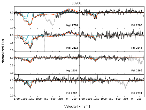
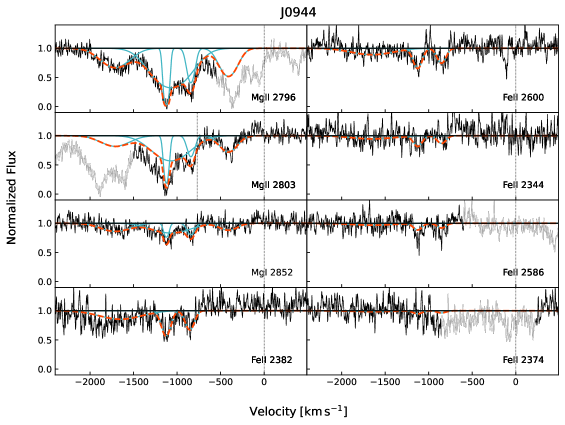
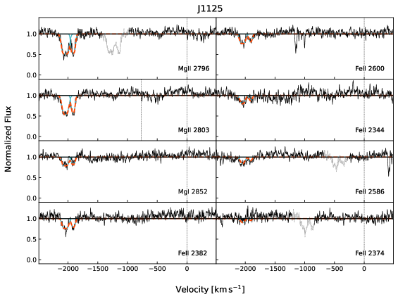
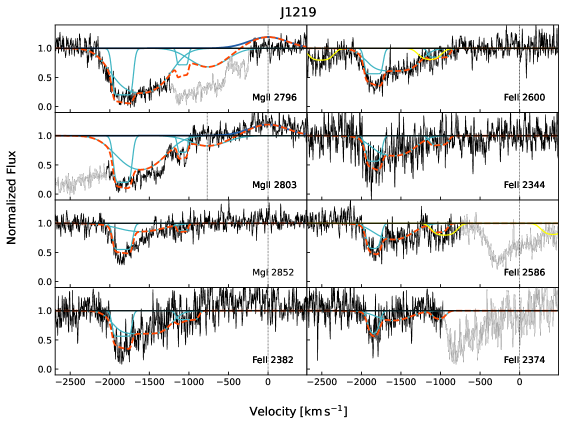
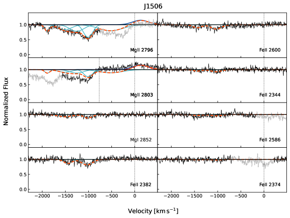
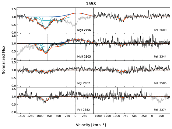
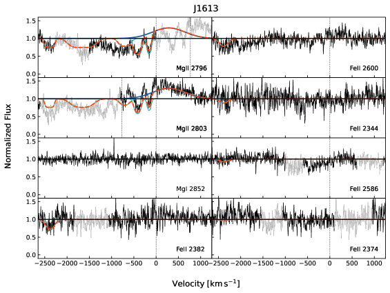
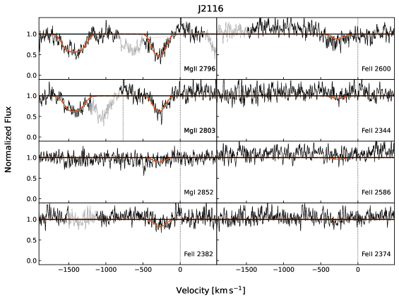
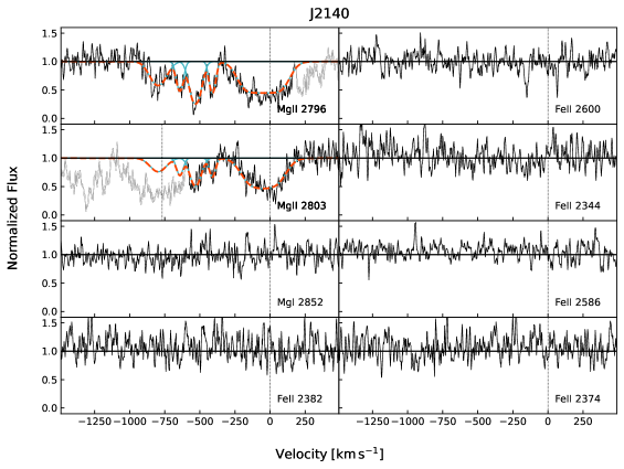
References
- Aihara et al. (2011) Aihara, H., Allende Prieto, C., An, D., et al. 2011, ApJS, 193, 29, doi: 10.1088/0067-0049/193/2/29
- Arav et al. (1999) Arav, N., Korista, K. T., de Kool, M., Junkkarinen, V. T., & Begelman, M. C. 1999, ApJ, 516, 27, doi: 10.1086/307073
- Armillotta et al. (2016) Armillotta, L., Fraternali, F., & Marinacci, F. 2016, MNRAS, 462, 4157, doi: 10.1093/mnras/stw1930
- Asplund et al. (2021) Asplund, M., Amarsi, A. M., & Grevesse, N. 2021, A&A, 653, A141, doi: 10.1051/0004-6361/202140445
- Bolatto et al. (2013) Bolatto, A. D., Wolfire, M., & Leroy, A. K. 2013, ARA&A, 51, 207, doi: 10.1146/annurev-astro-082812-140944
- Bordoloi et al. (2014) Bordoloi, R., Lilly, S. J., Hardmeier, E., et al. 2014, ApJ, 794, 130, doi: 10.1088/0004-637X/794/2/130
- Brüggen & Scannapieco (2016) Brüggen, M., & Scannapieco, E. 2016, ApJ, 822, 31, doi: 10.3847/0004-637X/822/1/31
- Burchett et al. (2021) Burchett, J. N., Rubin, K. H. R., Prochaska, J. X., et al. 2021, ApJ, 909, 151, doi: 10.3847/1538-4357/abd4e0
- Bustard et al. (2016) Bustard, C., Zweibel, E. G., & D’Onghia, E. 2016, ApJ, 819, 29, doi: 10.3847/0004-637X/819/1/29
- Cappellari (2017) Cappellari, M. 2017, MNRAS, 466, 798, doi: 10.1093/mnras/stw3020
- Cappellari & Emsellem (2004) Cappellari, M., & Emsellem, E. 2004, PASP, 116, 138, doi: 10.1086/381875
- Chisholm et al. (2020) Chisholm, J., Prochaska, J. X., Schaerer, D., Gazagnes, S., & Henry, A. 2020, MNRAS, 498, 2554, doi: 10.1093/mnras/staa2470
- Chisholm et al. (2016) Chisholm, J., Tremonti Christy, A., Leitherer, C., & Chen, Y. 2016, MNRAS, 463, 541, doi: 10.1093/mnras/stw1951
- Choi et al. (2016) Choi, J., Dotter, A., Conroy, C., et al. 2016, ApJ, 823, 102, doi: 10.3847/0004-637X/823/2/102
- Churchill et al. (2003) Churchill, C. W., Vogt, S. S., & Charlton, J. C. 2003, AJ, 125, 98, doi: 10.1086/345513
- Conroy & Gunn (2010) Conroy, C., & Gunn, J. E. 2010, ApJ, 712, 833, doi: 10.1088/0004-637X/712/2/833
- Conroy et al. (2009) Conroy, C., Gunn, J. E., & White, M. 2009, ApJ, 699, 486, doi: 10.1088/0004-637X/699/1/486
- Cooper et al. (2009) Cooper, J. L., Bicknell, G. V., Sutherland, R. S., & Bland-Hawthorn, J. 2009, ApJ, 703, 330, doi: 10.1088/0004-637X/703/1/330
- Davies et al. (2019) Davies, R. L., Förster Schreiber, N. M., Übler, H., et al. 2019, ApJ, 873, 122, doi: 10.3847/1538-4357/ab06f1
- Davis et al. (2014) Davis, T. A., Young, L. M., Crocker, A. F., et al. 2014, MNRAS, 444, 3427, doi: 10.1093/mnras/stu570
- DeFelippis et al. (2021) DeFelippis, D., Bouché, N. F., Genel, S., et al. 2021, ApJ, 923, 56, doi: 10.3847/1538-4357/ac2cbf
- Diamond-Stanic et al. (2012) Diamond-Stanic, A. M., Moustakas, J., Tremonti, C. A., et al. 2012, ApJ, 755, L26, doi: 10.1088/2041-8205/755/2/L26
- Diamond-Stanic et al. (2021) Diamond-Stanic, A. M., Moustakas, J., Sell, P. H., et al. 2021, arXiv e-prints, arXiv:2102.11287. https://arxiv.org/abs/2102.11287
- Efstathiou et al. (2000) Efstathiou, A., Rowan-Robinson, M., & Siebenmorgen, R. 2000, MNRAS, 313, 734, doi: 10.1046/j.1365-8711.2000.03269.x
- Eldridge & Stanway (2016) Eldridge, J. J., & Stanway, E. R. 2016, MNRAS, 462, 3302, doi: 10.1093/mnras/stw1772
- Erb et al. (2012) Erb, D. K., Quider, A. M., Henry, A. L., & Martin, C. L. 2012, ApJ, 759, 26, doi: 10.1088/0004-637X/759/1/26
- Everett et al. (2008) Everett, J. E., Zweibel, E. G., Benjamin, R. A., et al. 2008, ApJ, 674, 258, doi: 10.1086/524766
- Fielding & Bryan (2022) Fielding, D. B., & Bryan, G. L. 2022, ApJ, 924, 82, doi: 10.3847/1538-4357/ac2f41
- Fielding et al. (2020) Fielding, D. B., Ostriker, E. C., Bryan, G. L., & Jermyn, A. S. 2020, ApJ, 894, L24, doi: 10.3847/2041-8213/ab8d2c
- Geach et al. (2013) Geach, J. E., Hickox, R. C., Diamond-Stanic, A. M., et al. 2013, ApJ, 767, L17, doi: 10.1088/2041-8205/767/1/L17
- Geach et al. (2014) —. 2014, Nature, 516, 68, doi: 10.1038/nature14012
- Geach et al. (2018) Geach, J. E., Tremonti, C., Diamond-Stanic, A. M., et al. 2018, ArXiv e-prints, arXiv:1807.09789. https://arxiv.org/abs/1807.09789
- Gritton et al. (2017) Gritton, J. A., Shelton, R. L., & Galyardt, J. E. 2017, ApJ, 842, 102, doi: 10.3847/1538-4357/aa756d
- Gronke & Oh (2018) Gronke, M., & Oh, S. P. 2018, MNRAS, 480, L111, doi: 10.1093/mnrasl/sly131
- Gronke & Oh (2020) —. 2020, MNRAS, 492, 1970, doi: 10.1093/mnras/stz3332
- Häußler et al. (2013) Häußler, B., Bamford, S. P., Vika, M., et al. 2013, MNRAS, 430, 330, doi: 10.1093/mnras/sts633
- Heckman et al. (2015) Heckman, T. M., Alexandroff, R. M., Borthakur, S., Overzier, R., & Leitherer, C. 2015, ApJ, 809, 147, doi: 10.1088/0004-637X/809/2/147
- Heckman & Borthakur (2016) Heckman, T. M., & Borthakur, S. 2016, ApJ, 822, 9, doi: 10.3847/0004-637X/822/1/9
- Heckman et al. (2000) Heckman, T. M., Lehnert, M. D., Strickland, D. K., & Armus, L. 2000, ApJS, 129, 493, doi: 10.1086/313421
- Hopkins et al. (2014) Hopkins, P. F., Kereš, D., Oñorbe, J., et al. 2014, MNRAS, 445, 581, doi: 10.1093/mnras/stu1738
- Hopkins et al. (2012) Hopkins, P. F., Quataert, E., & Murray, N. 2012, MNRAS, 421, 3522, doi: 10.1111/j.1365-2966.2012.20593.x
- Jenkins (2009) Jenkins, E. B. 2009, ApJ, 700, 1299, doi: 10.1088/0004-637X/700/2/1299
- Johnson et al. (2021) Johnson, B. D., Leja, J., Conroy, C., & Speagle, J. S. 2021, ApJS, 254, 22, doi: 10.3847/1538-4365/abef67
- Jones et al. (2018) Jones, T., Stark, D. P., & Ellis, R. S. 2018, ApJ, 863, 191, doi: 10.3847/1538-4357/aad37f
- Kennicutt & Evans (2012) Kennicutt, R. C., & Evans, N. J. 2012, ARA&A, 50, 531, doi: 10.1146/annurev-astro-081811-125610
- Kereš et al. (2005) Kereš, D., Katz, N., Weinberg, D. H., & Davé, R. 2005, MNRAS, 363, 2, doi: 10.1111/j.1365-2966.2005.09451.x
- Kormendy & Ho (2013) Kormendy, J., & Ho, L. C. 2013, ARA&A, 51, 511, doi: 10.1146/annurev-astro-082708-101811
- Kornei et al. (2012) Kornei, K. A., Shapley, A. E., Martin, C. L., et al. 2012, ApJ, 758, 135, doi: 10.1088/0004-637X/758/2/135
- Kroupa (2001) Kroupa, P. 2001, MNRAS, 322, 231, doi: 10.1046/j.1365-8711.2001.04022.x
- Krumholz & Thompson (2013) Krumholz, M. R., & Thompson, T. A. 2013, MNRAS, 434, 2329, doi: 10.1093/mnras/stt1174
- Lehnert & Heckman (1996) Lehnert, M. D., & Heckman, T. M. 1996, ApJ, 472, 546, doi: 10.1086/178086
- Leja et al. (2019) Leja, J., Carnall, A. C., Johnson, B. D., Conroy, C., & Speagle, J. S. 2019, ApJ, 876, 3, doi: 10.3847/1538-4357/ab133c
- Lochhaas et al. (2018) Lochhaas, C., Thompson, T. A., Quataert, E., & Weinberg, D. H. 2018, MNRAS, 481, 1873, doi: 10.1093/mnras/sty2421
- Lochhaas et al. (2021) Lochhaas, C., Thompson, T. A., & Schneider, E. E. 2021, MNRAS, 504, 3412, doi: 10.1093/mnras/stab1101
- Marigo et al. (2008) Marigo, P., Girardi, L., Bressan, A., et al. 2008, A&A, 482, 883, doi: 10.1051/0004-6361:20078467
- Martin (1998) Martin, C. L. 1998, ApJ, 506, 222, doi: 10.1086/306219
- Martin & Bouché (2009) Martin, C. L., & Bouché, N. 2009, ApJ, 703, 1394, doi: 10.1088/0004-637X/703/2/1394
- Martin et al. (2012) Martin, C. L., Shapley, A. E., Coil, A. L., et al. 2012, ApJ, 760, 127, doi: 10.1088/0004-637X/760/2/127
- McCourt et al. (2015) McCourt, M., O’Leary, R. M., Madigan, A.-M., & Quataert, E. 2015, MNRAS, 449, 2, doi: 10.1093/mnras/stv355
- McQuinn et al. (2019) McQuinn, K. B. W., van Zee, L., & Skillman, E. D. 2019, ApJ, 886, 74, doi: 10.3847/1538-4357/ab4c37
- Meurer et al. (1997) Meurer, G. R., Heckman, T. M., Lehnert, M. D., Leitherer, C., & Lowenthal, J. 1997, AJ, 114, 54, doi: 10.1086/118452
- Morton (1991) Morton, D. C. 1991, ApJS, 77, 119, doi: 10.1086/191601
- Morton (2003) —. 2003, ApJS, 149, 205, doi: 10.1086/377639
- Murray et al. (2007) Murray, N., Martin, C. L., Quataert, E., & Thompson, T. A. 2007, ApJ, 660, 211, doi: 10.1086/512660
- Murray et al. (2011) Murray, N., Ménard, B., & Thompson, T. A. 2011, ApJ, 735, 66, doi: 10.1088/0004-637X/735/1/66
- Murray et al. (2005) Murray, N., Quataert, E., & Thompson, T. A. 2005, ApJ, 618, 569, doi: 10.1086/426067
- Murray et al. (2010) —. 2010, ApJ, 709, 191, doi: 10.1088/0004-637X/709/1/191
- Nelson et al. (2021) Nelson, D., Byrohl, C., Peroux, C., Rubin, K. H. R., & Burchett, J. N. 2021, MNRAS, 507, 4445, doi: 10.1093/mnras/stab2177
- Nelson et al. (2019) Nelson, D., Pillepich, A., Springel, V., et al. 2019, MNRAS, 490, 3234, doi: 10.1093/mnras/stz2306
- O’Meara et al. (2015) O’Meara, J. M., Lehner, N., Howk, J. C., et al. 2015, AJ, 150, 111, doi: 10.1088/0004-6256/150/4/111
- Oppenheimer et al. (2010) Oppenheimer, B. D., Davé, R., Kereš, D., et al. 2010, MNRAS, 406, 2325, doi: 10.1111/j.1365-2966.2010.16872.x
- Peng et al. (2002) Peng, C. Y., Ho, L. C., Impey, C. D., & Rix, H.-W. 2002, AJ, 124, 266, doi: 10.1086/340952
- Peng et al. (2010) —. 2010, AJ, 139, 2097, doi: 10.1088/0004-6256/139/6/2097
- Perrotta et al. (2021) Perrotta, S., George, E. R., Coil, A. L., et al. 2021, ApJ, 923, 275, doi: 10.3847/1538-4357/ac2fa4
- Petter et al. (2020) Petter, G. C., Kepley, A. A., Hickox, R. C., et al. 2020, ApJ, 901, 138, doi: 10.3847/1538-4357/abb19d
- Prochaska et al. (2011) Prochaska, J. X., Kasen, D., & Rubin, K. 2011, ApJ, 734, 24, doi: 10.1088/0004-637X/734/1/24
- Prusinski et al. (2021) Prusinski, N. Z., Erb, D. K., & Martin, C. L. 2021, AJ, 161, 212, doi: 10.3847/1538-3881/abe85b
- Rubin et al. (2012) Rubin, K. H. R., Prochaska, J. X., Koo, D. C., & Phillips, A. C. 2012, ApJ, 747, L26, doi: 10.1088/2041-8205/747/2/L2610.48550/arXiv.1110.0837
- Rubin et al. (2014) Rubin, K. H. R., Prochaska, J. X., Koo, D. C., et al. 2014, ApJ, 794, 156, doi: 10.1088/0004-637X/794/2/156
- Rubin et al. (2011) Rubin, K. H. R., Prochaska, J. X., Ménard, B., et al. 2011, ApJ, 728, 55, doi: 10.1088/0004-637X/728/1/55
- Rubin et al. (2010) Rubin, K. H. R., Weiner, B. J., Koo, D. C., et al. 2010, ApJ, 719, 1503, doi: 10.1088/0004-637X/719/2/1503
- Rupke et al. (2005a) Rupke, D. S., Veilleux, S., & Sanders, D. B. 2005a, ApJS, 160, 87, doi: 10.1086/432886
- Rupke et al. (2005b) —. 2005b, ApJS, 160, 115, doi: 10.1086/432889
- Rupke et al. (2005c) —. 2005c, ApJ, 632, 751, doi: 10.1086/444451
- Rupke (2014) Rupke, D. S. N. 2014, IFSFIT: Spectral Fitting for Integral Field Spectrographs. http://ascl.net/1409.005
- Rupke et al. (2019) Rupke, D. S. N., Coil, A., Geach, J. E., et al. 2019, Nature, 574, 643, doi: 10.1038/s41586-019-1686-1
- Salim et al. (2018) Salim, S., Boquien, M., & Lee, J. C. 2018, ApJ, 859, 11, doi: 10.3847/1538-4357/aabf3c
- Salpeter (1955) Salpeter, E. E. 1955, ApJ, 121, 161, doi: 10.1086/145971
- Salvatier et al. (2016) Salvatier, J., Wiecki, T. V., & Fonnesbeck, C. 2016, PeerJ Computer Science, 2, e55
- Sato et al. (2009) Sato, T., Martin, C. L., Noeske, K. G., Koo, D. C., & Lotz, J. M. 2009, ApJ, 696, 214, doi: 10.1088/0004-637X/696/1/21410.48550/arXiv.0804.4312
- Savage & Sembach (1996) Savage, B. D., & Sembach, K. R. 1996, ARA&A, 34, 279, doi: 10.1146/annurev.astro.34.1.279
- Scannapieco & Brüggen (2015) Scannapieco, E., & Brüggen, M. 2015, ApJ, 805, 158, doi: 10.1088/0004-637X/805/2/158
- Schneider et al. (2020) Schneider, E. E., Ostriker, E. C., Robertson, B. E., & Thompson, T. A. 2020, ApJ, 895, 43, doi: 10.3847/1538-4357/ab8ae8
- Schneider & Robertson (2015) Schneider, E. E., & Robertson, B. E. 2015, ApJS, 217, 24, doi: 10.1088/0067-0049/217/2/24
- Schneider & Robertson (2017) —. 2017, ApJ, 834, 144, doi: 10.3847/1538-4357/834/2/144
- Sell et al. (2014) Sell, P. H., Tremonti, C. A., Hickox, R. C., et al. 2014, MNRAS, 441, 3417, doi: 10.1093/mnras/stu636
- Sheinis et al. (2002) Sheinis, A. I., Bolte, M., Epps, H. W., et al. 2002, PASP, 114, 851, doi: 10.1086/341706
- Silich et al. (2003) Silich, S., Tenorio-Tagle, G., & Muñoz-Tuñón, C. 2003, ApJ, 590, 791, doi: 10.1086/375133
- Silk & Rees (1998) Silk, J., & Rees, M. J. 1998, A&A, 331, L1. https://arxiv.org/abs/astro-ph/9801013
- Socrates et al. (2008) Socrates, A., Davis, S. W., & Ramirez-Ruiz, E. 2008, ApJ, 687, 202, doi: 10.1086/590046
- Somerville & Davé (2015) Somerville, R. S., & Davé, R. 2015, ARA&A, 53, 51, doi: 10.1146/annurev-astro-082812-140951
- Strauss et al. (2002) Strauss, M. A., Weinberg, D. H., Lupton, R. H., et al. 2002, AJ, 124, 1810, doi: 10.1086/342343
- Suzuki et al. (2005) Suzuki, N., Tytler, D., Kirkman, D., O’Meara, J. M., & Lubin, D. 2005, ApJ, 618, 592, doi: 10.1086/426062
- Thompson & Krumholz (2016) Thompson, T. A., & Krumholz, M. R. 2016, MNRAS, 455, 334, doi: 10.1093/mnras/stv2331
- Thompson et al. (2005) Thompson, T. A., Quataert, E., & Murray, N. 2005, ApJ, 630, 167, doi: 10.1086/431923
- Thompson et al. (2016) Thompson, T. A., Quataert, E., Zhang, D., & Weinberg, D. H. 2016, MNRAS, 455, 1830, doi: 10.1093/mnras/stv2428
- Tremonti et al. (2007) Tremonti, C. A., Moustakas, J., & Diamond-Stanic, A. M. 2007, ApJ, 663, L77, doi: 10.1086/520083
- Tumlinson et al. (2017) Tumlinson, J., Peeples, M. S., & Werk, J. K. 2017, ARA&A, 55, 389, doi: 10.1146/annurev-astro-091916-055240
- Uhlig et al. (2012) Uhlig, M., Pfrommer, C., Sharma, M., et al. 2012, MNRAS, 423, 2374, doi: 10.1111/j.1365-2966.2012.21045.x
- Veilleux et al. (2005) Veilleux, S., Cecil, G., & Bland-Hawthorn, J. 2005, ARA&A, 43, 769, doi: 10.1146/annurev.astro.43.072103.150610
- Veilleux et al. (2020) Veilleux, S., Maiolino, R., Bolatto, A. D., & Aalto, S. 2020, A&A Rev., 28, 2, doi: 10.1007/s00159-019-0121-9
- Vika et al. (2013) Vika, M., Bamford, S. P., Häußler, B., et al. 2013, MNRAS, 435, 623, doi: 10.1093/mnras/stt1320
- Vogt et al. (1994) Vogt, S. S., Allen, S. L., Bigelow, B. C., et al. 1994, in Society of Photo-Optical Instrumentation Engineers (SPIE) Conference Series, Vol. 2198, Instrumentation in Astronomy VIII, ed. D. L. Crawford & E. R. Craine, 362, doi: 10.1117/12.176725
- Weiner et al. (2009) Weiner, B. J., Coil, A. L., Prochaska, J. X., et al. 2009, ApJ, 692, 187, doi: 10.1088/0004-637X/692/1/187
- Whalen et al. (2022) Whalen, K. E., Hickox, R. C., Coil, A. L., et al. 2022, arXiv e-prints, arXiv:2209.13632. https://arxiv.org/abs/2209.13632
- Wright et al. (2010) Wright, E. L., Eisenhardt, P. R. M., Mainzer, A. K., et al. 2010, AJ, 140, 1868, doi: 10.1088/0004-6256/140/6/1868
- York et al. (2000) York, D. G., Adelman, J., Anderson, John E., J., et al. 2000, AJ, 120, 1579, doi: 10.1086/301513
- Zabl et al. (2021) Zabl, J., Bouché, N. F., Wisotzki, L., et al. 2021, MNRAS, 507, 4294, doi: 10.1093/mnras/stab2165
- Zhang & Thompson (2012) Zhang, D., & Thompson, T. A. 2012, MNRAS, 424, 1170, doi: 10.1111/j.1365-2966.2012.21291.x
- Zhang et al. (2017) Zhang, D., Thompson, T. A., Quataert, E., & Murray, N. 2017, MNRAS, 468, 4801, doi: 10.1093/mnras/stx822