Quasinormal Modes of Black holes in $f(Q)$ gravity

Abstract

In this work, we have studied the quasinormal modes of a black hole in a model of the type $f(Q)=\underset{n}{\sum}a_{n}\left(Q-Q_{0}\right)^{n}$ in $f(Q)$ gravity by using a recently introduced method known as Bernstein spectral method and confirmed the validity of the method with the help of well known Padé averaged higher order WKB approximation method. Here we have considered scalar perturbation and electromagnetic perturbation in the black hole spacetime and obtained the corresponding quasinormal modes. We see that for a non-vanishing nonmetricity scalar $Q_{0}$, quasinormal frequencies in scalar perturbation are greater than those in electromagnetic perturbation scenarios. On the other hand, the damping rate of gravitational waves is higher for electromagnetic perturbation. To confirm the quasinormal mode behaviour, we have also investigated the time domain profiles for both types of perturbations.

I Introduction

In recent years, there has been an increase in interest in modified gravity theories (MGT) in trying to answer various unresolved cosmological puzzles, such as the accelerated expansion of the universe and the formation of dark matter. Some of these theories add higher powers of the scalar curvature $R$, the Riemann and Ricci tensors, or their derivatives to General Relativity (GR). Some of these efforts include the $f(R)$ and $f(G)$ theories, where $R$ and $G$ are the Ricci scalar and the Gauss–Bonnet topological invariant, respectively [1, 2]. Certain viable $f(R)$ gravity models have been proposed [3], which support the unification of early-time inflation and late-time acceleration. Viable $f(R)$ gravity models can also be used to solve dark matter issues [4, 5, 6]. In this paper, we examine the quasinormal modes of black holes in the recently suggested $f(Q)$ theory of gravity, where $Q$ is the non-metricity scalar [7, 8]. The non-metricity $Q$ of the metric mathematically describes the variation in the length of a vector in a parallel transport process, and it is the key geometric variable describing the properties of the gravitational effect.

Generally, the gravitational effects in the space-time manifold can be described using three geometrical objects: curvature $R$, torsion $T$, and non-metricity $Q$. In GR, gravitational effects are assigned to space-time curvature. Another two scenarios, torsion, and non-metricity offer the equivalent representation of GR, and the associated gravity is known as the teleparallel and symmetric teleparallel equivalent of GR. The $f(R)$ theory is a curvature-based extension of GR with zero torsion and non-metricity. Likewise, the $f(T)$ theory with zero non-metricity and curvature is an extension of torsion-based gravity (the teleparallel equivalent of GR) [9, 10, 11, 12, 13, 14, 15]. Finally, the $f(Q)$ gravity theory generalizes GR’s symmetric teleparallel (ST) equivalent with zero torsion and curvature. The expanding history of the Universe in $f(Q)$ gravity attracts instant attention as one of the key drivers for this extension [16, 17, 18, 19]. Many observational data sets have been used to test the $f(Q)$ gravity in recent years, as seen in the study of Lazkoz et al. [20]. The authors used data from the expansion rate, Type Ia Supernovae (SNe Ia), Quasars, Gamma-Ray Bursts, Baryon Acoustic Oscillations (BAO), and the Cosmic Microwave Background (CMB) to constrain $f(Q)$ gravity. Mandal et al. [21] also shown the validity of $f(Q)$ cosmological models in terms of energy conditions. The authors of such a study established the so-called embedding approach, which allows non-trivial contributions from the non-metricity function to be included in the energy conditions. Furthermore, we can witness an increasing interest in $f(Q)$ gravity in the study of astrophysical objects. Wang et al. [22] also studied the static and spherically symmetric solutions for $f(Q)$ gravity in an anisotropic fluid. In [23], black holes in $f(Q)$ gravity have been studied. The authors of [24] investigated the usage of spherically symmetric configurations in $f(Q)$ gravity. Hassan et al. [25] used linear equation of state (EoS) and anisotropic relations to examine wormhole geometries in $f(Q)$ gravity. They discovered exact solutions to the linear model and confirmed the presence of a modest quantity of exotic matter necessary for a traversable wormhole through VIQ. Mustafa et al. have also derived wormhole solutions from the Karmarkar condition and demonstrated the possibility of creating traversable wormholes while maintaining the energy conditions in [26]. Furthermore, Banerjee et al.[27] examined the behaviour of energy conditions under constant redshift function by assuming some particular shape functions and confirmed that wormhole solutions could not exist for $f(Q)=Q+\alpha Q^{2}$ model. Ref. [28] recently examined a class of static spherically symmetric solutions in $f(Q)$ gravity. Traversable wormholes with charge and non-commutative geometry are studied in Ref. [29].

Black holes are the cleanest objects in the Universe and are highly associated with the generation of gravitational waves. Quasinormal modes are a fascinating and important aspect of black hole physics. They are oscillations of a black hole that are damped over time and characterized by complex frequencies. The term “quasinormal” refers to the fact that these modes are not exactly normal modes, which would oscillate indefinitely. Instead, they die out due to the presence of dissipative effects, such as the emission of gravitational waves. Quasinormal modes are basically complex values that correspond to the emission of gravitational waves from compact and massive objects in the Universe [30, 31, 32]. The real component of the quasinormal modes signifies the emission frequency, while the imaginary component pertains to its decay. Quasinormal modes are significant because they encode information about the black hole’s properties, such as its mass, angular momentum, and the properties of the surrounding spacetime. Additionally, the study of quasinormal modes provides insight into the nature of black holes and the strong gravity regime, which is difficult to probe using other means. These modes are important for understanding the structure and evolution of black holes, as well as their role in astrophysical phenomena such as gravitational wave signals.

The properties of gravitational waves and quasinormal modes of black holes have been extensively explored in various modified gravity theories in recent years [33, 34, 35, 36, 37, 38, 39, 40, 41, 42, 43, 44, 45, 46, 47, 48, 49, 50, 51, 52, 53, 54, 55, 56, 57, 58, 59, 60, 61, 62, 63]. In a recent study, quasinormal modes, black hole shadow, greybody bounds etc., are studied extensively in dyonic modified Maxwell black holes [64]. In another study, the quasinormal modes have been investigated for the Kerr-like black bounce spacetime under the scalar field perturbations [65]. Another research analyses the quasinormal modes of hairy black holes produced by gravitational decoupling for massless scalar fields, electromagnetic fields, and gravitational perturbations [66]. In this work, the equation for the effective potential of these three perturbations is determined within the spacetime of the hairy black holes. The time evolution for the three perturbations is also studied, and the quasinormal mode frequencies are calculated using the Prony method based on the time-domain profiles. In a recent publication, the authors demonstrate how quasinormal modes are produced by the perturbations of massive scalar fields in a curved background through the use of artificial neural networks [67]. They design a specific algorithm for the feed-forward neural network method to calculate the quasinormal modes that meet specific boundary conditions. To verify the accuracy of the method, they examine two black hole spacetimes whose quasinormal modes are well-established: the 4D pure de Sitter (dS) and five-dimensional Schwarzschild anti-de Sitter (AdS) black holes. Apart from black holes, quasinormal modes are also studied for the wormholes in different frameworks [68, 69]. In this study, we shall investigate the quasinormal modes of black holes in $f(Q)$ gravity. One may note that the studies of black hole solutions in this theory of gravity are not very old. Until now, very few papers have dealt with the black holes in the framework of $f(Q)$ gravity [22, 70]. Quasinormal modes, as well as thermodynamics of black holes in $f(Q)$ gravity, are still unexplored. Therefore, being motivated by the previous studies, in this work, we shall investigate the quasinormal modes and time domain profiles of scalar and electromagnetic perturbations of a static black hole in the framework of $f(Q)$ gravity theory. There are two main prime objectives of this study. The first one is investigating the behaviour of quasinormal modes in a recently obtained black hole solution in $f(Q)$ gravity. This study will enable us to see whether the presence of nonmetricity can be probed via quasinormal modes. Moreover, the impacts of the black hole parameters on the quasinormal spectrum will also be investigated thoroughly. The second one is verifying a newly introduced method to calculate the quasinormal modes, which is known as the Bernstein spectral method. To verify the method in this study, we shall use a well- known method, the 6th-order Padé averaged WKB approximation method.

The paper is organized as follows: In Sec. II, we briefly review the $f(Q)$ gravity. Sec. III is devoted to studying the field equations in $f(Q)$ gravity and possible vacuum black hole solutions. In Sec. IV, we briefly investigate the properties of the black hole solution with the help of associated scalars. Sec. V deals with the scalar and electromagnetic perturbation and associated quasinormal modes. In Sec. VI, the time evolution profiles of the perturbations are investigated. Finally, we conclude the paper with a brief discussion of the results and future prospects in Sec. VII.

Throughout the whole paper, we have used $G=c=1$.

II A brief overview of $f(Q)$ gravity

Weyl geometry is a significant extension of Riemannian geometry, which serves as the mathematical foundation for GR. According to Weyl geometry, during a parallel transport over a closed path, an arbitrary vector will not only change the direction but also the length. As a result, in Weyl’s theory, the covariant derivative of the metric tensor is non-zero, and this feature can be represented mathematically in terms of a new geometric quantity named non-metricity $Q$. Thus, the non-metricity tensor $Q_{\gamma\mu\nu}$ can be defined as the covariant derivative of the metric tensor $g_{\mu\nu}$ with regard to the general affine connection $\overline{\Gamma}_{~{}\mu\gamma}^{\sigma}$, and it can be expressed as [7, 8, 71],

$$Q_{\gamma\mu\nu}=-\nabla_{\gamma}g_{\mu\nu}=-\frac{\partial g_{\mu\nu}}{\partial x^{\gamma}}+g_{\nu\sigma}\overline{\Gamma}_{~{}\mu\gamma}^{\sigma}+g_{\sigma\mu}\overline{\Gamma}_{~{}\nu\gamma}^{\sigma}.$$ (1)

In this situation, the general affine connection is represented by a Weyl connection and is divided into two independent components as shown below,

$$\overline{\Gamma}_{\ \mu\nu}^{\gamma}=\Gamma_{\ \mu\nu}^{\gamma}+L_{\ \mu\nu}^{\gamma},$$ (2)

where the first term is the usual Levi-Civita connection of the metric $g_{\mu\nu}$, as defined by the standard formulation,

$$\Gamma_{~{}\mu\nu}^{\gamma}\equiv\frac{1}{2}g^{\gamma\sigma}\left(\frac{\partial g_{\sigma\nu}}{\partial x^{\mu}}+\frac{\partial g_{\sigma\mu}}{\partial x^{\nu}}-\frac{\partial g_{\mu\nu}}{\partial x^{\sigma}}\right).$$ (3)

The second term, which represents the disformation tensor due to the non-metricity of space-time is written as,

$$L_{~{}\mu\nu}^{\gamma}\equiv\frac{1}{2}g^{\gamma\sigma}\left(Q_{\nu\mu\sigma}+Q_{\mu\nu\sigma}-Q_{\gamma\mu\nu}\right)=L_{~{}\nu\mu}^{\gamma}.$$ (4)

Furthermore, as a function of the disformation tensor, the contraction of the non-metricity tensor gives the non-metricity scalar,

$$Q\equiv-g^{\mu\nu}\left(L_{\ \ \beta\mu}^{\alpha}L_{\ \ \nu\alpha}^{\beta}-L_{\ \ \beta\alpha}^{\alpha}L_{\ \ \mu\nu}^{\beta}\right).$$ (5)

The Weyl geometry can be extended by accounting for space-time torsion, yielding the Weyl-Cartan spaces with torsion. The general affine connection in the Weyl-Cartan geometry can be divided into three independent components as,

$$\overline{\Gamma}_{\ \mu\nu}^{\gamma}=\Gamma_{\ \mu\nu}^{\gamma}+L_{\ \mu\nu}^{\gamma}+K_{\ \mu\nu}^{\gamma},$$ (6)

where the third term is contortion, described in terms of the torsion tensor $T_{\ \mu\nu}^{\gamma}\equiv 2\overline{\Gamma}_{~{}[\mu\nu]}^{\gamma}$ as,

$$K_{\ \mu\nu}^{\gamma}\equiv\frac{1}{2}g^{\gamma\sigma}\left(T_{\mu\sigma\nu}+T_{\nu\sigma\mu}+T_{\sigma\mu\nu}\right).$$ (7)

Further, the relation between curvatures tensor $R_{\sigma\mu\nu}^{\rho}$ and $\mathring{R}_{\sigma\mu\nu}^{\rho}$ corresponding to the connection $\overline{\Gamma}_{\ \mu\nu}^{\gamma}$ and $\Gamma_{\ \mu\nu}^{\gamma}$ is,

$$R_{\sigma\mu\nu}^{\rho}=\mathring{R}_{\sigma\mu\nu}^{\rho}+\mathring{\nabla}_{\mu}L_{\nu\sigma}^{\rho}-\mathring{\nabla}_{\nu}L_{\mu\sigma}^{\rho}+L_{\mu\lambda}^{\rho}L_{\nu\sigma}^{\lambda}-L_{\nu\lambda}^{\rho}L_{\mu\sigma}^{\lambda},$$ (8)

$$R_{\sigma\nu}=\mathring{R}_{\sigma\nu}+\frac{1}{2}\mathring{\nabla}_{\nu}Q_{\sigma}+\mathring{\nabla}_{\rho}L_{\nu\sigma}^{\rho}-\frac{1}{2}Q_{\lambda}L_{\nu\sigma}^{\lambda}-L_{\sigma\lambda}^{\rho}L_{\rho\sigma}^{\lambda},$$ (9)

and the scalar curvature relation,

$$R=\mathring{R}+\mathring{\nabla}_{\lambda}Q^{\lambda}-\mathring{\nabla}_{\lambda}\tilde{Q}^{\lambda}-\frac{1}{4}Q_{\lambda}Q^{\lambda}+\frac{1}{2}Q_{\lambda}\tilde{Q}^{\lambda}-L_{\rho\nu\lambda}L^{\lambda\rho\nu},$$ (10)

where $\mathring{\nabla}$ is the covariant derivative operator associated with the Levi-Civita connection $\Gamma_{\ \mu\nu}^{\gamma}$. In Symmetric Teleparallel Gravity (STG) case, the curvature-free, and torsion-free requirements restrict the affine general connection. The curvature-free condition necessitates that the Riemann tensor $R_{\sigma\mu\nu}^{\rho}\left(\overline{\Gamma}\right)$ be zero. So because the Riemann tensor disappears, the parallel transport represented by the covariant derivative $\nabla$ and its corresponding affine connection $\overline{\Gamma}_{\ \mu\nu}^{\gamma}$ is path independent. In addition to the requirement of zero curvature, this theory imposes a torsionless restriction on the connection, i.e. $T_{\ \mu\nu}^{\gamma}=0$, such that gravitation is completely ascribed to non-metricity in STG. The general affine connection is symmetric in its lower indices because the torsion tensor disappears.

As explained previously, in order to obtain the STG, two constraints must be added to the generic affine connection: $R_{\sigma\mu\nu}^{\rho}\left(\overline{\Gamma}\right)=0$ and $T_{\ \mu\nu}^{\gamma}=0$. These constraints permit the choice of a coordinate system $\left\{y^{\mu}\right\}$, in which the affine connection $\overline{\Gamma}_{\ \mu\nu}^{\gamma}\left(y^{\mu}\right)$ disappears i.e. $L_{\ \mu\nu}^{\gamma}=-\Gamma_{\ \mu\nu}^{\gamma}$, resulting in the so-called coincident gauge [7]. Thus, in any other coordinate system $\left\{x^{\mu}\right\}$, the affine connection takes the form,

$$\overline{\Gamma}_{\ \mu\nu}^{\gamma}\left(x^{\mu}\right)=\frac{\partial x^{\gamma}}{\partial y^{\beta}}\partial_{\mu}\partial_{\nu}y^{\beta}.$$ (11)

Because there exists a coordinate system $\left\{y^{\mu}\right\}$ in which the affine connection disappears, we may always imagine that we are working in this special coordinate system with metric as the only fundamental variable. In this case, the covariant derivative $\nabla_{\gamma}$ reduces to the partial derivative $\partial_{\gamma}$. As a result, in the coincident gauge coordinate, we obtain

$$Q_{\gamma\mu\nu}=-\partial_{\gamma}g_{\mu\nu},$$ (12)

while in another coordinate system,

$$Q_{\gamma\mu\nu}=-\partial_{\gamma}g_{\mu\nu}-2\overline{\Gamma}_{\alpha(\mu}^{\gamma}g_{\nu)\lambda}.$$ (13)

Finally, the non-metricity scalar can be used to express the action for the $f(Q)$ gravity as [7],

$$S=\int{d^{4}x\tau}\left(\frac{1}{2}{f(Q)+L_{m}}\right).$$ (14)

Here, $L_{m}$ denotes the Lagrangian density of matter and $\tau$ denotes $\tau=det(g_{\mu\nu})=\sqrt{-g}$. Similarly to $f(R)$ gravity, ${f(Q)}$ will be responsible for the deviation from GR, where, for example, if the function $f\left(Q\right)$ is considered to be $-Q$, we recover the so-called Symmetric Teleparallel Equivalent to GR (STEGR). Since the symmetry of the metric tensor $g_{\mu\nu}$, we can just derive two independent traces from the non-metricity tensor $Q_{\gamma\mu\nu}$,

$$Q_{\gamma}\equiv Q_{\gamma\ \ \ \mu}^{\ \ \mu},\ \ \ \ \tilde{Q}_{\gamma}\equiv Q_{\ \ \gamma\mu}^{\mu}.$$ (15)

Also, it will be convenient to introduce the non-metricity conjugate defined as,

$$P_{\ \ \mu\nu}^{\gamma}\equiv\frac{1}{4}\bigg{[}-Q_{\ \ \mu\nu}^{\gamma}+2Q_{\left(\mu\ \ \ \nu\right)}^{\ \ \ \gamma}+Q^{\gamma}g_{\mu\nu}-\widetilde{Q}^{\gamma}g_{\mu\nu}-\delta_{\ \ (\mu}^{\gamma}Q_{\nu)}\bigg{]}=-\frac{1}{2}L_{\ \ \mu\nu}^{\gamma}+\frac{1}{4}\left(Q^{\gamma}-\widetilde{Q}^{\gamma}\right)g_{\mu\nu}-\frac{1}{4}\delta_{\ \ (\mu}^{\gamma}Q_{\nu)}.$$ (16)

The scalar of non-metricity is calculated as follows:

$$Q=-Q_{\gamma\mu\nu}P^{\gamma\mu\nu}=-\frac{1}{4}\big{(}-Q^{\gamma\nu\rho}Q_{\gamma\nu\rho}+2Q^{\gamma\nu\rho}Q_{\rho\gamma\nu}-2Q^{\rho}\tilde{Q}_{\rho}+Q^{\rho}Q_{\rho}\big{)}.$$ (17)

Further, the stress-energy momentum tensor for cosmic matter content is determined by

$$T_{\mu\nu}\equiv-\frac{2}{{\tau}}\frac{\delta({\tau}L_{m})}{\delta g^{\mu\nu}}.$$ (18)

The gravitational field equations derived by varying action (14) with regard to the metric $g_{\mu\nu}$ are shown below,

$$\frac{2}{\sqrt{-g}}\nabla_{\gamma}(\sqrt{-g}f_{Q}P^{\gamma}\>_{\mu\nu})+\frac{1}{2}g_{\mu\nu}f+f_{Q}(P_{\mu\gamma\beta}Q_{\nu}\>^{\gamma\beta}-2Q_{\gamma\beta\mu}P^{\gamma\beta}\>_{\nu})=-T_{\mu\nu}.$$ (19)

For the purpose of simplicity, we designate $f_{Q}=\frac{df}{dQ}$.

Again, in the absence of hypermomentum [71], we get the connection field equations by varying the gravitational action (14) with regard to the connection,

$$\nabla_{\mu}\nabla_{\nu}(\sqrt{-g}f_{Q}P^{\mu\nu}{}_{\gamma})=0.$$ (20)

III Field Equations and a special case of vacuum black hole solution

In this study, we shall consider the following static and spherically symmetric ansatz to obtain a static black hole solution.

$$ds^{2}=-e^{a(r)}dt^{2}+e^{b(r)}dr^{2}+r^{2}d\Omega^{2},$$ (21)

where the term $d\Omega^{2}=d\theta^{2}+\sin^{2}\theta d\phi^{2}$. For this ansatz, the nonmetricity scalar $Q$ can be written as [22]

$$Q(r)=-\frac{2e^{-b(r)}}{r}\left(a^{\prime-1}\right).$$ (22)

Following Ref. [22], we start with a constant nonmetricity scalar $Q=Q_{0}$, for which (22) can be written as

$$a^{\prime}(r)=-\frac{Q_{0}r}{2}e^{b(r)}-r^{-1}.$$ (23)

Now, the components of the field equation can be written as

$$\rho =\frac{f\left(Q_{0}\right)}{2}-f_{Q}\left(Q_{0}\right)\left[Q_{0}+\frac{1}{r^{2}}+\frac{e^{-b}}{r}\left(a^{\prime}+b^{\prime}\right)\right]\,,$$ (24)

$$p_{r} =-\frac{f(Q_{0})}{2}+f_{Q}(Q_{0})\left(Q_{0}+\frac{1}{r^{2}}\right)\,,$$ (25)

$$p_{t} =-\frac{f(Q_{0})}{2}+f_{Q}(Q_{0})\left\{\frac{Q_{0}}{2}-e^{-b}\left[\frac{a^{\prime\prime}}{2}+\left(\frac{a^{\prime}}{4}+\frac{1}{2r}\right)(a^{\prime}-b^{\prime})\right]\right\}\,.$$ (26)

Now, we shall consider the vacuum case with $\rho=p_{r}=p_{t}=0$, in the above field equations which reduces them to

$$0 =f_{Q}\left(Q_{0}\right)\frac{e^{-b}}{r}\left(a^{\prime}+b^{\prime}\right)\,,$$ (27)

$$0 =-\frac{f\left(Q_{0}\right)}{2}+f_{Q}\left(Q_{0}\right)\left(Q_{0}+\frac{1}{r^{2}}\right)\,,$$ (28)

$$0 =f_{Q}\left(Q_{0}\right)\left\{\frac{Q_{0}}{2}+\frac{1}{r^{2}}+e^{-b}\left[\frac{a^{\prime\prime}}{2}+\left(\frac{a^{\prime}}{4}+\frac{1}{2r}\right)\left(a^{\prime}-b^{\prime}\right)\right]\right\}\,.$$ (29)

From the Eq. (28), it is possible to have

$$f_{Q}\left(Q_{0}\right)=0\,,\ f(Q_{0})=0\,.$$ (30)

These conditions suggest the following form of $f(Q)$ as given by,

$$f(Q)=\underset{n}{\sum}a_{n}\left(Q-Q_{0}\right)^{n}\,,$$ (31)

where $a_{n}$ represents arbitrary model parameters. Hence, we have seen that for $f(Q)$ gravity to have nontrivial spacetime solutions, the model should satisfy the conditions (30).

Now, we fix $e^{a(r)}=1-\frac{2M}{r}$, which is the normal Schwarzschild black hole metric function with black hole mass $M$. With this assumption, Eq. (23) results

$$e^{b}=-\frac{2}{Q_{0}r\left(r-2M\right)}\,,$$ (32)

where one must have $Q_{0}<0$, and the black hole metric is found to be [22]

$$ds^{2}=-\left(1-\frac{2M}{r}\right)dt^{2}+\frac{-2}{Q_{0}r^{2}}\left(1-\frac{2M}{r}\right)^{-1}dr^{2}+r^{2}d\Omega^{2}\,.$$ (33)

IV Properties of the black hole solution

In this section, we perform a brief study on the black hole’s properties by studying the associated scalars. The simplest scalar associated with the black hole spacetime is the Ricci scalar which is given by the following expression:

$$R=\frac{-3MQ_{0}r+3Q_{0}r^{2}+2}{r^{2}}.$$ (34)

This shows that the Ricci scalar of the black hole solution depends on the constant nonmetricity scalar $Q_{0}$, and for a fixed mass and at a fixed distance, it varies linearly with the nonmetricity scalar. Another scalar associated with the black hole spacetime is the Ricci squared scalar. The expression for the Ricci squared scalar can be given by,

$$R_{\mu\nu}R^{\mu\nu}=\frac{Q_{0}r\left(9M^{2}Q_{0}r-2M\left(7Q_{0}r^{2}+4\right)+6Q_{0}r^{3}+8r\right)+4}{2r^{4}}.$$ (35)

Unlike the Ricci scalar, Ricci squared varies nonlinearly with the nonmetricity scalar. Finally, we calculate the Kretchmann scalar, which is given by

$$R_{\mu\nu\alpha\beta}R^{\mu\nu\alpha\beta}=\frac{Q_{0}r\left(9M^{2}Q_{0}r-8M\left(Q_{0}r^{2}+1\right)+3Q_{0}r^{3}+4r\right)+4}{r^{4}}.$$ (36)

One may note that this black hole has a physical singularity at $r=0$, and the nonmetricity scalar significantly modifies the scalars associated with the black hole spacetime. For a better visualisation of how the nonmetricity scalar impacts these black hole space-time scalars, we have plotted them with respect to $r$ for different values of $Q_{0}$. We plotted the Ricci scalar on the first panel of Fig. 1. One can see that for smaller values of the nonmetricity scalar parameter $Q_{0}$, the Ricci scalar becomes negative outside the event horizon of the black hole. The scalar vanishes at a large distance from the black hole spacetime, showing Minkowski spacetime. On the second panel, we have considered Ricci squared scalar $R_{\mu\nu}R^{\mu\nu}$ with respect to $r$. One can see that the Ricci squared is positive, and when $Q_{0}$ decreases, it increases slowly. Finally, we plot the Kretschmann scalar on the third panel of Fig. 1. This scalar is also positive, and with an increase in the value of the nonmetricity scalar $Q_{0}$, it decreases slowly. The analysis of the scalars shows that the nonmetricity scalar modifies this black hole spacetime from the standard Schwarzschild black hole spacetime. The black hole solution is unique in nature, and it has a physical singularity at $r=0$, which can’t be avoided.

     

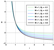
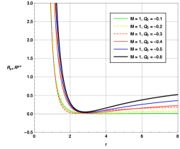
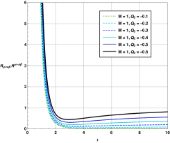
Figure 1: Variation of Ricci, Ricci squared and Kretschmann scalar w.r.t. $r$.

V Perturbations and Quasinormal modes

We have obtained the black hole solutions in $f(Q)$ gravity. Now, in this section, we shall deal with two types of perturbations in the black hole spacetime viz., massless scalar perturbation and electromagnetic perturbation. Here we shall assume that the test field i.e. scalar field or electromagnetic field has negligible impact on the black hole spacetime. To obtain the quasinormal modes, we derive Schrödinger-like wave equations for each case by considering the corresponding conservation relations on the concerned spacetime. The equations will be of the Klein-Gordon type for scalar fields and the Maxwell equations for electromagnetic fields. To calculate the quasinormal modes, we use two different methods viz., Bernstein spectral method and Padé averaged 6th order WKB approximation method.

Taking into account the axial perturbation only, one may write the perturbed metric in the following way [41]

$$ds^{2}=-\,|g_{tt}|\,dt^{2}+r^{2}\sin^{2}\!\theta\,(d\phi-p_{1}(t,r,\theta)\,dt-p_{2}(t,r,\theta)\,dr-p_{3}(t,r,\theta)\,d\theta)^{2}+g_{rr}\,dr^{2}+r^{2}d\theta^{2},$$ (37)

here the parameters $p_{1},p_{2}$ and $p_{3}$ define the perturbation introduced to the black hole spacetime. The metric functions $g_{tt}$ and $g_{rr}$ are the zeroth order terms, and they depend on $r$ only.

V.1 Scalar Perturbation

We start by taking into account a massless scalar field in the vicinity of the previously established black hole. Since we assumed that the scalar field’s effect on spacetime is negligible, the perturbed metric Eq. (37) may be reduced to the following form:

$$ds^{2}=-\,|g_{tt}|\,dt^{2}+g_{rr}\,dr^{2}+r^{2}d\Omega^{2}.$$ (38)

Now, one can write the Klein-Gordon equation in curved spacetime for this scenario as follows:

$$\square\Phi=\dfrac{1}{\sqrt{-g}}\partial_{\mu}(\sqrt{-g}g^{\mu\nu}\partial_{\nu}\Phi)=0.$$ (39)

This equation describes the quasinormal modes associated with the scalar perturbation. It is possible to decompose the scalar field as

$$\Phi(t,r,\theta,\phi)=\dfrac{1}{r}\sum_{l,m}\psi_{l}(t,r)Y_{lm}(\theta,\phi),$$ (40)

where we have used spherical harmonics and $l$ and $m$ are the associated indices. The function $\psi_{l}(t,r)$ is the radial time-dependent wave function. One can use this equation and Eq. (39) to have

$$\partial^{2}_{r_{*}}\psi(r_{*})_{l}+\omega^{2}\psi(r_{*})_{l}=V_{s}(r)\psi(r_{*})_{l},$$ (41)

here $r_{*}$ is expressed as

$$\dfrac{dr_{*}}{dr}=\sqrt{g_{rr}\,|g_{tt}^{-1}|}$$ (42)

which is known as the tortoise coordinate. $V_{s}(r)$ stands for the effective potential having the following explicit form:

$$V_{s}(r)=|g_{tt}|\left(\dfrac{l(l+1)}{r^{2}}+\dfrac{1}{r\sqrt{|g_{tt}|g_{rr}}}\dfrac{d}{dr}\sqrt{|g_{tt}|g_{rr}^{-1}}\right).$$ (43)

Here, $l$ is referred to as the multipole moment of the black hole’s quasinormal modes.

V.2 Electromagnetic Perturbation

Now we move to the electromagnetic perturbation, where one needs to utilise the standard tetrad formalism [72, 41] in which a basis $e^{\mu}_{a}$ is defined related with the black hole metric $g_{\mu\nu}$. This basis satisfies,

$$e^{(a)}_{\mu}e^{\mu}_{(b)} =\delta^{(a)}_{(b)}$$

$$e^{(a)}_{\mu}e^{\nu}_{(a)} =\delta^{\nu}_{\mu}$$

$$e^{(a)}_{\mu} =g_{\mu\nu}\eta^{(a)(b)}e^{\nu}_{(b)}$$

$$g_{\mu\nu} =\eta_{(a)(b)}e^{(a)}_{\mu}e^{(b)}_{\nu}=e_{(a)\mu}e^{(a)}_{\nu}.$$ (44)

One can express tensor fields in terms of this basis as shown below:

$$S_{\mu} =e^{(a)}_{\mu}S_{(a)},$$

$$S_{(a)} =e^{\mu}_{(a)}S_{\mu},$$

$$P_{\mu\nu} =e^{(a)}_{\mu}e^{(b)}_{\nu}P_{(a)(b)},$$

$$P_{(a)(b)} =e^{\mu}_{(a)}e^{\nu}_{(b)}P_{\mu\nu}.$$

The Bianchi identity of the field strength $F_{[(a)(b)|(c)]}=0$, in the case of the electromagnetic perturbation in the tetrad formalism results

$$\left(r\sqrt{|g_{tt}|}\,F_{(t)(\phi)}\right)_{,r}+r\sqrt{g_{rr}}\,F_{(\phi)(r),t} =0,$$ (45)

$$\left(r\sqrt{|g_{tt}|}\,F_{(t)(\phi)}\sin\theta\right)_{,\theta}+r^{2}\sin\theta\,F_{(\phi)(r),t} =0.$$ (46)

One can write the conservation equation as

$$\eta^{(b)(c)}\!\left(F_{(a)(b)}\right)_{|(c)}=0,$$ (47)

which can be further rewritten in terms of the spherical polar coordinates as

$$\left(r\sqrt{|g_{tt}|}\,F_{(\phi)(r)}\right)_{,r}+\sqrt{|g_{tt}|g_{rr}}\,F_{(\phi)(\theta),\theta}+r\sqrt{g_{rr}}\,F_{(t)(\phi),t}=0.$$ (48)

In the above expressions, a vertical rule and a comma denote the intrinsic and directional derivative with respect to the tetrad indices, respectively. Using Eq.s (45) and (46), and the time derivative of Eq. (48) one gets,

$$\left[\sqrt{|g_{tt}|g_{rr}^{-1}}\left(r\sqrt{|g_{tt}|}\,\mathcal{F}\right)_{,r}\right]_{,r}+\dfrac{|g_{tt}|\sqrt{g_{rr}}}{r}\left(\dfrac{\mathcal{F}_{,\theta}}{\sin\theta}\right)_{,\theta}\!\!\sin\theta-r\sqrt{g_{rr}}\,\mathcal{F}_{,tt}=0,$$ (49)

where $\mathcal{F}=F_{(t)(\phi)}\sin\theta.$ Using the Fourier decomposition $(\partial_{t}\rightarrow-\,i\omega)$ and field decomposition $\mathcal{F}(r,\theta)=\mathcal{F}(r)Y_{,\theta}/\sin\theta,$ where $Y(\theta)$ is the Gegenbauer function one can write Eq. (49) in the following form:

$$\left[\sqrt{|g_{tt}|g_{rr}^{-1}}\left(r\sqrt{|g_{tt}|}\,\mathcal{F}\right)_{,r}\right]_{,r}+\omega^{2}r\sqrt{g_{rr}}\,\mathcal{F}-|g_{tt}|\sqrt{g_{rr}}r^{-1}l(l+1)\,\mathcal{F}=0.$$ (50)

Using the definition $\psi_{e}\equiv r\sqrt{|g_{tt}|}\,\mathcal{F}$ and Eq. (42), it is possible to express Eq. (50) in the Schrödinger like form as

$$\partial^{2}_{r_{*}}\psi_{e}+\omega^{2}\psi_{e}=V_{e}(r)\psi_{e},$$ (51)

where the potential has the following explicit form:

$$V_{e}(r)=|g_{tt}|\,\dfrac{l(l+1)}{r^{2}}.$$ (52)

One may note that due to the behaviour of electromagnetic perturbation as shown above, the potential has a simple form and a comparison with Eq. (43) shows that an additional term is absent in the case of the electromagnetic perturbation. This comparison allows us to combine both of them in a compact form or representation as shown below:

$$V(r)=|g_{tt}|\left(\dfrac{l(l+1)}{r^{2}}+\dfrac{(1-s)}{r\sqrt{|g_{tt}|g_{rr}}}\dfrac{d}{dr}\sqrt{|g_{tt}|g_{rr}^{-1}}\right),$$ (53)

where the new parameter $s$ stands for spin. In the case of scalar perturbation, we have spin $s=0$ which reduces Eq. (53) to Eq. (43). In the case of electromagnetic perturbation, we have $s=1$, which results in the vanishing of the second term of the right-hand side of Eq. (53) and reduces it to Eq. (52).

V.3 Behaviour of Potentials

Here we shall briefly study the behaviour of the perturbation potential for the black hole defined above. Since the behaviour of the potential is highly associated with the quasinormal modes, one can have a preliminary idea related to the quasinormal modes from the potential behaviour.

One may note that the potential associated with an electromagnetic perturbation in the normal coordinate system does not depend on the model parameter $Q_{0}$, and it is completely identical to Schwarzschild’s case. However, in the case of quasinormal modes, we shall see $Q_{0}$ dependency due to the tortoise coordinates, which exhibit $Q_{0}$ dependency. Here, we shall only study the potential associated with scalar perturbation.

On the first panel of Fig. 2, we have shown the dependency of the scalar potential with respect to the multipole moment $l$. On the second panel, we show the impact of black hole mass on the scalar potential. One can see that the potential shows a different behaviour here which is basically due to smaller values of the parameter $Q_{0}$ and multipole moment $l$. We observe that the peak of the potential increases initially with an increase in the value of $M$. However, at a large distance $r$, a smaller value of $M$ corresponds to a large value of potential. To have a clear idea of how $Q_{0}$ impacts the scalar potential, we have plotted the potential for different values of $Q_{0}$ in Fig. 3. On the first panel, we choose smaller values of $Q_{0}$ and $l=3$. On the second panel, we choose large values of $Q_{0}$ with $l=1$. One can see that for $l=3$, on the first panel, we observe a normal behaviour of potential. Here, with an increase in the value of $Q_{0}$, potential decreases. While on the second panel, we observe peaks on the potential curve for small values of $r$. With an increase in $r$, the peaks vanish and the potential decreases to $0$ at $r=2$ and beyond this point, potential increases again. In this case also, for smaller values of $Q_{0}$, the potential has a larger value.

This analysis shows that the model parameter $Q_{0}$ has a significant impact on the potential behaviour. This suggests that the parameter $Q_{0}$ may have noticeable impacts on the quasinormal mode spectrum.

     

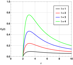
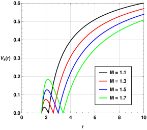
Figure 2: Variation of scalar potential $V_{s}(r)$ w.r.t. $r$. On the first panel, we have used $Q_{0}=-0.1$ and $M=1$. On the second panel, we have used $Q_{0}=-1.5$ and $l=1$.

     

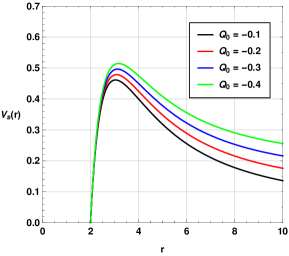
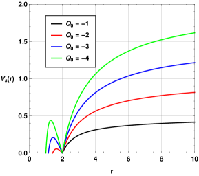
Figure 3: Variation of scalar potential $V_{s}(r)$ w.r.t. $r$. On the first panel, we have used $l=3$ and $M=1$. On the second panel, we have used $l=1$ and $M=1$.

V.4 Bernstein Spectral method for Quasinormal modes

The Bernstein spectral method is a numerical technique used to calculate quasinormal modes of black holes and other objects in GR and MGTs [73]. The Bernstein method is based on a spectral decomposition of the wave equation into a finite set of basis functions, which allows for highly accurate and efficient computation of quasinormal modes [73].

Such a method works by approximating the wave equation as a linear combination of basis functions, such as Bernstein polynomials or Chebyshev polynomials. The coefficients of this linear combination are then calculated using a collocation method, where the wave equation is evaluated at a set of discrete points in the domain of interest. By doing this, the wave equation is transformed into a matrix eigenvalue problem, which can be solved using standard numerical techniques such as the Arnoldi method or the Lanczos algorithm. The eigenvalues obtained in this way correspond to the complex frequencies of the quasinormal modes [73].

One of the key advantages of the Bernstein method is that it allows for a very high degree of accuracy, since the basis functions are globally defined and can be tailored to the specific problem at hand. Additionally, the method is computationally efficient, as it only requires the solution of a matrix eigenvalue problem, which can be done very quickly using specialized algorithms. The Bernstein method has been applied to a wide range of problems in both astrophysics and mathematical physics, including the calculation of quasinormal modes for black holes of different masses and spins, the computation of wave scattering by black holes and other objects, and the study of gravitational wave generation by binary black hole systems.

In summary, the Bernstein spectral method is a powerful and versatile numerical tool for the calculation of quasinormal modes in GR as well as MGTs and other areas of physics. Its combination of accuracy and efficiency make it a valuable tool for exploring the fundamental properties of black holes and other gravitational systems, and for the study of gravitational waves and their sources.

In this subsection, we shall implement the Bernstein spectral method [73] to obtain the quasinormal modes for the black hole system considered in this study. The method has been thoroughly discussed in Ref. [73]. In another recent study, this method has been revisited for asymptotically de Sitter, anti-de Sitter and flat black hole spacetimes. The corresponding quasinormal modes have been compared with those obtained using time domain analysis [74]. We define a compact coordinate $u$ as given by,

$$u=\frac{r_{h}}{r}.$$ (54)

We also define a wavefunction $\Psi(u)$ which is regular in the range $0\leq u\leq 1$, as

$$\Psi(u)=e^{i\Omega_{c}(\omega)/u}u^{\alpha(\omega)}(1-u)^{-i\Omega_{+}(\omega)}\psi(u),$$ (55)

where $\omega$ is the quasinormal frequency, and the other unknown parameters can be determined from the characteristic equations [74]. $\Omega_{c}$ and $\Omega_{+}$ satisfy the conditions

$$\frac{d\Omega_{c}}{d\omega}>0,\;\;\;\frac{d\Omega_{+}}{d\omega}>0.$$ (56)

The quasinormal boundary conditions representing incoming and outgoing waves are

$$\Psi\sim\left\{\begin{array}[]{rcl}e^{-i\omega r_{\star}},&r\to r_{+}&(r_{\star}\to-\infty),\\ e^{+i\omega r_{\star}},&r\to r_{c}&(r_{\star}\to+\infty).\end{array}\right.$$ (59)

Here $r_{\star}$ implies tortoise coordinate.

In our case, we express the wavelike equation in terms of $u=1/r$ so that $u=0$ and $u=1$ correspond to the event horizon and cosmological horizon respectively. After that, we factorise the equation to include $e^{i\Omega_{c}(\omega)/u}u^{\alpha(\omega)}(1-u)^{-i\Omega_{+}(\omega)}$ so that we obtain Eq. (55). This makes the new function regular at $u=0$ and $u=1.$ This is of course due to the inclusion of $u$ and $(1-u)$ in the function. Hence, both $u$ and $(1-u)$ play a very important role. More specifically, the new function at the boundaries becomes:

$$\Psi(u=0)=0\;\text{and}\;\Psi(u=1)=0,$$

which are both regular expressions providing mathematical feasibility to do the calculations numerically. The unknown terms such as $\Omega_{c}(\omega)$, $\alpha(\omega)$ and $\Omega_{+}(\omega)$ are obtained from the characteristic equations utilising series expansion near $u=0$ and $u=1$.

The function $\psi(u)$ is represented as a sum

$$\psi(u)=\sum^{N}_{k=0}C_{k}B^{N}_{k}(u),$$ (60)

in the above expression

$$B_{k}^{N}(u)\equiv\frac{N!}{k!(N-k)!)}u^{k}(1-u)^{N-k}$$ (61)

are known as the Bernstein polynomials. We use (55) in (41) and then a Chebyshev collocation grid [74],

$$u_{p}=\frac{1-\cos\frac{p\cdot\pi}{N}}{2}=\sin^{2}\frac{p\cdot\pi}{2N},$$ (62)

where $p=0,...,N$, to get a number of linear equations. Now the differential equation is simplified to the numerically solvable eigenvalue problem of a matrix of order 2 with respect to $\omega$. The solution gives the quasinormal frequencies, and by calculating the relevant coefficients $C_{k}$ and explicitly determining the polynomial (60), which roughly approximates the solution to the wave equation, one can get the complete solution of the problem. We compare the eigenfrequencies and related approximating polynomials for various values of $N$ in order to rule out the erroneous eigenvalues that emerge as a result of the polynomial basis’ finiteness. For this purpose, we follow Ref. [74] and calculate

$$1-\frac{|\langle\phi^{(1)}\;|\;\psi^{(2)}\rangle|^{2}}{||\psi^{(1)}||^{2}||\psi^{(2)}||^{2}}=\sin^{2}\alpha,$$ (63)

where $\alpha$ is the angle between two nearby eigenfunctions $\psi^{(1)}$ and $\psi^{(2)}$. We set a minimum cut-off $\alpha$ to determine the quasinormal modes from the eigenvalues. For better accuracy, one needs to consider a large value of $N$, which increases the computation time.

V.5 WKB method with Padé Approximation for Quasinormal modes

Apart from the above method, we shall use another well-established method known as the WKB method to estimate the quasinormal modes of the black hole considered in this study. We shall compare the results obtained from both methods to verify our findings.

The first-order WKB method or technique was introduced for the first time by Schutz and Will in Ref. [75]. Although this method can give approximate results of quasinormal modes, the error associated with this method is comparatively higher. For this reason, higher-order WKB methods have been implemented in the study of black hole quasinormal modes. The WKB method was upgraded to higher orders in Ref.s [76, 77, 78]. It was stated in Ref. [78] that the WKB technique may be improved by averaging the Padé approximations. Subsequently, it was discovered that this improved the findings of quasinormal modes with more precision [77]. The Padé averaged 6th-order WKB approximation approach will be used in this investigation.

Each table shows the quasinormal modes obtained from Padé averaged $6$th order WKB approximation method and Bernstein spectral method. The errors associated with the WKB method are represented by the rms error $\vartriangle_{rms}$ and $\Delta_{6}$, which is defined as [77]

$$\Delta_{6}=\dfrac{\vline\;\omega_{7}-\omega_{5}\;\vline}{2},$$ (64)

where the terms $\omega_{7}$ and $\omega_{5}$ represent quasinormal modes obtained from $7$th and $5$th order Padé averaged WKB method.

Table 1: Quasinormal modes of the black hole with $n=0$, $M=1$ and $Q_{0}=-0.1$ for the massless scalar perturbation.

$l$	Bernstein Spectral method	Padé averaged WKB	$\vartriangle_{rms}$	$\Delta_{6}$	$\Delta_{BW}$
$l=1$	$0.2929559-0.0601751i$	$0.294698\,-0.057859i$	$1.74634\times 10^{-6}$	$0.0000458873$	$0.965011\%$
$l=2$	$0.4848221-0.0624688i$	$0.485050\,-0.0622951i$	$7.66312\times 10^{-8}$	$9.15631\times 10^{-7}$	$0.0585984\%$
$l=3$	$0.6764037-0.0634309i$	$0.676414-0.0634246i$	$1.61704\times 10^{-8}$	$7.52219\times 10^{-8}$	$0.00178328\%$
$l=4$	$0.8682419-0.0638755i$	$0.868242-0.0638755i$	$4.59096\times 10^{-9}$	$1.99499\times 10^{-8}$	$0.0000082445\%$

Table 2: Quasinormal modes of the black hole with $n=0$, $M=1$ and $Q_{0}=-0.1$ for the electromagnetic perturbation.

$l$	Bernstein Spectral method	Padé averaged WKB	$\vartriangle_{rms}$	$\Delta_{6}$	$\Delta_{BW}$
$l=1$	$0.2655401-\ 0.0652171i$	$0.265539-0.065161i$	$0.0000177085$	$6.62115\times 10^{-6}$	$0.0205383\%$
$l=2$	$0.4676216-0.0647356i$	$0.467621-0.0647357i$	$7.32702\times 10^{-7}$	$4.67206\times 10^{-7}$	$0.000122958\%$
$l=3$	$0.6639979-0.0646406i$	$0.663998-0.0646407i$	$9.4691\times 10^{-8}$	$7.50012\times 10^{-8}$	$0.0000147967\%$
$l=4$	$0.8585978-0.0646038i$	$0.858598-0.0646038i$	$2.07449\times 10^{-8}$	$1.99993\times 10^{-8}$	$0.0000209396\%$

In Table 1, we have listed the quasinormal modes for the massless scalar perturbation with the model parameter $Q_{0}=-0.1$, the mass of the black hole $M=1$ and overtone number $n=0$. The term $\Delta_{BW}$ represents the percentage deviation of the quasinormal modes obtained via the Bernstein spectral method from the 6th order padé averaged WKB approximation method. Here in the Bernstein spectral method, a large value of $N$ increases the accuracy [79] but it needs a larger computation time. We have used $N=20,30,40$ and $60$ to compare the results for excluding the spurious eigenvalues. We compare the results by extracting the eigenvalues from each set that differ by an amount smaller than the specified cutoff value (around $0.01$). For each pair of eigenvalues meeting this criterion, we calculate the squared $\sin$ of the angle between their respective eigenfunctions using Eq. 63. When the $\sin$ value approaches zero or less than a cutoff value (we took it to be $1\times 10^{-10}$), it signifies that the eigenfunctions exhibit a negligible difference and approximate a common solution, possibly differing by a constant factor. By employing this technique, we effectively identify the dominant quasinormal modes. We see that excluding spurious eigenvalues and considering a suitable precision of numerical calculations allow us to choose small values of $N$ say around $40$ to obtain the desired accuracy instead of considering a large value such as $N=100$ which needs a higher computation time. One can see that for $l=1$, $\Delta_{BW}$ has a comparatively higher value. Apart from this, the errors associated with the Padé averaged WKB method are also higher. The percentage deviation, as well as the errors, decrease significantly as the multipole moment $l$ increases. The variation of these errors can be associated with the WKB method, which gives less significant results when $l-n$ is smaller. For both methods, it is clearly seen that the quasinormal frequencies and the damping rate increase with the value of the multipole moment $l$.

In Table 2, we have shown the quasinormal modes for electromagnetic perturbation for different $l$ values with $M=1$, $n=0$, and $Q_{0}=-0.1$. One can see that in this case also, the deviation term $\Delta_{BW}$ has higher values for smaller multipole moment $l$. As $l$ increases, the deviation, as well as the error terms, decreases noticeably.

From both Tables, it is clear that quasinormal frequencies have lower values for the electromagnetic perturbation than those obtained in the case of massless scalar perturbation. However, the decay rate or damping rate of GW is higher in the case of electromagnetic perturbation.

To see the effect of the model parameter $Q_{0}$ on the quasinormal modes, we have plotted the variations of quasinormal modes with respect to $Q_{0}$. On the left panel of Fig.4, we have plotted the real frequencies of quasinormal modes with respect to the nonmetricity scalar $Q_{0}$ for both massless scalar perturbation and electromagnetic perturbation. One can see that the scalar quasinormal mode frequency decreases significantly with an increase in the nonmetricity scalar $Q_{0}$. On the other hand, electromagnetic quasinormal frequencies increase slowly with an increase in the value of $Q_{0}$. Both types of frequencies approach each other when $Q_{0}$ is close to zero. One may note that $Q_{0}$ has more impact on the scalar quasinormal frequencies than the electromagnetic quasinormal frequencies. On the second panel of Fig.4, we have plotted the imaginary quasinormal modes with respect to the nonmetricity scalar $Q_{0}$. We observe that the damping rate or decay rate of gravitational waves increases with a decrease in the value of the scalar $Q_{0}$. The decay rate for the scalar perturbation is lower than that of electromagnetic perturbation for smaller values of $Q_{0}$ near $-1$. However, when $Q_{0}$ increases to $0$, the damping rate decreases and approaches zero. One may note that the variation of the damping rate with respect to $Q_{0}$ is nonlinear, unlike the case for real quasinormal modes, where the variation was linear for both types of perturbations.

     

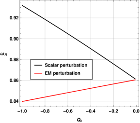
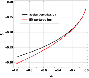
Figure 4: Variation of quasinormal modes with respect to model parameter $Q_{0}$ with $M=1$, $n=0$ and $l=4$ for massless scalar perturbation and electromagnetic perturbation.

Our analysis shows that the quasinormal mode spectrum carries the signature of nonmetricity, and in the near future, provided sufficient significant observational data is available, it might be possible to distinguish the scalar and electromagnetic quasinormal modes as well as the presence of nonmetricity in theory from a standard Schwarzschild black hole in GR.

VI Evolution of Scalar and Electromagnetic Perturbations on the Black hole geometry

In the previous section, we have numerically calculated the quasinormal modes and studied their behaviour with respect to the nonmetricity scalar $Q_{0}$. In this section, we shall deal with the time domain profiles of the scalar perturbation and electromagnetic perturbation. To obtain the time evolution profiles, we shall implement the time domain integration formalism [80]. For this purpose, we define $\psi(r_{*},t)=\psi(i\Delta r_{*},j\Delta t)=\psi_{i,j}$ and $V(r(r_{*}))=V(r_{*},t)=V_{i,j}$. Now, one can express Eq. (39) as

$$\dfrac{\psi_{i+1,j}-2\psi_{i,j}+\psi_{i-1,j}}{\Delta r_{*}^{2}}-\dfrac{\psi_{i,j+1}-2\psi_{i,j}+\psi_{i,j-1}}{\Delta t^{2}}-V_{i}\psi_{i,j}=0.$$ (65)

We set the initial conditions $\psi(r_{*},t)=\exp\left[-\dfrac{(r_{*}-k_{1})^{2}}{2\sigma^{2}}\right]$ and $\psi(r_{*},t)|_{t<0}=0$ (here $k_{1}$ and $\sigma$ are median and width of the initial wave-packet) and then calculate the time evolution of the scalar field as

$$\psi_{i,j+1}=-\,\psi_{i,j-1}+\left(\dfrac{\Delta t}{\Delta r_{*}}\right)^{2}(\psi_{i+1,j+\psi_{i-1,j}})+\left(2-2\left(\dfrac{\Delta t}{\Delta r_{*}}\right)^{2}-V_{i}\Delta t^{2}\right)\psi_{i,j}.$$ (66)

Using the above iteration scheme and choosing a fixed value of $\frac{\Delta t}{\Delta r_{*}}$, one can easily obtain the profile of $\psi$ with respect to time $t$. However, one should keep $\frac{\Delta t}{\Delta r_{*}}<1$ so that the Von Neumann stability condition is satisfied during the numerical procedure.

     

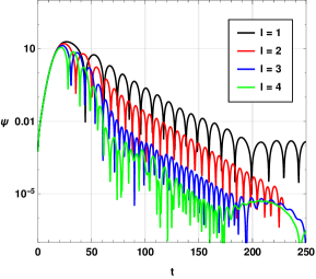
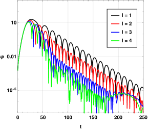
Figure 5: Time domain profiles with $M=1$, $n=0,Q_{0}=-0.1,$ for massless scalar perturbation (on first panel) and electromagnetic perturbation (on second panel).

     

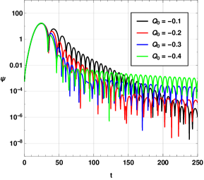
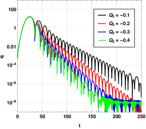
Figure 6: Time domain profiles with $M=1$, $n=0,l=2$ for massless scalar perturbation (on first panel) and electromagnetic perturbation (on second panel).

On the left panel of Fig. 5, we have shown the time domain profile for the scalar perturbation and on the right panel, we have shown the time domain profile for the electromagnetic perturbation with overtone number $n=0$, nonmetricity scalar constant $Q_{0}=-0.1$ and multipole number $l=1,2,3$ and $4$. We can see that the time domain profiles are significantly different for different values of multipole number $l$. For both cases, with an increase in the value of $l$, we observe an increase in the frequency. However, the decay rate of the time domain profile seems to increase for the scalar perturbation with an increase in the value of $l$ while for electromagnetic perturbation the variation is very small. Another interesting observation is that for $l=1$, both the scalar and electromagnetic time domain profiles have significantly different damping rate. The damping or decay rate seems to higher for the electromagnetic perturbation case than that of the scalar perturbation.

In Fig. 6, we have plotted the time domain profiles for scalar perturbation (on the left panel) and electromagnetic perturbation (on the right panel) with different values of the parameter $Q_{0}$ with overtone $n=0$ and multipole number $l=2$. One may note that the decay rate for the time profile of electromagnetic perturbation increases more rapidly with a decrease in the value of the parameter $Q_{0}$. The results obtained from the time domain profiles are consistent with the previous results of quasinormal modes.

VII Conclusion

In this work, we have studied the quasinormal modes of a static black hole in $f(Q)$ gravity. The black hole solution is obtained for the model $f(Q)=\underset{n}{\sum}a_{n}\left(Q-Q_{0}\right)^{n}$. We have considered two types of perturbations, viz., scalar perturbation and electromagnetic perturbation and obtained the corresponding potentials. We have seen that the potential in normal coordinates for the electromagnetic perturbation is identical to the potential corresponding to a Schwarzschild black hole. However, in the tortoise coordinate, the potential depends on the model parameter $Q_{0}$. As a result, both types of perturbations depend on the model parameter $Q_{0}$. To obtain quasinormal modes, we implement a newly introduced method known as Bernstein spectral method. To confirm the results obtained from this new method, we have considered well-known Padé averaged 6th-order WKB approximation method and found that the results obtained from the previous method stand in agreement with the results obtained from the higher-order WKB method.

The quasinormal modes vary significantly with the model parameter $Q_{0}$. It is found that for a nonzero $Q_{0}$, real quasinormal modes for scalar perturbation are always higher than those for electromagnetic perturbation. On the other hand, for smaller values of $Q_{0}$, the damping rate of gravitational waves associated with the scalar perturbation is always lower than that associated with the electromagnetic perturbation. We have also investigated the time domain profiles of the perturbations for different values of the model parameters. The results obtained from the time domain analysis agree well with the results provided by the numerical methods.

Since the black hole solutions are different in the $f(Q)$ nonmetricity theory from the solutions in other theories, the properties of black holes may be different in the framework of such theories. If any significant impacts are present in the generation and propagation of gravitational waves, recent detection of gravitational wave events can play a significant role in the study of the viability of such theories. Quasinormal modes are one of the interesting and widely studied properties of a perturbed black hole spacetime, and hence a detailed study of quasinormal modes from black holes in the framework of $f(Q)$ is necessary to understand the theory better. Our study shows that the black hole solution considered in the study can generate significantly different quasinormal modes from that of a Schwarzschild black hole [32]. Moreover, the quasinormal modes for the electromagnetic perturbation, as well as the scalar perturbation, are noticeably different for nonzero values of the model parameter $Q_{0}$.

The study of black holes and their properties in $f(Q)$ gravity is not very old, and still, there are very few studies incorporating various aspects of black holes in this theory. The study of different possible black hole solutions, especially in the presence of different promising surrounding relics, is necessary to understand the theory properly. Moreover, the thermodynamical aspects as well as quasinormal modes of black holes in $f(Q)$ are still left to be explored. Gravitational perturbation and related optical properties of the black hole, such as shadow, sparsity etc., are some probable future prospects of the study.

VIII ACKNOWLEDGMENTS

A. Ö. would like to acknowledge the contribution of the COST Action CA18108 - Quantum gravity phenomenology in the multi-messenger approach (QG-MM). A. Ö. would like to acknowledge networking support by the COST Action CA21106 - COSMIC WISPers in the Dark Universe: Theory, astrophysics and experiments (CosmicWISPers). DJG would like to thank Prof. U. D. Goswami for some useful discussions.

References

- [1] A. A. Starobinsky, Disappearing cosmological constant in f (R) gravity, JETP letters 86, 157–163 (2007).
- [2] A. De Felice and S. Tsujikawa, Construction of cosmologically viable f (G) gravity models, Phys. Lett. B 675, 1 (2009).
- [3] S. I. Nojiri and S. D. Odintsov, Dark energy, inflation and dark matter from modified F (R) gravity, arXiv:0807.0685 (2008).
- [4] W. Hu, I. Sawicki, Models of f (R) cosmic acceleration that evade solar system tests, Phys. Rev. D 76, 064004 (2007).
- [5] S.A. Appleby, R.A. Battye, Do consistent F (R) models mimic general relativity plus ?, Phys. Lett. B 654, 7 (2007).
- [6] S. Nojiri, S.D. Odintsov, Introduction to Modified Gravity and Gravitational Alternative for Dark Energy, Int. J. Geom. Methods Mod. Phys. 115, 4 (2007).
- [7] J. B. Jimenez, L. Heisenberg, and T. S. Koivisto, Coincident general relativity, Phys. Rev. D 98, 044048 (2018).
- [8] J. B. Jimenez, L. Heisenberg, T. S. Koivisto, and S. Pekar, Cosmology in geometry, Phys. Rev. D 101, 103507 (2020).
- [9] S. Capozziello et al., Cosmography in gravity, Phys. Rev. D 84, 043527 (2011).
- [10] Y. F. Cai et al., teleparallel gravity and cosmology, Rep. Prog. Phys. 79, 106901 (2016).
- [11] B. Li, T. P. Sotiriou, and J. D. Barrow, Large-scale structure in gravity, Phys. Rev. D 83, 104017 (2011).
- [12] S. Bahamonde, K. F. Dialektopoulos, C. Escamilla-Rivera, G. Farrugia, V. Gakis, M. Hendry, M. Hohmann, J. Levi Said, J. Mifsud and E. Di Valentino, “Teleparallel gravity: from theory to cosmology,” Rept. Prog. Phys. 86, no.2, 026901 (2023).
- [13] M. Adak, M. Kalay and O. Sert, Int. J. Mod. Phys. D 15, 619-634 (2006).
- [14] M. Adak and O. Sert, Turk. J. Phys. 29, 1-7 (2005).
- [15] M. Adak, Ö. Sert, M. Kalay and M. Sari, Int. J. Mod. Phys. A 28, 1350167 (2013).
- [16] M. Koussour et al., Anisotropic nature of space–time in gravity, Phys. Dark Universe 36, 101051 (2022).
- [17] M. Koussour et al., Thermodynamical aspects of Bianchi type-I Universe in quadratic form of gravity and observational constraints, J. High Energy Phys. 37, 15-24 (2023).
- [18] M. Koussour and M. Bennai, Accelerating Universe scenario in anisotropic cosmology, Chin. J. Phys. 79, 339-347 (2022).
- [19] M. Koussour et al., Late-time acceleration in gravity: Analysis and constraints in an anisotropic background, Phys. Ann. Phys. 445, 169092 (2022).
- [20] R. Lazkoz, F. S. N. Lobo, M. O. Banos, V. Salzano, Observational constraints of gravity, Phys. Rev. D 100, 104027 (2019).
- [21] S. Mandal, P. K. Sahoo, and J. R. L. Santos, Energy conditions in gravity, Phys. Rev. D, 102, 024057 (2020).
- [22] W. Wang, H. Chen, T. Katsuragawa, Static and spherically symmetric solutions in gravity, Phys. Rev. D 105, 024060 (2022).
- [23] F. D’Ambrosio, S. D. B. Fell, L. Heisenberg, S. Kuhn, Black holes in gravity, Phys. Rev. D 105, 024042 (2022).
- [24] Rui-Hui Lin and Xiang-Hua Zhai, Spherically symmetric configuration in gravity, Phys. Rev. D 103, 124001 (2021).
- [25] Zinnat Hassan, Sanjay Mandal, P.K. Sahoo, Traversable wormhole geometries in gravity, Forts. Phys. 69, 2100023 (2021).
- [26] G. Mustafa, Z. Hassan, P.H.R.S. Moraes, P.K. Sahoo, Wormhole solutions in symmetric teleparallel gravity, Phys. Lett. B 821, 136612 (2021).
- [27] A. Banerjee, A. Pradhan, T. Tangphati, F. Rahaman, Wormhole geometries in f(Q) gravity and the energy conditions, Eur. Phys. J. C 81, 1031 (2021).
- [28] M. Calza and L. Sebastiani, A class of static spherically symmetric solutions in f(Q) gravity, arXiv preprint arXiv:2208.13033 (2022).
- [29] O. Sokoliuk, Z. Hassan, P.K. Sahoo, A. Baransky, Traversable wormholes with charge and non-commutative geometry in the gravity, Ann. Phys. 443, 168968 (2022).
- [30] C. V. Vishveshwara, Stability of the Schwarzschild Metric, Phys. Rev. D 1, 2870 (1970).
- [31] W. H. Press, Long Wave Trains of Gravitational Waves from a Vibrating Black Hole, ApJ 170, L105 (1971).
- [32] S. Chandrasekhar and S. Detweiler, The Quasi-Normal Modes of the Schwarzschild Black Hole, Proc. R. Soc. Lond. A 344, 441 (1975).
- [33] C. Ma, Y. Gui, W. Wang, F. Wang, Massive scalar field quasinormal modes of a Schwarzschild black hole surrounded by quintessence, Cent. Eur. J. Phys. 6, 194 (2008) [arXiv:gr-qc/0611146].
- [34] D. J. Gogoi and U. D. Goswami, A New f(R) Gravity Model and Properties of Gravitational Waves in It, Eur. Phys. J. C 80, 1101 (2020) [arXiv:2006.04011].
- [35] D. J. Gogoi and U. D. Goswami, Gravitational Waves in Gravity Power Law Model, Indian J. Phys. 96, 637 (2022) [arXiv:1901.11277].
- [36] D. Liang, Y. Gong, S. Hou and Y. Liu, Polarizations of Gravitational Waves in Gravity, Phys. Rev. D 95, 104034 (2017) [arXiv:1701.05998].
- [37] R. Oliveira, D. M. Dantas, and C. A. S. Almeida, Quasinormal Frequencies for a Black Hole in a Bumblebee Gravity, EPL 135, 10003 (2021) [arXiv:2105.07956].
- [38] D. J. Gogoi and U. D. Goswami, Quasinormal Modes of Black Holes with Non-Linear-Electrodynamic Sources in Rastall Gravity, Physics of the Dark Universe 33, 100860 (2021) [arXiv:2104.13115].
- [39] J. P. M. Graça and I. P. Lobo, Scalar QNMs for Higher Dimensional Black Holes Surrounded by Quintessence in Rastall Gravity, Eur. Phys. J. C 78, 101 (2018) [arXiv:1711.08714].
- [40] Y. Zhang, Y.X. Gui, F. Li, Quasinormal modes of a Schwarzschild black hole surrounded by quintessence: electromagnetic perturbations, Gen. Relativ. Gravit. 39, 1003 (2007) [arXiv:gr-qc/0612010].
- [41] M. Bouhmadi-López, S. Brahma, C.-Y. Chen, P. Chen, and D. Yeom, A Consistent Model of Non-Singular Schwarzschild Black Hole in Loop Quantum Gravity and Its Quasinormal Modes, J. Cosmol. Astropart. Phys. 07, 066 (2020) [arXiv:2004.13061].
- [42] J. Liang, Quasinormal Modes of the Schwarzschild Black Hole Surrounded by the Quintessence Field in Rastall Gravity, Commun. Theor. Phys. 70, 695 (2018).
- [43] Y. Hu, C.-Y. Shao, Y.-J. Tan, C.-G. Shao, K. Lin, and W.-L. Qian, Scalar Quasinormal Modes of Nonlinear Charged Black Holes in Rastall Gravity, EPL 128, 50006 (2020).
- [44] S. Giri, H. Nandan, L. K. Joshi, and S. D. Maharaj, Geodesic Stability and Quasinormal Modes of Non-Commutative Schwarzschild Black Hole Employing Lyapunov Exponent, Eur. Phys. J. Plus 137, 181 (2022).
- [45] D. J. Gogoi, R. Karmakar, and U. D. Goswami, Quasinormal Modes of Non-Linearly Charged Black Holes Surrounded by a Cloud of Strings in Rastall Gravity, arXiv:2111.00854 (2021).
- [46] A. Övgün, İ. Sakallı and J. Saavedra, Quasinormal Modes of a Schwarzschild Black Hole Immersed in an Electromagnetic Universe, Chin. Phys. C 42, no.10, 105102 (2018) arXiv:1708.08331[physics.gen-ph]].
- [47] Á. Rincón and G. Panotopoulos, “Quasinormal modes of scale dependent black holes in ( 1+2 )-dimensional Einstein-power-Maxwell theory,” Phys. Rev. D 97, no.2, 024027 (2018).
- [48] G. Panotopoulos and Á. Rincón, “Quasinormal modes of regular black holes with non linear-Electrodynamical sources,” Eur. Phys. J. Plus 134, no.6, 300 (2019).
- [49] G. Panotopoulos and Á. Rincón, “Quasinormal spectra of scale-dependent Schwarzschild–de Sitter black holes,” Phys. Dark Univ. 31, 100743 (2021).
- [50] A. Rincon, P. A. Gonzalez, G. Panotopoulos, J. Saavedra and Y. Vasquez, Quasinormal modes for a non-minimally coupled scalar field in a five-dimensional Einstein–Power– Maxwell background, Eur. Phys. J. Plus 137, no.11, 1278 (2022) [arXiv:2112.04793 [gr-qc]].
- [51] P. A. González, Á. Rincón, J. Saavedra and Y. Vásquez, Superradiant instability and charged scalar quasinormal modes for (2+1)-dimensional Coulomb-like AdS black holes from nonlinear electrodynamics, Phys. Rev. D 104, no.8, 084047 (2021) [arXiv:2107.08611 [gr-qc]].
- [52] R. G. Daghigh and M. D. Green, Validity of the WKB Approximation in Calculating the Asymptotic Quasinormal Modes of Black Holes, Phys. Rev. D 85, 127501 (2012) [arXiv:1112.5397 [gr-qc]].
- [53] R. G. Daghigh and M. D. Green, Highly Real, Highly Damped, and Other Asymptotic Quasinormal Modes of Schwarzschild-Anti De Sitter Black Holes, Class. Quant. Grav. 26, 125017 (2009) [arXiv:0808.1596 [gr-qc]].
- [54] A. Zhidenko, Quasinormal modes of Schwarzschild de Sitter black holes, Class. Quant. Grav. 21, 273-280 (2004) [arXiv:gr-qc/0307012 [gr-qc]].
- [55] A. Zhidenko, Quasi-normal modes of the scalar hairy black hole, Class. Quant. Grav. 23, 3155-3164 (2006) [arXiv:gr-qc/0510039 [gr-qc]].
- [56] R. A. Konoplya and A. Zhidenko, Quasinormal modes of black holes: From astrophysics to string theory, Rev. Mod. Phys. 83, 793-836 (2011) [arXiv:1102.4014 [gr-qc]].
- [57] Y. Hatsuda, Quasinormal modes of black holes and Borel summation, Phys. Rev. D 101, no.2, 024008 (2020) [arXiv:1906.07232 [gr-qc]].
- [58] D. S. Eniceicu and M. Reece, Quasinormal modes of charged fields in Reissner-Nordström backgrounds by Borel-Padé summation of Bender-Wu series, Phys. Rev. D 102, no.4, 044015 (2020) [arXiv:1912.05553 [gr-qc]].
- [59] S. Lepe and J. Saavedra, Quasinormal modes, superradiance and area spectrum for 2+1 acoustic black holes, Phys. Lett. B 617, 174-181 (2005) [arXiv:gr-qc/0410074 [gr-qc]].
- [60] M. Chabab, H. El Moumni, S. Iraoui and K. Masmar, Phase Transition of Charged-AdS Black Holes and Quasinormal Modes : a Time Domain Analysis, Astrophys. Space Sci. 362, no.10, 192 (2017) [arXiv:1701.00872 [hep-th]].
- [61] M. Chabab, H. El Moumni, S. Iraoui and K. Masmar, Behavior of quasinormal modes and high dimension RN–AdS black hole phase transition, Eur. Phys. J. C 76, no.12, 676 (2016) [arXiv:1606.08524 [hep-th]].
- [62] M. Okyay and A. Övgün, Nonlinear Electrodynamics Effects on the Black Hole Shadow, Deflection Angle, Quasinormal Modes and Greybody Factors, J. Cosmol. Astropart. Phys. 2022, 009 (2022) [arXiv:2108.07766 [gr-qc]].
- [63] A. Övgün and K. Jusufi, Quasinormal Modes and Greybody Factors of Gravity Minimally Coupled to a Cloud of Strings in Dimensions, Annals of Physics 395, 138 (2018) [arXiv:1801.02555 [gr-qc]].
- [64] R. C. Pantig, L. Mastrototaro, G. Lambiase and A. Övgün, Shadow, lensing, quasinormal modes, greybody bounds and neutrino propagation by dyonic ModMax black holes, Eur. Phys. J. C 82, no.12, 1155 (2022) [arXiv:2208.06664[gr-qc]].
- [65] Y. Yang, D. Liu, A. Övgün, Z. W. Long and Z. Xu, Quasinormal modes of Kerr-like black bounce spacetime, [arXiv:2205.07530[gr-qc]].
- [66] Y. Yang, D. Liu, A. Övgün, Z. W. Long and Z. Xu, Probing hairy black holes caused by gravitational decoupling using quasinormal modes and greybody bounds, Phys. Rev. D 107, no.6, 064042 (2023) doi:10.1103/PhysRevD.107.064042 [arXiv:2203.11551 [gr-qc]].
- [67] A. Övgün, İ. Sakallı and H. Mutuk, Quasinormal modes of dS and AdS black holes: Feedforward neural network method, Int. J. Geom. Meth. Mod. Phys. 18, no.10, 2150154 (2021) [arXiv:1904.09509 [gr-qc]].
- [68] P. A. González, E. Papantonopoulos, Á. Rincón and Y. Vásquez, Quasinormal modes of massive scalar fields in four-dimensional wormholes: Anomalous decay rate, Phys. Rev. D 106, no.2, 024050 (2022) [arXiv:2205.06079 [gr-qc]].
- [69] D. J. Gogoi and U. D. Goswami, Tideless Traversable Wormholes surrounded by cloud of strings in f(R) gravity, JCAP 02, 027 (2023).
- [70] A. Chanda, and B. C. Paul, Evolution of primordial black holes in gravity with non-linear equation of state, Eur. Phys. J. C 82, 616 (2022).
- [71] J. B. Jiménez, L. Heisenberg, and R. S. Koivisto, Teleparallel palatini theories, J. Cosmol. Astropart. Phys., 2018, 08 (2018).
- [72] S. Chandrasekhar, The mathematical theory of black holes, Oxford University Press, Oxford (1992).
- [73] S. Fortuna and I. Vega, Bernstein Spectral Method for Quasinormal Modes and Other Eigenvalue Problems, arXiv:2003.06232 (2020).
- [74] R. A. Konoplya, A. Zhidenko, Bernstein spectral method for quasinormal modes of a generic black hole spacetime and application to instability of dilaton-de Sitter solution, arXiv:2211.02997 (2022).
- [75] B. F. Schutz and C. M. Will, Black Hole Normal Modes - A Semi analytic Approach, The Astrophysical Journal 291, L33 (1985).
- [76] S. Iyer and C. M. Will, Black-Hole Normal Modes: A WKB Approach. I. Foundations and Application of a Higher-Order WKB Analysis of Potential-Barrier Scattering, Phys. Rev. D 35, 3621 (1987).
- [77] R. A. Konoplya, Quasinormal Behavior of the D-Dimensional Schwarzschild Black Hole and the Higher Order WKB Approach, Phys. Rev. D 68, 024018 (2003) [arXiv:gr-qc/0303052].
- [78] J. Matyjasek and M. Telecka, Quasinormal Modes of Black Holes. II. Padé Summation of the Higher-Order WKB Terms, Phys. Rev. D 100, 124006 (2019) [arXiv:1908.09389].
- [79] P. Burikham, S. Ponglertsakul and L. Tannukij, Charged scalar perturbations on charged black holes in de Rham-Gabadadze-Tolley massive gravity, Phys. Rev. D 96, no.12, 124001 (2017) doi:10.1103/PhysRevD.96.124001 [arXiv:1709.02716 [gr-qc]].
- [80] C. Gundlach, R. H. Price and J. Pullin, Late time behavior of stellar collapse and explosions: 2. Nonlinear evolution, Phys. Rev. D 49, 890 (1994) [arXiv:gr-qc/9307010].