A variable star population in the open cluster NGC 6791 observed by the Kepler spacecraft

Abstract

We present the list of variable stars we found in the Kepler superstamp data covering approximately 9 arcminutes from the central region of NGC 6791. We classified the variable stars based on the variability type and we established their cluster membership based on the available Gaia Early Data Release 3 astrometry, by means of the Bayesian Gaussian mixture models. In total we found 278 variable objects, among which 17 binaries, 45 pulsators, 62 rotational and five unclassified variables are cluster members. The remaining 28 binaries, 25 pulsators, 83 rotational, four unclassified and nine unidentified variables are either not members or their membership is not established. In the case of eclipsing binaries we calculated the mid-times of eclipses and derived ephemerides. We searched for eclipse timing variation by means of the observed minus calculated diagrams. Only three objects show significant orbital period variation. Independently of a report published just recently by Colman et al. (2022) we found 119 new variables. We used isochrones calculated within the MIST project and derived the age (8.91 Gyr), average distance (4134 pc) and iron content [Fe/H] (0.26-0.28), of NGC 6791. Using the cluster members with membership probabilities greater than 0.9, we calculated the distance to the cluster of 4123(31) pc, which agrees with the result from our isochrone fitting.
Open clusters and associations : individual: NGC 6791 – binaries: general – Stars oscillations – Stars : rotation

1. Introduction

NGC 6791 has been first described as a metal rich cluster by Baade (1931) and listed as an old open cluster by King (1964). The authors provided no age estimations. Kinman (1965) presented a detailed comparative study of color – magnitude diagrams (CMD) of NGC 6791 along with other two open clusters, M 67 (4 Gyr) and NGC 188 (6.8 Gyr). From the first photometric observations in the B-V color, Harris and Canterna (1981) determined a reddening of E(B-V) = 0.13 mag. According to the recent studies NGC 6791 is 7 – 9 Gyr old (Chaboyer et al. 1999, Carraro et al. 2006, Basu et al. 2011), and it has a mass of around 4 000 M_⊙ (Kaluzny and Udalski 1992, Carraro et al. 2006, Platais et al. 2011, Tofflemire et al. 2014). The cluster is located $\sim$8000 pc from the Galactic center and 1000 pc above the Galactic plane. According to some hypotheses the cluster may have formed in the bulge of the Galaxy and radially migrated to its current location (Jilkova et al. 2012, Villanova et al. 2018). The distance to the cluster is approximately 3 614 pc, which was estimated for the first time by Stetson et al. (2003) from the de-reddened distance modulus of (m-M)${}_{0}\approx$12.79 mag. The authors derived E(B-V) = 0.09 mag. According to Villanova et al. (2018) NGC 6791 is a super metal-rich cluster with [Fe/H] = +0.3 – +0.4. Geisler et al. (2012) showed that NGC 6791 has multiple stellar populations, which makes the cluster chemically peculiar. NGC 6791 has an anomalous horizontal branch with a red clump (RC) region. Liebert et al. (1994) found a group of extreme horizontal branch members using spectrophotometry of blue targets observed by Kaluzny and Udalski (1992). The age of the cluster predicts that it should have a rich population of cooling white dwarfs, hence Bedin et al. (2005) observed the cluster using the Hubble Space Telescope up to m${}_{\mathrm{F606W}}\approx$ 28.5 mag. They found the white dwarf luminosity function to give a peak at 27.4 mag, which corresponds to an age of 2.5 Gyr. Such an estimate does not agree with the age derived from the main sequence (MS) or red giant branch (RGB) population (Chaboyer et al. 1999, Carraro et al. 2006). Thus far, these studies show the cluster is very unusual. A more detailed study is required to constrain the age and metal abundances for understanding the formation and evolution of NGC 6791. A clear picture of the cluster could be achieved by deriving an entire population of variable stars and analysis of components of the stars to find their ages and chemical abundances.

NGC 6791 has been a subject of extensive search for variable stars. Kaluzny and Udalski (1992) and Kaluzny and Rucinski (1993) did an extensive photometric survey finding 17 variable stars which includes 8 contact binaries, two blue stragglers and one binary consisting of a hot subdwarf B star. Rucinski et al. (1996) found three detached binaries and one cataclysmic variable (CV) star exhibiting a three day outburst. As a part of search for planets in stellar clusters, Mochejska et al. (2002) found 47 new low amplitude variable stars. The authors reported several BY Dra type and two outbursting CV stars, confirming the CV found by Rucinski et al. (1996). Mochejska et al. (2003) reported seven new variable stars with a long and periodic flux variation. Kaluzny (2003) found four new variable stars by reanalyzing archived data from Kaluzny and Rucinski (1993). A search for transiting events by giant planets reported by Bruntt et al. (2003) yielded 22 new low amplitude objects along with 20 previously known variable stars. Using a high precision time-series photometry, Hartman et al. (2005) detected 10 new variable stars including one $\delta$-Scuti type star and 8 contact binaries. Mochejska et al. (2005) detected 14 more variable stars and reported 9 eclipsing binaries. Using a high precision photometry in the Johnson V band, de Marchi et al. (2007) detected 260 variables in the cluster area, although not all stars are members of the cluster.

From the launch in 2009, for almost 10 years the Kepler spacecraft has served mankind by providing very precise and almost continuous photometric measurements (Koch et al. 2010). The Kepler has observed more than five hundred thousand stars during its entire mission time. The Kepler mission was completed in two phases. During the first mission, Kepler observed 0.25% of the sky in the direction of Cygnus and Lyra constellation for 1460 days. The mission was reborn as K2 (second mission) after the second reaction wheel failed. K2 mission made 80 day observing campaigns along the ecliptic equator, which lasted 1695 days (Howell et al. 2014). During both missions, the observations were obtained using two different exposures, 30 minutes for the long cadence (LC) and 1 minute for the short cadence (SC) mode (Koch et al. 2010, Borucki et al. 2010, Caldwell et al. 2010, Thompson et al. 2016). During the first mission, four open clusters were inside the Kepler field of view, NGC 6791, NGC 6819, NGC 6811 and NGC 6866. Two of the open clusters, NGC 6791 and NGC 6819, were observed by using the so-called LC superstamps.

Recently, Colman et al. (2022) presented light curves of KIC stars obtained from the Kepler superstamp data. The authors used an image subtraction method to derive light curves of all Kepler cataloged targets. They identified variability in 239 out of 5342 stars they extracted light curves of. The number of new variables is not given. We stress that our work has been performed simultaneously to, yet independently from, Colman et al. (2022) and contains additional analysis. By comparing our results with results of Colman et al. (2022), we have noticed that the authors applied a very strong detrending policy removing either eclipses or out-of-eclipse variations in binaries or variations in other objects that we claim to be variables.

In Section 2 of this paper, we present a brief description of the Kepler data and method used for obtaining the light curves of variable objects. In Section 3, we present a spectroscopic study of the variable stars found in this project using either archived spectra from public surveys or our own data. In Section 4, we describe the method of deriving the membership probabilities of our new variable star findings. In Section 5, we report individual variable star cluster members divided into variability classes. The field variable counterparts are listed in the Tables 5–8. In Section 6, we present the result of isochrone fitting.

2. Kepler Photometry

We downloaded the Kepler superstamp data of NGC 6791 from the Mikulski Archive for Space Telescopes (MAST). The data are 20 x 100 pixel boxes piled up in two contiguous 10 box stacks. The field of view of all pixels is 800 x 800 arcseconds and covers the most central part of the cluster. The superstamps data are collected in the LC mode. The pixel scale of an individual square pixel is 4 arcsec. The data have been collected over 1460 days and are split into 18 quarters.

We searched for a flux variation by extracting fluxes for all time stamps in individual pixels for each of the quarters Q 2 – 5. Then, a Fourier transform of the time-series data was performed in each pixel and each quarter separately. The pixels showing peaks (representing signal) in the amplitude spectra were selected. Signals that were identified with artifacts, either reported by Baran (2013) or those found in this project, were discarded. We combined all contiguous pixels showing the same signal and defined an optimal aperture of pixels. To keep the solar cells exposed to the sunlight, every quarter the spacecraft rolled 90 degrees, hence, with each quarterly rotation of the spacecraft, our targets landed on different CCD chips. This positioning caused different target images, and consequently, different optimal apertures (Bryson et al. 2010). Fortunately, every four quarters the images and apertures were the same, so we have defined the apertures only in four quarters, i.e. Q 2 – 5, and propagate them to the corresponding quarters (e.g. Q 2, 6, 10, 14). Next, using the optimal apertures for all targets showing flux variation we used PyKE software (Kinemuchi et al. 2012) to pull out the fluxes and correct them for instrumental artifacts by means of Co-trending Basis Vectors. Finally, using our custom scripts, we clipped the data at 4.5 sigma, detrended using spline fits, and normalized them to parts per thousand (ppt). The variable stars discovered in our work will be presented in Section 5.

3. Spectroscopy

We searched for spectra in the literature of all variables we detected. We found optical or infrared spectra for 111 objects in the archives of APOGEE (Ahn et al. 2014, Majewski et al. 2017), SDSS (Blanton et al. 2017), LAMOST (Zhao et al. 2012), ESO (Gilmore et al. 2012, Randich et al. 2013), and the HECTOSPEC (Fabricant et al. 2005) surveys. All spectra with T${}_{\rm eff}<15\,000$ K were modeled with interpolated local thermal equilibrium (LTE) synthetic spectra drawn from the BOSZ (Bohlin et al. 2017) spectral library to determine the fundamental atmospheric parameters. The BOSZ library was calculated for scaled solar metallicity with carbon and $\alpha$-element enhancement; therefore, individual abundance patterns cannot be investigated with our method.

Our fitting procedure (XTgrid; Németh et al. 2012) is based on a steepest-gradient chi-square minimizing method, which was originally developed to model hot stars. To improve its performance for cool stars, we added a grid-search preconditioning to the procedure. We step through a set of models to search for the best starting model for the steepest-descent part. Next, the descent part takes over in driving the fit and converges on the best solution. Once a convergence is achieved, the procedure explores the parameter errors by stepping through a set of points around the best solution. If a better solution is found during error calculations, then the procedure returns to the descent part, and hence pushing the solution towards the global minimum. XTgrid fits the radial velocity and projected rotation velocity of each spectra along with the stellar surface parameters, such as the effective temperature (T_eff), surface gravity ($\log$g) and abundances.

In addition, the procedure accesses photometric data from the VizieR Photometry Viewer, distance data from the Gaia EDR3 database, and extinction values from the NED online services. The spectroscopic surface parameters combined with these measurements allow us to reduce systematics and derive absolute stellar parameters, such as mass, radius, and luminosity. An anti-correlation is observed between T_eff and [Fe/H]. Fortunately, the spectral energy distribution (SED) helps in resolving this bias by restricting the T_eff. Another bias is observed in surface gravity, in particular below T_eff = 4 000 K. At such low temperatures, the spectrum is insensitive to the surface gravity. When the spectral coverage is very limited, we could not determine an accurate value for $\log$g. We do not report atmospheric parameters for such stars.

The archival spectroscopic data are very inhomogeneous. Consequently, high resolution spectra (e.g. obtained with ESO instruments) with a short wavelength coverage are more suitable for radial velocity measurements, while low resolution spectra (e.g. from the SDSS and LAMOST surveys) can provide more consistent atmospheric parameters, but less precise velocities. Some ESO spectra cover only 5 300-5 600 Å range at a resolution of R=20 000, and only weak spectral features are visible. For such spectra, at a relatively low signal-to-noise ratio (SNR), the fitting procedure increases the projected rotation above 100 km s^-1, which decreases the radial velocity accuracy. In general, low SNR spectra limit our analysis the most, while crowding in dense stellar fields and a limited spectral coverage affects the parameter determination.

4. Cluster membership

We used Gaia astrometry to determine the membership probabilities of all variable stars we found. We used five parameters, i.e. equatorial coordinates $\alpha$ and $\delta$, proper motions $\mu_{\alpha}$ and $\mu_{\delta}$, and parallax $\pi$ (further called five astrometric parameters). First, we adopted/estimated mean values of these parameters. The cluster center has been taken from Kamann et al. (2019) to be at $\alpha_{\rm 2000}$ = 19:20:51.3 and $\delta_{\rm 2000}$ = +37:46:26. Next, we downloaded Gaia Early Data Release 3 (EDR3) (Gaia collaboration et al. 2016, 2021) data for all stars within a tidal radius of 23 arcmin (Platais et al. 2011). The area contains 36 647 targets accessible to our analysis; however, we filtered out dubious targets with parallaxes to be negative or greater than 1 arcsec or relative uncertainties for any of the proper motion or parallax values to be greater than 50%. A cluster environment, particularly toward the center, is very dense, which can lead to unrealistic or imprecise estimates of these three parameters ($\mu_{\alpha}$, $\mu_{\delta}$, $\pi$). In addition, we limited our sample to targets for which the zero point offset corrections of parallax have been applied (Lindegren et al. 2021). After filtering and correcting for the parallax zero offset, we ended up with 11 466 targets.

To determine the membership probabilities, we used the Bayesian Gaussian Mixture Models (GMM) using scikit–learn python toolkit (Pedregosa et al. 2011). The GMM assumes each data point to be a combination of finite Gaussian functions, in which the number of these functions is determined using a variational Bayesian inference model with Dirichlet process prior (Ferguson 1973). We performed 10 000 iterations using the Expectation – Maximization algorithm (Dempster et al. 1977), and we derived membership probabilities for each target in our sample based on all five astrometric parameters. In the case of targets that we found variables in the superstamp area, we estimated their membership probabilities regardless of precision of their five astrometric parameters. If the uncertainties were larger than 50%, we considered corresponding parameters to be error-free, while the negative parallaxes were ignored and only four astrometric parameters were used.

To strengthen the probability, the radial velocity of individual stars can also be used, however they need to be corrected for the effects of binarity, rotation, and pulsations. Different instruments differ in instrumental calibration which often bias the radial velocity (RV) estimates. Since we did not conduct one single survey that could provide us with consistent RV estimations, we decided not to use RVs for the membership analysis. Since binarity and rotation affects the measurement of intrinsic motion, we expect the RVs will be random values and, as it will be seen in Section 5, the values in Tables 1–3, confirm our suspicion. We expected the most consistent estimates for single solar-like pulsators, since their oscillation motion on the surface is of a very small amplitude. In fact, in only three cases the RVs are far from the average cluster value (-47.46$\pm$1.08 km/s, Carrera et al. 2019), since the stars may belong to binary systems. On the other hand, RVs that are consistent indicate that the stars are likely single or the orbital motion (if any) is very slow or the spectra have been taken when both stars were aligned with the observer’s line of sight. The RVs of the solar-like stars that are unlikely to be members (Table 6) are not close to the cluster average and seem to confirm their field membership, unless they are in binaries.

5. A zoo of variable stars

In total, we found 278 variable objects in the superstamp area. Our sample contains cluster members as well as foreground and background stars. In Section 4, we provided details on a membership analysis. Our prime focus is on the members of NGC 6791. The non-members and objects with unknown membership status, as a consequence of a lack of the Gaia astrometry, are listed in the Table 5-8. Their variability is classified the same way as for the cluster members.

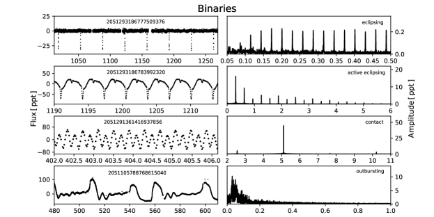
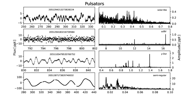
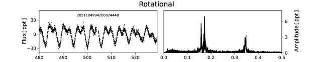
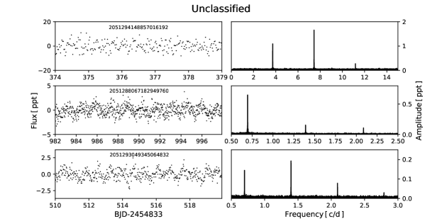
Figure 1: Examples of light curves and corresponding amplitude spectra of a zoo of variable stars in the open cluster NGC 6791.

Based on flux variations, we classified the stars into three main variability types, i.e. eclipsing, pulsating, and rotating stars. The first two types are further split into specific classes. Five stars remained unclassified. Their light curves show variations that we are unable to unambiguously identify as one of the three types listed. These objects show flux variations which can origin in e.g. a reflection effect, ellipsoidal variation or a rotation of a spotted star. These stars have typically low amplitude flux variations. In Fig. 1 we present examples of light curves and their corresponding amplitude spectra for each type and a selection of classes of variable stars we found.

5.1 Binary systems

We selected binary stars with sharp eclipses typical for semi- and detached systems. Some eclipsing systems show additional out-of-eclipse variation, which can be caused by a chromospheric activity, and we call them ”active” eclipsing. We identified contact systems, which are characterized by a continuous flux change and typical for W UMa stars. Another class contains outbursting stars, which we associate with binaries experiencing a rapid mass transfer causing sudden eruptions, e.g. novae, dwarf novae, nova-like variables. We stress that our classification is not based on radial velocities. Some of the stars may not be classified correctly, e.g. a smoothly continuous and small amplitude flux changes may be misidentified with rotational variables. However, the flux change over the course of observations is not modulated (see explanation in Section 5.3) or they can be long-period pulsating stars. In Fig. 2 we present the phased light curves of three stars that we consider new discoveries. The sample includes all the classes of binary stars we identified in the superstamp data. We found 17 binaries to be cluster members (Table 1), 28 binaries are field objects, including two binaries for which we could not establish membership due to the lack of Gaia astrometry data (Table 5). For binary systems their membership has been derived based on all five astrometric parameters. Majority of binaries in the cluster are main sequence (MS) stars with just two exceptions, assuming the position of the latter in the CMD is correct. Gaia EDR3 2051105720053889536 is a post-MS star on its early ascent of the red giant branch (RGB), while Gaia EDR3 2051293186783992320 is located below the RGB, which can be explained by an incorrect color index or pre-MS evolutionary status. Among the member counterparts, five are eclipsing, six active eclipsing, five contact, and one outbursting stars.

Table 1: List of binary stars that are cluster members.

Gaia EDR3	KIC	Porb	T0	G	CMD	HRD	Teff	$\log$g	RV	[Fe/H]	Ref
		[days]	[BJD]	[mag]			[K]		[km/s]
eclipsing
2051287203888386688	2436378 10L	8.531633(8)	2 454 969.2757(8)	19.031	MS+	–	–	–	–	–	–
2051288372129693440	2569175 X	43.499395(21)	2 455 041.61331(38)	18.383	MS	RGB	5 620(40)	3.517(18)	-65.8(4)	-0.67(9)	2∗
2051292980625561216	2437149 2S,6L	18.7986285(37)	2 454 971.02807(16)	17.480	MS	MS+MS	5 100(900)	4.5(4)	-80.9(9)	-0.25(25)	2∗
2051293083698347008	2437482 X	17.551175(14)	2 454 966.9452(7)	18.210	MS	RGB	4 860(50)	3.042(20)	-67.5(5)	-0.48(15)	1∗
2051293186777509376	2437041 X	34.859569(14)	2 454 979.90568(33)	18.055	MS	MS	6 360(40)	4.58(7)	-57.0(8)	-0.42(11)	2∗
active eclipsing
2051105342091761536	2437783 4L	7.453112(10)	2 454 964.7652(11)	18.391	MS	BS	7 160(50)	3.60(8)	-20.1(6)	-0.82(9)	2∗
2051105548255223680	2438490 4L	3.3157657(10)	2 454 967.85556(27)	17.887	MS+	HB	5 410(90)	2.87(7)	-62.2(12)	-0.68(15)	2∗
2051105784476572032	2438061 1S,12L	4.8858826(16)	2 454 965.01144(28)	17.721	MS	HB	5 220(30)	2.197(10)	-46.5(45)	0.42(22)	1∗
2051293186783992320	2437060 6L	3.1871038(8)	2 454 969.04204(21)	16.989	RGB	MS	5 270(20)	4.253(45)	-59.6(7)	-0.445(47)	1∗
2051294423734919552	2569494 1S,5L	1.5232747(12)	2 454 965.3339(7)	17.288	MS	MS	5 580(50)	4.06(6)	-116(8)	-0.36(11)	1∗
2051295351447975168	2570480 X	0.7349394(16)	2 454 964.9628(18)	19.340	MS+	HB	5 870(160)	2.34(11)	41.2(30)	-0.14(7)	2∗
contact
2051105543955885696	2438413 X	0.31754621(10)	2  454 964.63952(27)	18.281	MS	RGB	5 380(100)	3.347(38)	-34.70(13)	-0.631(46)	2∗
2051105720053889536	2438148 X	0.29468323(11)	2 454 964.79285(30)	16.612	RGB	–	–	–	–	–	–
2051291361416937856	2568950 X	0.3917614(15)	2 454 964.91341(33)	17.555	MS	MS/RGB	5 300(20)	3.926(20)	-39.50(10)	-1.131(26)	1∗
2051293324222974976	2569965 X	0.325587259(49)	2 454 964.71162(13)	17.510	MS+	MS	5 380(20)	4.46(8)	-63(6)	-0.36(8)	1∗
2051294114497255936	2569630 X	0.31265938(26)	2 454 964.7815(7)	16.964	MS	MS	5 620(50)	4,030(56)	-41(2)	-0.14(9)	1∗
outbursting
2051105788768615040	2438114 4L	32.27	–	18.192	blue of MS+	blue of MS	27 000(5 000)	7.3(6)	-34(25)	-1(1)	1∗

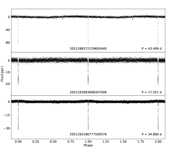
Figure 2: Phased light curves of three newly discovered binary star members of NGC 6791.

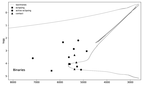
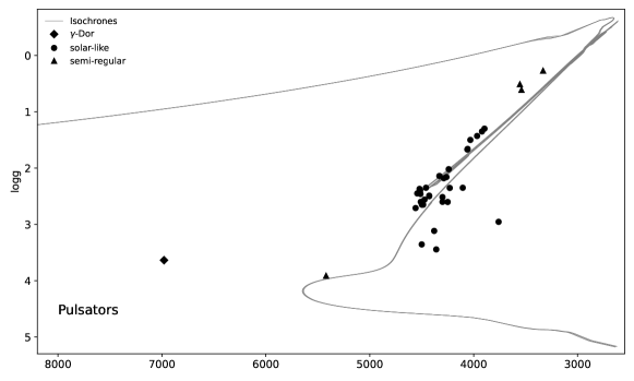
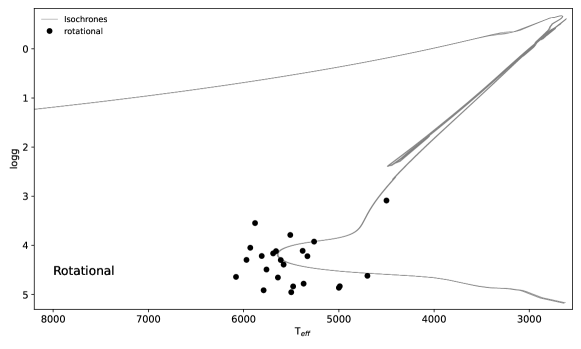
Figure 6: The T_eff–$\log$g diagram showing the cluster members with atmospheric parameters derived in this work. The top, middle and bottom panels show binary, pulsating and rotational stars, respectively. The isochrones represent the best MIST fits in T_eff and $\log$g coordinates.

Since the objects considered in this section are binaries, magnitudes and color indices used in the top panel of Fig. 3 and T_eff and $\log$g in the top panel of Fig. 6 (this figure will be explained in Section 6) may be averages of all components in a specific binary system and may not indicate a proper location of individual stars in the CMD. If the average location in the CMD diagram is in the well defined regions, e.g. MS or RGB, we can expect the components are of similar properties (or a secondary component is not detectable in our data), and the average is not far from single star values (unless the binary components are much different but the shift is only along a given evolutionary stage, e.g. along the RGB branch). If the location is outside those regions, e.g. below MS or RGB, then the individual components in a binary system are not alike, e.g. WD + MS, and the average will be somewhere between a WD track and the MS (as is the case for Gaia EDR3 2051105788768615040). For this same reason, the RV of binaries is typically different from the average RV of a cluster. We expect the orbital RV to be dominating. There are only one exception with the RV being close to the average cluster value. In the case of Gaia EDR3 2051105784476572032 the spectrum could have been taken during the eclipse or it is a spectroscopic single-line binary.

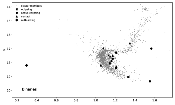
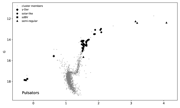
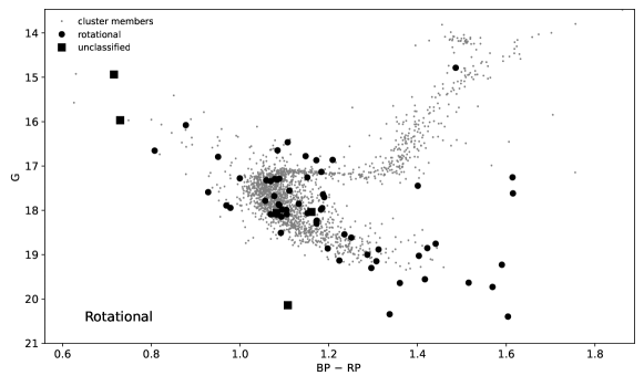
Figure 3: The color-magnitude diagram for NGC 6791. We listed variable stars such as binaries, pulsators and rotational cluster members in the top, middle and bottom panels, respectively. Unclassified stars are plotted in the bottom panel.

We estimated the mid-times of eclipses or, in the case of non-eclipsing systems, a minimum of a light variation by means of the method described in Kwee & van Woerden (1956). We used the mid-times to derive the ephemeris, i.e. a reference epoch, defined as the first mid-time in a given dataset, and an orbital period for each binary system we found. We provided estimates of these two parameters in Table 1 and Table 5. The exceptions are systems for which the data are very noisy, not allowing us to derive precise mid-times, and outbursting stars. For these systems we reported only rough estimates (arbitrarily adopted two decimal places for precision) of their orbital periods, derived from the Fourier amplitude spectra. The ephemerides were used to calculate the Observed - Calculated (O-C) diagrams to check on the orbital period variation. For most of the stars the O-C diagrams do not show any significant period variation. The exceptions are shown in Fig. 4. Gaia EDR3 2051294114497255936 (the top panel of Fig. 4) shows quite a large amplitude period variation with only one full cycle covered. These two O-C diagrams are constructed based on an average primary and secondary eclipses. Gaia EDR3 2051105342091761536 (the bottom panel of Fig. 4) shows cyclic variations of the orbital period derived solely from primary eclipses. To explain a periodic change an additional body in the system can be invoked. To test this hypothesis and, if confirmed, to constrain the parameters of those bodies, RV time-series data are required.

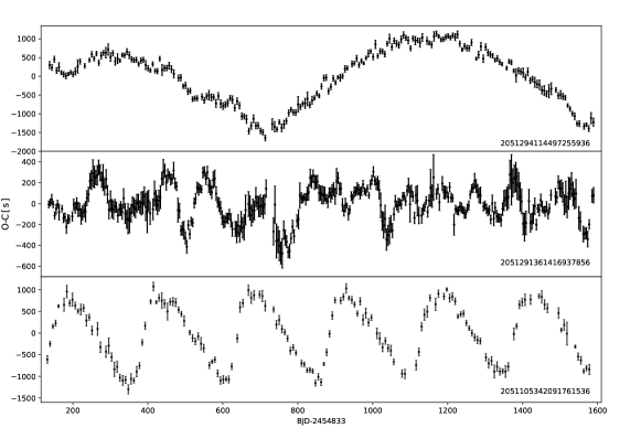
Figure 4: O-C diagrams for three binary systems that show variation of the orbital period.

5.2 Pulsators

We found 70 objects that show an intrinsic variability caused by stellar oscillations. We identified the following types of pulsators, i.e. $\delta$ Scuti and $\gamma$-Dor, solar-like along the RGB, RR Lyr, pulsating hot subdwarf B stars (sdBV) on the EHB, and semi-regular along the RGB and AGB. In Table 2 we show only the cluster member counterpart, while the field pulsators are listed in Table 6.

Among the cluster members we found one blue straggler, 36 solar-like pulsators (10 being RC objects, while 26 are still on the RGB), three sdBVs and five semi-regular giants. We analyzed the pulsation component in the solar-like counterpart, and the results will be published elsewhere. The analysis of the only three sdBVs we found in NGC6791 has been already reported by Sanjayan et al. (2022). Among sdBVs only Gaia EDR3 2051105509596144768 is a known binary star. The RV is likely influenced by orbital motion. The other two sdBVs also show different RVs from the cluster average, which may be an indication of their binary nature. Sanjayan et al. (2022) reported on the time-series spectroscopy (their Figure 4), which indicates a RV variation. The RVs of other pulsators we found to be members of NGC 6791 are close to the average value, with only a few exceptions. For instance, Gaia EDR3 2051293255503478528 shows a much faster motion, but the quality flag of the spectra suggests a possible contamination. We do not have resources to sort out these inconsistency cases. Perhaps the explanation of these cases is an additional RV component either of a binary or a rotational nature. In the case of other objects the RV confirms their membership and a single nature. We are aware that their spectra could have been taken while their orbital RV is negligible, but we consider it to be a less likely case. As in the case of binaries, the location of pulsators in the CMD (the middle panels of Fig. 3 and 6) may still be influenced by binary components.

Table 2: List of cluster members showing pulsations. See the caption of Table 1 for explanation. Ref 6 refers to Sanjayan et al. (2022).

Gaia EDR3	KIC	G	CMD	HRD	Teff	$\log$g	RV	[Fe/H]	Ref
		[mag]			[K]		[km/s]
$\gamma$-Dor
2051105479535706752	2438249 17L	15.573	BS	BS	6 980(90)	3.636(84)	-56.7(9)	-0.15(13)	2∗
solar-like
2051098710667044608	2297384 17L	14.204	RC	RC	4 512(91)	2.460(28)	-45.71(17)	0.400(7)	5
2051099260422933632	2437539 17L	14.545	RGB	RGB	4230(30)	2.353(10)	-39.9(4)	-0.57(7)	2∗
2051099329142406400	2437240 17L	14.648	RGB	RGB	4 380(70)	3.116(17)	-45.5(3)	-0.12(13)	2∗
2051104586182496000	2438462 12L	14.586	RGB	RGB	4 240(80)	2.020(23)	-45.71(37)	-0.39(7)	2∗
2051105135938204160	2437507 17L	14.032	RGB	RGB	4 262(80)	2.160(46)	-47.504(21)	0.400(7)	5
2051105135938218624	2437698 17L	14.191	RC	RC	4 521(93)	2.370(28)	-45.25(6)	0.400(8)	4
2051105239017444992	2437564 17L	14.226	RC	RC	4 515(99)	2.400(29)	-48.53(11)	0.400(9)	5
2051105342096702080	2437804 17L	14.110	RC	RC	4 459(97)	2.350(27)	-45.367(23)	0.400(9)	5
2051286795872609920	2436209 17L	14.802	RGB	RGB	4 498(103)	2.650(45)	-47.91(45)	0.400(9)	5
2051287002031072768	2437164 12L	14.157	RC	RC	4 300(50)	2.515(10)	-48.26(37)	-0.58(13)	2∗
2051287070750544128	2436900 17L	14.456	RGB	RGB	4 428(101)	2.500(45)	-47.92(8)	0.400(9)	5
2051287242549228032	2436608 10L	14.446	RGB	RGB	4 500(50)	2.254(35)	-45.5(15)	-0.07(7)	2∗
2051287311268703232	2436543 12L	14.120	RC	–	–	–	–	–	–
2051287311268706432	2436540 17L	14.856	RGB	RGB	4 473(104)	2.560(46)	-48.13(14)	0.400(10)	4
2051288067183227008	2436417 17L	14.104	RC	–	–	–	–	–	–
2051288135902691840	2436332 17L	14.302	RGB	RGB	4 360(60)	3.445(20)	-47.54(30)	-0.07(12)	2∗
2051288170262450816	2436458 17L	14.532	RGB	RGB	4 250(30)	2.602(10)	-46.36(30)	-0.24(11)	2∗
2051291228279110912	2435987 17L	14.529	RGB	RGB	4 428(98)	2.490(46)	-44(4)	0.400(9)	5
2051292877546340864	2437340 17L	13.462	RGB	RGB	4 058(82)	1.660(43)	-45.0(8)	0.300(9)	5
2051293083704792960	2437444 17L	13.998	RGB	RGB	4 105(66)	2.35(11)	-56(4)	0.12(6)	3
2051293118064539520	2437496 17L	13.069	RGB	RGB	3 920(67)	1.350(45)	-47.8(7)	0.300(7)	5
2051293118064542976	2437653 17L	15.090	RGB	RGB	4 559(97)	2.710(48)	-47(1)	0.400(8)	5
2051293152424246912	2436884 10L	13.476	RGB	RGB	4 061(83)	1.670(43)	-44.482(34)	0.300(9)	4
2051293186784001152	2437103 17L	14.378	RGB	RGB	4 500(50)	3.356(41)	-48.6(15)	0.002(92)	2∗
2051293221143724032	2436824 17L	14.478	RGB	–	–	–	–	–	–
2051293221143725952	2436814 17L	14.209	RGB	–	–	–	–	–	–
2051293255503469184	2436912 17L	14.181	RC	RC	4 330(90)	2.140(46)	-45.75(42)	0.300(8)	4
2051293255503478528	2437040 17L	14.158	RGB	RGB	3 760(50)	2.955(27)	-81.7(8)	0.003(10)	5 ∗
2051293319920668160	2569935 17L	13.065	RGB	RGB	4 032(65)	1.500(46)	-47.90(8)	0.400(6)	5
2051293599100902016	2570518 17L	14.683	RGB	RGB	4 509(89)	2.600(49)	-48.68(8)	0.300(7)	5
2051293977058270592	2436732 17L	14.135	RC	RGB	4 300(100)	2.60(7)	-44.9(2)	-0.36(8)	2∗
2051294045777739520	2569360 17L	14.093	RGB	RGB	4 287(86)	2.180(46)	-46.44(47)	0.300(8)	5
2051294114497261952	2569618 17L	14.797	RGB	RGB	4 486(103)	2.650(46)	-45.75(9)	0.400(9)	5
2051294213273828224	2569624 X	12.965	RGB	RGB	3 896(62)	1.300(45)	-44.98(7)	0.300(6)	5
2051294251936167424	2569204 11L	13.293	RGB	RGB	3 967(77)	1.430(43)	-47.909(11)	0.300(8)	5
2051297275593144192	2569055 17L	14.173	RC	RC	4 543(97)	2.450(29)	-46.881(12)	0.400(8)	5
sdBV
2051105509596144768	2438324 35S,12L	17.859	EHB	EHB	25 290(300)	5.510(43)	-90(3)	-2.62(11)	6
2051105754408746880	2437937 1S,1L	17.878	EHB	EHB	24 860(270)	5.348(52)	-75(6)	-2.46(12)	6
2051294183216739584	2569576 12S,5L	17.752	EHB	EHB	23 540(210)	5.311(35)	-28(4)	-2.73(23)	6
semi-regular
2051105101578558464	2438151 17L	15.655	RGB	MS	5 420(60)	3.912(19)	-50.0(15)	-0.10(9)	1∗
2051105616974709504	2438421 17L	12.246	AGB	AGB	3 555(57)	0.510(43)	-46.540(46)	0.200(8)	5
2051287002031070208	2437171 17L	12.394	AGB	AGB	3 540(56)	0.610(42)	-47.11(16)	0.300(8)	5
2051287173829740032	2436324 8L	12.373	AGB	AGB	3 332(53)	0.270(41)	-49.315(19)	0.200(10)	5
2051292976324527232	2437317 17L	14.939	RGB	–	–	–	–	–	–

5.3 Rotational Variables

We defined rotational type as stars showing modulated flux variation. Such variation is caused by the presence of migrating spots on the surface, which contribute to a flux modulation as a star rotates. The rotational variables can mimic other types of variability, e.g. ellipsoidal or contact binaries, and high-amplitude radially pulsating stars. We stress that our identification may not be ideal for rotational variable stars. We assumed that binaries show none or negligible modulation of a flux variation. This modulated variation can be verified by either a light curve shape or a profile of peaks in amplitude spectra. A complex profile indicates either period or amplitude change. Objects showing light curves with modulated flux variation have been classified as rotational variables.

We found a total of 145 rotational variables out of which 62 are cluster members and are listed in Table 3. The field counterpart is listed in Table 7. Likewise among binaries, there is no Gaia astrometry for four rotational variables and they are also listed in Table 7. We show the CMD location of members in the bottom panel of Fig. 3. The members occupy mostly the MS region, with three exceptions being the RGB objects and three exceptions being BS objects. Likewise in the case of binaries and pulsators, their true location may be influenced by binarity.

Table 3: List of cluster members showing rotational variability. See the caption of Table 1 for explanation.

Gaia EDR3	KIC	Period	G	CMD	HRD	Teff	$\log$g	RV	[Fe/H]	Ref
		[days]	[mag]			[K]		[km/s]
2051099015605500672	2297584 X	18.02	18.299	MS+	–	–	–	–	–	–
2051104757981275264	2438685 X	7.78	17.256	RGB	MS	5 500(50)	4.953(20)	-44.8(44)	0.47(15)	1 ∗
2051104891118311040	2437994 X	1.85	19.228	MS+	–	–	–	–	–
2051104891120796672	2437990 X	13.15	19.148	MS+	–	–	–	–	–	–
2051104959840285696	2437791 X	15.28	18.067	MS+	–	–	–	–	–	–
2051104964139549824	2437941 X	10.12	17.944	MS	–	–	–	–	–	–
2051104994200024448	2438113 X	5.80	17.288	MS	–	–	–	–	–	–
2051105097281783040	2438031 X	8.28	17.591	MS	MS	5 810(40)	4.216(34)	-62.3(23)	-0.158(47)	1 ∗
2051105131636983808	2437646 X	13.23	17.558	MS	–	–	–	–	–	–
2051105234715895552	2437707 X	11.00	17.867	MS	MS	6 080(30)	4.641(35)	-47.8(48)	0.60(14)	1 ∗
2051105273377206784	2437801 X	7.19	18.508	MS+	MS	5 380(70)	4.111(26)	-65.30(10)	-0.40(10)	1 ∗
2051105342091728384	2437761 X	11.81	19.001	MS	–	–	–	–	–	–
2051105372154852736	2437849 4L	11.02	16.863	MS	MS	5 260(50)	3.923(16)	-51.7(14)	-0.31(11)	1 ∗
2051105372154855552	2437944 X	1.96	18.543	MS+	–	–	–	–	–	–
2051105372157195264	–	2.45	19.556	MS+	MS	5480(50)	4.835(21)	-56(4)	0.45(17)	1 ∗
2051105578318626304	2438569 X	7.00	17.279	MS	MS	5 970(50)	4.295(20)	-69.2(15)	0.32(14)	1 ∗
2051105612675379968	2438390 X	3.80	17.987	MS	–	–	–	–	–	–
2051105685689315968	2438129 X	16.58	17.853	MS	–	–	–	–	–	–
2051105784484742144	2570443 X	2.20	17.643	MS	MS	5 610(50)	4.298(20)	-133.2(45)	-0.62(30)	1 ∗
2051105818833811584	2438344 X	7.74	18.616	MS+	–	–	–	–	–	–
2051105857492894592	2570649 X	13.36	17.293	MS	–	–	–	–	–	–
2051105921913036160	2570622 X	9.57	19.026	MS+	–	–	–	–	–	–
2051105926212896512	2570559 X	1.32	20.343	MS+	–	–	–	–	–	–
2051107055787471104	2438631 X	7.36	19.729	MS+	–	–	–	–	–	–
2051287002024520064	–	10.86	19.640	MS+	–	–	–	–	–
2051287066449451136	2436942 X	9.26	18.098	MS	–	–	–	–	–	–
2051287066449464064	2436959 X	2.65	18.852	MS+	–	–	–	–	–	–
2051287070744003456	2436969 X	7.92	19.132	MS+	RGB	4 500(50)	3.09(8)	-45.0(8)	-0.155(20)	2 ∗
2051287242549232384	2436767 X	12.32	17.309	MS	MS	5 690(50)	4.163(20)	-43.2(57)	0.148(33)	1 ∗
2051287895379273088	2436011 X	10.00	19.632	MS+	–	–	–	–	–	–
2051288372119657728	2569185 X	13.43	17.258	MS	MS	5 660(50)	4.117(34)	-97.9(35)	-0.08(10)	1 ∗
2051288376420896384	2569162 X	5.90	18.088	MS	–	–	–	–	–	–
2051291262638872192	2568864 X	14.42	17.618	MS	MS	5 370(30)	4.78(10)	-61.5(42)	0.58(27)	1 ∗
2051291503157017472	2568685 X	19.87	17.342	MS	–	–	–	–	–	–
2051292873245240192	2437350 X	16.82	17.885	MS	MS	5 790(50)	4.913(20)	-74.3(15)	0.13(8)	1 ∗
2051292911906089728	2437521 X	11.27	17.987	MS+	–	–	–	–	–	–
2051292946259301504	2437092 2L	3.20	18.145	MS+	MS	4 700(100)	4.619(50)	-78(1)	-1.87(6)	1 ∗
2051293014978876672	2437584 X	5.90	18.486	–+	–	–	–	–	–	–
2051293083704791040	2437354 8L	7.21	16.465	MS	MS	5 580(50)	4.391(20)	-55.6(8)	-0.413(46)	2 ∗
2051293113776412416	2437613 X	11.05	17.787	MS	–	–	–	–	–	–
2051293148133456896	2437062 X	8.82	17.133	RGB	–	–	–	–	–	–
2051293152424243968	2436909 X	12.00	16.778	MS	MS	5 640(40)	4.654(21)	-69.3(26)	-0.203(17)	1 ∗
2051293186783997056	–	9.63	18.232	MS+	–	–	–	–	–	–
2051293186784004096	2437238 X	4.00	16.079	BS	BS	5 880(30)	3.546(23)	-48.0(4)	-0.34(8)	2 ∗
2051293255503480320	2437079 X	5.81	16.794	BS	–	–	–	–	–	–
2051293289863230720	2437338 X	1.24	16.655	BS	–	–	–	–	–	–
2051293319934813184	2569984 X	12.50	17.704	MS	–	–	–	–	–	–
2051293358583014528	2569763 4L	8.29	16.648	MS	MS/RGB	5 510(20)	3.788(49)	-38.6(5)	-0.397(48)	2 ∗
2051293392942762240	2569825 X	0.48	18.754	MS+	MS	5 000(50)	4.86(15)	-86.3(7)	0.02(14)	1 ∗
2051293427302195584	2437884 X	3.23	16.871	MS+	MS	5 930(20)	4.048(26)	-43.9(3)	-0.44(10)	2 ∗
2051293530375009920	2570217 X	5.55	17.891	MS	MS	5 760(20)	4.49(7)	-62.4(23)	0.07(8)	1 ∗
2051293663519464192	2570420 X	19.96	17.951	MS	–	–	–	–	–	–
2051293977053182592	2436790 X	9.61	18.861	MS	MS	4 990(80)	4.832(25)	-169(3)	-0.356(15)	1 ∗
2051294007116759808	2569597 X	7.17	18.091	MS+	–	–	–	–	–	–
2051294148851985536	–	9.66	20.397	MS+	–	–	–	–	–	–
2051294148857020160	2569767 X	2.40	17.323	MS+	–	–	–	–	–	–
2051294217574157440	–	4.92	19.300	MS+	–	–	–	–	–	–
2051294251931077888	2569279 X	1.14	18.883	MS+	–	–	–	–	–	–
2051294281994746880	2569324 X	10.90	17.983	MS	–	–	–	–	–	–
2051294286296294528	2569334 X	6.29	17.447	MS	MS	5 330(20)	4.220(25)	-47.4(23)	0.15(8)	1 ∗
2051294797390943872	2569591 X	14.89	17.679	MS	–	–	–	–	–	–
2051296176081696768	2570281 12L	14.42	14.785	RGB	–	–	–	–	–	–

5.4 Unclassified and unidentified variables

In the case of nine objects, we were unable to unambiguously classify them according to the three types described above. The amplitude of a flux variation is low and it is not clear if the variation remains stable over time. The latter indicates that it is not unlikely these stars may be rotational variables. We leave a definite classification for further analysis, preferentially if based on better quality data. Five members of the cluster are listed in Table 4 and they are plotted in the bottom panel of Fig. 3, while four non-members are listed in Table 8.

While checking the pixel content we found signals in the amplitude spectra, associated with optical detections found in Pan-STARRS data (Chambers et al. 2016, Flewelling et al. 2020) survey that do not have any designations. We classified the signal to a proper variability type and estimated its period. We show the list of these unidentified objects in Table 9. Since the stars are not listed in the Gaia catalog, we are unable to estimate their membership. At three locations on the silicons (last three coordinates listed), we detected a signal in the amplitude spectra, however, we are unable to associate these coordinates with any optical objects in the Pan-STARRS survey. In addition, the last two signals listed may be of the same origin, though the coordinates are different. This result indicates that these three signals listed are residual signals of some other variable stars in the Kepler field of view that were spread over the silicons. We consider the signals detected at those three specific locations on the detector to be artifacts and not real sources.

Table 4: List of cluster members with unclassified variability. See the caption of Table 1 for explanation.

Gaia EDR3	KIC	Period	G	CMD	HRD
		[days]	[mag]
2051105269075634176	2437760 X	0.44	18.064	MS	–
2051288067182949760	2436421 8L	1.44	14.937	BS	–
2051291498855854208	2568724 X	0.63	20.141	MS+	–
2051293049345064832	2437745 X	1.43	15.968	BS	–
2051294148857016192	2569676 X	0.27	18.037	MS+	–

6. The distance and age estimation

We downloaded a grid of isochrones given in the Gaia photometric system from the MESA Isochrones and Stellar Tracks (MIST) project (Choi et al. 2016, Dotter 2016). The current version of MIST is 1.2. The MESA version 7503 was employed to calculate isochrones. We selected V/V_crit = 0. The grid covers age in a logarithmic scale between 9.8 and 10.3 with a step of 0.01, while [Fe/H] was between 0.20 and 0.45 with a step of 0.01.

At least 50$\%$ of the stars are expected to be in binary systems. The observed magnitude of a given target may include the flux contribution from all companions and not a single star, which shifts the position of the target in the CMD. Therefore, we excluded outlying stars where their positions in the CMD are uncertain. For the fit, we only kept the MS, RGB and RC stars. We included magnitude uncertainties as weights in the fit, which prevented the MS targets from over-fitting. The RC and RGB targets, even though less numerous, are brighter, and hence also remains significant in the fit.

The MIST synthetic isochrones are given in absolute magnitudes, and we selected no extinction. To account for a distance and a non-vacuum environment, in our fit, we included a shift (m-M) in the Gaia G magnitude and in B_p-R_p color. The best-fit isochrones point to a narrow range of age and [Fe/H]. The age is 8.91 Gyr, while [Fe/H] is between 0.26 and 0.28. The apparent distance modulus (m-M) equals 13.424, while E(B_p-R_p) from 0.165 to 0.176. We show the fits in Fig. 5. Based on the extinction curve from Cardelli et al. (1989), Bressan et al. (2012) showed a rough relation between extinction in the Gaia G band and E(B_p-R_p), which is A${}_{\rm G}\approx$2$\cdot$E(B_p-R_p). Taking the average of E(B_p-R_p) = 0.171 and using this relation, we derived A_G = 0.342 mag. Subtracting A_G from (m-M) we find the true distance modulus of 13.082, which gives the distance to the cluster of 4134 pc. We also derived distance from the parallaxes of the cluster members with probability membership at least 90% and the relative parallax uncertainty of smaller than 10%, which equals 4123(31) pc. The distance estimated from the isochrone fit lies well within the uncertainty of the distance estimations from the cluster parallax. The cluster age we derived from the isochrone fit is also comparable to the age reported by Choi et al. (2018).

To verify the correctness of the spectroscopic fits we also engaged isochrones in T_eff and $\log$g plane (HRD). We used the isochrones for the age and the average metallicity, which we derived from the isochrone fitting in the CMD. Then, we overplotted the isochrones with our variable stars from Tables 1-3, for which T_eff and $\log$g are listed. The column ’HRD’ in Tables 1-3 describes the location of a given star in the HRD. If the location agrees with the one in CMD, we can expect the spectroscopic fit is likely correct and we obtained an agreement for the majority of stars. It should be noted that the scatter in the HRD is larger, hence some objects may have not been allocated properly. There are clear exceptions, eight among binaries, two among pulsators and two among rotational variables. These cases should be treated with caution.

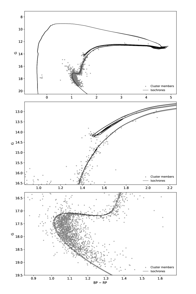
Figure 5: The color-magnitude diagram of NGC 6791, showing the best MIST isochrone fits. The top panel shows the overall diagram, while the middle panel shows the red clump region and the bottom panel shows the main-sequence region.

Table 5: List of binary stars that are not cluster members. See the caption of Table 1 for explanation. Targets with no astrometry available, hence with no membership established, are denoted in italic.

Gaia EDR3	KIC	Porb	T0	G	Teff	$\log$g	RV	[Fe/H]	Ref
		[days]	[BJD]	[mag]	[K]		[km/s]
eclipsing
2051104826700758016	2438661 X	196.34051(1)	2 455 037.21466(43)	16.449	–	–	–	–	–
2051105131638986752	–	23.878352(36)	2 454 967.0873(12)	19.782	–	–	–	–	–
2051107128803742336	2438562 X	10.406512(6)	2 454 965.58747(47)	19.369	6 220(130)	2.864(51)	-49(4)	-1.29(17)	2∗
2051287311268711168	2436579 X	9.287153(22)	2 454 971.1134(18)	19.613	–	–	–	–	–
2051291739386261248	2568780 X	3.5316020(11)	2 454 964.71245(25)	19.913	–	–	–	–	–
2051292907615354240	2437452 1S,17L	14.4699358(24)	2 454 974.81692(14)	17.286	6 170(50)	4.26(9)	-92.1(6)	-0.86(9)	2∗
2051293079414230912	2437505 10L	21.476420(11)	2 454 982.26244(40)	18.324	4 920(50)	3.25(6)	-19.6(30)	-0.25(19)	1∗
2051293118063233408	2437675 X	1.75	–	21.175	–	–	–	–	–
2051294629893394176	2569880 X	0.51323254(22)	2 454 964.60382(35)	17.866	–	–	–	–	–
active eclipsing
2051104586182512128	2438502 6S,16L	8.35905(26)	2 455 005.2748(14)	16.216	5 563(234)	4.17(37)	-14(5)	0.37(22)	3
2051104684959920896	2438464 X	0.43657907(7)	2 454 964.92853(13)	19.443	4 310(50)	4.169(20)	41(16)	-0.91(6)	1∗
2051286761512868992	2436203 X	2.06	–	14.328	–	–	–	–	–
2051288170257319808	–	3.7024382(14)	2 454 968.16622(31)	20.135	–	–	–	–	–
2051288372119654528	2569138 X	0.88305272(12)	2 454 964.71084(11)	19.205	–	–	–	–	–
2051293599094508032	–	2.8516350(19)	2 454 967.1274(6)	20.335	–	–	–	–	–
contact
2051105543955885312	2438471 X	0.27345629(34)	2 454 964.8195(11)	19.527	4 300(50)	3.92(7)	3.9(9)	-1.354(25)	1∗
2051288269040355584	2436044 X	0.24533697(21)	2 454 964.6646(7)	19.452	–	–	–	–	–
2051286417915483392	2297170 X	0.3664306(6)	2 455 002.6182(13)	17.797	–	–	–	–	–
2051287070750548736	2437038 17L	0.267678275(46)	2 454 964.58218(14)	16.149	–	–	–	–	–
2051291228279113216	2435971 17L	0.27182769(8)	2 454 964.81810(25)	16.276	–	–	–	–	–
2051291468797350528	2568971 17L	5.088522(10)	2454966.2350(17)	13.081	–	–	–	–	–
2051293530381417856	2570289 17L	0.279027932(31)	2 454 964.57880(1)	15.781	–	–	–	–	–
2051295076563264000	2570552 X	0.28417822(44)	2 454 964.5913(13)	20.279	–	–	–	–	–
2051295454527201792	2570460 X	0.2659879(15)	2 454 964.61531(47)	18.689	–	–	–	–	–
2051296313520692864	2708123 X	0.302184513(81)	2 454 964.69239(22)	17.742	–	–	–	–	–
2051297374371300992	2569082 X	0.33401898(23)	2 454 964.8252(6)	17.579	5 750(50)	4.052(15)	-38.30(54)	-1.069(20)	1∗
2051297477460338304	–	0.2690446(1)	2 454 964.7175(30)	20.838	–	–	–	–	–
outbursting
2051287203888388736	2436450 15S,12L	35.71	–	19.884	–	–	–	–	–

Table 6: List of pulsators that are not cluster members. See the caption of Table 1 for explanation.

Gaia EDR3	KIC	G	Teff	$\log$g	RV	[Fe/H]	Ref
		[mag]	[K]		[km/s]
$\delta$-scuti
2051098981244205056	2297728 1S,18L	9.929	6 888(25)	3.680(40)	-37(7)	0.272(22)	3
2051107369321426432	2570760 18L	13.459	–	–	–	–	–
solar-like
2051098710667526912	2297357 1L	12.115	–	–	–	–	–
2051099054264914048	2437622 12L	15.583	–	–	–	–	–
2051099329142404480	2437207 X	18.731	–	–	–	–	–
2051104105146054784	2297793 17L	13.626	4 085(81)	1.430(52)	-83.615(30)	-0.300(10)	5
2051104139506469760	2438094 17L	15.322	4 060(50)	1.11(15)	-84.7(6)	-1.14(8)	2∗
2051104861060304640	2437816 17L	13.958	4 229(77)	2.090(47)	0.400(7)	-47.27(9)	5
2051105720053903232	2438289 10L	14.384	–	–	–	–	–
2051105857492905600	2570715 7L	12.678	4 713(84)	2.330(36)	-3.30(7)	-0.200(7)	5
2051107369321441920	2570794 10L	15.158	–	–	–	–	–
2051286520994706432	2436457 18L	13.245	4 969(24)	3.015(39)	-19.14(4)	-0.422(22)	3
2051286933311578112	2436680 10L	15.187	–	–	–	–	–
2051288445140366464	2569078 10L	13.650	4 418(90)	2.290(49)	-5.428(56)	0.200(8)	5
2051291434437586304	2568912 8L	12.859	4 701(95)	3.01(6)	-7.122(55)	-0.100(8)	5
2051291567575397120	2568656 X	15.618	–	–	–	–	–
2051291571876502912	2568654 11L	13.140	4 301(83)	2.07(5)	-73.155(12)	0.100(8)	5
2051291674955780992	2568888 10L	14.131	4 387(100)	2.070(51)	-58.47(23)	-0.100(11)	5
2051291949833615104	2568575 5L	13.407	4 501(50)	2.55(8)	-2.26(4)	0.181(48)	3
2051293118064546944	2437692 15L	11.203	4 817(86)	2.610(38)	-12.780(24)	0.200(6)	5
2051293702180102144	2570002 X	13.628	–	–	–	–	–
2051294320655654912	2569137 10L	13.630	4 298(102)	1.71(6)	-194.10(44)	-0.800(16)	5
2051295282728537216	2570696 2L	13.620	4 461(80)	2.13(6)	-11.38(9)	-0.300(8)	5
RRLyr/BLBoo
2051294934839887872	2569850 X	20.426	–	–	–	–	–
semi-regular
2051105032859063424	2438242 X	16.817	4 511(99)	2.660(47)	-47.85(8)	0.400(9)	4

Table 7: List of rotational variables that are not cluster members. See the caption of Table 1 for explanation.

Gaia EDR3	KIC	Period	G	Teff	$\log$g	RV	[Fe/H]	Ref
		[days]	[mag]	[K]		[km/s]
2051098951180105088	–	1.33	20.929	–	–	–	–	–
2051099088624172928	2297416 X	2.66	20.201	–	–	–	–	–
2051099187404218752	2436945 X	4.58	16.735	–	–	–	–	–
2051104139500783744	–	0.64	20.943	–	–	–	–	–
2051104139505811328	2297846 X	13.40	14.901	–	–	–	–	–
2051104272645525760	2438284 X	2.63	19.629	–	–	–	–	–
2051104272645529472	–	1.53	20.277	–	–	–	–	–
2051104276944815744	2438272 18L	11.48	13.173	–	–	–	–	–
2051104586182508928	2438513 15S,17L	13.27	13.939	5 652(125)	4.51(8)	-35.74(33)	0.000(10)	5
2051104753679401728	2438740 X	0.42	19.653	–	–	–	–	–
2051104826696024832	–	1.06	20.370	–	–	–	–	–
2051104925480543616	2437773 X	0.51	19.083	6 070(110)	2.9(1)	8(4)	-0.54(15)	2∗
2051105062917626624	2437959 X	15.27	17.987	–	–	–	–	–
2051105067218772096	2437888 8L	10.34	14.730	6 120(80)	4.93(5)	16.42(37)	-0.39(12)	2∗
2051105067218785280	2438003 18L	0.70	13.025	7 132(30)	4.102(50)	3(10)	-0.22(3)	3
2051105135933158144	–	3.99	20.627	–	–	–	–	–
2051105239017448448	2437649 X	7.62	16.377	–	–	–	–	–
2051105273377200384	2437789 X	16.61	17.023	–	–	–	–	–
2051105303437700224	2437984 X	4.70	19.703	–	–	–	–	–
2051105307736986496	2437996 17L	14.61	13.887	5 753(37)	4.60(6)	-38(5)	0.104(35)	3
2051105410811376640	2438305 X	7.01	19.692	–	–	–	–	–
2051105823133141888	2438376 X	11.44	17.788	–	–	–	–	–
2051105926207653504	–	5.11	20.540	–	–	–	–	–
2051106063646757888	2438861 X	1.48	19.672	–	–	–	–	–
2051107124503872256	2438516 X	5.13	18.313	5 150(50)	4.773(27)	-36.9(15)	0.64(30)	1∗
2051107472400670720	2570846 17L	10.82	15.313	–	–	–	–	–
2051107541120138752	2570736 X	1.61	18.428	–	–	–	–	–
2051286997729896832	–	0.86	19.542	–	–	–	–	–
2051287066448488192	–	1.62	19.279	4 850(50)	4.871(40)	-112.4(1)	-0.15(12)	1∗
2051287139470009088	2436635 17L	1.17	15.989	4 445(291)	4.09(45)	-76(6)	-0.32(27)	3
2051287547485746432	2436206 X	8.25	17.626	–	–	–	–	–
2051288032823472128	2436274 X	4.58	18.220	–	–	–	–	–
2051288101537860992	–	3.39	20.539	–	–	–	–	–
2051288165961197952	2436416 X	3.99	19.859	–	–	–	–	–
2051288445135225472	2569015 X	1.32	20.103	–	–	–	–	–
2051290919041461632	2435889 X	14.47	16.670	–	–	–	–	–
2051291434437576320	2568884 X	10.50	18.224	–	–	–	–	–
2051291468792223104	–	7.37	20.190	–	–	–	–	–
2051291571876503424	2568672 X	18.09	16.477	–	–	–	–	–
2051292976335015296	2437180 X	4.07	17.907	–	–	–	–	–
2051292980625560448	2437292 X	5.51	18.356	–	–	–	–	–
2051292980625569792	2437234 17L	24.10	13.153	–	–	–	–	–
2051293014978879744	2437723 X	1.17	18.608	–	–	–	–	–
2051293014985313152	2437469 X	9.85	19.161	–	–	–	–	–
2051293014985313792	2437574 X	11.683	17.183	5 650(50)	4.5(8)	-45.0(3)	0.05(7)	1∗
2051293049338645504	–	1.97	20.310	–	–	–	–	–
2051293083704793856	2437359 17L	16.91	14.598	–	–	–	–	–
2051293152424251648	2436988 X	4.69	20.213	–	–	–	–	–
2051293221143720832	2436808 X	4.94	16.764	–	–	–	–	–
2051293255503475200	2436958 X	4.50	20.342	–	–	–	–	–
2051293289863227520	2437329 16L	11.67	15.925	–	–	–	–	–
2051293358577984768	–	1.55	20.049	–	–	–	–	–
2051293388640138880	–	8.48	20.028	–	–	–	–	–
2051293496015260416	2570182 X	1.99	18.719	–	–	–	–	–
2051293530375018112	–	4.27	20.832	–	–	–	–	–
2051293599094510848	2570536 17L	10.03	14.507	–	–	–	–	–
2051293839619440640	2570259 1S,1L	3.84	16.128	–	–	–	–	–
2051293908333956352	2570154 X	6.39	18.171	5 380(50)	4.004(20)	-68.6(36)	0.12(8)	1∗
2051293942698672000	2570258 X	7.40	16.852	–	–	–	–	–
2051293942698685056	2570313 X	1.39	19.449	–	–	–	–	–
2051293972756992384	2436621 X	7.58	18.758	–	–	–	–	–
2051293977053154688	2436734 X	1.59	20.187	–	–	–	–	–
2051294011418019072	2436852 X	3.31	18.871	–	–	–	–	–
2051294080137491968	2569421 X	13.51	18.689	–	–	–	–	–
2051294114495072896	–	3.54	20.960	–	–	–	–	–
2051294148851973888	2569675 X	5.24	20.253	–	–	–	–	–
2051294148857011712	2569737 14L	13.54	16.109	–	–	–	–	–
2051294492454406272	2569431 X	2.49	17.007	–	–	–	–	–
2051294664251895808	–	4.90	21.163	–	–	–	–	–
2051294728671468672	2569908 X	6.32	16.820	–	–	–	–	–
2051294831750674944	2569761 X	1.99	20.008	–	–	–	–	–
2051294870413630208	2569467 X	9.78	15.965	–	–	–	–	–
2051295007845559552	–	6.08	20.344	–	–	–	–	–
2051295007845583744	–	1.80	21.103	–	–	–	–	–
2051295488886958592	2570555 X	6.35	16.869	–	–	–	–	–
2051295557606451456	2570581 X	16.52	16.997	–	–	–	–	–
2051296652817037056	2707961 X	8.00	18.949	–	–	–	–	–
2051297516106367232	–	2.65	21.041	–	–	–	–	–
2051297962788050816	2707771 X	0.73	18.021	–	–	–	–	–
2051298031507519616	2707692 X	2.50	19.376	–	–	–	–	–
2051299474616582912	2707858 X	0.91	20.076	–	–	–	–	–
2051297275593155328	2569073 X	14.66	14.236	–	–	–	–	–
2051293255496998912	–	9.00	19.651	–	–	–	–	–

Table 8: List of unclassified variables that are not cluster members. See the caption of Table 1 for explanation.

Gaia EDR3	KIC	Period	G	Teff	$\log$g	RV	[Fe/H]	Ref
		[days]	[mag]	[K]		[km/s]
2051104654901977984	2438433 X	0.93	20.356	–	–	–	–	–
2051105307732052864	2438028 2L	0.06	20.639	3 470(50)	3.842(47)	-48.80(30)	0.09(10)	1∗
2051288337759883648	2436293 X	0.20	18.578	–	–	–	–	–
2051293736533447424	2570195 X	0.77	20.856	–	–	–	–	–

Table 9: A list of equatorial coordinates that are associated with superstamp pixels showing signal in their amplitude spectra. In the case of the last three positions listed, we found no optical objects that could be a source of the signal.

$\alpha_{\rm 2000}$	$\delta_{\rm 2000}$	Period	Type
[hh mm ss.ss]	[dd mm ss.s]	[days]
19 20 51.72	+37 47 45.4	1.10	rotational
19 20 53.56	+37 47 05.4	1.20	eclipsing
19 20 56.85	+37 47 43.2	2.40	rotational
19 21 13.06	+37 42 36.3	0.25	binary
19 20 31.99	+37 47 42.4	0.41	binary
19 20 45.84	+37 47 04.1	3.07	rotational
19 20 47.82	+37 42 18.2	0.68	rotational
19 21 03.71	+37 44 17.6	11.68	rotational
19 20 51.85	+37 39 51.5	9.21	solar-like
19 20 32.77	+37 43 23.8	0.15	binary
19 20 44.47	+37 40 51.5	5.73	rotational
19 20 46.46	+37 40 18.9	5.73	rotational

7. Summary

We presented a search for variable stars in the Kepler superstamp data. All available pixels were searched, by means of a Fourier amplitude spectrum, and a contiguous optimal aperture for each object that shows a significant flux variation were defined. The coordinates of these optimal apertures were matched with optical counterparts using Pan-STARRS. In total, we detected 278 variable stars. We cross-matched our variable star sample with those reported in the literature and found 16 variable stars reported by Kaluzny and Rucinski (1993), four by Rucinski et al. (1996), 23 by Mochejska et al. (2002), six by Mochejska et al. (2003), four by Kaluzny (2003), 15 by Bruntt et al. (2003), seven by Mochejska et al. (2005), one by Hartman et al. (2005) and 33 by de Marchi et al. (2007). We found 240 stars having KIC designations, out of which 140 stars do not have data delivered to the MAST. A variability of 119 stars was not known prior to our analysis. These stars are marked in bold in Tables 1-8, including the first nine objects listed in Table 9. Just recently, and independently of our work, Colman et al. (2022) reported light curves of stars with a KIC designation, however the authors did not specify which stars were found variables, only reporting a total number of 239 variables. Even accounting for this report, which is limited to the KIC stars only, we can consider 26 variable stars having no KIC designation (including seven objects marked in bold), to be new detections. No ground-based work on the detection of the variability of these 26 stars was reported, either.

Using Gaia EDR3 astrometry, we calculated the membership probabilities for all variable stars in our sample by applying Bayesian Gaussian mixture models. A star is considered to be a cluster member if the probability is higher than 50%. In total, we found 129 variable stars that are cluster members, 17 binary systems, 45 pulsators, 62 rotationally and five unclassified variables. The locations of these cluster variable stars in the CMD diagram were estimated and indicate the evolutionary status of cluster members. In the CMD, a majority of our variable stars are located in the MS. Solar-like pulsators are mostly located in the RGB and RC, while semi-regular variables are located in the RGB and AGB. In addition there are five BS and three EHB stars in the CMD.

In the case of binary systems, we estimated mid-times of eclipses and derived ephemerides. We calculated the O-C diagrams and checked for any orbital period variation. Only three binary systems show significant period variation, however its nature is not confirmed. The solar-like counterpart has been a subject of a detailed analysis of its pulsation content, and the results will be published elsewhere. The analysis of three sdBVs is already reported by Sanjayan et al. (2022). The rotational variables are not subject to our detailed analysis. This type of variables can be very useful toward gyrochronology.

We utilized public and archived spectra for 111 variable stars. Spectra for 64 stars were fitted with XTgrid, while for the remainder of the sample, we adopted the fit values from the surveys. We derived T_eff, $\log$g, [Fe/H] and RVs. Our spectral analysis was able to recover consistent stellar parameters from very diverse spectroscopic data. This consistency is reflected by the similar distribution of stars in the CMD and HRD. The most significant limiting factor on the parameter determination was the low SNR of some spectra, while the spectral coverage and crowding in dense fields played less significant roles. We found that the metallicity is not consistent among the cluster members and it is still unclear what causes it. If the inconsistency is real a possible explanation would be the presence of multiple stellar populations within the cluster as mentioned by Geisler et al. (2012). To confirm this hypothesis a uniform spectroscopic survey is required.

MIST isochrones were fit to our CMD comprised of cluster members, including our variable star population. From our best three fits, we derived a metallicity range of 0.26 to 0.28 and the age of NGC 6791 to be 8.91 Gyr. Our age estimate agrees with the values reported by e.g. Choi et al. 2018. The average distance estimate from the distance modulus is 4134 pc which overlaps with our independent estimate of 4123(31) pc we derived from the Gaia astrometry.

References

Ahn C. P. et al. 2014, ApJ, 211, 17
Baade W. 1931, Astronomische Nachrichten, 243, 303
Baran A. 2013, AcA, 63, 203
Basu S. et al. 2011, ApJ, 729, L10
Bedin L. R. et al. 2005, ApJ, 624, 45
Blanton M. R. et al. 2017, AJ, 154, 28
Bohlin, R. C. M,é,sz,á,ros, S., Fleming, S. W. et al. 2017, AJ, 153, 234
Borucki W. J. et al. 2010, Science, 327, 977
Bressan A. M. et al. 2012, MNRAS, 427, 127-145
Bryson S. T. et al. 2010, ApJ, 713, 97
Bruntt H., Grundahl F., Tingley B., Frandsen S., Stetson P. B., Thomsen B. 2003, A&A, 410,323
Caldwell D. A. et al. 2010, ApJ, 713, 92
Cardelli J. A. et al. 1989, ApJ, 345, 245
Carraro G., Villanova S., Demarque P., McSwain M. V.and Piotto G., BedinL. R., 2006, AJ, 643, 1151
Carrera R. et al. 2019, A&A, 623, A80
Chaboyer B., Green E. M., Liebert J. 1999, AJ, 117, 1360
Chambers K. C. et al. 2016, arXiv, 1612, 05560
Choi J., Dotter A., Conroy C., Cantiello M., Paxton B., Johnson B. D. et al. 2016,ApJ, 823, 102
Choi J. et al. 2018, ApJ, 863, 65
Colman I. L. et al. 2022, ApJS, 258, 39
de Marchi F. et al. 2007, A&A, 471, 515
Dempster A. P., Laird N. M., Rubin D. B. 1977, Journal of the Royal Statistical Society, 39, 1
Dotter A. 2016, ApJS, 222, 8
Fabricant D. et al. 2005, PASP, 117, 1411
Ferguson T. S. 1973, The Annals of Statistics, 1, 209
Flewelling H. A. et al. 2020, ApJ, 251, 7
Gaia Collaboration et al. 2016, A&A, 595, A1
Gaia Collaboration et al. 2021, A&A, 649, A1
Geisler D. et al. 2012, ApJ, 756, L40
Gilmore G. et al. 2012, The Messenger, 147, 25
Harris W. E. and Canterna R. 1981, AJ, 86, 1332
Hartman J. D., Stanek K. Z., Gaudi B. S., Holman M. J., McLeod B. A. 2005, AJ, 130, 2241
Howell S. B. et al. 2014, PASP, 126, 398
Jilkova L., Carraro G., Jungwiert B., Minchev I. 2012, A&A, 541, 64
Kaluzny J. and Rucinski S. M. 1993, MNRAS, 265, 34
Kaluzny J. and Udalski A. 1992, Acta Astronomica, 42, 29
Kaluzny J. 2003, Acta Astron., 53, 51
Kamann S., Bastian N. J., Gieles M., Balbinot E., Henault-Brunet V. 2019, MNRAS, 483, 2197-2206
Kinemuchi K. et al. 2012, Publications of the Astronomical Society of the Pacific, 124, 963
King I. R. 1964, Royal Greenwich Observatory Bulletins, 82, 106
Kinman T. D. 1965,ApJ,142,655
Koch D. G. et al. 2010, ApJ, 713, 79
Kwee K. and van Woerden H. 1956, Astronomical Institutes of the Netherlands, 12, 327
Liebert J., Saffer R. A., Green E. M. 1994, AJ, 107, 4
Lindegren L. et al. 2021, A&A, 649, A4
Majewski S. R et al. 2017, AJ, 154, 94
Mochejska B. J. et al. 2005, AJ, 129, 2856
Mochejska B. J., Stanek K. Z., Kaluzny J. 2003, AJ, 125, 3175
Mochejska B. J., Stanek K. Z., Sasselov D. D., Szentgyorgyi A. H. 2002, AJ, 123, 3460
N,é,meth, P., Kawka, A., Vennes, S. 2012, MNRAS, 427, 2180
Pedregosa F. et al. 2011, Journal of Machine Learning Research, 12, 2825
Platais I. et al. 2011, AJ, 733, 1
Randich S. et al. 2013, The Messenger, 154, 47
Rucinski S. M., Kaluzny J., Hilditch R. W. 1996, MNRAS, 282, 705
Sanjayan S. et al. 2022, MNRAS, 509, 763-777
Stetson P. B., Bruntt H., Grundahl F. 2003, PASP, 115, 413
Thompson, S, Fraquelli, D., Van Cleve, J., and Caldwell, D. 2016,KDMC, 10008,006
Tofflemire B. M., Gosnell N. M., Mathieu R. D., Platais I. 2014, AJ, 148, 61
Villanova S., Carraro G., Geisler D., Monaco L., Assmann P. 2018, ApJ, 867, 34
Zhao G.et al. 2012, A&A, 12, 7
Ahn C. P. et al. 2014, ApJ, 211, 17
Baade W. 1931, Astronomische Nachrichten, 243, 303
Baran A. 2013, AcA, 63, 203
Basu S. et al. 2011, ApJ, 729, L10
Bedin L. R. et al., 2005, ApJ, 624, 45
Blanton M. R. et al., 2017, AJ, 154, 28