Fermionic Adaptive Sampling Theory for Variational Quantum Eigensolvers

Abstract

Quantum chemistry has been identified as one of the most promising areas where quantum computing can have a tremendous impact. For current nisq devices, one of the best available methods to prepare approximate wave functions on quantum computers is the adapt. However, ADAPT-VQE suffers from a significant measurement overhead when estimating the importance of operators in the wave function. In this work, we propose algo, a method for selecting operators based on importance metrics solely derived from the populations of Slater determinants in the wave function. Thus, our method mitigates measurement overheads for adapt as it is only dependent on the populations of Slater determinants which can simply be determined by measurements in the computational basis. We introduce two heuristic importance metrics, one based on Selected Configuration Interaction with perturbation theory and one based on approximate gradients. In state vector and finite shot simulations, algo using the heuristic metric based on approximate gradients converges at the same rate or faster than adapt and requires dramatically fewer shots.

I Introduction

Quantum chemistry has been identified as one of the most promising areas where quantum computing can have great impact on industrial applications[1, 2, 3, 4]. However, current quantum hardware is subject to noise and error and thus algorithms such as quantum phase estimation remain intractable for current and near-term devices [5, 6]. Therefore, the research community has focused on developing algorithms suitable for an era of noise, error, limited qubits and limited quantum gates [7, 8]. A promising method to approximate electronic wave functions on quantum computers is the adapt algorithm, along with its variants, which has made tremendous progress towards this goal[9, 10, 11, 12, 13, 14]. Other adaptive algorithms include the Qubit Coupled Cluster method and the Iterative Qubit Coupled Cluster method [15, 16]. The adaptive approaches for estimating electronic wave functions contrast the static approaches such as Unitary Coupled Cluster Theory and its variants[17, 18, 19].

The adaptive algorithms have proven to converge to chemical accuracy with fewer parameters and more compact wave functions compared to that of the static algorithms. Thus, the adaptive algorithms may be more feasible for near-term applications. However, one of the primary challenges of adapt is the large measurement overhead incurred by estimating the importance metric for selecting relevant operators for the wave function [9]. Even estimating a single energy evaluation of a wave function through the sampling of expectation values may require significant measurement resources as was demonstrated in recent large-scale benchmarks [3]. For adapt, the importance metric for choosing operators from a predefined pool, $\mathcal{A}$, is the gradient of the energy. Therefore, the number of measurements necessary to rank the operators scales with the size of the pool, i.e. $\mathcal{O}(|\mathcal{A}|)$. Since $\mathcal{A}$ typically contains two-body operators, the size of the set of operators $|\mathcal{A}|$ scales as $\mathcal{O}(N^{4})$, where $N$ is a measure for the size of the chemical system.

In this work, we propose a method for selecting operators based on the populations of Slater determinants in the wave function in order to establish an importance metric for excitation operators. This is in stark contrast to adapt where the importance of operators is established using gradient measurements which requires the sampling of expectation values for each excitation operator. Sampling Slater determinants requires only the sampling of a single operator rather than $\mathcal{O}(N^{4})$ operators as in adapt. In fact, the required quantities for evaluating the proposed metric can be extracted from a measurement of the energy in vqe, a measurement that would in any case have to be performed.

For selecting operators, we are considering two metrics, one that is related to the approximate gradient used in adapt and a second one that is inspired by classical sci[20]. In classical sci, the determinants used to diagonalize the Hamiltonian are chosen using an importance metric typically based on a perturbation method[21, 22, 23, 24, 25]. Here we consider selecting operators based on second-order en perturbation theory[26, 27]. The methods are compared to adapt by calculating the ground state energies of two small molecules which are typically used in benchmarks, namely $\text{H}_{4}$ and LiH. The ground state energies are calculated using state vector (infinite shot) and finite shot simulations to investigate the performance of the methods both cases.

The paper is organized as follows. In Sec. II, we provide the theoretical background of adapt and sci. In Sec. III we provide the background for the scaling reduction in algo and derive the gradient-based and sci-based metrics. In Sec. IV, we provide a pseudo-algorithm for algo and provide the computational details of our calculations which we will present and discuss in Sec. V. Finally, we conclude with a summary and present some future research avenues in Sec. VI.

II Background

In this section, we will provide the background necessary for understanding the construction of our method in Sec. III, starting with adapt and followed by sci.

II.1 ADAPT-VQE

In adapt, an Ansatz is built by successively adding parametrized unitary operators acting on a reference state $\ket{\Phi_{0}}$, which is often taken as the hf ground state determinant. Thus, the adapt wave function in iteration $k$ of the algorithm can be expressed as

$$\ket{\Psi^{(k)}}=\prod_{\mu\in\mathcal{A}^{(k)}}e^{-i\theta_{\mu}\hat{A}_{\mu}}\ket{\Phi_{0}},$$ (1)

where $\mathcal{A}^{(k)}$ is the set of operators in the wave function at iteration $k$, $\hat{A}_{\mu}=\hat{\tau}_{\mu}-\hat{\tau}^{\dagger}_{\mu}$, with $\hat{\tau}_{\mu}$ being an excitation operator and $\mu$ enumerates the excitation. The excitation operators are chosen from a pool of operators, $\mathcal{A}=\{A_{\mu}\}$, based on an importance metric, $w(\hat{A}_{\mu},\ket{\Psi^{(k)}})$. In standard adapt, the importance metric is the gradient of the energy with respect to the parameter of the operator. The energy of the $k+1$st iteration may be written as

$$E^{(k+1)}=\langle\Psi^{(k)}|e^{i\theta_{\mu}\hat{A}_{\mu}}\hat{H}e^{-i\theta_{\mu}\hat{A}_{\mu}}|\Psi^{(k)}\rangle$$ (2)

such that

$$\begin{split}g_{\mu}&=\left.\frac{\partial E^{(k+1)}}{\partial\theta_{\mu}}\right|_{\theta_{\mu}=0}\\ &=i\langle\Psi^{(k)}|[\hat{A}_{\mu},\hat{H}]|\Psi^{(k)}\rangle.\end{split}$$ (3)

To evaluate this expression, adapt relies on measuring operators of the type $[\hat{A}_{\mu},\hat{H}]$, yielding a significant overhead in measurements to be performed.

II.2 Selected CI

In sci, determinants are selected iteratively by an importance metric in order to adaptively increase the subspace in which the CI eigenvalue problem is solved. One possibility for selecting determinants is based on perturbation theory[20]. In this paper, we consider en perturbation theory[26, 27]. en theory weights the importance of a Slater determinant $|D\rangle$ for extending a wave function $|\Psi^{(k)}\rangle$ in iteration $k$ as

$$\begin{split}E^{(k)}_{D}&=\frac{|\langle D|\hat{H}|\Psi^{(k)}\rangle|^{2}}{E^{(k)}-\langle D|\hat{H}|D\rangle}\\ &=\sum_{ij}\frac{c_{i}c_{j}^{*}\langle D_{j}|\hat{H}|D\rangle\langle D|\hat{H}|D_{i}\rangle}{E^{(k)}-\langle D|\hat{H}|D\rangle},\\ \end{split}$$ (4)

where the states $|D_{i}\rangle$ are Slater determinants and $c_{i}=\langle D_{i}|\Psi^{(k)}\rangle$ CI coefficients.

III FAST-VQE

In this section, we present a method for selecting operators solely based on the population of Slater determinants in the wave function by establishing importance metrics for excitation operators. This is in stark contrast to adapt where the importance of operators is established by measuring the expectation value of the non-diagonal gradient operators of Eq. (3). We start this section with a discussion of sampling populations of Slater determinants and diagonal Hamiltonian measurements in Sec. III.1 and then build the two metrics in Secs. III.3 and III.2.

III.1 Sampling populations of Slater determinants

A population of Slater determinants may, for example, be obtained from the energy evaluations in the vqe optimization or as a separate measurement. For separate measurements, given $\ket{\Psi^{(k)}}$, one may repeatedly perform measurements in the computational basis to obtain a bit string representation of determinants from $\ket{\Psi^{(k)}}$ in the hf basis. These measurements may be collected in a multi-set of determinants. The multi-set may be written as

$$S^{(k)}=\left\{|D_{i}\rangle,\langle D_{i}|\Psi^{(k)}\rangle\neq 0\right\},$$ (5)

where the frequency of each determinant $|D_{i}\rangle$ is proportional to $|c_{i}|^{2}$ and where the restriction is fulfilled by construction. With this set of determinants, we can build metrics suitable to assign importance weights to operators from an operator pool $\mathcal{A}$ based on the expected contribution to the wave function. In the following sections we will introduce two such metrics.
For energy measurements, the population of Slater determinants may be obtained through sampling the diagonal elements of the Hamiltonian. In vqe, the Hamiltonian is mapped to a qubit Hamiltonian,

$$\hat{H}=\sum_{a}h_{a}\hat{P}_{a},$$ (6)

where

$$\hat{P}_{a}=\bigotimes_{b}\hat{\sigma}_{b}^{\alpha},\quad\alpha\in\{x,y,z\},$$ (7)

denotes a product of Pauli operators. Consider a partitioning of the Hamiltonian $\hat{H}=\hat{H}^{z}+\hat{H}^{c}$ where $\hat{H}^{z}$ is diagonal, then we can express $\hat{H}^{z}$ as $\hat{H}^{z}=\sum_{a}h_{a}\hat{P}^{z}_{a}$, where $\hat{P}^{z}_{a}$ are products of Pauli-$z$ operators. We can then write an energy functional depending on the wave function parameters $\boldsymbol{\theta}$ in terms of this partitioned Hamiltonian as

$$\begin{split}E^{(k)}(\boldsymbol{\theta})&=\langle\Psi^{(k)}|\hat{H}^{z}+\hat{H}^{c}|\Psi^{(k)}\rangle\\ &=\sum_{a}h_{a}\langle\Psi^{(k)}|\hat{P}^{z}_{a}|\Psi^{(k)}\rangle+\langle\Psi^{(k)}|\hat{H}^{c}|\Psi^{(k)}\rangle\\ &=\sum_{ai}h_{a}|c_{i}|^{2}\langle D_{i}|\hat{P}^{z}_{a}|D_{i}\rangle+\langle\Psi^{(k)}|\hat{H}^{c}|\Psi^{(k)}\rangle\\ &=\sum_{i}h_{ii}|c_{i}|^{2}+\langle\Psi^{(k)}|\hat{H}^{c}|\Psi^{(k)}\rangle.\end{split}$$ (8)

Thus, we can perform measurements of diagonal Hamiltonian terms in the computational basis in order to sample Slater determinants $|D_{i}\rangle$ in $|\Psi^{(k)}\rangle$ with a probability that is proportional to $|c_{i}|^{2}$. Note that Eq. (8) is evaluated repeatedly in order to optimize the wave function parameters $\boldsymbol{\theta}$, e.g. using vqe, such that no additional cost is introduced to calculate Slater determinant populations.

III.2 Heuristic Gradient

To introduce the first heuristic importance metric, we start from $g_{\mu}$ in Eq.(3) which may be expressed as

$$\begin{split}g_{\mu}&=i\langle\Psi^{(k)}|\hat{A}_{\mu}\hat{H}-\hat{H}\hat{A}_{\mu}|\Psi^{(k)}\rangle\\ &=-i\langle\Psi^{(k)}|\hat{A}^{\dagger}_{\mu}\hat{H}+\hat{H}\hat{A}_{\mu}|\Psi^{(k)}\rangle\\ &=-2i\Re(\langle\Psi^{(k)}|\hat{A}^{\dagger}_{\mu}\hat{H}|\Psi^{(k)}\rangle)\\ &=-2i\sum_{ij}\Re(c_{i}^{*}c_{j}\langle D_{i}|\hat{A}^{\dagger}_{\mu}\hat{H}|D_{j}\rangle).\\ \end{split}$$ (9)

Then, dropping the off-diagonal part of the sum in Eq. (9) yields

$$\begin{split}\text{diag}(g_{\mu})&=2i\sum_{i}\Re(|c_{i}|^{2}\langle D_{i}|\hat{A}^{\dagger}_{\mu}\hat{H}|D_{i}\rangle)\\ &=2i\sum_{i}|c_{i}|^{2}\Re(\langle D_{i}|\hat{A}^{\dagger}_{\mu}\hat{H}|D_{i}\rangle).\end{split}$$ (10)

The manifold into which $\hat{A}^{\dagger}_{\mu}$ excites, $\{\langle D_{j}|\hat{A}^{\dagger}_{\mu},D_{j}\in S^{(k)}\}$, may be classically constructed. Such a manifold contains information on how the diagonal is connected to off-diagonal elements. To include that information in the final metric, a second sum over the determinants will therefore be introduced. In this regard, $S^{(k)}$ of Eq. (5) will be used directly since the number of occurrences of a determinant $\ket{D_{i}}$ in this multiset is proportional to $|c_{i}|^{2}$. Additionally, the second summation is introduced and all prefactors are removed, as the final ranking will not be dependent on constant factors. Thus, one obtains

$$\alpha_{\mu}=\sum_{D_{i}\in S^{(k)}}\sum_{D_{j}\in S^{(k)}}\Re(\langle D_{i}|\hat{A}^{\dagger}_{\mu}\hat{H}|D_{j}\rangle),$$ (11)

which concludes the construction of the first importance metric. This metric roughly corresponds to dropping the phases and prefactors from Eq. 9. Note that this expression can be evaluated classically once $S^{(k)}$ has been obtained. This importance metric will be denoted dsgn in the following.
In contrast to adapt, it is necessary to remove operators already used in the Ansatz, $\mathcal{A}^{k}$, from the operator pool, $\mathcal{A}$, in order to avoid using the same operator twice. However, to converge to the fci energy, it may be necessary to repeat operators in the Ansatz. Thus, whenever $\max_{\mu}(\alpha_{\mu})<\epsilon$, the operators $\mathcal{A}^{k}$ are added to the pool again.

III.3 Heuristic Selected CI

In order to introduce a second heuristically motivated metric, sci theory will be leveraged. In contrast to sci theory, which works with the determinants directly, it is required to build a metric that relates determinants and their frequencies in the sampling procedure to operators in order to gauge the effect of adding them to the Ansatz. In this section, such a metric will be constructed based on the en criterion from Eq. (4).

First, consider the adapt Ansatz in Eq. (1). The addition of a new operator corresponds to the multiplication of a new exponential which operates on all previous exponentials and the reference wave function. Thus, the contribution must be evaluated for all determinants already in $|\Psi^{(k)}\rangle$ and appropriately weighted. The construction of the heuristic operator metric based on determinants begins by noting that $\langle D_{i}|\hat{A}_{\mu}^{\dagger}=\langle D_{k}|$ is just another determinant or zero, establishing a connection between operators and determinants. From this, it would be possible to evaluate the contribution of $\hat{A}_{\mu}^{\dagger}$ by applying the en criterion in Eq. (4) directly using $D_{j}$ as the contribution to be evaluated. However, naively sampling the operator $H\ket{D_{k}}\bra{D_{k}}H$ comes at a significant cost with a scaling of $\mathcal{O}(N^{8})$. In order to make this manageable and to be able to evaluate this on a classical computer, the off-diagonal elements of the sum over $i$ and $j$ from Eq. (4) may be neglected. Furthermore, one must evaluate and sum such a metric for all the determinants an operator $\hat{A}_{\mu}^{\dagger}$ is able to create from the determinants in $|\Psi^{(k)}\rangle$, i.e., for practical implementations, all the determinants of the multi-set $S^{(k)}$. For representing the wave function in Eq. (4), the same approach as used to arrive at Eq. (11) will be used, i.e., a finite shot representation given the determinants collected in $S^{(k)}$ and using only the diagonal contributions.

This concludes the construction of the heuristic importance metric $\beta_{\mu}$, which may be written as

$$\begin{split}\beta_{\mu}&\coloneqq\sum_{D_{i}\in\mathcal{S}^{(k)}}\sum_{D_{j}\in\mathcal{S}^{(k)}}\frac{|\langle D_{i}|\hat{A}^{\dagger}_{\mu}\hat{H}|D_{j}\rangle|^{2}}{E^{(k)}-\langle D_{i}|\hat{A}^{\dagger}_{\mu}\hat{H}\hat{A}_{\mu}|D_{i}\rangle}.\end{split}$$ (12)

This importance metric will be denoted as enlm. Note that also for this metric, we need to remove used operators from $\mathcal{A}$, as explained in Sec. III.2.
The importance metrics in Eqns. (11) and (12) both use the operator $\hat{A}^{\dagger}\hat{H}$ for the evaluation of the importance of an operator $\hat{A}_{\mu}$ when improving the wavefunction in the next iteration. From a set of determinants, it is trivial to evaluate the expectation values for this operator on a classical computational resource with polynomial scaling in the number of electrons and orbitals.

IV Computational details

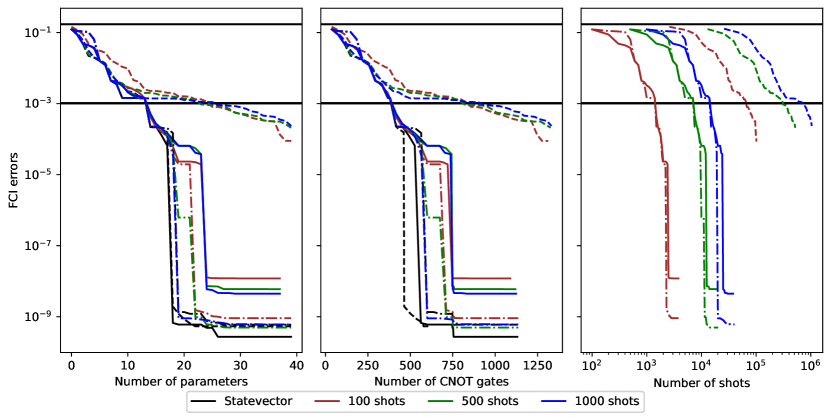
Figure 1: Convergence of adapt (dashed), enlm (full) and dsgn (dotted) with respect to the number of parameters (left), CNOT gates (middle) and the total number of shots (right) at a given precision of the obtained wave function for a linear $\text{H}_{4}$ chain at 1.5 Angstrom separation between subsequent atoms.

In this section, the algorithms and computational details of the calculations will be reviewed, starting with a description of the algorithm in Sec. IV.0.1, a description of the choice of operator pool in Sec. IV.0.2 and finally with a description of the numerical experiments in Sec. IV.0.3

IV.0.1 Review of algorithms

The general algorithm for adapt and algo is presented in Alg. 1. Note that the major difference between these methods is the skipping of lines 7-10 for adapt. For adapt, the importance metric reads $w(\hat{A}_{\mu},\ket{\Psi^{k}})_{\textrm{ADAPT-VQE}}=g_{\mu}$, while for algo we are using the importance metrics introduced earlier, i.e., $w(\hat{A}_{\mu},~{}|\Psi^{(k)}\rangle)_{\textrm{HG}}~{}=~{}\alpha_{\mu}$ and $w(\hat{A}_{\mu},~{}|\Psi^{(k)}\rangle)_{\textrm{HSCI}}~{}=~{}\beta_{\mu}$.

Note that modifications for adapt, for example TETRIS-ADAPT-VQE[13], which adds more than one operator per iteration, are also applicable to algo. However, we do not expect the relative performance of the algorithms to differ when using these types of improvements since the importance metrics are identical for the operators despite adding more than one operator per iteration. Thus, standard implementations for adapt and algo are used.

IV.0.2 Choice of operator pools

In general, any type of operator pool may be utilized. However, one-body and two-body excitation operators are enough to parametrize an FCI wave function [28]. Since the quantum gates required for implementing $N$-body excitation operators increase rapidly with $N$, operator pools are typically restricted to one-body and two-body excitation operators. According to Ref. [28] all possible many-body operators may be decomposed as one-body and two-body excitation operators, specifically as infinite sequences of one- and two-body particle-hole operators. Particle-hole excitation operators are excitation operators which annihilate electrons in occupied spin-orbitals in the hf reference state and create electrons in virtual spin-orbitals of the hf reference. In the original formulation of adapt, the operator pool consisted of general excitations (particle-hole excitations and excitations within the pure virtual-virtual or occupied-occupied blocks) in the jw encoding[29]. The resulting operator pools determine the scaling and convergence of the procedures. Additionally, rather than using these physically motivated operator pools, one can build operator pools that are computationally motivated. For example, several approximations have been suggested such as qeb_adapt_vqe [11] and spin-adapted ADAPT-VQE [30]. Recently, operator pools which consider qubit-space operators were suggested [10]. In this article, we will use particle-hole excitation operators in the qeb_adapt_vqe encoding since the primary task of this paper is to investigate importance metrics and not the operators themselves.

IV.0.3 Systems and details

Benchmarks of the algorithms are performed by calculating the ground state energy for $\text{H}_{4}$ and LiH which are typically used to benchmark adapt algorithms [9, 17, 16]. In these calculations, the STO-3G basis set were used. The molecular integrals were obtained using PySCF. The optimization of the wavefunction parameters in vqe is calculated with the L-BFGS-B method as implemented in Qiskit [31]. For all molecules, four types of calculations were performed, one state vector simulation and three simulations with finite sampling (100, 500 and 1000 shots per expectation value estimation). The optimization of the wave function in the vqe was performed using statevector simulations since we are restricting our study to the evaluation of importance measures for operators. Thus, the method for re-using vqe optimization measurements for algo was not used such that finite shot simulations were performed to estimate population of Slater determinants. Since the identical number of operators must be sampled in the vqe optimization for each algorithm, we do not expect the relative comparison between the adapt and algo to differ in terms of vqe optimization. The state vector and finite shot calculations were performed in Qiskit. The state vector simulation serves as a benchmark for infinite shots. All quantum simulations are compared to an FCI calculation for the same molecule/basis set combination in PySCF. These results are presented in Sec. V.

V Results

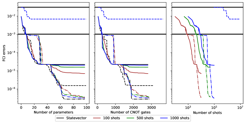
Figure 2: Convergence of adapt (dashed), enlm (full) and dsgn (dotted) with respect to the number of parameters (left), CNOT gates (middle) and the total number of shots (right) at a given precision of the obtained wave function for a linear $LiH$ molecule with 1.5 Angstrom separation between the atoms. The numbers for the finite shot simulations for adapt are not shown as the energy remained on the hf level.

In this section, the results from the setup described in Sec. IV are presented. We will conclude this section with a discussion of the results.

V.1 H4

In Fig. 1, we present the ground state calculations using adapt and algo with both importance metrics, enlm and dsgn, for a linear chain of $\text{H}_{4}$ in terms of the error relative to the FCI ground state energy. To an error of above $10^{-3}$ Hartree with respect to FCI, the convergence in terms of the number of operators (parameters) added to the Ansatz is very similar for all methods and numbers of shots per operator evaluation. Beyond that point, the fastest convergence is observed for the state vector simulation for adapt closely followed by the state vector for enlm and dsgn and finite shot simulations for dsgn. enlm converges slower for finite shot simulations. The slowest convergence with the number of operators added is observed for finite shot simulations for adapt. While dsgn calculations with a finite amount of shots are converged with about 25 parameters to an error of $10^{-9}$ Hartree, the precision for finite shot calculations using adapt is orders of magnitudes lower, at about $10^{-3}$ Hartree at the same point.

With respect to the resulting Ansatz depth, we observe that Ansätze constructed with the order of operators resulting from state vector simulations using the adapt metric result in the most compact circuits, followed by dsgn and enlm. Ansätze constructed with finite shot simulations for adapt are the least compact.

The total amount of shots for adapt and algo are very different. Both enlm and dsgn converge with a total number of shots about two orders of magnitude lower than the number of shots required for finite shot simulations using adapt. dsgn requires fewer shots to obtain a given precision compared to enlm.

V.2 LiH

Similar observations as for $\text{H}_{4}$ also hold true for the LiH calculations presented in Fig. 2, even though the overall convergence is slower. There are some other features to be observed in the convergence for this system. For example, the finite shot simulations for adapt with 100 and 500 shots per operator evaluation showed no sign of convergence and remained on the level of the hf reference state. The finite shot simulation with 1000 shots per operator evaluation shows early signs of convergence but is not able to go much below an energy difference of $10^{-2}$ Hartree. The adapt state vector simulation, and all simulations for dsgn and enlm converge to an energy difference of $10^{-3}$ Hartree at roughly the same rate, here the dsgn convergence flattens out, while the remaining calculations continue to converge at a similar rate. Beyond the addition of roughly 30 parameters dsgn gets a dramatic increase in precision while the other calculations start flattening out, displaying an unintuitive and seemingly erratic behaviour of convergence. It is notable that dsgn converges below the adapt state vector simulation.

With respect to Ansatz compactness and the number of shots required, similar conclusions hold true, displaying the same overall tendencies as observed for $\text{H}_{4}$ including the specific features described for the energy evaluation above.

V.3 Discussion

The dramatic difference in the number of shots between algo and adapt is due to the excessive amount of shots necessary to measure the gradients of the operator pool, $\mathcal{A}$, of adapt. We can write the total amount of shots as iterations times shots for algo whereas for adapt it reads iterations times shots times $|\mathcal{A}|$. Such a fact also provides another reason for the slow convergence of adapt when using a finite amount of shots as the evaluation of the gradient in Eq. (3) is prone to sampling error. In contrast, Eqns. (12) and (11) for enlm and dsgn are evaluated on a classical computer from states that are generated by the measurement of the energy. However, it remains be noticed that sampling error also effects enlm and dsgn as these methods are dependent on a representation of the weights of the determinants in the current wave function $|\Psi^{(k)}\rangle$. For adapt, more precise measurements of the gradients are required in order to improve convergence, while more precise sampling of the Slater determinants (diagonal elements of the Hamiltonian) becomes necessary for algo. This is especially important when the electronic structure becomes more correlated, i.e., when many determinants are required to describe the chemical system accurately, the necessary sampling depth may become a challenge.

It must also be noted that none of the proposed metrics for selecting the next operator is optimal and that there is room for improvement. For example, despite being the overall most competitive metric, dsgn seems to select some sub-optimal operators for LiH below $10^{-3}$ Hartree, yet it converges at an order of magnitude below the error which the adapt state vector simulation achieves beyond 60 parameters and enlm, which do not exhibit the same behaviour. Additionally, for LiH with the enlm metric the finite shot simulations with fewer shots achieve higher precisions indicating that this metric does not capture some important correlations in this particular system.

The results shown here suggest that for practical purposes the introduced heuristic metrics are good enough, since they converge at a similar rate as the adapt state vector simulations using a finite amount of shots. However, the systems shown here are rather small and the basis sets are limited. With the two different systems investigated, we have observed quite different detailed behaviours of convergence with no clear indication for why the ordering behaves so differently with different metrics. A better theoretical understanding of the limits of this method and a more rigorous derivation of metrics could make the convergence more robust across many systems and ensure that a similar convergence rate is retained for more complicated molecules and larger basis sets.

VI Conclusion

In this work, we have presented algo, a method for selecting operators based on the populations of Slater determinants in the wave function. We have introduced two different importance metrics dsgn and enlm and compared them to adapt in terms of the convergence to the FCI ground state energy. As was demonstrated, algo mitigates the significant measurement overhead for adapt by utilizing information about the population of Slater determinants in the wave function whereas adapt must evaluate the expectation value of gradient operators. For infinite shots, adapt provides the most compact wavefunction in terms of CNOT gates but with equal amount of parameters compared to algo. For finite shot simulations, algo yields more compact wave functions with dramatically reduced execution times. Of the two introduced importance metrics dsgn converged most rapidly and resulted in more compact circuits compared to enlm. However, we expect that a more systematic construction of importance metrics may improve the performance and eliminate some erratic features seen, e.g., for LiH. It remains to be seen how this method performs on real quantum hardware and in combination with other operator pools and other improvements available for adapt. This will be the topic of future investigations.

Conflicts of interest

NTZ is a co-founder of Kvantify Aps. The authors have filed a provisional patent application covering the method described here.

References

- [1] V. E. Elfving, B. W. Broer, M. Webber, J. Gavartin, M. D. Halls, K. P. Lorton, and A. Bochevarov, “How will quantum computers provide an industrially relevant computational advantage in quantum chemistry?,” Sept. 2020. arXiv:2009.12472 [physics, physics:quant-ph].
- [2] A. J. Daley, I. Bloch, C. Kokail, S. Flannigan, N. Pearson, M. Troyer, and P. Zoller, “Practical quantum advantage in quantum simulation,” Nature, vol. 607, pp. 667–676, July 2022. Number: 7920 Publisher: Nature Publishing Group.
- [3] J. F. Gonthier, M. D. Radin, C. Buda, E. J. Doskocil, C. M. Abuan, and J. Romero, “Identifying challenges towards practical quantum advantage through resource estimation: the measurement roadblock in the variational quantum eigensolver,” Tech. Rep. arXiv:2012.04001, arXiv, Dec. 2020. arXiv:2012.04001 [quant-ph] type: article.
- [4] A. Aspuru-Guzik, A. D. Dutoi, P. J. Love, and M. Head-Gordon, “Simulated quantum computation of molecular energies,” Science (New York, N.Y.), vol. 309, pp. 1704–1707, Sept. 2005.
- [5] K. Bharti, A. Cervera-Lierta, T. H. Kyaw, T. Haug, S. Alperin-Lea, A. Anand, M. Degroote, H. Heimonen, J. S. Kottmann, T. Menke, W.-K. Mok, S. Sim, L.-C. Kwek, and A. Aspuru-Guzik, “Noisy intermediate-scale quantum (NISQ) algorithms,” Reviews of Modern Physics, vol. 94, p. 015004, Feb. 2022. arXiv:2101.08448 [cond-mat, physics:quant-ph].
- [6] D. S. Abrams and S. Lloyd, “Quantum Algorithm Providing Exponential Speed Increase for Finding Eigenvalues and Eigenvectors,” Physical Review Letters, vol. 83, pp. 5162–5165, Dec. 1999. Publisher: American Physical Society.
- [7] J. R. McClean, J. Romero, R. Babbush, and A. Aspuru-Guzik, “The theory of variational hybrid quantum-classical algorithms,” New Journal of Physics, vol. 18, p. 023023, Feb. 2016. Publisher: IOP Publishing.
- [8] A. Kandala, A. Mezzacapo, K. Temme, M. Takita, M. Brink, J. M. Chow, and J. M. Gambetta, “Hardware-efficient Variational Quantum Eigensolver for Small Molecules and Quantum Magnets,” Nature, vol. 549, pp. 242–246, Sept. 2017. arXiv:1704.05018 [cond-mat, physics:quant-ph].
- [9] H. R. Grimsley, S. E. Economou, E. Barnes, and N. J. Mayhall, “An adaptive variational algorithm for exact molecular simulations on a quantum computer,” Nature Communications, vol. 10, p. 3007, July 2019. Number: 1 Publisher: Nature Publishing Group.
- [10] H. L. Tang, V. Shkolnikov, G. S. Barron, H. R. Grimsley, N. J. Mayhall, E. Barnes, and S. E. Economou, “Qubit-ADAPT-VQE: An Adaptive Algorithm for Constructing Hardware-Efficient Ans\”atze on a Quantum Processor,” PRX Quantum, vol. 2, p. 020310, Apr. 2021. Publisher: American Physical Society.
- [11] Y. S. Yordanov, V. Armaos, C. H. W. Barnes, and D. R. M. Arvidsson-Shukur, “Qubit-excitation-based adaptive variational quantum eigensolver,” Communications Physics, vol. 4, pp. 1–11, Oct. 2021. Number: 1 Publisher: Nature Publishing Group.
- [12] Z. Lan and W. Liang, “Amplitude Reordering Accelerates the Adaptive Variational Quantum Eigensolver Algorithms,” Journal of Chemical Theory and Computation, vol. 18, pp. 5267–5275, Sept. 2022. Publisher: American Chemical Society.
- [13] P. G. Anastasiou, Y. Chen, N. J. Mayhall, E. Barnes, and S. E. Economou, “TETRIS-ADAPT-VQE: An adaptive algorithm that yields shallower, denser circuit ans\”atze,” Sept. 2022. arXiv:2209.10562 [quant-ph].
- [14] L. W. Bertels, H. R. Grimsley, S. E. Economou, E. Barnes, and N. J. Mayhall, “Symmetry breaking slows convergence of the ADAPT Variational Quantum Eigensolver,” July 2022. arXiv:2207.03063 [quant-ph].
- [15] I. G. Ryabinkin, T.-C. Yen, S. N. Genin, and A. F. Izmaylov, “Qubit Coupled Cluster Method: A Systematic Approach to Quantum Chemistry on a Quantum Computer,” Journal of Chemical Theory and Computation, vol. 14, pp. 6317–6326, Dec. 2018. Publisher: American Chemical Society.
- [16] I. G. Ryabinkin, R. A. Lang, S. N. Genin, and A. F. Izmaylov, “Iterative Qubit Coupled Cluster approach with efficient screening of generators,” Tech. Rep. arXiv:1906.11192, arXiv, Oct. 2019. arXiv:1906.11192 [physics, physics:quant-ph] type: article.
- [17] J. Romero, R. Babbush, J. R. McClean, C. Hempel, P. Love, and A. Aspuru-Guzik, “Strategies for quantum computing molecular energies using the unitary coupled cluster ansatz,” Feb. 2018. arXiv:1701.02691 [quant-ph].
- [18] A. Anand, P. Schleich, S. Alperin-Lea, P. W. K. Jensen, S. Sim, M. Díaz-Tinoco, J. S. Kottmann, M. Degroote, A. F. Izmaylov, and A. Aspuru-Guzik, “A Quantum Computing View on Unitary Coupled Cluster Theory,” Chemical Society Reviews, vol. 51, no. 5, pp. 1659–1684, 2022. arXiv:2109.15176 [physics, physics:quant-ph].
- [19] J. Lee, W. J. Huggins, M. Head-Gordon, and K. B. Whaley, “Generalized Unitary Coupled Cluster Wave functions for Quantum Computation,” Journal of Chemical Theory and Computation, vol. 15, pp. 311–324, Jan. 2019. Publisher: American Chemical Society.
- [20] B. Huron, J. P. Malrieu, and P. Rancurel, “Iterative perturbation calculations of ground and excited state energies from multiconfigurational zeroth‐order wavefunctions,” The Journal of Chemical Physics, vol. 58, pp. 5745–5759, June 1973. Publisher: American Institute of Physics.
- [21] L. Bytautas and K. Ruedenberg, “A priori identification of configurational deadwood,” Chemical Physics, vol. 356, pp. 64–75, Feb. 2009.
- [22] J. S. M. Anderson, F. Heidar-Zadeh, and P. W. Ayers, “Breaking the curse of dimension for the electronic Schrödinger equation with functional analysis,” Computational and Theoretical Chemistry, vol. 1142, pp. 66–77, Oct. 2018.
- [23] C. F. Bender and E. R. Davidson, “Studies in Configuration Interaction: The First-Row Diatomic Hydrides,” Physical Review, vol. 183, pp. 23–30, July 1969. Publisher: American Physical Society.
- [24] J. L. Whitten and M. Hackmeyer, “Configuration Interaction Studies of Ground and Excited States of Polyatomic Molecules. I. The CI Formulation and Studies of Formaldehyde,” The Journal of Chemical Physics, vol. 51, pp. 5584–5596, Dec. 1969. Publisher: American Institute of Physics.
- [25] S. Evangelisti, J.-P. Daudey, and J.-P. Malrieu, “Convergence of an improved CIPSI algorithm,” Chemical Physics, vol. 75, pp. 91–102, Feb. 1983.
- [26] P. S. Epstein, “The Stark Effect from the Point of View of Schroedinger’s Quantum Theory,” Physical Review, vol. 28, pp. 695–710, Oct. 1926. Publisher: American Physical Society.
- [27] R. K. Nesbet and D. R. Hartree, “Configuration interaction in orbital theories,” Proceedings of the Royal Society of London. Series A. Mathematical and Physical Sciences, vol. 230, pp. 312–321, Jan. 1997. Publisher: Royal Society.
- [28] F. A. Evangelista, G. K.-L. Chan, and G. E. Scuseria, “Exact parameterization of fermionic wave functions via unitary coupled cluster theory,” The Journal of Chemical Physics, vol. 151, p. 244112, Dec. 2019. Publisher: American Institute of Physics.
- [29] P. Jordan and E. Wigner, “Über das Paulische Äquivalenzverbot,” Zeitschrift für Physik, vol. 47, pp. 631–651, Sept. 1928.
- [30] T. Tsuchimochi, M. Taii, T. Nishimaki, and S. L. Ten-no, “Adaptive construction of shallower quantum circuits with quantum spin projection for fermionic systems,” Physical Review Research, vol. 4, p. 033100, Aug. 2022.
- [31] A. tA v, M. S. ANIS, Abby-Mitchell, H. Abraham, AduOffei, R. Agarwal, G. Agliardi, M. Aharoni, V. Ajith, I. Y. Akhalwaya, G. Aleksandrowicz, T. Alexander, M. Amy, S. Anagolum, André, Anthony-Gandon, I. F. Araujo, E. Arbel, E. Arellano, A. Asfaw, I. E. Ashimine, A. Athalye, A. Avkhadiev, C. Azaustre, P. BHOLE, V. Bajpe, A. Banerjee, S. Banerjee, W. Bang, A. Bansal, P. Barkoutsos, A. Barnawal, G. Barron, G. S. Barron, L. Bello, Y. Ben-Haim, M. C. Bennett, D. Bevenius, D. Bhatnagar, P. Bhatnagar, A. Bhobe, P. Bianchini, L. S. Bishop, C. Blank, S. Bolos, S. Bopardikar, S. Bosch, S. Brandhofer, Brandon, S. Bravyi, Bryce-Fuller, D. Bucher, L. Burgholzer, A. Burov, F. Cabrera, P. Calpin, L. Capelluto, J. Carballo, G. Carrascal, A. Carriker, I. Carvalho, R. Chakrabarti, A. Chen, C.-F. Chen, E. Chen, J. C. Chen, R. Chen, F. Chevallier, K. Chinda, R. Cholarajan, J. M. Chow, S. Churchill, CisterMoke, C. Claus, C. Clauss, C. Clothier, R. Cocking, R. Cocuzzo, J. Connor, F. Correa, Z. Crockett, A. J. Cross, A. W. Cross, S. Cross, J. Cruz-Benito, C. Culver, A. D. Córcoles-Gonzales, N. D, S. Dague, T. E. Dandachi, A. N. Dangwal, J. Daniel, DanielAja, M. Daniels, M. Dartiailh, A. R. Davila, F. Debouni, A. Dekusar, A. Deshmukh, M. Deshpande, D. Ding, J. Doi, E. M. Dow, P. Downing, E. Drechsler, M. S. Drudis, E. Dumitrescu, K. Dumon, I. Duran, K. EL-Safty, E. Eastman, G. Eberle, A. Ebrahimi, P. Eendebak, D. Egger, EgrettaThula, ElePT, I. Elsayed, Emilio, A. Espiricueta, M. Everitt, D. Facoetti, Farida, P. M. Fernández, S. Ferracin, D. Ferrari, A. H. Ferrera, R. Fouilland, A. Frisch, A. Fuhrer, B. Fuller, M. GEORGE, J. Gacon, B. G. Gago, C. Gambella, J. M. Gambetta, A. Gammanpila, L. Garcia, T. Garg, S. Garion, J. R. Garrison, J. Garrison, T. Gates, N. Gavrielov, G. Gentinetta, H. Georgiev, L. Gil, A. Gilliam, A. Giridharan, Glen, J. Gomez-Mosquera, Gonzalo, S. de la Puente González, J. Gorzinski, I. Gould, D. Greenberg, D. Grinko, A. Großardt, W. Guan, D. Guijo, Guillermo-Mijares-Vilarino, J. A. Gunnels, H. Gupta, N. Gupta, J. M. Günther, M. Haglund, I. Haide, I. Hamamura, O. C. Hamido, F. Harkins, K. Hartman, A. Hasan, V. Havlicek, J. Hellmers, Ł. Herok, R. Hill, S. Hillmich, I. Hincks, C. Hong, H. Horii, C. Howington, S. Hu, W. Hu, C.-H. Huang, J. Huang, R. Huisman, H. Imai, T. Imamichi, K. Ishizaki, Ishwor, R. Iten, T. Itoko, A. Ivrii, A. Jalali, A. Javadi, A. Javadi-Abhari, W. Javed, Q. Jianhua, M. Jivrajani, K. Johns, S. Johnstun, Jonathan-Shoemaker, JosDenmark, JoshDumo, J. Judge, T. Kachmann, A. Kale, N. Kanazawa, J. Kane, Kang-Bae, A. Kapila, A. Karazeev, P. Kassebaum, T. Kato, T. Kehrer, J. Kelso, S. Kelso, H. van Kemenade, V. Khanderao, S. King, Y. Kobayashi, Kovi11Day, A. Kovyrshin, J. Krishna, R. Krishnakumar, P. Krishnamurthy, V. Krishnan, K. Krsulich, P. Kumkar, G. Kus, LNoorl, R. LaRose, E. Lacal, R. Lambert, H. Landa, J. Lapeyre, D. Lasecki, J. Latone, S. Lawrence, C. Lee, G. Li, T. J. Liang, J. Lishman, D. Liu, P. Liu, Lolcroc, A. K. M, L. Madden, Y. Maeng, S. Maheshkar, K. Majmudar, A. Malyshev, M. E. Mandouh, J. Manela, Manjula, J. Marecek, M. Marques, K. Marwaha, D. Maslov, P. Maszota, D. Mathews, A. Matsuo, F. Mazhandu, D. McClure, M. McElaney, J. McElroy, C. McGarry, D. McKay, D. McPherson, S. Meesala, D. Meirom, C. Mendell, T. Metcalfe, M. Mevissen, A. Meyer, A. Mezzacapo, R. Midha, A. Miessen, D. Millar, D. Miller, H. Miller, Z. Minev, A. Mitchell, A. Mohammad, N. Moll, A. Montanez, G. Monteiro, M. D. Mooring, R. Morales, N. Moran, D. Morcuende, S. Mostafa, M. Motta, R. Moyard, P. Murali, D. Murata, J. Müggenburg, T. NEMOZ, D. Nadlinger, K. Nakanishi, G. Nannicini, P. Nation, E. Navarro, Y. Naveh, S. W. Neagle, P. Neuweiler, A. Ngoueya, T. Nguyen, J. Nicander, Nick-Singstock, P. Niroula, H. Norlen, NuoWenLei, L. J. O’Riordan, O. Ogunbayo, P. Ollitrault, T. Onodera, R. Otaolea, S. Oud, D. Padilha, H. Paik, S. Pal, Y. Pang, A. Panigrahi, V. R. Pascuzzi, S. Perriello, E. Peterson, A. Phan, K. Pilch, F. Piro, M. Pistoia, C. Piveteau, J. Plewa, P. Pocreau, C. Possel, A. Pozas-Kerstjens, R. Pracht, M. Prokop, V. Prutyanov, S. Puri, D. Puzzuoli, Pythonix, J. Pérez, Quant02, Quintiii, R. I. Rahman, A. Raja, R. Rajeev, I. Rajput, N. Ramagiri, A. Rao, R. Raymond, O. Reardon-Smith, R. M.-C. Redondo, M. Reuter, J. Rice, M. Riedemann, Rietesh, D. Risinger, P. Rivero, M. L. Rocca, D. M. Rodríguez, RohithKarur, B. Rosand, M. Rossmannek, M. Ryu, T. SAPV, N. R. C. Sa, A. Saha, A. Ash-Saki, A. Salman, S. Sanand, M. Sandberg, H. Sandesara, R. Sapra, H. Sargsyan, A. Sarkar, N. Sathaye, N. Savola, B. Schmitt, C. Schnabel, Z. Schoenfeld, T. L. Scholten, E. Schoute, J. Schuhmacher, M. Schulterbrandt, J. Schwarm, P. Schweigert, J. Seaward, Sergi, D. E. Serrano, I. F. Sertage, K. Setia, F. Shah, P. A. Shah, N. Shammah, W. Shanks, R. Sharma, P. Shaw, Y. Shi, J. Shoemaker, A. Silva, A. Simonetto, D. Singh, D. Singh, P. Singh, P. Singkanipa, Y. Siraichi, Siri, J. Sistos, J. Sistos, I. Sitdikov, S. Sivarajah, Slavikmew, M. B. Sletfjerding, J. A. Smolin, M. Soeken, I. O. Sokolov, I. Sokolov, V. P. Soloviev, SooluThomas, Starfish, D. Steenken, M. Stypulkoski, A. Suau, S. Sun, K. J. Sung, M. Suwama, O. Słowik, R. Taeja, H. Takahashi, T. Takawale, I. Tavernelli, C. Taylor, P. Taylour, S. Thomas, K. Tian, M. Tillet, M. Tod, M. Tomasik, C. Tornow, E. de la Torre, J. L. S. Toural, K. Trabing, M. Treinish, D. Trenev, TrishaPe, F. Truger, TsafrirA, G. Tsilimigkounakis, K. Tsuoka, D. Tulsi, D. Tuna, W. Turner, K. Ueda, Y. Vaknin, C. R. Valcarce, F. Varchon, A. Vartak, A. C. Vazquez, P. Vijaywargiya, V. Villar, B. Vishnu, D. Vogt-Lee, C. Vuillot, WQ, J. Weaver, J. Weidenfeller, R. Wieczorek, J. A. Wildstrom, J. Wilson, E. Winston, WinterSoldier, J. J. Woehr, S. Woerner, R. Woo, C. J. Wood, R. Wood, S. Wood, J. Wootton, M. Wright, L. Xing, J. YU, Yaiza, B. Yang, U. Yang, J. Yao, D. Yeralin, R. Yonekura, D. Yonge-Mallo, R. Yoshida, R. Young, J. Yu, L. Yu, Yuma-Nakamura, C. Zachow, L. Zdanski, H. Zhang, E. Zheltonozhskii, I. Zidaru, B. Zimmermann, B. Zindorf, C. Zoufal, a matsuo, aeddins ibm, alexzhang13, b63, bartek bartlomiej, bcamorrison, brandhsn, nick bronn, chetmurthy, choerst ibm, comet, dalin27, deeplokhande, dekel.meirom, derwind, dime10, ehchen, ewinston, fanizzamarco, fs1132429, gadial, galeinston, georgezhou20, georgios ts, gruu, hhorii, hhyap, hykavitha, itoko, jeppevinkel, jessica angel7, jezerjojo14, jliu45, johannesgreiner, jscott2, kUmezawa, klinvill, krutik2966, luciacuervovalor, ma5x, merav aharoni, michelle4654, msuwama, nico lgrs, nrhawkins, ntgiwsvp, ordmoj, sagar pahwa, pritamsinha2304, rickyzcode, rithikaadiga, ryancocuzzo, saktar unr, saswati qiskit, sebastian mair, septembrr, sethmerkel, sg495, shaashwat, smturro2, sternparky, strickroman, tigerjack, tsura crisaldo, upsideon, vadebayo49, welien, willhbang, wmurphy collabstar, yang.luh, yuri@FreeBSD, and M. Čepulkovskis, “Qiskit: An open-source framework for quantum computing,” 2021.