Fundamental speed limits on entanglement dynamics of bipartite quantum systems

Abstract

The speed limits on entanglement are defined as the maximal rate at which entanglement can be generated or degraded in a physical process. We derive the speed limits on entanglement, using the relative entropy of entanglement and trace-distance entanglement, for unitary as well as for arbitrary quantum dynamics, where we assume that the dynamics of the closest separable state can be approximately described by the closest separable dynamics of the actual dynamics of the system. For unitary dynamics of isolated bipartite systems which are described by pure states, the rate of entanglement production is bounded by the product of fluctuations of the system’s driving Hamiltonian and the surprisal operator, with an additional term reflecting the time-dependent nature of the closest separable state. Removing restrictions on the purity of the input and on the unitarity of the evolution, the two terms in the bound get suitably altered. Furthermore, we find a lower bound on the time required to generate or degrade a certain amount of entanglement by arbitrary quantum dynamics. We demonstrate the tightness of our speed limits on entanglement by considering quantum processes of practical interest.

I Introduction

Quantum speed limits (QSLs) are the fundamental limitations imposed by quantum mechanics on the rate at which quantum mechanical systems and their observables evolve in a physical process. Initially, QSLs were formulated for unitary dynamics of pure states Mandelstam and Tamm (1945); Margolus and Levitin (1998); Anandan and Aharonov (1990); Pati et al. (2023); Thakuria and Pati (2022). Later it was generalized for unitary dynamics of mixed states Uhlmann (1992), entangling dynamics Giovannetti et al. (2004); J and Hernández (2022); Krisnanda et al. (2022), dissipative quantum dynamics Shiraishi and Saito (2021); Funo et al. (2019); Van Vu and Saito (2023); Pires et al. (2016); Brody and Longstaff (2019); Taddei et al. (2013); del Campo et al. (2013); Campaioli et al. (2013); Deffner and Lutz (2013); Kiselev et al. (2022), and arbitrary dynamics Thakuria et al. (2022). The QSLs are essential for the theoretical understanding of quantum dynamics and have substantial practical relevance in developing quantum technologies. QSLs have several applications in various quantum technologies such quantum computing Ashhab et al. (2012); Aifer and Deffner (2022), quantum metrology Campbell et al. (2018); Beau and del Campo (2017), optimal control theory Caneva et al. (2009); Deffner and Campbell (2017), quantum communication Murphy et al. (2010), quantum batteries Mohan and Pati (2021, 2022); Campaioli et al. (2017) and quantum refrigerator Mukhopadhyay et al. (2018).

Entanglement is one of the remarkable features of quantum theory with no counterpart in a classical theory Einstein et al. (1935); Bell (1964). It is a feature of composite systems which implies that there exists a set of global states such that any element of this set can not be written as a mixture of products of states of the individual subsystems. In 1964 John Bell derived an inequality for composite systems assuming that the physical world is described by a local hidden variable model and showed that certain entangled states can violate this inequality Bell (1964). From this perspective, entanglement can be seen as a characteristic feature of quantum theory and is impossible to generically simulate in any classical formalism. Entanglement is a key resource for several information processing tasks such as quantum teleportation Bennett et al. (1993), quantum dense coding Bennett and Wiesner (1992), quantum cryptography Ekert (1991), quantum communication Bennett and Wiesner (1992), quantum computation Jozsa (1997); Jozsa and Linden (2003), quantum random number generators Colbeck and Renner (2012), quantum metrology Dowling (2008), etc. Therefore, understanding the dynamics of entanglement, we can uncover new ways to generate and manipulate it for a variety of applications. Additionally, studying the dynamics of entanglement helps us gain insight into the behaviour of quantum systems. There has been a significant amount of interest in studying entanglement dynamics in various physical systems, including many-body and optomechanical systems Ho and Abanin (2017); Elsayed et al. (2018); Brandão et al. (2020).

Quantum speed limits on the time evolution of quantum systems were traditionally derived based on the distinguishability of the two quantum states: the initial and final states. Recently, some other formulations of QSLs have been studied, which focused on the rate of change of different quantities, such as the expectation value of observables Mohan and Pati (2022); Gong and Hamazaki (2022); Hamazaki (2023); García-Pintos et al. (2022); Hamazaki (2022), auto-correlation function Hörnedal et al. (2023); Carabba et al. (2022); Hasegawa (2023), quantumness Jing et al. (2016), quantum coherence Mohan et al. (2022), entanglement Bera et al. (2013); Rudnicki (2021); Pandey et al. (2023); Shrimali et al. (2022), quantum resources Campaioli et al. (2022), information measures Mohan et al. (2022); Pires (2022); Pires et al. (2021), and correlations Pandey et al. (2023); Paulson and Banerjee (2022).

Entanglement is an invaluable resource in quantum information and computation. However, it is a seemingly fragile quantum resource and can easily be degraded by undesirable but practically unavoidable interactions with the environment, such as decoherence and dissipation. An area of ongoing research is to understand and control the dynamics of entanglement between two subsystems by tuning their interaction in the presence of noise Shaham et al. ; Nosrati et al. (2020); Schachenmayer et al. (2013). Similarly, there is a need for further work to speed up the generation of entanglement in various quantum systems that are commonly used in quantum technologies using quantum control methods. Consequently, the study of quantum speed limits on entanglement generation, manipulation and degradation is of critical significance.

The speed limits on entanglement dynamics answer the fundamental question, “how fast can entanglement be generated or degraded in a physical process?” The speed limits on entanglement dynamics are typically obtained as upper bounds on the rate of change of entanglement of a quantum system in a physical process. Thus, they also provide the lower bounds on the time required to change the entanglement of a quantum system by a certain amount. Traditionally, the speed limits on entanglement dynamics were studied for unitary dynamics of quantum systems using suitable entanglement measures such as entanglement entropy Shrimali et al. (2022); Hamilton and Clark (2023); Pandey et al. (2023), concurrence Pandey et al. (2023), and geometric measure of entanglement Bera et al. (2013); Rudnicki (2021). Recently, speed limits on entanglement have been generalized to arbitrary dynamics using entanglement measures such as negativity Pandey et al. (2023). Negativity, however, cannot quantify the entanglement of bound-entangled statesHorodecki et al. (1998). It is therefore interesting to derive the speed limits on entanglement using a suitable entanglement measure that does not have such shortcomings. In Ref. Campaioli et al. (2022), a resource speed limit is introduced, which describes how fast quantum resources can be generated or degraded by physical processes. The resource speed limit is derived from a relative entropy-based measure, which also applies to entanglement. In general, when the state of the given system changes in time, the free state which minimizes the relative entropy also changes at each instant of time. In Ref. Campaioli et al. (2022), while deriving the resource speed limit, the authors considered the free state as fixed (stationary) for simplicity. Therefore, the bounds presented in Ref.  Campaioli et al. (2022), while very important and general, can potentially be loose.

In the context of the relative entropy of entanglementVedral et al. (1997), the free states are separable states. We focus on the dynamics of the closest separable state which minimizes the relative entropy of entanglement at each instant of time when the state of a given quantum system evolves in time. Any map which describes the dynamics of the closest separable state is potentially one that maps separable states to separable states. In other words, the dynamics of the closest separable state is considered to be an entanglement non-generating map for separable initial states. This can in principle, be a LOCC map or a separable map. In this paper, we first assume that the dynamics of the closest separable state can be modelled by the nearest separable map of the given dynamics, which governs the evolution of the given bipartite system. Further in this paper, we derive speed limits on the entanglement of a bipartite system evolving under arbitrary dynamical processes. To obtain the speed limits on entanglement, we use the relative entropy of entanglement Vedral et al. (1997) and the trace distance of entanglement Eisert et al. (2003) as entanglement measures. We have estimated speed limits on entanglement for some quantum processes of practical interest, such as unitary dynamics generated by a non-local Hamiltonian and pure dephasing dynamics.

The structure of this paper is as follows. In Section II, we present the preliminaries and background necessary to derive the main results of this paper. In Section III, we provide a method to determine the closest separable dynamics to a given dynamics. In Section IV, we derive the speed limits on entanglement for unitary and arbitrary CPTP dynamics using the relative entropy of entanglement and the trace distance of entanglement. In Section V, we discuss some examples to show the tightness of our speed limit bounds. Finally, in Section VI, we summarise our findings.

II Definitions and Preliminaries

Let $\mathcal{H}$ denote a separable Hilbert space with ${\mathrm{d}im}\left(\mathcal{H}\right)$ denoting the dimension of $\mathcal{H}$. A linear map $T:{\mathcal{H}\rightarrow\mathcal{H}}$ is called a bounded linear operator if there exists a constant $\alpha\in[0,\infty)$ such that $\|T\ket{\psi}\|\leq\alpha\|\ket{\psi}\|$ for all $\ket{\psi}\in\mathcal{H}$, where $\|\ket{\psi}\|=\sqrt{\innerproduct{\psi}{\psi}}$. Let $\mathcal{L}(\mathcal{H})$ denotes the set of all bounded linear operators acting on $\mathcal{H}$, with $\mathcal{I}_{\mathcal{H}}$ denoting the identity operator. The subset of $\mathcal{L}(\mathcal{H})$, containing all positive semi-definite operators is denoted by $\mathcal{L}(\mathcal{H})_{+}$. An operator $\mathcal{O}\in\mathcal{L}(\mathcal{H})$ is called trace-class if $\operatorname{tr}(\left|{\mathcal{O}}\right|)=\sum_{i}\left<i\left|{\mathcal{O}}\right|,i\right>$, where $\{\ket{i}\}^{\infty}_{i=1}$ is an orthonormal basis in $\mathcal{H}$ and $\left|{\mathcal{O}}\right|=\sqrt{{\mathcal{O}}^{\dagger}{\mathcal{O}}}$, is finite, i.e., $\operatorname{tr}({\left|{\mathcal{O}}\right|})<\infty$. Let ${\mathcal{L}}^{\prime}(\mathcal{H})_{+}$ denote the subset of $\mathcal{L}(\mathcal{H})$ containing all positive semi-definite, trace class operators acting on $\mathcal{H}$. The state of a quantum system, denoted by $\rho$, is an element of ${\mathcal{L}^{\prime}(\mathcal{H}})_{+}$ with unit trace and is called a density operator. We denote with ${\mathcal{S}(\mathcal{H})}$, the set of density operators acting on the Hilbert space $\mathcal{H}$. Let $\mathcal{H}_{A}$ denote the Hilbert space associated with a quantum system $A$. States of the system $A$ are represented by density operators $\rho_{A}\in{\mathcal{S}(\mathcal{H}_{A})}$. For a composite system $AB$, the combined Hilbert space is the tensor product $\mathcal{H}_{AB}:=\mathcal{H}_{A}\otimes\mathcal{H}_{B}$ of the individual Hilbert spaces. A state of the composite system $AB$ is represented by a density operator $\rho_{AB}\in\mathcal{S}(\mathcal{H}_{AB})$, and the reduced density operator of the subsystem $A$ (or $B$) is obtained by applying the partial trace operation $\operatorname{tr}_{B}$ (or $\operatorname{tr}_{A}$) over the combined density operator $\rho_{AB}$, i.e., $\rho_{A}=\operatorname{tr}_{B}(\rho_{AB})$, and similarly for $B$. A quantum system is said to be in a pure state when there is no uncertainty in the knowledge of its state. The density operator representing a pure state $\Psi\in\mathcal{S}(\mathcal{H})$ is a rank-one projection operator i.e. $\Psi=\outerproduct{\Psi}{\Psi}$ (an idempotent matrix, i.e., $\Psi^{2}=\Psi$), where $\ket{\Psi}\in\mathcal{H}$. Otherwise, $\rho$ is in a mixed state and can be written as a convex mixture of pure states $\Psi_{i}$ with mixing probabilities $p_{i}$, i.e., $\rho=\sum_{i}p_{i}\Psi_{i}$. In this paper, we will denote pure states with $\Psi$.

The Schatten-p norm of an operator ${\mathcal{O}}\in\mathcal{L}(\mathcal{H})$ is defined as

$$\norm{{\mathcal{O}}}_{p}=\left(\operatorname{tr}\left|{\mathcal{O}}\right|^{p}\right)^{1/p},$$ (1)

where $\left|{\mathcal{O}}\right|=\sqrt{{\mathcal{O}}^{\dagger}{\mathcal{O}}}$, $p\geq 1,\ p\in\mathbb{R}$. The operator norm, the Hilbert-Schmidt norm, and the trace norm correspond to $p=\infty,2,1$ respectively and satisfy the inequality $\norm{A}_{\mathrm{\infty}}\leq\norm{A}_{\mathrm{2}}\leq\norm{A}_{\mathrm{1}}$.

Uncertainty relation for mixed states.– For any two observables $\{{\mathcal{O}}_{1}$, ${\mathcal{O}}_{2}\}\in{\mathcal{L}}(\mathcal{H})$, and $\rho\in{\mathcal{S}}(\mathcal{H})$, the following inequality holds Luo (2005)

$$\frac{1}{4}\left|\operatorname{tr}\left([{\mathcal{O}}_{1},{\mathcal{O}}_{2}]\rho\right)\right|^{2}\leq U_{{\mathcal{O}}_{1}}U_{{\mathcal{O}}_{2}},$$ (2)

where $U_{\mathcal{O}}=\sqrt{V^{2}_{\mathcal{O}}-(V_{\mathcal{O}}-I_{\mathcal{O}})^{2}}$ for an operator ${\mathcal{O}}\in{\mathcal{L}}(\mathcal{H})$, $V_{\mathcal{Q}}=\operatorname{tr}(\rho{\mathcal{O}}^{2})-(\operatorname{tr}(\rho{\mathcal{O}}))^{2}$ is variance of the operator $\mathcal{O}$ in the state $\rho$, and $I_{\mathcal{O}}$ is Wigner-Yanase skew information, defined as :

$$I_{\mathcal{Q}}=-\frac{1}{2}\operatorname{tr}\left([\sqrt{\rho},{\mathcal{O}}]^{2}\right).$$ (3)

One can easily check that the above uncertainty reduces to well known Robertson uncertainty relation Robertson (1929), when $\rho$ is a pure state.

Quantum dynamics.– For any dynamical quantum system with associated Hilbert space $\mathcal{H}$, the state of the system, generically, changes with time. The time evolution of the state of the system is given by a dynamical map which maps an initial state to a final state and it should satisfy the following properties:
$(i)$ Linearity.– A map $\mathcal{M}:\mathcal{L}({\mathcal{H}}_{A})\rightarrow\mathcal{L}({\mathcal{H}}_{B})$ is called linear if ${\mathcal{M}}(aX_{A}+bY_{A})=a\Phi(X_{A})+b\Phi(Y_{A})$, where $X_{A},Y_{A}\in{\mathcal{L}(\mathcal{H}}_{A})$ and $a,b\in\mathbb{C}$. $(ii)$ Complete Positivity .– A linear map $\mathcal{M}:\mathcal{L}({\mathcal{H}}_{A})\rightarrow\mathcal{L}({\mathcal{H}}_{B})$ is called positive if $\mathcal{M}\left(\eta_{A}\right)\in\mathcal{L}({\mathcal{H}}_{B})_{+}~{}\forall~{}\eta_{A}~{}\in\mathcal{L}({\mathcal{H}}_{A})_{+}$ and completely positive if $\mathrm{i}d_{R}\otimes\mathcal{M}$ (where $\mathrm{i}d_{R}$ denotes the identity super-operator acting on an arbitrary reference system $R$) is also a positive map. $(iii)$ Preservation of Trace.– A map $\mathcal{M}:\mathcal{L}({\mathcal{H}}_{A})_{+}\rightarrow\mathcal{L}({\mathcal{H}}_{B})_{+}$ is called trace preserving if $\operatorname{tr}\left(\mathcal{M}(\eta_{A})\right)=\operatorname{tr}(\eta_{A})~{}\forall~{}\eta_{A}\in{\mathcal{L}}({\mathcal{H}}_{A})$.

A mapping which fulfils the above three conditions is called a quantum channel (dynamical map) and it describes a physically meaningful evolution of density operators. Sometimes it could be easier to use differential equations to describe the evolution instead of quantum channels:

$$\dot{\rho_{t}}:=\diff{\rho_{t}}{t}=\mathcal{L}_{t}(\rho_{t}),$$ (4)

where $\mathcal{L}_{t}$ is the Liouvillian super-operator Rivas and Huelga (2012) which in general can be time independent or time-dependent.

CJ isomorphism.– Let $\mathcal{H}_{R}$ be a Hilbert space isomorphic to another Hilbert space $\mathcal{H}_{A}$ and let their orthonormal bases be $\{\ket{i}_{R}\}$ and $\{\ket{i}_{A}\}$ respectively. Now the space $\mathcal{L}(\mathcal{L}(\mathcal{H}_{A}),\mathcal{L}({\mathcal{H}}_{B}))$ of linear maps $\mathcal{E}:{\mathcal{L}(\mathcal{H}}_{A})\rightarrow\mathcal{L}({\mathcal{H}}_{B})$ and the tensor product space $\mathcal{L}(\mathcal{H}_{R})\otimes\mathcal{L}(\mathcal{H}_{B})$ are isomorphic under the following identification:

$$\mathcal{E}\leftrightarrow\Phi_{RB} \equiv({\mathrm{i}d}_{R}\otimes\mathcal{E})\left(\left(\outerproduct{\Psi}{\Psi})_{RA}\right)\right)$$

$$=\sum_{i,j}\outerproduct{i}{j}_{R}\otimes\mathcal{E}(\outerproduct{i}{j}_{A})$$ (5)

where $\ket{\Psi}=\sum_{i}\ket{i}_{R}\otimes\ket{i}_{A}$ is an unnormalized maximally entangled state of $RA$. The $\mathcal{E}\leftrightarrow\Phi_{RB}$ correspondence is known as the Choi-Jamiołkowski(CJ) isomorphism and the operator $\Phi_{RB}$ is known as the Choi operator of the linear map $\mathcal{E}$. Choi’s theorem for a completely positive map guarantees that $\Phi_{RB}$ is positive semi-definite if and only if $\mathcal{E}$ is completely positive. Similarly a CP map $\mathcal{M}_{AB}$ on a bipartite system $AB$ can have a Choi operator representation given by

$$\Phi_{AA^{\prime}BB^{\prime}}=({\mathrm{i}d}_{A^{\prime}B^{\prime}}\otimes\mathcal{M}_{AB})(\Psi_{AA^{\prime}}\otimes\Psi_{BB^{\prime}}),$$ (6)

where $\mathcal{H}_{A}^{\prime}$ and $\mathcal{H}_{B}^{\prime}$ are isomorphic to $\mathcal{H}_{A}$ and $\mathcal{H}_{B}$ respectively. $\Psi_{AA^{\prime}}$ and $\Psi_{BB^{\prime}}$ are the maximally entangled states on $\mathcal{H}_{AA^{\prime}}$ and $\mathcal{H}_{BB^{\prime}}$ respectively. Conversely, given a positive semi-definite operator on $AA^{\prime}BB^{\prime}$, the corresponding CP map is given by:

$$\mathcal{M}(\rho_{AB})=d^{2}\operatorname{tr}_{A^{\prime}B^{\prime}}(\Phi_{AA^{\prime}BB^{\prime}}\rho^{T}_{A^{\prime}B^{\prime}}\otimes\mathcal{I}_{AB})$$ (7)

where $T$ denotes transposition with respect to the chosen basis of $\mathcal{H}_{A^{\prime}}\otimes\mathcal{H}_{B^{\prime}}$ and we have taken the dimensions of all the systems to be $d$. Using the above relations, it can be shown that Cirac et al. (2001):

• $\mathcal{M}$ is separable iff $\Phi_{AA^{\prime}BB^{\prime}}$ is separable with respect to the systems $\mathcal{H}_{AA^{\prime}}$ and $\mathcal{H}_{BB^{\prime}}$.

• $\mathcal{M}$ can create entanglement iff $\Phi_{AA^{\prime}BB^{\prime}}$ is non separable with respect to the subsystems $\mathcal{H}_{AA^{\prime}}$ and $\mathcal{H}_{BB^{\prime}}$.

• If $\mathcal{M}$ corresponds to a unitary channel, then its Choi operator has rank one, i.e., it can be written as a projector: $\Phi_{AA^{\prime}BB^{\prime}}=\outerproduct{\phi}{\phi}$, where $\ket{\phi}$ is a state in $\mathcal{H}_{AA^{\prime}}\otimes\mathcal{H}_{BB^{\prime}}$.

von Neumann entropy.–The von Neumann entropy of a quantum state $\rho_{A}\in\mathcal{S}(\mathcal{H}_{A})$ is a non-negative quantity given by:

$$S(A)_{\rho}:=S(\rho_{A})=-\operatorname{tr}({\rho_{A}\log{\rho_{A}}}),$$ (8)

where the logarithm is taken to base 2. $S(\rho_{A})$ is manifestly invariant under a unitary transformation $\rho_{A}\rightarrow U\rho_{A}U^{{\dagger}}$, i.e., $S(\rho_{A})=S(U\rho_{A}U^{{\dagger}})$.

Relative entropy.– The quantum relative entropy between density operators $\rho\in\mathcal{S}(\mathcal{H})$ and a positive semi-definite operator $\sigma\in\mathcal{L}(\mathcal{H})$ is defined as follows Umegaki (1962)

$$D(\rho\|\sigma):=\begin{cases}\operatorname{tr}(\rho(\log{\rho}-\log{\sigma}))&\text{if}\ \operatorname{supp}(\rho)\subseteq\operatorname{supp}(\sigma),\\ +\infty&\text{otherwise},\end{cases}$$ (9)

where $\operatorname{supp}(\rho)$ and $\operatorname{supp}(\sigma)$ are the supports of $\rho$ and $\sigma$, respectively. The quantum relative entropy has a number of useful properties. $(i)$ $D(\rho\|\sigma)$ is invariant under unitary dynamics, i.e., $D(\rho\|\sigma)=D(U\rho U^{{\dagger}}\|U\sigma U^{{\dagger}})$, and non-increasing under the action of linear CPTP maps, i.e., $D(\rho\|\sigma)\geq D({\mathcal{N}}(\rho)\|{\mathcal{N}}(\sigma))$ for any density operators $\rho$ and $\sigma$ and for any linear CPTP map $\mathcal{N}$. $(ii)$ Relative entropy between two positive semi-definite operators $\rho$ and $\sigma$ is positive if $\rho\in\mathcal{S}(\mathcal{H})$, $\sigma\in{\mathcal{L}}^{\prime}(\mathcal{H})_{+}$ and $\operatorname{tr}(\sigma)\leq 1$, with equality if and only if $\sigma=\rho$. So, quantum relative entropy can also be thought as an appropriate measure of distinguishability or discrimination between $\rho$ and $\sigma$ which motivates one to think $D(\rho\|\sigma)$ as a kind of “metric” (a measure of distance) between density operators. Note that $D(\rho\|\sigma)$ is not a true metric because it is neither symmetric between $\rho$ and $\sigma$ nor it satisfies triangular inequality but it is an entropic measure of distance between two density matrices.

Separable states, separable operations and entanglement.– A bipartite quantum state $\sigma_{AB}$ is called separable (or completely disentangled) if it can be written or approximated in the following form Werner (1989):

$$\sigma_{AB}=\sum_{i}p_{i}\rho^{i}_{A}\otimes\rho^{i}_{B},$$ (10)

for some probability distribution $\{p_{i}\}_{i}$ and density operators $\rho^{i}_{A}$ and $\rho^{i}_{B}$. When subsystems $A$ and $B$ are finite-dimensional, we can choose $\rho^{i}_{A}$ and $\rho^{i}_{B}$ to be pure states. We let $\operatorname{SEP}(A;B)$ denote the set of separable states defined on $\mathcal{H}_{AB}$. An operation is called “separable operation” if its Kraus representation is given by:

$$\Lambda_{S}(\rho)=\sum_{i}A_{i}\otimes B_{i}\rho A_{i}^{\dagger}\otimes B^{\dagger}_{i},$$ (11)

which satisfy $\sum_{i}A_{i}A^{{\dagger}}_{i}\otimes B_{i}B^{{\dagger}}_{i}=\mathcal{I}\otimes\mathcal{I}$.

If $\sigma_{AB}$ is not separable then it is “entangled”. Entanglement works as a valuable resource for many quantum information processing tasks such as quantum teleportation, quantum metrology, quantum communication, quantum sensing, quantum random number generators, etc. So, it is desirable to have a measure that quantifies the amount of entanglement present in a state. There are several measures of entanglement which have been proposed namely entanglement entropy Bennett et al. (1996), concurrence Wootters (2001, 1998), negativity Vidal and Werner (2002), relative entropy of entanglement Vedral et al. (1997), trace distance of entanglement Eisert et al. (2003), etc. In this paper, we will consider the relative entropy of entanglement and trace distance of entanglement as measures of entanglement.

Relative entropy of entanglement.– The relative entropy of entanglement (REE) is an entanglement measure to quantify the amount of entanglement present in an arbitrary bipartite quantum state. It is a distance-based measure defined on the intuition that if a given state is geometrically close to the set of separable states it has less entanglement. For an arbitrary bipartite quantum state $\rho_{AB}\in{\mathcal{S}}({\mathcal{H}}_{AB})$, its relative entropy of entanglement is defined as Vedral et al. (1997)

$$E(\rho_{AB}):=\min_{\sigma\in\operatorname{SEP}(A;B)}D\left(\rho_{AB}\|\sigma_{AB}\right),$$ (12)

where each of $\dim(\mathcal{H}_{A})$ and $\dim(\mathcal{H}_{B})$ can be either finite or infinite. For a given quantum state $\rho_{AB}$, let us assume that minimization of the above equation is achieved for the separable state $\sigma^{*}_{AB}\in{\mathcal{S}}({\mathcal{H}}_{AB})$, i.e., $E(\rho_{AB})=D\left(\rho_{AB}\|\sigma^{*}_{AB}\right)$, which depends on the given state $\rho_{AB}$, i.e., $\sigma^{*}_{AB}=\sigma^{*}_{AB}(\rho_{AB})$. A separable state that realizes the minimum of Eq. (12) is called a closest separable state (CSS).

Trace Distance of entanglement.– Trace distance can also be used as a distance measure to define an entanglement monotone. For an arbitrary bipartite quantum state $\rho_{AB}\in{\mathcal{S}}({\mathcal{H}}_{AB})$, its trace distance of entanglement is defined as Eisert et al. (2003):

$$\mathcal{D}_{tr}(\rho_{AB})=\min_{\sigma\in\operatorname{SEP}(A;B)}\operatorname{tr}\left|\rho_{AB}-\sigma_{AB}\right|.$$ (13)

We have assumed that the dynamics of CSS can be approximated by the closest separable dynamics of a given dynamics. In the next section, we introduce a method to determine the closest separable dynamics of a given arbitrary CPTP dynamics. We first find the Choi dual of the given arbitrary CPTP map and then we use relative entropy to find its CSS. Using the Choi-Jmaiołkowski isomorphism we then find the CPTP map corresponding to the CSS. We call this CPTP map as the closest separable map for the given CPTP map. Then we study the dynamics of the CSS of a given state under the closest separable map obtained in this way.

III Dynamics of closest separable state

We start by finding the closest separable channel to a given channel by using Choi-Jamiołkowski isomorphism. For a given linear CP map $\mathcal{E}:{\mathcal{L}}^{\prime}({\mathcal{H}}_{AB})_{+}\rightarrow{\mathcal{L}}^{\prime}({\mathcal{H}}_{AB})_{+}$, the normalized CJ dual state is given by

$$\Phi_{AA^{\prime}BB^{\prime}}=\frac{1}{d^{2}}({\mathrm{i}d}_{A^{\prime}B^{\prime}}\otimes\mathcal{E}_{AB})(P_{AA^{\prime}}\otimes P_{BB^{\prime}}),$$ (14)

where $P_{AA^{\prime}}$ and $P_{BB^{\prime}}$ are maximally entangled states of $AA^{\prime}$ and $BB^{\prime}$ respectively, normalized to $\mathrm{min}\{\mathrm{dim(\mathcal{H}_{A})},\mathrm{dim(\mathcal{H}_{A^{\prime}})}\}$ and $\mathrm{min}\{\mathrm{dim(\mathcal{H}_{B})},\mathrm{dim(\mathcal{H}_{B^{\prime}})}\}$. We now find the closest separable state of this Choi operator using relative entropy as the distance measure, which is given as

$$\tilde{\Phi}=\operatorname*{Arg\,min}\{S(\Phi\|\chi):{\chi\in\operatorname{SEP}(AA^{\prime};BB^{\prime})}\}.$$ (15)

We define the closest separable map of given map $\mathcal{E}$ as the Choi dual of $\tilde{\Phi}$, given by

$$\mathcal{E}^{*}(\rho_{AB})=d^{2}\operatorname{tr}_{A^{\prime}B^{\prime}}(\tilde{\Phi}_{AA^{\prime}BB^{\prime}}\rho^{T}_{A^{\prime}B^{\prime}}\otimes\mathcal{I}_{AB}),$$ (16)

where $\mathcal{E}^{*}$ is the closest separable map of $\mathcal{E}$, its action on state $\rho_{AB}$ is given by the above equation, $\mathcal{I}_{AB}$ is identity operator on subsystem $AB$ and we have taken the dimension of all the systems to be $d$.

As an example now we will determine the closed separable map of unitary map. Let us consider a unitary map $\mathcal{E}$ represented by $U_{AB}={\mathrm{e}}^{-iH_{AB}t}$, where $H_{AB}$ is the Hamiltonian of $AB$, . In this case $\Phi$ is pure and an analytic expression of the closest separable state is known Vedral and Plenio (1998). For a given pure state in the Schmidt basis $\{\ket{\psi_{i}}\ket{\phi_{i}}\}$, and Schmidt coefficients $\sqrt{p_{i}}$, the density matrix is $\rho=\sum_{i,j}\sqrt{p_{i}p_{j}}\outerproduct{\psi_{i}\phi_{i}}{\psi_{j}\phi_{j}}$, and the closest separable state is

$$\rho^{*}=\sum_{i}p_{i}\outerproduct{\psi_{i}\phi_{i}}{\psi_{i}\phi_{i}}.$$ (17)

Let us choose the bases on the Hilbert spaces involved as follows:

$$\mathcal{H}_{A} =[\{\ket{\alpha_{i}}\}],\mathcal{H}_{A^{\prime}}=[\{\ket{\alpha^{\prime}_{j}}\}],$$

$$\mathcal{H}_{B} =[\{\ket{\beta_{m}}\}],\mathcal{H}_{B^{\prime}}=[\{\ket{\beta^{\prime}_{n}}\}].$$ (18)

Let the eigenstates of $H_{AB}$ be given by $\{\ket{e_{n}}_{AB}\}$ with the corresponding eigenvalues $\{E_{n}\}$. We also define the inner products between the energy eigenbasis and the product basis corresponding to the choice in the above equation as:

$$V^{k}_{ij}=\innerproduct{\alpha_{i}\beta_{j}}{e_{k}}_{AB}.$$ (19)

In terms of the above definitions, the Choi dual of $U_{AB}$ is a pure state in $\mathcal{H}_{AB}\otimes\mathcal{H}_{A^{\prime}B^{\prime}}$ and given by:

$$\Phi_{ABA^{\prime}B^{\prime}}=\sum_{i,j,m,n}R_{mi,nj}\ket{\alpha_{m}\alpha^{\prime}_{i}}_{AA^{\prime}}\ket{\beta_{n}\beta^{\prime}_{j}}_{BB^{\prime}},$$ (20)

where

$$R_{mi,nj}=\sum_{k}{V^{k}_{ij}}^{*}V^{k}_{mn}e^{-iE_{k}t}.$$ (21)

In order to find the closest separable state of $\Phi_{ABA^{\prime}B^{\prime}}$, we need to find the Schmidt decomposition of the state in Eq. (20) with respect to the bipartitions $AA^{\prime}:BB^{\prime}$. We need to choose a particular Hamiltonian for that. Then, the closest separable state is known in terms of the Schmidt basis of $\Phi_{ABA^{\prime}B^{\prime}}$. The Choi dual of the closest separable state of $\Phi_{ABA^{\prime}B^{\prime}}$ will give the closest separable operation.

In the case of mixed states or non-unitary evolution, finding the analytical expression for the closest separable operation of a given map is in general difficult but one can use the results of Friedland and Gour (2011) to obtain an entangling operation on $\rho_{AB}$ corresponding to a given closest separable evolution of the CSS $\sigma^{*}_{AB}$.

IV Speed Limits on Entanglement

In general, quantum speed limits are the fundamental dynamical constraints imposed by quantum physics on the evolution speed of quantum systems. In this section, we present the quantum speed limits on entanglement manipulations.

Entanglement is a non-classical correlation present between bipartite or multipartite systems, which acts as a resource for several quantum processing tasks such as quantum teleportation Ekert (1991), quantum key distribution Das et al. (2021), quantum communication Bennett et al. (1993), quantum computation Jozsa (1997); Jozsa and Linden (2003), etc. To this end, a natural question arises as to “how quickly can entanglement be generated or destroyed by some physical process?” To answer this question quantum speed limits on entanglement are introduced. The quantum speed limits on entanglement are defined as the maximal rate of change of entanglement,or upper bounds there of, and provide lower bounds on the time required for a certain change in entanglement.

The speed limits on entanglement have been investigated earlier for unitary dynamics of bipartite quantum systems using suitable entanglement measures such as entanglement entropy Shrimali et al. (2022); Hamilton and Clark (2023), concurrence Pandey et al. (2023) and geometric measure of entanglement Bera et al. (2013); Rudnicki (2021). In Ref. Pandey et al. (2023), the speed limits on entanglement have been generalized to arbitrary dynamics using entanglement measures such as negativity. The speed limits on entanglement obtained in Ref. Pandey et al. (2023) can not be used to obtain the speed limits on entanglement for bound entangled states because negativity is unable to quantify the entanglement of bound entangled states. In Ref. Campaioli et al. (2022), the speed limit on entanglement has been obtained using REE. Note that for any dynamical system with associated Hilbert space $\mathcal{H}$, the state of the system depends on time. So, in general, the closest free state will also be time-dependent. The speed limit bounds in Campaioli et al. (2022) are obtained on the assumption that during the entire evolution period, the closest separable state is stationary. Therefore, the speed limit bounds in Campaioli et al. (2022) may not correctly identify the quantities on which the speed limit on entanglement depends.

In this section, we have used the relative entropy of entanglement (REE) to derive speed limits on entanglement. Our analysis assumes that the evolution of the closest separable state is governed by the closest separable map, which is the map that is closest to the actual map governing the state’s evolution. We have applied this assumption to obtain the speed limits on entanglement for both unitary and arbitrary CPTP dynamics.

IV.1 Speed limit on the relative entropy of entanglement for arbitrary CPTP dynamics

We consider the bipartite quantum system $AB$ with associated Hilbert space ${\mathcal{H}}_{AB}$, where ${\mathrm{d}im}({\mathcal{H}}_{AB})$ is finite. The dynamics of the bipartite system $AB$ in a time interval $I=[t_{0},t_{1}]$, is governed by a CPTP map $\mathcal{N}_{\{{t_{0},t}\}}$, where $t\in I$. Let $\rho_{t_{0}}$ be the initial state of the bipartite system and $\sigma^{*}_{t_{0}}$ be its closest separable state. The state of the system $\rho_{t}$ at any time $t$ is given by $\rho_{t}=\mathcal{N}_{\{{t_{0},t}\}}(\rho_{t_{0}})$. Let $\mathcal{N}^{*}_{\{{t_{0},t}\}}$ be the closest separable map of $\mathcal{N}_{\{{t_{0},t}\}}$. Assuming that the relative entropy $D\left(\mathcal{N}_{\{{t_{0},t}\}}(\rho_{0})\|\mathcal{N}^{*}_{\{{t_{0},t}\}}(\sigma^{*}_{0})\right)$ is well defined (i.e., $\operatorname{supp}(\rho_{t})\subseteq\operatorname{supp}(\sigma_{t})$) for all $t\in I$, the relative entropy of entanglement of the bipartite system at time $t$ is given by

$$D\left(\mathcal{N}_{\{{t_{0},t}\}}(\rho_{0})\|\mathcal{N}^{*}_{\{{t_{0},t}\}}(\sigma^{*}_{0})\right) =D\left(\rho_{t}\|\sigma_{t}\right)$$

$$=\operatorname{tr}(\rho_{t}\log{\rho_{t}}-\rho_{t}\log{\sigma_{t}})$$

$$=-S(AB)_{\rho_{t}}-f(t),$$ (22)

where $\sigma_{t}=\mathcal{N}^{*}_{\{{t_{0},t}\}}(\sigma^{*}_{0})$, $S(AB)_{\rho_{t}}=-\operatorname{tr}(\rho_{t}\log{\rho_{t}})$, and $f(t)=:\operatorname{tr}(\rho_{t}\log\sigma_{t})$. We further assume that derivative of $D\left(\rho_{t}\|\sigma_{t}\right)$ is well defined in $t\in I$. After differentiating both sides of the above equation with respect to time $t$, we obtain

$$\frac{\mathrm{d}}{{\mathrm{d}}t}D\left(\rho_{t}\|\sigma_{t}\right) =-\left(\frac{\mathrm{d}}{{\mathrm{d}}t}S(AB)_{\rho_{t}}+\frac{\mathrm{d}}{{\mathrm{d}}t}f(t)\right)$$

$$=-\Gamma(t)-\frac{\mathrm{d}}{{\mathrm{d}}t}f(t),$$ (23)

where $\Gamma(t)=\frac{\mathrm{d}}{{\mathrm{d}}t}\left(S(AB)_{\rho_{t}}\right)=-\operatorname{tr}\left(\dot{\rho}_{t}{\Pi}_{\rho_{t}}\log\rho_{t}\right)$ is the rate of change of entropy Das et al. (2018), ${\Pi}_{\rho_{t}}$ is projection onto the support of $\rho_{t}$ and we have assumed that $\dot{\rho}_{t}$ is well defined. The derivative of $f(t)$ can be written as (see (74))

$$\frac{{\mathrm{d}}}{{\mathrm{d}}t}f(t)=\operatorname{tr}(\dot{\rho_{t}}{\Pi}_{\sigma_{t}}\log\sigma_{t})+\operatorname{tr}(\rho_{t}{\Pi}_{\sigma_{t}}G_{\sigma_{t}}(\dot{\sigma}_{t})).$$ (24)

In Appendix A, we have provided a detailed calculation of $\frac{{\mathrm{d}}}{{\mathrm{d}}t}f(t)$. Let ${\mathcal{F}}_{E}(t):=D\left(\rho_{t}\|\sigma_{t}\right)$, and then the time derivative of ${\mathcal{F}}_{E}(t)$ can be written as

$$\frac{\mathrm{d}}{{\mathrm{d}}t}{\mathcal{F}}_{E}(t) =\scalebox{0.95}{\mbox{$\displaystyle-\Gamma(t)-\operatorname{tr}(\dot{\rho_{t}}{\Pi}_{\sigma_{t}}\log\sigma_{t})-\operatorname{tr}(\rho_{t}{\Pi}_{\sigma_{t}}G_{\sigma_{t}}(\dot{\sigma}_{t}))$}}.$$ (25)

By taking the absolute value of both sides of the above equation and applying the triangle and Cauchy-Schwarz inequalities, we can obtain

$$\left|\frac{\mathrm{d}}{{\mathrm{d}}t}{\mathcal{F}}_{E}(t)\right| \leq\norm{\mathcal{L}_{t}({\rho_{t}})}_{\mathrm{2}}\norm{{\Pi}_{\rho_{t}}\log\rho_{t}-{\Pi}_{\sigma_{t}}\log\sigma_{t}}_{\mathrm{2}}$$

$$\hskip 9.95863pt+\left|\operatorname{tr}(\rho_{t}{\Pi}_{\sigma_{t}}G_{\sigma_{t}}(\dot{\sigma}_{t}))\right|.$$ (26)

The operators $\log\rho_{t}$ and $\log\sigma_{t}$ are defined on the supports of $\rho_{t}$ and $\sigma_{t}$, respectively, and we have

$$\scalebox{0.95}{\mbox{$\displaystyle\left|\frac{\mathrm{d}}{{\mathrm{d}}t}{\mathcal{F}}_{E}(t)\right|\leq\norm{\mathcal{L}_{t}({\rho_{t}})}_{\mathrm{2}}\norm{\log\rho_{t}-\log\sigma_{t}}_{\mathrm{2}}+\left|\operatorname{tr}(\rho_{t}G_{\sigma_{t}}(\dot{\sigma}_{t}))\right|$}}.$$ (27)

To interpret the above inequality, first note that $\norm{\mathcal{L}_{t}({\rho_{t}})}_{\mathrm{2}}$ is the evolution speed of the quantum system Campaioli et al. (2019). Thus, the entanglement rate is upper bounded by the product of the speed of the quantum evolution and the 2-norm of difference of two surprisal operators, viz. $\left(\norm{\ln\rho_{t}-\ln\sigma_{t}}_{\mathrm{2}}\right)$. There is also a time-dependent additional term ($\left|\operatorname{tr}(\rho_{t}G_{\sigma_{t}}(\dot{\sigma}_{t}))\right|$) due to the evolution of the CSS, which will vanish if the operator $\sigma_{t}$ is time-independent. The above inequality provides an upper bound on the maximal rate at which any physical process can generate or deplete entanglement in a bipartite system. In other words, the rate of change of entanglement cannot exceed the limit imposed by this inequality. By considering this bound, we can gain insights into the fundamental limits of entanglement generation and depletion in quantum systems.

Let us integrate the above inequality with respect to time $t$ in the range $[0,T]$ and we then obtain the following bound,

$$\int_{0}^{T}\left|\frac{\mathrm{d}}{{\mathrm{d}}t}{\mathcal{F}}_{E}(t)\right|{{\mathrm{d}}t} \leq\int_{0}^{T}\mathbbm{k}(t){\mathrm{d}}t,$$ (28)

where $\mathbbm{k}(t):=\norm{\mathcal{L}_{t}({\rho_{t}})}_{\mathrm{2}}\norm{\log\rho_{t}-\log\sigma_{t}}_{\mathrm{2}}+\left|\operatorname{tr}(\rho_{t}G_{\sigma_{t}}(\dot{\sigma}_{t})\left.\right)\right|$. From the above inequality, we obtain

$$T\geq T^{\mathbbm{k}}_{\mathrm{E}SL}:=\frac{|{\mathcal{F}}_{E}(T)-{\mathcal{F}}_{E}(0)|}{\Lambda^{E}(T)},$$ (29)

where $\Lambda^{E}(T):={\frac{1}{T}\int_{0}^{T}\mathbbm{k}(t){\mathrm{d}}t}$.

The bound described above provides the minimum time-scale required to bring a certain change in the entanglement of a bipartite system using any physical process.

Minimal time required for the generation of entanglement.–

Let us assume that ${\mathcal{S}}_{\{t_{0},t\}}$ is the actual map which governs the dynamics of the closest separable state. Here, we approximated the actual map ${\mathcal{S}}_{\{t_{0},t\}}$ by the closest separable map ${\mathcal{N}}^{*}_{\{t_{0},t\}}$ of the given dynamics. It is straightforward to check that the following inequality holds for all $t\in I$

$$E(\rho_{t})\leq{\mathcal{F}}_{E}(t),$$ (30)

where ${\mathcal{F}}_{E}(t)=D\left({\mathcal{N}_{\{{t_{0},t}\}}}(\rho)\|{\mathcal{N}^{*}_{\{{t_{0},t}\}}}(\sigma^{*}_{0})\right)$, $E(\rho_{t})=D\left({\mathcal{N}_{\{{t_{0},t}\}}}(\rho)\|{\mathcal{S}}_{\{t_{0},t\}}(\sigma^{*}_{0})\right)$, and $E(\rho_{0})={\mathcal{F}}_{E}(0)$. If the initial state of the system is separable or product, then using inequality (30) and bound (29), we obtain a lower bound on the time required to generate a certain amount of entanglement, which is given by

$$T\geq T^{g}_{\mathrm{E}SL}=\frac{{\mathcal{F}}_{E}(T)}{\Lambda^{E}(T)}\geq\frac{E(\rho_{T})}{\Lambda^{E}(T)}.$$ (31)

The bound described above provides the minimum time required to generate a given amount of entanglement in a bipartite system from a separable or product state, using any physical process. Moreover, the bound serves as a fundamental constraint on the entanglement dynamics in such systems, ensuring that any physical process cannot generate entanglement faster than the bound allows.

Minimal time required for the degradation of entanglement.– If the initial state of the system is entangled and the final state is separable, then using inequality (30) and bound (29), we obtain a lower bound on the time required to completely deplete the given amount of entanglement, which is given by

$$T\geq T^{dg}_{\mathrm{E}SL}:=\frac{{\mathcal{F}}_{E}(0)}{\Lambda^{E}(T)}\geq\frac{E(\rho_{0})}{\Lambda^{E}(T)}.$$ (32)

The bound described above provides a tool for estimating the minimum survival time of entanglement in a bipartite system that is evolving under the influence of local noise. Additionally, the lower bound can be used to estimate the time required for entanglement breaking by a dynamical map, a concept recently discussed in Ref Sakuldee and Rudnicki (2023). As such, the bound offers valuable insight into the dynamics of entanglement in bipartite systems subjected to various forms of noise and decoherence.

Now, we consider the special case when the bipartite system $AB$ is an isolated system.

IV.2 Speed limit on the relative entropy of entanglement manipulation for unitary dynamics

Let us consider a bipartite quantum system whose dynamics is governed by a unitary map. We can use Eq. (25) to calculate the entanglement rate in such a scenario. Since the von-Neumann entropy is invariant under unitary dynamics, $\Gamma(t)$ will vanish, and the entanglement growth rate for unitary dynamics is given by

$$\frac{\mathrm{d}}{{\mathrm{d}}t}{\mathcal{F}}_{E}(t)=-\operatorname{tr}(\dot{\rho_{t}}{\Pi}_{\sigma_{t}}\log\sigma_{t})-\operatorname{tr}(\rho_{t}{\Pi}_{\sigma_{t}}G_{\sigma_{t}}(\dot{\sigma}_{t}))$$ (33)

Taking the absolute value on both sides of the above equation and then applying the triangle inequality, we get

$$\left|\frac{\mathrm{d}}{{\mathrm{d}}t}{\mathcal{F}}_{E}(t)\right|\leq\left|\operatorname{tr}(\dot{\rho_{t}}\log{\sigma_{t}})\right|+\left|\operatorname{tr}(\rho_{t}G_{\sigma_{t}}(\dot{\sigma}_{t}))\right|.$$ (34)

For unitary dynamics, the evolution of the state is described by the Liouville-von Neumann equation,

$$\dot{\rho_{t}}=-i[H,\rho_{t}],$$ (35)

where $H$ is the driving Hamiltonian of the quantum system and we have taken $\hbar=1$. Using Eq. (35) and inequality (34), we obtain

$$\left|\frac{\mathrm{d}}{{\mathrm{d}}t}{\mathcal{F}}_{E}(t)\right| \leq\left|\operatorname{tr}([H,\rho_{t}]\log{\sigma_{t}})\right|+\left|\operatorname{tr}(\rho_{t}G_{\sigma_{t}}(\dot{\sigma}_{t}))\right|$$

$$=|\operatorname{tr}([\log{\sigma_{t}},H]\rho_{t})|+|\operatorname{tr}(\rho_{t}G_{\sigma_{t}}(\dot{\sigma}_{t}))|.$$

Using the uncertainty relation (2) ( for ${\mathcal{O}}_{1}=\log\sigma_{t}$ and ${\mathcal{O}}_{2}=H$), the above inequality leads to

$$\left|\frac{\mathrm{d}}{{\mathrm{d}}t}{\mathcal{F}}_{E}(t)\right| \leq 2\sqrt{U_{\log{\sigma_{t}}}U_{H}}+\left|\operatorname{tr}(\rho_{t}G_{\sigma_{t}}(\dot{\sigma}_{t}))\right|.$$ (37)

If the initial state of the system is pure, denoted by $\Psi_{0}$ , the above bound reduces to the form

$$\left|\frac{\mathrm{d}}{{\mathrm{d}}t}{\mathcal{F}}_{E}(t)\right| \leq 2\left(\Delta\log{\sigma_{t}}\right)\left(\Delta H\right)+\left|\operatorname{tr}(\Psi_{t}G_{\sigma_{t}}(\dot{\sigma}_{t}))\right|,$$ (38)

where $\Delta A=\sqrt{\langle A^{2}\rangle-\langle A\rangle^{2}}$ is the variance of operator $A$ and $\langle A\rangle=\operatorname{tr}(\Psi A)$ is the expectation value function of $A$ on $\Psi$, and $\Psi_{t}$ is state of the system at time $t$.

We can interpret the above inequality by breaking it down into its constituent parts. $2\Delta H$ represents the speed at which the system’s state is transported in the projective Hilbert space Anandan and Aharonov (1990), while $\Delta\log{\sigma_{t}}$ is the variance of the “surprisal” operator García-Pintos et al. (2022). Thus, the rate of entanglement is upper-bounded by a product of the the speed of quantum evolution, the variance of the surprisal operator, along with a time-dependent additional term arising from the evolution of the CSS. This correction term vanishes if $\sigma_{t}$ is time-independent. The bounds given in equations (37) and (38) provide an upper bound on the maximal rate at which any non-local unitary operation can generate or deplete entanglement in a bipartite system.

Let us integrate the inequality (37) with respect to time $t$, to obtain the following bound:

$$\int_{0}^{T}\left|\frac{\mathrm{d}}{{\mathrm{d}}t}{\mathcal{F}}_{E}(t)\right|{{\mathrm{d}}t}\leq\int_{0}^{T}\mathbbm{u}(t){\mathrm{d}}t,$$ (39)

where $\mathbbm{u}(t)=2\sqrt{U_{\log{\sigma_{t}}}U_{H}}+\left|\operatorname{tr}(\rho_{t}G_{\sigma_{t}}(\dot{\sigma}_{t}))\right|$.

From the above inequality, we obtain

$$T\geq T_{\mathrm{E}SL}:=\frac{|{\mathcal{F}}_{E}(T)-{\mathcal{F}}_{E}(0)|}{\Lambda^{E}_{\mathbbm{u}}(T)},$$ (40)

where $\Lambda^{E}_{\mathbbm{u}}(T):={\frac{1}{T}\int_{0}^{T}\mathbbm{u}(t){\mathrm{d}}t}$.

The bound in 40 provides the minimum time-scale for certain change in the entanglement of a bipartite system by any unitary process. From (40), bounds similar to (31) and (32) can be obtained for unitary dynamics which provides a lower bound on the minimum time required to generate a certain amount of entanglement (staring from the separable state) or fully deplete a certain amount of entanglement.

Note that all the calculations up to this point have been done assuming that the support of $\sigma_{t}$ must be greater than or equal to the support of $\rho_{t}$ for all $t\in[t_{0},t_{1}]$. But there can be some CPTP dynamics that violate this assumption and in that scenario, none of the bounds will be valid. To circumvent this problem, we now take trace distance to define a distance-based entanglement measure to calculate the speed limits on entanglement dynamics.

IV.3 Speed limit on entanglement using trace distance

We consider the dynamics of a bipartite system $AB$ in time interval $I\in[t_{0},t_{1}]$. The evolution of the system is described by a CPTP map $\mathcal{N}_{\{t_{0},t\}}$, where $t\in I$. Let $\rho_{t_{0}}$ be the initial state of the system and $\sigma^{*}_{t_{0}}$ be its CSS in the trace distance measure. The dynamics of $\sigma^{*}_{t_{0}}$ is assumed to be governed by the closest separable map of $\mathcal{N}_{\{t_{0},t\}}$. We let $\mathcal{N}^{*}_{\{t_{0},t\}}$ denote the closest separable map of $\mathcal{N}_{\{t_{0},t\}}$. Then, the trace distance at time $t$ is given by

$$\mathcal{D}_{tr}\left(\mathcal{N}_{\{t_{0},t\}}(\rho_{t_{0}}),\mathcal{N}^{*}_{\{t_{0},t\}}(\sigma^{*}_{t_{0}})\right) =\mathcal{D}_{tr}(\rho_{t},\sigma_{t})$$

$$=\operatorname{tr}|\rho_{t}-\sigma_{t}|.$$ (41)

After differentiating both the sides of the above equation with respect to time $t$, we obtain

$$\frac{\mathrm{d}}{{\mathrm{d}}t}\mathcal{D}_{tr}(\rho_{t},\sigma_{t})=\frac{\mathrm{d}}{{\mathrm{d}}t}\operatorname{tr}|\rho_{t}-\sigma_{t}|.$$ (42)

Assuming that $\mathcal{D}_{tr}(\rho_{t},\sigma_{t})$ is a smooth function of $t$, its derivative can be written as

$$\frac{\mathrm{d}}{{\mathrm{d}}t}\mathcal{D}_{tr}(\rho_{t},\sigma_{t})=\lim_{\epsilon\rightarrow 0}\frac{\mathcal{D}_{tr}(\rho_{t+\epsilon},\sigma_{t+\epsilon})-\mathcal{D}_{tr}(\rho_{t},\sigma_{t})}{\epsilon}.$$ (43)

We can calculate $\mathcal{D}_{tr}(\rho_{t+\epsilon},\sigma_{t+\epsilon})$ explicitly as follows:

$$\mathcal{D}_{tr}(\rho_{t+\epsilon},\sigma_{t+\epsilon}) =\operatorname{tr}|\rho_{t+\epsilon}-\sigma_{t+\epsilon}|$$

$$=\operatorname{tr}|(\rho_{t}-\sigma_{t})+\epsilon(\dot{\rho_{t}}-\dot{\sigma_{t}})+O(\epsilon^{2})|$$

$$\leq\operatorname{tr}|\rho_{t}-\sigma_{t}|+\epsilon\operatorname{tr}|\dot{\rho_{t}}-\dot{\sigma_{t}}|+\operatorname{tr}(|O(\epsilon^{2})|)$$

$$=\mathcal{D}_{tr}(\rho_{t},\sigma_{t})+\epsilon\operatorname{tr}|\dot{\rho_{t}}-\dot{\sigma_{t}}|+\operatorname{tr}(|O(\epsilon^{2})|),$$ (44)

where the second equality follows from the Taylor expansion of $\rho_{t+\epsilon}$ and $\sigma_{t+\epsilon}$ and in the third step we have used the triangle inequality. Now, taking absolute values on both the sides of (43) and then using Eq. (44), we get (in limit $\epsilon\rightarrow 0$)

$$\left|\frac{\mathrm{d}}{{\mathrm{d}}t}\mathcal{D}_{tr}(\rho_{t},\sigma_{t})\right|\leq\operatorname{tr}|\dot{\rho_{t}}-\dot{\sigma_{t}}|.$$ (45)

The above inequality gives an upper bound on the rate of entanglement of the bipartite system $AB$ for arbitrary dynamics. By integrating both sides of the above inequality with respect to time $t$, we obtain

$$\int_{0}^{T}\left|\frac{\mathrm{d}}{{\mathrm{d}}t}\mathcal{D}_{tr}(\rho_{t},\sigma_{t})\right|{\mathrm{d}}t\leq\int_{0}^{T}\operatorname{tr}|\dot{\rho_{t}}-\dot{\sigma_{t}}|{\mathrm{d}}t.$$ (46)

From the above inequality, we obtain the bound,

$$T\geq T^{tr}_{\mathrm{E}SL}:=\frac{|{\mathcal{D}}_{tr}(\rho_{T},\sigma_{T})-{\mathcal{D}}_{tr}(\rho_{0},\sigma_{0})|}{\Lambda_{tr}(T)},$$ (47)

where $\Lambda_{tr}(T):=\frac{1}{T}\int_{0}^{T}\operatorname{tr}|\dot{\rho_{t}}-\dot{\sigma_{t}}|{\mathrm{d}}t$.

The upper bound described above represents the minimum timescale required for any physical process to induce a measurable change in the entanglement of a bipartite system. This bound applies to both entanglement generation and entanglement degradation.

V Examples

Unitary dynamics.– We consider a two-qubit systems $AB$ interacting via a non-local Hamiltonian $H_{AB}$ of the form:

$${H}_{AB}=J\left(\mu_{x}\sigma^{A}_{x}\otimes\sigma^{B}_{x}+\mu_{y}\sigma^{A}_{y}\otimes\sigma^{B}_{y}+\mu_{z}\sigma^{A}_{z}\otimes\sigma^{B}_{z}\right),$$ (48)

where $J$ is a constant with the unit of energy, and $\mu_{x}$, $\mu_{y}$, $\mu_{z}$ are dimensionless with ordering $\mu_{x}\geq\mu_{y}\geq\mu_{z}\geq 0$. For unitary dynamics, Eq. (4) reduces to the Liouville-von Neumann equation

$$\dot{\Psi_{t}}=-\frac{\iota}{\hbar}[H,\Psi_{t}],$$ (49)

where $H$ is the Hamiltonian of the system. We take $\Psi_{0}=\outerproduct{\Psi_{0}}{\Psi_{0}}$ as initial state of the bipartite system $AB$ with $\ket{\Psi_{0}}=\sqrt{p}\ket{00}+\sqrt{1-p}\ket{11}$ for $p\in[0,1]$. The state $\rho_{t}$ of the system at the point of time $t$ is given by

$$\Psi_{t} =\frac{1}{2}\left(1+(2p-1)\cos\left(2\delta t\right)\right)\outerproduct{00}{00}$$

$$\hskip 9.95863pt+(\sqrt{p(1-p)}+\frac{\iota}{2}(2p-1)\sin\left(2\delta t\right))\outerproduct{00}{11}$$

$$\hskip 9.95863pt+(\sqrt{p(1-p)}+\frac{\iota}{2}(1-2p)\sin\left(2\delta t\right))\outerproduct{11}{00}$$

$$\hskip 9.95863pt+\frac{1}{2}\left(1+(1-2p)\cos\left(2\delta t\right)\right)\outerproduct{11}{11},$$ (50)

where $\delta:=\mu_{x}-\mu_{y}$. Here, $t=\frac{J\tilde{t}}{\hbar}$ is the dimensionless parameter being used to measure time, with $\tilde{t}$ being the actual time. The CSS (with respect to REE) at $t=0$ is given by $\sigma^{*}_{0}=p\outerproduct{00}{00}+(1-p)\outerproduct{11}{11}$ Vedral et al. (1997). Let $\mathcal{E}^{*}_{AB}$ denote the closest separable operation of the unitary $U_{AB}={\mathrm{e}}^{-iH_{AB}t}$. The action of $\mathcal{E}^{*}_{AB}$ on $\sigma^{*}_{0}$ is given by

$$\mathcal{E}^{*}_{AB}(\sigma^{*}_{0})=\frac{1}{4}\left((x+2)\outerproduct{00}{00}+(2-x)\outerproduct{11}{11}\right),$$ (51)

where $x:=(2p-1)\cos(2\delta t)+(2p-1)\cos(2\theta t)$ and $\theta:=\mu_{x}-\mu_{y}$. To calculate bound (40), we have to calculate the following quantities:

$$\mathcal{F}_{E}(0) =-p\log(p)-(1-p)\log(1-p),$$

$$\mathcal{F}_{E}(t) =-\frac{1}{2}((2p-1)\cos(2\delta t)+1)\log\left(\frac{1}{4}(x+2)\right)$$

$$\hskip 9.95863pt-\frac{1}{2}((1-2p)\cos(2\delta t)+1)\log\left(\frac{1}{4}(2-x)\right),$$

$$U_{\ln{\sigma_{t}}} =-\frac{1}{2}\left((1-2p)^{2}\cos(4\delta t)+4(p-1)p-1\right)y,$$

$$U_{H} =\delta^{2}(1-2p)^{2},$$ (52)

where $y:=\tanh^{-1}\left(\frac{x}{2}\right)^{2}$ and

$$\left|\operatorname{tr}(\Psi_{t}G_{\sigma_{t}}(\dot{\sigma}_{t}))\right|=2\left|\frac{g(p,t,\theta,\delta)}{(x-2)(x+2)}\right|,$$ (53)

where $g(p,t,\theta,\delta)$ is function of $p$, $t$, $\theta$, and $\delta$, given as

$$g(p,t,\theta,\delta) :=(1-2p)^{2}(\cos(2t\delta)-\cos(2t\theta))$$

$$\hskip 9.95863pt(\delta\sin(2t\delta)+\theta\sin(2t\theta)).$$ (54)

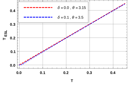
Figure 1: Here we depict $T_{\mathrm{E}SL}$ vs $T$, as given by (40), for the unitary dynamics governed by the Hamiltonian in (48) with the pure input $\Psi_{0}$ state and we have taken state parameter $p=0$ and Hamiltonian parameters $\{\delta=0.1,\theta=3.5\}$ and $\{\delta=0.0,\theta=3.15\}$.

In Fig. 1, we plot $T_{\mathrm{E}SL}$ vs $T$, as given by (40), for unitary dynamics generated by the two-qubit non-local Hamiltonian with Hamiltonian parameters $\{\delta=0.1,\theta=3.5\}$, and $\{\delta=0.0,\theta=3.15\}$ and state parameter $p=0$. For $\{\delta=0.0,\theta=3.15\}$, we have found that bound (40) is tight and attainable, whereas for $\{\delta=0.0,\theta=3.15\}$, bound (40) is almost tight.

Open system dynamics.– For the open system dynamics, under the Markovian approximation, Eq. (4) reduces to the following form  Lindblad (1976); Gorini et al. (1976):

$$\frac{\mathrm{d}\rho_{t}}{\mathrm{d}t}=-\iota[H,\rho_{t}]+\sum_{\alpha}\left(2L_{\alpha}\rho_{t}L^{{\dagger}}_{\alpha}-\{L^{{\dagger}}_{\alpha}L_{\alpha},\rho_{t}\}\right),$$ (55)

where $L_{\alpha}$’s are called the Lindbladian or quantum jump operators, $H$ is the driving Hamiltonian of the system and $\{A_{1},A_{2}\}:=A_{1}A_{2}+A_{2}A_{1}$ denotes the anti-commutator bracket. The above equation is called Gorini-Kossakowski-Lindblad-Sudarshan (GKLS) master equation.

We consider a bipartite system $AB$, where the subsystems $A$ and $B$ are qubits, each coupled with environments $E_{A}$ and $E_{B}$, respectively, where $E_{A}$ and $E_{B}$ are not interacting with each other. We assume that the system $AB$ is initialised in a pure state $\rho_{0}$ of the form

$$\rho_{0} =p\outerproduct{00}{00}+\sqrt{\left(1-p\right)p}(\outerproduct{00}{11}+\outerproduct{11}{00})$$

$$\hskip 9.95863pt+\left(1-p\right)\outerproduct{11}{11},$$ (56)

where $p\in[0,1]$. The CSS ( with respect to REE) of the above state is given by $\sigma^{*}_{0}=p\outerproduct{00}{00}+(1-p)\outerproduct{11}{11}$ Vedral et al. (1997).

We consider a pure dephasing channel as an example of a quantum correlation degradation process. The quantum jump operators for a pure dephasing process are given as $L_{1}=\sqrt{\frac{\gamma^{A}}{2}}\sigma^{A}_{z}\otimes\mathcal{I}_{B}$ and $L_{2}=\sqrt{\frac{\gamma^{B}}{2}}\mathcal{I}_{A}\otimes\sigma^{B}_{z}$, where $\sigma^{A}_{z}$ and $\sigma^{B}_{z}$ are Pauli operators acting on systems $A$ and $B$, respectively, and $\gamma^{A},\gamma^{B}$ both are real parameters denoting the strength of the dephasing process. The GKLS master equation governs time-evolution of the state $\rho_{t}$, and is given by

$$\frac{\mathrm{d}}{{\mathrm{d}}t}\rho_{t} =\gamma^{A}\left(\sigma^{A}_{z}\otimes\mathcal{I}_{B}\left(\rho_{t}\right)\sigma^{A}_{z}\otimes\mathcal{I}_{B}-\rho^{AB}_{t}\right)$$

$$\hskip 9.95863pt+\gamma^{B}\left(\mathcal{I}_{A}\otimes\sigma^{B}_{z}\left(\rho^{AB}_{t}\right)\mathcal{I}_{A}\otimes\sigma^{B}_{z}-\rho_{t}\right).$$ (57)

The state of the quantum system $AB$ at time $t$ is given by

$$\rho_{t} =p\outerproduct{00}{00}+\sqrt{p\left(1-p\right)}{\mathrm{e}}^{-4\gamma t}\left(\outerproduct{00}{11}+\outerproduct{11}{00}\right)$$

$$\hskip 9.95863pt+\left(1-p\right)\outerproduct{11}{11}$$ (58)

where we have assumed that the dephasing rates of both environments are equal to $\gamma$. The CSS at $t=0$ is given by $\sigma^{*}_{0}=p\outerproduct{00}{00}+(1-p)\outerproduct{11}{11}$. The pure dephasing process is a separable operation, so that the operation itself is its closest separable operation. Now, the CSS at time $t$ is given by

$$\sigma^{*}_{t}=p\outerproduct{00}{00}\left(1-p\right)\outerproduct{11}{11}.$$ (59)

To calculate bound (29), we have to calculate the following quantities

$$\mathcal{F}_{E}(0) =-p\log(p)-(1-p)\log(1-p),$$

$$\mathcal{F}_{E}(t) =h(p,t,\theta,\delta),$$ (60)

$$\left|\operatorname{tr}(\rho_{t}G_{\sigma_{t}}(\dot{\sigma}_{t}))\right| =0,$$ (61)

$$\norm{\mathcal{L}_{t}({\rho_{t}})}_{\mathrm{2}} =4\sqrt{2}\sqrt{\gamma^{2}(1-p)pe^{-8\gamma t}},$$ (62)

where $h(p,t,\theta,\delta)$ is function of $p$, $t$, $\theta$, and $\delta$. The analytic expression of $h(p,t,\theta,\delta)$ is given in Appendix B. For $p=\frac{1}{2}$ we have

$$\norm{\ln\rho_{t}-\ln\sigma_{t}}_{\mathrm{2}} =\sqrt{2}\sqrt{k_{1}+4\tanh^{-1}\left(e^{-4\gamma t}\right)^{2}},$$ (63)

where $k_{1}:=\left(\log\left(e^{-4\gamma t}+1\right)+\log\left(\frac{1}{2}-\frac{1}{2}e^{-4\gamma t}\right)\right)^{2}.$ Using bound (29) leads to

$$\scalebox{0.9}{\mbox{$\displaystyle T\geq\frac{|{h(p,T,\theta,\delta)+p\log(p)+(1-p)\log(1-p)|}}{8\int_{0}^{T}\sqrt{\left(\gamma^{2}(1-p)pe^{-8\gamma t}\right)\left(k_{1}+4\tanh^{-1}\left(e^{-4\gamma t}\right)^{2}\right)}\mathrm{d}t}$}}.$$ (64)

The speed limit bound in this case is not attainable.

VI conclusion

We have derived distinct speed limits on entanglement for both unitary and arbitrary dynamics using different measures of entanglement. Our approach relied on the assumption that the dynamics of the closest separable state can be described, or at least “faithfully” mimicked by the closest separable dynamical map of a given dynamical map. We have found that the upper bound on the entanglement rate of bipartite quantum systems depends on two key factors: the system’s evolution speed and a time-dependent term (due to the evolution of the CSS) that applies to both unitary and arbitrary completely positive and trace preserving (CPTP) dynamics. The speed limits on entanglement are fundamentally different from traditional speed limits of state evolution, as it is based on the rate of change of entanglement between subsystems rather than the rate of change in the distinguishability of the initial and evolved states of a system. It is important to identify, understand, and possibly exploit this difference, given that entanglement plays a critical role in quantum information processing, quantum communication, and quantum sensing, and its efficient manipulation and generation is key to the development of quantum technologies. By setting a fundamental limit on the rate at which entanglement can be generated or manipulated in bipartite systems, these speed limits provide a tool for evaluating the efficiency of different physical processes for generating and manipulating entanglement. Moreover, the speed limits determine the minimum time required to certain change in the amount entanglement of a bipartite system using any physical process. The speed limits on entanglement are closely related to entangling rates, which have been extensively studied for closed Dür et al. (2001); Mariën et al. (2016); Vershynina (2019); Gong and Hamazaki (2022); Hamilton and Clark (2023) and open bipartite systems Vershynina (2015). We found that the speed limits on entanglement for a two-qubit system governed by a non-local Hamiltonian are both tight and attainable. Our method can be used to find speed limits for other quantum resources and correlations as well (See Appendix C).

Appendix A Derivative of $f(t)=\operatorname{tr}(\rho_{t}\log\sigma_{t})$

We want to calculate derivative of the function $f(t)(=\operatorname{tr}(\rho_{t}\log\sigma_{t}))$ with respect time $t$. As we have assumed that derivative of $D\left(\rho_{t}\|\sigma_{t}\right)$ is well defined in $t\in I$, this also implies that $f(t)$ is smooth function of $t$ (i.e., $f(t)$ is continuous and differentiable) in the interval $I$. Then, $\frac{\mathrm{d}}{{\mathrm{d}}t}f(t)$ can be written as

$$\frac{\mathrm{d}}{{\mathrm{d}}t}f(t)=\lim_{\epsilon\rightarrow 0}\frac{f(t+\epsilon)-f(t)}{\epsilon}.$$ (65)

where $\epsilon$ is a small positive real number. The term $f(t+\epsilon)$ can be calculated by Taylor expansion ( after ignoring the higher order terms in $\epsilon$)

$$f(t+\epsilon) =\operatorname{tr}\left((\rho_{t}+\epsilon\dot{\rho}_{t})\log(\sigma_{t}+\epsilon\dot{\sigma}_{t})\right)$$

$$=\scalebox{0.95}{\mbox{$\displaystyle\operatorname{tr}\left(\rho_{t}\log(\sigma_{t}+\epsilon\dot{\sigma}_{t}))+\epsilon\operatorname{tr}(\dot{\rho}_{t}\log(\sigma_{t}+\epsilon\dot{\sigma}_{t})\right)$}}.$$ (66)

We now calculate $\log(\sigma_{t}+\epsilon\dot{\sigma}_{t})$ separately. Consider a small real number q in the $\delta$ neighbourhood of $0$, i.e., $q\in(-\delta,\delta)$, and two hermitian operators $A\in{\mathcal{L}}({\mathcal{H}})_{+}$, $B\in{\mathcal{L}}({\mathcal{H}})$ such that operator $A$ is full rank, then the Rellich’s theorem Kato (2013) says that $\log(A+qB)$ will be analytic in $q$. We then have the Taylor expansion

$$\log(A+qB)=\log A+qG_{A}(B)+O(q^{2}),$$ (67)

where $G_{A}(B)$ is the following self-adjoint linear operator: Working in the eigenbasis of $A=SMS^{-1}$, where $M={\mathrm{d}iag}(a_{1},a_{2},..a_{{\mathrm{d}im(\mathcal{H})}})$ is a diagonal matrix with eigenvalues of $A$ as its elements, define the matrices:

$$T_{kl}(A)=\frac{\log a_{k}-\log a_{l}}{a_{k}-a_{l}}$$ (68)

$$S_{ij}(A)=\frac{a_{i}-a_{j}}{\log a_{i}-\log a_{j}}.$$ (69)

Here we assume that $\frac{\log a-\log a}{a-a}=\frac{1}{a}$. Then, $G_{\alpha}(\beta)=\beta\circ T(\alpha)$, where $A\circ B$ is the component wise product of A and B, also known as Hadamard product. Note that in the case of singular $A$, Eq. (67) is not well defined but the following still holds Friedland and Gour (2011)

$$\scalebox{0.9}{\mbox{$\displaystyle\operatorname{tr}(C\log(A+qB))=\operatorname{tr}(C\log A)+q\operatorname{tr}(CG_{A}(B))+O(q^{2})$}},$$ (70)

assuming that $\operatorname{supp}(C)\subseteq\operatorname{supp}(A)$ for some $C\in{\mathcal{L}}(\mathcal{H})$ and operator $A+qB$ is full rank. In this scenario matrix elements of $T$ and $S$ are defined same as above (Eqs. (68) and (69)) on the support of $A$ and zero outside the support. If $A+qB$ is not full rank, but $\operatorname{supp}(C)\subseteq\operatorname{supp}(A+qB)$, then Eq. (70) can be modified as follows

$$\operatorname{tr}(C\Pi_{A+qB}\log(A+qB))= \operatorname{tr}(C\Pi_{A+qB}\log A)$$

$$\scalebox{0.92}{\mbox{$\displaystyle+q\operatorname{tr}(C\Pi_{A+qB}G_{A}(B))+O(q^{2})$}},$$ (71)

where $\Pi_{A+qB}$ is projection onto the support of operator $A+qB$. Since, we are only interested in the case where $A$ is either a density operator or derivative of a density operator, $C$ is a density operator and $B$ is a derivative of $C$. The above equation implies for $A=\sigma_{t}$, $C=\rho_{t}$, $B=\dot{\sigma}_{t}$ and $q=\epsilon$

$$\operatorname{tr}(\rho_{t}\Pi_{\sigma_{t}}\log(\sigma_{t}+\epsilon\dot{\sigma}_{t}))= \operatorname{tr}(\rho_{t}\Pi_{\sigma_{t}}\log\sigma_{t})+\epsilon\operatorname{tr}(\rho_{t}\Pi_{\sigma_{t}}G_{{\sigma}_{t}}(\dot{\sigma}_{t}))$$

$$+O(\epsilon^{2}),$$ (72)

where we have used the fact that for finite-dimensional Hilbert space, the support of $\dot{\sigma_{t}}$ is contained in $\sigma_{t}$, so instead of $\Pi_{\sigma_{t}+\epsilon\dot{\sigma_{t}}}$ we have used $\Pi_{\sigma_{t}}$. We have further assumed that $\dot{\sigma}_{t}$ is well-defined  (by this, we mean that each matrix element of $\sigma_{t}$ is differentiable with respect to $t$). The above equation gives the first term on the right hand side of Eq. (66). To calculate the second term, we take $A=\sigma_{t}$, $C=\dot{\rho_{t}}$, $B=\dot{\sigma}_{t}$ and $q=\epsilon$ in Eq. (71), we then get

$$\epsilon\operatorname{tr}(\dot{\rho_{t}}\Pi_{\sigma_{t}}\log(\sigma_{t}+\epsilon\dot{\sigma}_{t}))= \epsilon\operatorname{tr}(\rho_{t}\Pi_{\sigma_{t}}\log\sigma_{t})+O(\epsilon^{2}).$$ (73)

From Eqs. (65), (66),  (72), and  (73), we obtain ( after taking the limit $\epsilon\rightarrow 0$ and ignoring the terms of $O(\epsilon^{2})$):

$$\frac{{\mathrm{d}}}{{\mathrm{d}}t}f(t)=\operatorname{tr}(\dot{\rho_{t}}{\Pi}_{\sigma_{t}}\log\sigma_{t})+\operatorname{tr}(\rho_{t}{\Pi}_{\sigma_{t}}G_{\sigma_{t}}(\dot{\sigma}_{t})).$$ (74)

Appendix B expression for $h(p,t,\theta,\delta)$

The function $h(p,t,\theta,\delta)$ is defined as

$$h(p,t,\theta,\delta) :=\frac{e^{-4\gamma t}}{2\sqrt{a}}\left(\right.-(p-1)\left(\sqrt{a}e^{4\gamma t}+(2p-1)e^{8\gamma t}-2p\right)\log\left(a1\right)-(p-1)\left(\sqrt{a}e^{4\gamma t}+(1-2p)e^{8\gamma t}+2p\right)\log\left(a2\right)$$

$$\hskip 9.95863pt+p\left(\sqrt{a}e^{4\gamma t}+(1-2p)e^{8\gamma t}+2(p-1)\right)\log\left(a3\right)+p\left(\sqrt{a}e^{4\gamma t}+(2p-1)e^{8\gamma t}-2p+2\right)\log\left(a4\right)\left.\right),$$ (75)

where

$$a :=(1-2p)^{2}e^{8\gamma t}-4(p-1)p$$ (76)

$$a1 :=\frac{e^{-4\gamma t}\left(\sqrt{a}-e^{4\gamma t}\right)}{2(p-1)}$$ (77)

$$a2 :=-\frac{e^{-4\gamma t}\left(\sqrt{a}+e^{4\gamma t}\right)}{2(p-1)}$$ (78)

$$a3 :=\frac{e^{-4\gamma t}\left(e^{4\gamma t}-\sqrt{a}\right)}{2p}$$ (79)

$$a4 :=\frac{e^{-4\gamma t}\left(\sqrt{a}+e^{4\gamma t}\right)}{2p}$$ (80)

Appendix C Speed limits on general quantum resources

A similar analysis can also be done for other quantum resources if we take take relative entropy as a measure of distance, then the resource value of a given state $\rho$ is given as Chitambar and G. (2019):

$$R(\rho)= \min_{\sigma\in F}D(\rho\|\sigma)$$ (81)

$$=D(\rho\|\sigma^{*}),$$ (82)

where $F$ is the set of free states (i.e., states with zero resource value) and $\sigma^{*}\in F$ is a state which realizes the minimum of Eq. (81), called closest free state. Now, for that given dynamics of $\rho$, we have to find its closest dynamics which maps set of free states to free states. For the given initial state, if the closest free state is known, then, the maximal rate of resource variation and speed limit bound on the resource can be calculated in a similar way (as we have calculated for relative entropy of entanglement). In this case bounds on resource similar to (31) and (32) will provide a lower bound on the minimum time system will take to create (starting from free state) or fully deplete a certain amount of resource. We note that speed limits on resource for arbitrary dynamics have been studied earlier using relative entropy as resource measure Campaioli et al. (2022). For any dynamical system with associated Hilbert space $\mathcal{H}$, the state of the system depends on time. So, in general, the closest free state will also be time-dependent. The speed limit bounds in Campaioli et al. (2022) are obtained on the assumption that during the entire evolution period, the closest free state is not evolving. In our analysis, we assume that the evolution of the closest free state is governed by the closest free operation (map) (closest to the actual operation (map) governing the evolution of the state).

References

- Mandelstam and Tamm (1945) L. Mandelstam and IG Tamm, “The uncertainty relation between energy and time in non-relativistic quantum mechanics,” J. Phys. (USSR) 9, 249 (1945).
- Margolus and Levitin (1998) N. Margolus and L. B. Levitin, “The maximum speed of dynamical evolution,” Physica D: Nonlinear Phenomena 120, 188–195 (1998).
- Anandan and Aharonov (1990) J. Anandan and Y. Aharonov, “Geometry of quantum evolution,” Physical Review Letters 65, 1697–1700 (1990).
- Pati et al. (2023) A. K. Pati, B. Mohan, Sahil, and S. L. Braunstein, “Stronger quantum speed limit,” arXiv:2305.03839 (2023).
- Thakuria and Pati (2022) D. Thakuria and A. K. Pati, “Stronger quantum speed limit,” arXiv:2208.05469 (2022).
- Uhlmann (1992) A. Uhlmann, “An energy dispersion estimate,” Physics Letters A 161, 329–331 (1992).
- Giovannetti et al. (2004) V. Giovannetti, S. Lloyd, and L. Maccone, “The speed limit of quantum unitary evolution,” Journal of Optics B: Quantum and Semiclassical Optics 6, S807 (2004).
- J and Hernández (2022) S. Canseco J and A. V. Hernández, “Speed of evolution in entangled fermionic systems,” Journal of Physics A: Mathematical and Theoretical 55, 405301 (2022).
- Krisnanda et al. (2022) T. Krisnanda, S. Lee, C. Noh, J. Kim, A. Streltsov, T. C. H. Liew, and T. Paterek, “Correlations and energy in mediated dynamics,” New Journal of Physics 24, 123025 (2022).
- Shiraishi and Saito (2021) N. Shiraishi and K. Saito, “Speed limit for open systems coupled to general environments,” Physical Review Research 3, 023074 (2021).
- Funo et al. (2019) K. Funo, N. Shiraishi, and K. Saito, “Speed limit for open quantum systems,” New Journal of Physics 21, 013006 (2019).
- Van Vu and Saito (2023) T. Van Vu and K. Saito, “Topological speed limit,” Physical Review Letters 130, 010402 (2023).
- Pires et al. (2016) D. P. Pires, M. Cianciaruso, L. C. Céleri, G. Adesso, and D. O. Soares-Pinto, “Generalized geometric quantum speed limits,” Physical Review X 6, 021031 (2016).
- Brody and Longstaff (2019) D. C. Brody and B. Longstaff, “Evolution speed of open quantum dynamics,” Physical Review Research 1 (2019), 10.1103/physrevresearch.1.033127.
- Taddei et al. (2013) M. M. Taddei, B. M. Escher, L. Davidovich, and R. L. de Matos Filho, “Quantum speed limit for physical processes,” Physical Review Letters 110, 050402 (2013).
- del Campo et al. (2013) A. del Campo, I. L. Egusquiza, M. B. Plenio, and S. F. Huelga, “Quantum speed limits in open system dynamics,” Physical Review Letters 110, 050403 (2013).
- Campaioli et al. (2013) F. Campaioli, F.A. Pollock, and K. Modi, “Quantum speed limits in open system dynamics,” Quantum 3, 168 (2013).
- Deffner and Lutz (2013) S. Deffner and E. Lutz, “Quantum speed limit for non-markovian dynamics,” Physical Review Letters 111, 010402 (2013).
- Kiselev et al. (2022) A. D. Kiselev, Ali R., and A. V. Rybin, “Speed of evolution and correlations in multi-mode bosonic systems,” Entropy, 24 (2022).
- Thakuria et al. (2022) D. Thakuria, A. Srivastav, B. Mohan, A. Kumari, and A. K. Pati, “Generalised quantum speed limit for arbitrary evolution,” arXiv:2207.04124 (2022).
- Ashhab et al. (2012) S. Ashhab, P. C. de Groot, and F. Nori, “Speed limits for quantum gates in multiqubit systems,” Physical Review A 85, 052327 (2012).
- Aifer and Deffner (2022) M. Aifer and S. Deffner, “From quantum speed limits to energy-efficient quantum gates,” New Journal of Physics 24, 055002 (2022).
- Campbell et al. (2018) S. Campbell, M. G Genoni, and S. Deffner, “Precision thermometry and the quantum speed limit,” Quantum Science and Technology 3, 025002 (2018).
- Beau and del Campo (2017) M. Beau and A. del Campo, “Nonlinear quantum metrology of many-body open systems,” Physical Review Letters 119, 010403 (2017).
- Caneva et al. (2009) T. Caneva, M. Murphy, T. Calarco, R. Fazio, S. Montangero, V. Giovannetti, and G. E. Santoro, “Optimal control at the quantum speed limit,” Physical Review Letters 103, 240501 (2009).
- Deffner and Campbell (2017) S. Deffner and S. Campbell, “Quantum speed limits: from heisenberg’s uncertainty principle to optimal quantum control,” Journal of Physics A: Mathematical and Theoretical 50, 453001 (2017).
- Murphy et al. (2010) M. Murphy, S. Montangero, V. Giovannetti, and T. Calarco, “Communication at the quantum speed limit along a spin chain,” Physical Review A 82, 022318 (2010).
- Mohan and Pati (2021) B. Mohan and A. K. Pati, “Reverse quantum speed limit: How slowly a quantum battery can discharge,” Physical Review A 104, 042209 (2021).
- Mohan and Pati (2022) B. Mohan and A. K. Pati, “Quantum speed limits for observables,” Physical Review A 106, 042436 (2022).
- Campaioli et al. (2017) F. Campaioli, F. A. Pollock, F. C. Binder, L. Céleri, J. Goold, S. Vinjanampathy, and K. Modi, “Enhancing the charging power of quantum batteries,” Physical Review Letters 118, 150601 (2017).
- Mukhopadhyay et al. (2018) C. Mukhopadhyay, A. Misra, S. Bhattacharya, and Arun Kumar Pati, “Quantum speed limit constraints on a nanoscale autonomous refrigerator,” Physical Review E 97, 062116 (2018).
- Einstein et al. (1935) A. Einstein, B. Podolsky, and N. Rosen, “Can quantum-mechanical description of physical reality be considered complete?” Physical Review 47, 777–780 (1935).
- Bell (1964) J. S. Bell, “On the Einstein Podolsky Rosen paradox,” Physics Physique Fizika 1, 195–200 (1964).
- Bennett et al. (1993) C. H. Bennett, G. Brassard, C. Crépeau, R. Jozsa, A. Peres, and W. K. Wootters, “Teleporting an unknown quantum state via dual classical and einstein-podolsky-rosen channels,” Physical Review Letters 70, 1895–1899 (1993).
- Bennett and Wiesner (1992) C. H. Bennett and S. J. Wiesner, “Communication via one- and two-particle operators on einstein-podolsky-rosen states,” Physical Review Letters 69, 2881–2884 (1992).
- Ekert (1991) A. K. Ekert, “Quantum cryptography based on bell’s theorem,” Physical Review Letters 67, 661–663 (1991).
- Jozsa (1997) R. Jozsa, “Entanglement and quantum computation,” quant-ph/9707034 (1997).
- Jozsa and Linden (2003) R. Jozsa and N. Linden, “On the role of entanglement in quantum-computational speed-up,” Proceedings of the Royal Society of London. Series A: Mathematical, Physical and Engineering Sciences 459, 2011–2032 (2003).
- Colbeck and Renner (2012) R. Colbeck and R. Renner, “Free randomness can be amplified,” Nature Physics 8, 450–453 (2012).
- Dowling (2008) J. P. Dowling, “Quantum optical metrology – the lowdown on high-N00N states,” Contemporary Physics 49, 125–143 (2008).
- Ho and Abanin (2017) W. W. Ho and D. A. Abanin, “Entanglement dynamics in quantum many-body systems,” Physical Review B 95, 094302 (2017).
- Elsayed et al. (2018) T. A. Elsayed, K. Mølmer, and L. Bojer Madsen, “Entangled quantum dynamics of many-body systems using bohmian trajectories,” Scientific Reports 8 (2018), 10.1038/s41598-018-30730-0.
- Brandão et al. (2020) I. Brandão, B. Suassuna, B. Melo, and T. Guerreiro, “Entanglement dynamics in dispersive optomechanics: Nonclassicality and revival,” Physical Review Research 2, 043421 (2020).
- Gong and Hamazaki (2022) Z. Gong and R. Hamazaki, “Bounds in nonequilibrium quantum dynamics,” International Journal of Modern Physics B 36 (2022), 10.1142/s0217979222300079.
- Hamazaki (2023) Ryusuke Hamazaki, “Quantum velocity limits for multiple observables: Conservation laws, correlations, and macroscopic systems,” arXiv:2305.03190 (2023).
- García-Pintos et al. (2022) L. P. García-Pintos, S. B. Nicholson, J. R. Green, A. del Campo, and A. V. Gorshkov, “Unifying quantum and classical speed limits on observables,” Physical Review X 12, 011038 (2022).
- Hamazaki (2022) R. Hamazaki, “Speed limits for macroscopic transitions,” PRX Quantum 3, 020319 (2022).
- Hörnedal et al. (2023) N. Hörnedal, N. Carabba, K. Takahashi, and A. del Campo, “Geometric operator quantum speed limit, wegner hamiltonian flow and operator growth,” (2023).
- Carabba et al. (2022) N. Carabba, N. Hörnedal, and A. del Campo, “Quantum speed limits on operator flows and correlation functions,” Quantum 6, 884 (2022).
- Hasegawa (2023) Y. Hasegawa, “Thermodynamic correlation inequality,” arXiv:2301.03060 (2023).
- Jing et al. (2016) J. Jing, L. Wu, and A. del Campo, “Fundamental speed limits to the generation of quantumness,” Scientific Reports 6 (2016), 10.1038/srep38149.
- Mohan et al. (2022) B. Mohan, S. Das, and A. K. Pati, “Quantum speed limits for information and coherence,” New Journal of Physics 24, 065003 (2022).
- Bera et al. (2013) M. N. Bera, R Prabhu, A. K. Pati, A. Sen De, and U. Sen, “Limit on time-energy uncertainty with multipartite entanglement,” arXiv:1303.0706 (2013).
- Rudnicki (2021) L. Rudnicki, “Quantum speed limit and geometric measure of entanglement,” Physical Review A 104, 032417 (2021).
- Pandey et al. (2023) V. Pandey, D. Shrimali, B. Mohan, S. Das, and A. K. Pati, “Speed limits on correlations in bipartite quantum systems,” Physical Review A 107, 052419 (2023).
- Shrimali et al. (2022) D. Shrimali, S. Bhowmick, V. Pandey, and A. K. Pati, “Capacity of entanglement for a nonlocal hamiltonian,” Physical Review A 106, 042419 (2022).
- Campaioli et al. (2022) F. Campaioli, C. Yu, F. A Pollock, and K. Modi, “Resource speed limits: maximal rate of resource variation,” New Journal of Physics 24, 065001 (2022).
- Pires (2022) D. P. Pires, “Unified entropies and quantum speed limits for nonunitary dynamics,” Physical Review A 106, 012403 (2022).
- Pires et al. (2021) D. P. Pires, K. Modi, and L. Chibebe Cé leri, “Bounding generalized relative entropies: Nonasymptotic quantum speed limits,” Physical Review E 103 (2021), 10.1103/physreve.103.032105.
- Paulson and Banerjee (2022) K. G Paulson and S. Banerjee, “Quantum speed limit for the creation and decay of quantum correlations,” (2022).
- (61) A. Shaham, A. Halevy, L. Dovrat, E. Megidish, and H. S. Eisenberg, “Entanglement dynamics in the presence of controlled unital noise,” Scientific Reports 5, 10796.
- Nosrati et al. (2020) F. Nosrati, A. Castellini, G. Compagno, and R. Lo Franco, “Robust entanglement preparation against noise by controlling spatial indistinguishability,” npj Quantum Information 6 (2020), 10.1038/s41534-020-0271-7.
- Schachenmayer et al. (2013) J. Schachenmayer, B. P. Lanyon, C. F. Roos, and A. J. Daley, “Entanglement growth in quench dynamics with variable range interactions,” Physical Review X 3, 031015 (2013).
- Hamilton and Clark (2023) Gregory A. Hamilton and Bryan K. Clark, “Quantifying unitary flow efficiency and entanglement for many-body localization,” Physical Review B 107, 064203 (2023).
- Horodecki et al. (1998) M. Horodecki, P. Horodecki, and R. Horodecki, “Mixed-state entanglement and distillation: Is there a “bound” entanglement in nature?” Physical Review Letters 80, 5239–5242 (1998).
- Vedral et al. (1997) V. Vedral, M. B. Plenio, M. A. Rippin, and P. L. Knight, “Quantifying entanglement,” Physical Review Letters 78, 2275–2279 (1997).
- Eisert et al. (2003) J. Eisert, K. Audenaert, and M. B. Plenio, “Remarks on entanglement measures and non-local state distinguishability,” Journal of Physics A: Mathematical and General 36, 5605–5615 (2003).
- Luo (2005) S. Luo, “Heisenberg uncertainty relation for mixed states,” Physical Review A 72, 042110 (2005).
- Robertson (1929) H. P. Robertson, “The uncertainty principle,” Phys. Rev. 34, 163 (1929).
- Rivas and Huelga (2012) A. Rivas and S. F. Huelga, Open quantum systems, Vol. 10 (Springer, 2012).
- Cirac et al. (2001) J. I. Cirac, W. Dür, B. Kraus, and M. Lewenstein, “Entangling operations and their implementation using a small amount of entanglement,” Physical Review Letters 86, 544–547 (2001).
- Umegaki (1962) H. Umegaki, “Conditional expectation in an operator algebra. IV. Entropy and information,” Kodai Mathematical Seminar Reports 14, 59 – 85 (1962).
- Werner (1989) R. F. Werner, “Quantum states with einstein-podolsky-rosen correlations admitting a hidden-variable model,” Physical Review A 40, 4277–4281 (1989).
- Bennett et al. (1996) C. H. Bennett, D. P. DiVincenzo, J. A. Smolin, and W. K. Wootters, “Mixed-state entanglement and quantum error correction,” Physical Review A 54, 3824–3851 (1996).
- Wootters (2001) W. K Wootters, “Entanglement of formation and concurrence,” Quantum Information and Computation 1, 27–44 (2001).
- Wootters (1998) W. K. Wootters, “Entanglement of formation of an arbitrary state of two qubits,” Physical Review Letters 80, 2245–2248 (1998).
- Vidal and Werner (2002) G. Vidal and R. F. Werner, “Computable measure of entanglement,” Physical Review A 65, 032314 (2002).
- Vedral and Plenio (1998) V. Vedral and M. B. Plenio, “Entanglement measures and purification procedures,” Physical Review A 57, 1619–1633 (1998).
- Friedland and Gour (2011) S. Friedland and G. Gour, “An explicit expression for the relative entropy of entanglement in all dimensions,” Journal of Mathematical Physics 52, 052201 (2011).
- Das et al. (2021) S. Das, S. Bäuml, M. Winczewski, and K. Horodecki, “Universal limitations on quantum key distribution over a network,” Physical Review X 11, 041016 (2021).
- Das et al. (2018) S. Das, S. Khatri, G. Siopsis, and M. M Wilde, “Fundamental limits on quantum dynamics based on entropy change,” Journal of Mathematical Physics 59, 012205 (2018).
- Campaioli et al. (2019) F. Campaioli, F. A. Pollock, and K. Modi, “Tight, robust, and feasible quantum speed limits for open dynamics,” Quantum 3, 168 (2019).
- Sakuldee and Rudnicki (2023) F. Sakuldee and L. Rudnicki, “Bounds on the breaking time for entanglement-breaking channels,” Physical Review A 107, 022430 (2023).
- Lindblad (1976) G. Lindblad, “On the generators of quantum dynamical semigroups,” Communications in Mathematical Physics 48, 119–130 (1976).
- Gorini et al. (1976) V. Gorini, A. Kossakowski, G. Sudarshan, and E. Chandy, “Completely positive dynamical semigroups of N‐level systems,” Journal of Mathematical Physics 17, 821–825 (1976).
- Dür et al. (2001) W. Dür, G. Vidal, J. I. Cirac, N. Linden, and S. Popescu, “Entanglement capabilities of nonlocal hamiltonians,” Physical Review Letters 87, 137901 (2001).
- Mariën et al. (2016) M. Mariën, K. M.R. Audenaert, K. Van Acoleyen, and F. Verstraete, “Entanglement rates and the stability of the area law for the entanglement entropy,” Communications in Mathematical Physics 346, 35–73 (2016).
- Vershynina (2019) A. Vershynina, “Entanglement rates for rényi, tsallis, and other entropies,” Journal of Mathematical Physics 60, 022201 (2019).
- Vershynina (2015) A. Vershynina, “Entanglement rates for bipartite open systems,” Physical Review A 92, 022311 (2015).
- Kato (2013) T. Kato, Perturbation theory for linear operators, Vol. 132 (Springer Science & Business Media, 2013).
- Chitambar and G. (2019) E. Chitambar and Gilad G., “Quantum resource theories,” Reviews of Modern Physics 91, 025001 (2019).