Quark pair angular correlations in the proton: entropy versus entanglement negativity

Abstract

Two-particle correlations in the proton on the light-front are described by a mixed density matrix obtained by tracing over all other, unobserved, degrees of freedom. We quantify genuinely quantum quark azimuthal correlations in terms of the entanglement negativity measure of Quantum Information Theory. While the two-quark state in color space is one of high entropy and weak quantum correlation, we find that a standard three-quark model wave function from the literature predicts an azimuthally correlated state of low entropy and high entanglement negativity. Low entropy is consistent with expectations for many colors (at fixed ’t Hooft coupling $g^{2}{N_{\mathrm{c}}}$) but high negativity indicates substantial two-particle quantum correlations at ${N_{\mathrm{c}}}=3$. We show that suppressing quantum correlations associated with entanglement negativity strongly modifies quark pair azimuthal moments $\langle\zeta^{n}\rangle$, $\zeta=\exp(i(\phi_{1}-\phi_{2}))$, intrinsic to the proton state.
We also describe how to account for the leading ${\cal O}(g^{2})$ correction to the density matrix from light-cone perturbation theory which is due to the presence (or exchange) of a gluon in the proton. This correction increases the entropy and reduces the negativity of the density matrix for quark pair azimuthal correlations. Hence, the entanglement negativity measure may provide novel insight into the structure of the proton state of QCD.

I Introduction

Entanglement, a quantum correlation in superposition states, is generally regarded to be the most striking break of the quantum theory of matter and radiation from classical theory [1, 2, 3]. In a light-front Fock state description of the proton, each Fock state corresponds to a superposition of partons, quarks, anti-quarks, and gluons, of all possible combinations of colors, flavors, spins, and momenta. Entanglement of various degrees of freedom in the proton is currently under intense scrutiny [4, 5, 6, 7, 8, 9, 10, 11, 12, 13, 14, 15, 16, 17, 18, 19, 20, 21, 22, 23, 24, 25, 26, 27]. One usually starts from the pure proton state and traces over various unobserved degrees of freedom, the “environment”, to obtain a reduced density matrix for the remaining “system”:

$$\rho_{s}=\,\mathrm{tr}_{e}\,\rho~{}.$$ (1)

In general, $\rho_{s}$ represents a mixed state. In this setting of “bi-partite entanglement” the magnitude of entanglement, i.e. of quantum correlations, of the remaining degrees of freedom of the system with those of the environment can be quantified, for example, in terms of the von Neumann entropy $S(\rho_{s})$. A pure state is entangled if and only if the von Neumann entropy of the partial state $\rho_{s}$ is nonzero.

Our present focus is different. After tracing out the environment, we divide further the remaining system into two systems $s_{1}$ and $s_{2}$. We are interested in the sub-subsystem correlations of $s_{1}$ and $s_{2}$, specifically in azimuthal quark pair correlations in the proton, and whether these are quantum or classical, in the sense of Quantum Information Theory. The entanglement of $s_{1}$ with $s_{2}$ can not be measured via $S(\rho_{s_{1}})$ or $S(\rho_{s_{2}})$ because $\rho_{s}$ is not a pure state: these entropies are also sensitive to classical correlations among the remaining two subsystems. Instead, we shall quantify the magnitude of quantum correlations through the entanglement negativity of $\rho_{s}$ [28, 29]. A brief introduction into separable states and quantum correlations can be found in appendix A.

II Color correlations

We first present a simple yet instructive example. We start from a fully antisymmetric state of ${N_{\mathrm{c}}}\geq 2$ color charges in the fundamental representation of color-$SU({N_{\mathrm{c}}})$:

$$\rho_{i_{1}\ldots i_{N_{\mathrm{c}}},i^{\prime}_{1}\ldots i^{\prime}_{N_{\mathrm{c}}}}=\frac{1}{{N_{\mathrm{c}}}!}\,\epsilon^{i_{1}\ldots i_{N_{\mathrm{c}}}}\epsilon^{i^{\prime}_{1}\ldots i^{\prime}_{N_{\mathrm{c}}}}~{}.$$ (2)

Tracing over all but two degrees of freedom yields the two-subsystem reduced density matrix

$$\rho_{ij,i^{\prime}j^{\prime}}=\frac{1}{{N_{\mathrm{c}}}({N_{\mathrm{c}}}-1)}\left(\delta_{ii^{\prime}}\delta_{jj^{\prime}}-\delta_{ij^{\prime}}\delta_{i^{\prime}j}\right)~{}.$$ (3)

For $N_{c}\to\infty$, at leading order in $1/N_{c}$ this reduces to a product state

$$\rho^{\mathrm{LO}}_{ij,i^{\prime}j^{\prime}}=\frac{1}{{N_{\mathrm{c}}}^{2}}\delta_{ii^{\prime}}\delta_{jj^{\prime}}~{}.$$ (4)

This state lacks correlations, and also is not in general anti-symmetric under $i\leftrightarrow j$ (or $i^{\prime}\leftrightarrow j^{\prime}$). The von Neumann entropy for this matrix is $S^{\mathrm{LO}}=2\log{N_{\mathrm{c}}}$, twice the entropy for a single fundamental color charge, i.e. the leading contribution to $S$ is extensive and scales with the number of charges.

Correlations emerge at next-to-leading order,

$$\rho^{\mathrm{NLO}}_{ij,i^{\prime}j^{\prime}}=\frac{1}{{N_{\mathrm{c}}}^{2}}\left(\frac{{N_{\mathrm{c}}}+1}{{N_{\mathrm{c}}}}\delta_{ii^{\prime}}\delta_{jj^{\prime}}-\delta_{ij^{\prime}}\delta_{i^{\prime}j}\right)~{}.$$ (5)

This density matrix does satisfy anti-symmetry, at leading order in $1/{N_{\mathrm{c}}}$. Its two eigenvalues are $\lambda_{1}=1/{N_{\mathrm{c}}}^{3}$ and $\lambda_{2}=(2+\frac{1}{{N_{\mathrm{c}}}})/{N_{\mathrm{c}}}^{2}$, with multiplicities $N_{1}={N_{\mathrm{c}}}({N_{\mathrm{c}}}+1)/2$ and $N_{2}={N_{\mathrm{c}}}({N_{\mathrm{c}}}-1)/2$, respectively. Hence, the entropy is $S^{\mathrm{NLO}}=2\log{N_{\mathrm{c}}}-\log 2+\cdots$. The ${N_{\mathrm{c}}}$-independent correction arises because the leading $2\log{N_{\mathrm{c}}}$ overcounts the increase in the dimensionality of the Hilbert space from one to two color charges.

Indeed, the two-particle Hilbert space ${\cal H}\otimes{\cal H}={\cal H}_{S}\oplus{\cal H}_{A}$ decomposes into a direct sum of a symmetric and an anti-symmetric space, and the allowed state vectors belong to the latter. The dimension of ${\cal H}_{A}$ is

$${{{N_{\mathrm{c}}}}\choose{2}}=\frac{{N_{\mathrm{c}}}!}{2!\,({N_{\mathrm{c}}}-2)!}=\frac{1}{2}{N_{\mathrm{c}}}({N_{\mathrm{c}}}-1)~{},$$ (6)

since this is the number of linearly independent rank-2 anti-symmetric tensors over a ${N_{\mathrm{c}}}$-dimensional vector space. Hence, this is the number of non-zero eigenvalues of the exact $\rho$ from eq. (3). It is clear that all eigenvalues are equal, so $\lambda_{i}=2/{N_{\mathrm{c}}}({N_{\mathrm{c}}}-1)$. This can be confirmed by explicit computation using standard techniques.

The purity of $\rho$ is $\,\mathrm{tr}\,\rho^{2}=\sum_{\lambda}N_{\lambda}\lambda^{2}=\frac{2}{{N_{\mathrm{c}}}({N_{\mathrm{c}}}-1)}$, and the entropy is $S=-\sum_{\lambda}N_{\lambda}\lambda\log\lambda=\log[\frac{1}{2}{N_{\mathrm{c}}}({N_{\mathrm{c}}}-1)]$. For ${N_{\mathrm{c}}}=2$ the purity is $1$ and the entropy is $0$, since nothing has been traced over and $\rho$ is a pure state. For ${N_{\mathrm{c}}}\to\infty$, on the other hand,

$$S(\rho)=2\log{N_{\mathrm{c}}}-\log 2-\frac{1}{{N_{\mathrm{c}}}}-\frac{1}{2{N_{\mathrm{c}}}^{2}}+{\cal O}({N_{\mathrm{c}}}^{-3})~{},$$ (7)

which exhibits subleading corrections due to quantum correlations. Both terms, $-\log 2$ and $-{N_{\mathrm{c}}}^{-1}$, are associated with the existence of a negative eigenvalue of the partial transpose of $\rho$, as we discuss at the end of this section (and in appendix B).

Subsystem correlations may also be quantified in terms of the “coherent information” measure [30]. For a bipartite state $\rho$ it is defined as

$$I(2\rangle 1)\equiv S(\rho^{(1)})-S(\rho)~{},$$ (8)

where $\rho^{(1)}=\,\mathrm{tr}_{2}\rho$ is the reduced density matrix for system 1, and $S$ denotes the von Neumann entropy. $I(2\rangle 1)$ quantifies how much less is known about subsystem 1 than about the whole composed system [30]. In the presence of strong entanglement and low entropy one expects $I(2\rangle 1)>0$ and vice versa: if $\rho=\rho^{(1)}\otimes\rho^{(2)}$ then $S(\rho)=S(\rho^{(1)})+S(\rho^{(2)})$ and $I(2\rangle 1)=-S(\rho^{(2)})$.

For the density matrix (3), $\rho^{(1)}_{ii^{\prime}}={N_{\mathrm{c}}}^{-1}\delta_{ii^{\prime}}$, and

$$I(2\rangle 1)=\log\frac{2}{{N_{\mathrm{c}}}-1}=-\log{N_{\mathrm{c}}}+\log 2-\frac{1}{{N_{\mathrm{c}}}}-\frac{1}{2{N_{\mathrm{c}}}^{2}}+{\cal O}({N_{\mathrm{c}}}^{-3})~{}.$$ (9)

The leading contribution at large ${N_{\mathrm{c}}}$ is, of course, half the “ideal gas” entropy: dividing the system in half reduces the entropy by half. Hence, the negative coherent information indicates weak entanglement and high entropy of the reduced state.

The entanglement negativity is given by (minus) the sum of negative eigenvalues of the partial transpose over the second system $\rho^{T_{2}}$, which swaps $j$ and $j^{\prime}$ in eq. (3). The eigenvalues of $\rho^{T_{2}}$ are $-\frac{1}{{N_{\mathrm{c}}}}$ with multiplicity 1 and $\frac{1}{{N_{\mathrm{c}}}({N_{\mathrm{c}}}-1)}$ with multiplicity ${N_{\mathrm{c}}}^{2}-1$. This means that the negativity of $\rho$ is ${\cal N}(\rho)={1}/{{N_{\mathrm{c}}}}$, i.e. the inverse of the dimension of the Hilbert space for one fundamental charge. Hence, quantum correlations besides anti-symmetrization of the two remaining color charges are indeed ${\cal O}({N_{\mathrm{c}}}^{-1})$. In the limit of many colors, this agrees with the correlation entropy, i.e. the third term on the r.h.s. of eqs. (7) or (9). However, in this limit the overall entropy of the state (3) is far greater than its negativity and coherent information is negative.

III Light-cone wave functions and density matrices describing azimuthal correlations

We briefly introduce the light-cone Fock state description of the proton state. Much more detailed accounts can be found in the literature, e.g. refs. [31, 32, 33, 34].

A proton state with light-cone momentum $P^{+}$ and transverse momentum $\vec{P}_{\perp}=0$ is written as

$$|P\rangle=\sum_{n}\int{\rm d}\Phi_{n}\,\Psi_{n}(k_{1},\cdots,k_{n})\,|k_{1},\cdots,k_{n}\rangle~{}.$$ (10)

We have omitted writing the spin-flavor and color space structure since we will trace over those degrees of freedom. ${\rm d}\Phi_{n}$ denotes the integration measure over the $n$ on-shell parton three-momenta $k_{i}=(x_{i}P^{+},\vec{k}_{i})$, including $\delta$-functions which enforce $\sum x_{i}=1$ and $\sum\vec{k}_{i}=\vec{P}_{\perp}=0$. The amplitudes $\Psi_{n}(k_{1},\cdots,k_{n})$ are the $n$-parton light-cone wave functions. They are gauge invariant and universal (process independent), and are obtained, in principle, from the non-perturbative solution of the QCD Hamiltonian. The ket $|k_{1},\cdots,k_{n}\rangle$ is obtained by acting with the appropriate creation operators on the vacuum of the free theory, which in light-cone quantization coincides with the vacuum of the interacting theory.

To date, exact solutions for the light-cone wave functions are not available, of course. In the future, lattice gauge theory may provide numerical solutions for moderate parton momentum fractions $x_{i}$ and transverse momenta $\vec{k}_{i}$ via a large momentum expansion of equal-time Euclidean correlation functions in instant quantization [35, 36, 37]. In the following we shall rely on a truncation of Fock space and solutions of effective light-cone Hamiltonians supplemented by the ${\cal O}(g^{2})$ correction obtained from light-cone perturbation theory.

III.1 Three quark Fock state

Empirical observations suggest that at moderate momentum fractions $x_{i}\,\,\vbox{\hbox{$\buildrel\displaystyle>\over{\sim}$}}\,\,0.1$, and for transverse momenta up to a few times the QCD confinement scale, the light-cone momentum structure of the proton is described reasonably well by a “light front constituent quark model”. In this approximation, the light-cone state of the proton is written in terms of its three quark Fock state and an effective three quark wave function as follows:

$$|P\rangle = \int\limits_{[0,1]^{3}}\prod_{i=1\cdots 3}\frac{{\rm d}x_{i}}{2x_{i}}\,\delta\left(1-\sum_{i}x_{i}\right)\int\prod_{i=1\cdots 3}\frac{{\rm d}^{2}k_{i}}{(2\pi)^{3}}\,(2\pi)^{3}\,\delta\left(\sum_{i}\vec{k}_{i}\right)\,\Psi_{\mathrm{qqq}}\left(k_{1};k_{2};k_{3}\right)\,\,\left|k_{1};k_{2};k_{3}\right>$$ (11)

$$= \int\frac{{\rm d}x_{1}{\rm d}x_{2}}{2x_{1}\,2x_{2}\,2(1-x_{1}-x_{2})}\int\frac{{\rm d}^{2}k_{1}}{(2\pi)^{3}}\,\frac{{\rm d}^{2}k_{2}}{(2\pi)^{3}}\,\Psi_{\mathrm{qqq}}\left(x_{1},\vec{k}_{1};x_{2},\vec{k}_{2};1-x_{1}-x_{2},-\vec{k}_{1}-\vec{k}_{2}\right)$$

$$~{}~{}~{}~{}~{}~{}~{}~{}~{}~{}~{}~{}\left|x_{1},\vec{k}_{1};x_{2},\vec{k}_{2};1-x_{1}-x_{2},-\vec{k}_{1}-\vec{k}_{2}\right>~{}.$$

As already mentioned above we omit the spin-flavor and color space structures as we will focus on azimuthal correlations in momentum space. The spatial wave function $\Psi_{\mathrm{qqq}}$ is symmetric under exchange of any two quarks: $\Psi_{\mathrm{qqq}}\left(k_{1};k_{2};k_{3}\right)=\Psi_{\mathrm{qqq}}\left(k_{2};k_{1};k_{3}\right)$ etc. The second form of $|P\rangle$ shows that $k_{3}=(x_{3}P^{+},\vec{k}_{3})$ is not a degree of freedom, it has been eliminated by the COM constraint. Only $k_{1}$ and $k_{2}$ are degrees of freedom.

For numerical estimates below we employ a model due to Brodsky and Schlumpf [38, 34] which we briefly summarize for completeness. Alternative models which represent solutions of effective light-cone Hamiltonians with interactions can be found in the literature, e.g. refs. [39, 40].

The model of Brodsky and Schlumpf used here corresponds to

$$\Psi_{\mathrm{qqq}}\left(x_{i},\vec{k}_{i}\right)=N\,\sqrt{x_{1}x_{2}x_{3}}\,\,e^{-{\cal M}^{2}/2\beta^{2}}$$ (12)

where ${\cal M}^{2}=\sum(\vec{k}_{i}^{2}+m_{q}^{2})/x_{i}$ is the invariant mass squared of the non-interacting three-quark system [41]. It is understood that $x_{3}$ and $\vec{k}_{3}$ are short-hands for $1-x_{1}-x_{2}$ and $-\vec{k}_{1}-\vec{k}_{2}$, respectively. The normalization $N$ of this wave function follows from $\,\mathrm{tr}\,\rho=1$, see below. The non-perturbative parameters $m_{q}=0.26$ GeV and $\beta=0.55$ GeV have been tuned in ref. [34] to low-energy properties of the proton such as its “radius” (the inverse RMS quark transverse momentum).

From the above expression for $|P\rangle$ one obtains the density matrix

$$\rho_{\alpha\alpha^{\prime}}=\Psi_{\mathrm{qqq}}^{*}(k_{1}^{\prime},k_{2}^{\prime})\,\Psi_{\mathrm{qqq}}(k_{1},k_{2})~{},$$ (13)

where $\alpha=\{k_{1};k_{2}\}$, $\alpha^{\prime}=\{k_{1}^{\prime};k_{2}^{\prime}\}$; for a detailed presentation of the steps from eq. (11) to (13) see ref. [27]. Here, we have omitted the momenta of the third quarks from the arguments of the wave functions; they are understood to be such that the sums of transverse momenta are zero while the sums of light-cone momentum fractions are 1.

The trace measure is

$$\,\mathrm{tr}=\frac{1}{2}\int\frac{{\rm d}x_{1}{\rm d}x_{2}}{2x_{1}\,2x_{2}\,2(1-x_{1}-x_{2})}\int\frac{{\rm d}^{2}k_{1}}{(2\pi)^{3}}\,\frac{{\rm d}^{2}k_{2}}{(2\pi)^{3}}~{},$$ (14)

and this sets the normalization of the light-cone wave function.

III.2 Quark azimuthal angular correlations

Our main interest in this paper is in two-quark angular correlations. These are described by the density matrix $\rho_{\vec{k}_{1}\vec{k}_{2},\vec{k}_{1}^{\prime}\vec{k}_{2}^{\prime}}$ obtained by tracing over $x_{1}$ and $x_{2}$:

$$\rho_{\vec{k}_{1}\vec{k}_{2},\vec{k}_{1}^{\prime}\vec{k}_{2}^{\prime}}=\int\frac{{\rm d}x_{1}}{2x_{1}}\frac{{\rm d}x_{2}}{2x_{2}(1-x_{1}-x_{2})}\,\Psi^{*}(x_{1},x_{2},\vec{k}_{1}^{\prime},\vec{k}_{2}^{\prime})\,\Psi(x_{1},x_{2},\vec{k}_{1},\vec{k}_{2})~{}.$$ (15)

To reduce the dimension of the matrix we can also trace over $|\vec{k}_{1}|$ and $|\vec{k}_{2}|$ to obtain

$$\rho_{\phi_{1}\phi_{2},\phi_{1}^{\prime}\phi_{2}^{\prime}}=\int|\vec{k}_{1}|\,\frac{{\rm d}|\vec{k}_{1}|}{16\pi^{3}}\,|\vec{k}_{2}|\,\frac{{\rm d}|\vec{k}_{2}|}{16\pi^{3}}\,\int\frac{{\rm d}x_{1}}{2x_{1}}\frac{{\rm d}x_{2}}{2x_{2}(1-x_{1}-x_{2})}\,\Psi^{*}(k_{1}^{\prime},k_{2}^{\prime})\,\Psi(k_{1},k_{2})~{}.$$ (16)

Here, $\Psi^{*}$ involves the dot product $\vec{k}_{1}^{\prime}\cdot\vec{k}_{2}^{\prime}=|\vec{k}_{1}|\,|\vec{k}_{2}|\cos(\phi_{1}^{\prime}-\phi_{2}^{\prime})$, and $\Psi$ involves $\vec{k}_{1}\cdot\vec{k}_{2}=|\vec{k}_{1}|\,|\vec{k}_{2}|\cos(\phi_{1}-\phi_{2})$. This means that the product $\Psi^{*}\,\Psi$ does not factorize into a function of $\phi_{1},\phi_{1}^{\prime}$ times a function of $\phi_{2},\phi_{2}^{\prime}$. Hence, this is clearly not a product state of the form $\rho^{(1)}\otimes\rho^{(2)}$. However, such a product state emerges in the large-${N_{\mathrm{c}}}$ limit at fixed ’t Hooft coupling $g^{2}{N_{\mathrm{c}}}$ where the spatial wave function of ${N_{\mathrm{c}}}$ quarks factorizes into $N_{c}$ one-particle wave functions determined by a mean field [42]. The negativity of the corresponding $\rho_{\phi_{1}\phi_{2},\phi_{1}^{\prime}\phi_{2}^{\prime}}$ is zero.

To actually construct this matrix on a computer we discretize the angular interval $(-\pi,\pi]$ into a finite number of bins of size $\Delta\phi$. For proper normalization of the eigenvalues the r.h.s. of the previous expression should be multiplied by $(\Delta\phi)^{2}$. In particular, the trace will then be given simply by the sum of the diagonal elements of the matrix, as it should be.

We then determine numerically the eigenvalues of $\rho$ for various bin sizes $\Delta\phi$ from $2\pi/16$ to $2\pi/128$. We find that the entropy converges to $S(\rho)=0.25$. This occurs because as the number of $\phi$ bins (and, hence, the number $N_{\lambda}$ of eigenvalues of $\rho$) increases, the eigenvalue density of $\rho$ asymptotically approaches

$$\frac{{\rm d}N_{\lambda}}{{\rm d}\lambda}=\left(N_{\lambda}-\sum_{i=1}^{n}C_{i}\right)\,\delta(\lambda)+\sum_{i=1}^{n}C_{i}\,\delta(\lambda-\lambda_{i})~{},$$ (17)

with $n$ the number of non-zero eigenvalues $\lambda_{i}$ with multiplicities $C_{i}$. Hence, $S=-\sum_{i=1}^{n}C_{i}\lambda_{i}\log\lambda_{i}$. Even lower entanglement entropies below 0.1 where obtained in ref. [27] for other spatial degrees of freedom, using the same model light-cone wave function.

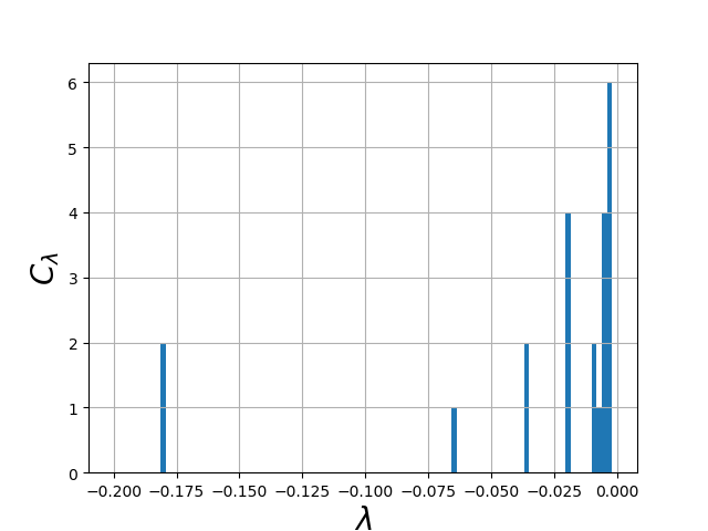
Figure 1: Eigenvalue density of the partial transpose $\rho^{T_{2}}$ for 96 angular bins, plotted over $[-0.2,0.0)$. To suppress the $\delta(\lambda)$ peak the eigenvalue multiplicity in the first bin left of 0 is not shown.

The binned eigenvalue density of the partial transpose $\rho^{T_{2}}$ also converges to the form of eq. (17), where now some of the $\lambda_{i}$ are negative. The multiplicities $C_{i}$ of negative eigenvalues are shown in fig. 1. We obtain ${\cal N}(\rho)\simeq 0.68$. This quantifies the magnitude of two-quark azimuthal quantum correlations encoded in the model wave function (12), when all other degrees of freedom have been traced over. Contrary to the state in color space described in sec. II, where the entropy is substantially greater than the negativity (even for ${N_{\mathrm{c}}}=3$ colors), here the entropy of the angular density matrix is actually less than its negativity. The coherent information measure described above confirms the presence of genuine quantum correlations: for the angular density matrix we obtain positive $I(2\rangle 1)=0.32$. When $\rho_{\phi_{1}\phi_{2},\phi_{1}^{\prime}\phi_{2}^{\prime}}$ is subjected to “classicalization” via the PEN transformation described in appendix B, coherent information turns negative: $I^{\prime}(2\rangle 1)=-1.04$.

To illustrate the potential relevance of entanglement negativity to concrete observables we have computed the following azimuthal angular moments of quark pairs in the proton:

$$a_{n}\equiv\left<e^{in(\phi_{1}-\phi_{2})}\right>=\int{\rm d}\phi_{1}{\rm d}\phi_{2}\,\rho_{\phi_{1}\phi_{2},\phi_{1}\phi_{2}}\,e^{in(\phi_{1}-\phi_{2})}$$ (18)

for $n=1,2,3$. As the diagonal of the density matrix is symmetric under $\phi_{1}\leftrightarrow\phi_{2}$ it follows that the imaginary parts of the above moments vanish. Table 1 lists the values of $a_{1},a_{2},a_{3}$ obtained with the three quark density matrix from eq. (13) as well as with the modified $\rho^{\prime}$ with vanishing entanglement negativity; see appendix B for a discussion of the transformation $\rho\to\rho^{\prime}$.

$n$	$a_{n}$	$a_{n}^{\prime}$
1	$-0.404$	$-0.121$
2	$0.152$	$0.046$
3	$-0.058$	$-0.017$

Table 1: Angular moments $a_{n}=\left<e^{in(\phi_{1}-\phi_{2})}\right>$ computed from the three quark density matrix. The primed moments correspond to the modified density matrix $\rho^{\prime}$ where quantum correlations associated with a negative eigenvalue of the partial transpose have been purged.

We find substantial changes of the $a_{n}$ when the entanglement negativity of the density matrix is erased. This is an indication that quantum correlations intrinsic to the proton could be relevant for the understanding of two-particle angular correlations in proton-nucleus collisions (see refs.[43, 44, 45] and references therein) or deeply inelastic scattering (see below), at least in the regime of moderately small $x$.

IV Summary and Discussion

In sec. II we consider the state of ${N_{\mathrm{c}}}$ quarks in color space. Tracing over the colors of ${N_{\mathrm{c}}}-2$ quarks generates a mixed state $\rho$ where the von Neumann entropy $S(\rho)=\log\frac{1}{2}{N_{\mathrm{c}}}({N_{\mathrm{c}}}-1)=2\log{N_{\mathrm{c}}}-\log 2-1/{N_{\mathrm{c}}}+\cdots$ is much greater than the level of quantum correlations measured by the entanglement negativity, ${\cal N}(\rho)=1/{N_{\mathrm{c}}}$.

In sec. III we turn to our main focus, two-quark azimuthal correlations in the proton on the light-front. We consider moderate-energy scattering which probes parton fractional momenta $x\,\,\vbox{\hbox{$\buildrel\displaystyle>\over{\sim}$}}\,\,0.1$, and transverse momenta not far beyond the QCD confinement scale. In this regime, an effective description of the proton in terms of a light-front constituent quark model should apply. Tracing out all other degrees of freedom, we construct the reduced density matrix $\rho_{\phi_{1}\phi_{2},\phi_{1}^{\prime}\phi_{2}^{\prime}}$ which describes angular correlations. Using a standard light-cone model wave function from the literature [38, 34] we make a novel observation, that this state is characterized by low entropy, $S\simeq 0.25$, and high entanglement negativity ${\cal N}\simeq 0.68$. This is indicative of the presence of strong quantum correlations among the two azimuthal angles, and of weaker entanglement of the combined system $(\phi_{1},\phi_{2})$ with the traced out “environment”. The reduced state of the quark pair corresponds to an entangled superposition of azimuths, not to a classical statistical ensemble. For illustration we have computed $\langle\exp(in(\phi_{1}-\phi_{2}))\rangle$ moments of quark pair angular correlations intrinsic to the proton from the three quark model light-cone wave function. We find that these angular correlation measures are clearly linked to the non-zero entanglement negativity of the density matrix, i.e. to the presence of negative eigenvalues of the partial transpose of $\rho$.

These azimuthal correlations could, in principle, be observed in deeply-inelastic $e^{-}p$ scattering at the electron-ion collider EIC [46, 47, 48, 49]. In this process, a small quark anti-quark dipole of transverse size $\vec{r}$ scatters from the proton at an impact parameter $\vec{b}$, and the scattering amplitude $N(\vec{r},\vec{b})$ depends on the azimuthal angle made by these two vectors.

Indeed, the angular dependence of

$$N(\vec{r},\vec{b})=-g^{4}C_{F}\int\frac{{\rm d}^{2}\vec{K}{\rm d}^{2}\vec{q}}{(2\pi)^{4}}\frac{\cos\left(\vec{b}\cdot\vec{K}\right)}{(\vec{q}-\frac{1}{2}\vec{K})^{2}\,\,(\vec{q}+\frac{1}{2}\vec{K})^{2}}\,\left(\cos(\vec{r}\cdot\vec{q})-\cos\left(\frac{\vec{r}\cdot\vec{K}}{2}\right)\!\!\right)\,G_{2}\left(\vec{q}-\frac{1}{2}\vec{K},-\vec{q}-\frac{1}{2}\vec{K}\right)~{},$$ (19)

is determined by the angular dependence of the correlator of two color charge density operators in the proton,

$$\langle Q^{a}(\vec{q}_{1})\,Q^{b}(\vec{q}_{2})\rangle\equiv\delta^{ab}\,g^{2}G_{2}(\vec{q}_{1},\vec{q}_{2})~{}.$$ (20)

Restricting to the three quark Fock state for illustration, the result for this correlator obtained in ref. [50] can be rewritten in terms of the density matrix $\rho_{\alpha\alpha^{\prime}}$ introduced above in eq. (13):

$$G_{2}(\vec{q}_{1},\vec{q}_{2}) = \int\frac{{\rm d}x_{1}\,{\rm d}x_{2}}{8x_{1}x_{2}(1-x_{1}-x_{2})}\int\frac{{\rm d}^{2}k_{1}\,{\rm d}^{2}k_{2}}{(16\pi^{3})^{2}}\left\{\rho_{k_{1}k_{2},k_{1}^{\prime}k_{2}^{\prime}}-\rho_{k_{1}k_{2},\ell_{1}\ell_{2}}\right\}~{},$$ (21)

where $\vec{k}_{1}^{\prime}=\vec{k}_{1}-(1-x_{1})(\vec{q}_{1}+\vec{q}_{2})$, $\vec{k}_{2}^{\prime}=\vec{k}_{2}+x_{2}(\vec{q}_{1}+\vec{q}_{2})$, $\vec{\ell}_{1}=\vec{k}_{1}-(1-x_{1})\vec{q}_{1}+x_{1}\vec{q}_{2}$, $\vec{\ell}_{2}=\vec{k}_{2}-(1-x_{2})\vec{q}_{2}+x_{2}\vec{q}_{1}$, and $k_{1}^{+}=k_{1}^{\prime+}=\ell_{1}^{+}=x_{1}P^{+}$, $k_{2}^{+}=k_{2}^{\prime+}=\ell_{2}^{+}=x_{2}P^{+}$. The first and second terms of eq. (21) originate from the “handbag” and “cat’s ears” diagrams, respectively. Note that this correlator satisfies a Ward identity and vanishes when either $\vec{q}_{1}$ or $\vec{q}_{2}\to 0$; this can be checked easily using the permutation symmetry of the wave function. Eqs. (19, 21) describe the scattering of the dipole from the entangled superposition state of the target.

The angular dependence of the correlator $G_{2}(\vec{q}_{1},\vec{q}_{2})$ and of the dipole scattering amplitude $N(\vec{r},\vec{b})$ has been analyzed in ref. [51], and was shown to be qualitatively different from “geometry based” models [52]. At smaller $x$, the angular dependence of $N(\vec{r},\vec{b})$ can, alternatively, be attributed to the elliptic gluon Wigner distribution [53]. The evolution of the azimuthal dependence of $N(\vec{r},\vec{b})$ with $x$, in the quasi-classical regime of very small $x$ has been analyzed in refs. [54, 55, 56].

In appendix C, we provide the expressions for the leading ${\cal O}(g^{2})$ perturbative correction to the density matrix for angular correlations. The additional presence (or the exchange) of a gluon in the proton leads to a much wider range of parton light-cone and transverse momenta. Here, $\rho^{(g^{2})}_{\phi_{1}\phi_{2},\phi_{1}^{\prime}\phi_{2}^{\prime}}$ is no longer a function only of the differences $\phi_{1}-\phi_{2}$ and $\phi_{1}^{\prime}-\phi_{2}^{\prime}$, and so the numerical cost of constructing the matrix increases by an order of magnitude. Nevertheless, to see how the perturbative correction affects the entropy and entanglement negativity of the quark pair density matrix we have performed a coarse numerical evaluation using 48 angular bins. We choose parameters so as to ensure that the perturbative correction remains reasonably small, i.e. $\alpha_{s}=0.1$, $\Delta^{2}=1$ GeV², $\Lambda^{2}=3$ GeV², and $\langle x_{q}\rangle/x=3$. Even so, we obtain $S(\rho^{(g^{2})})\simeq 0.88$, and ${\cal N}(\rho^{(g^{2})})\simeq 0.58$. Thus, as the longitudinal and transverse phase space for the perturbative gluon opens up, there is a substantial increase of the entropy and a slight drop of the negativity. We interpret this to indicate slightly weaker quark pair azimuthal quantum correlations, and stronger entanglement of the remaining azimuthal angles with the traced degrees of freedom.

Appendix A Separable vs. quantum correlated states

A product state is given by

$$\rho=\sigma_{1}\otimes\sigma_{2}~{}.$$ (22)

Here, $\sigma_{1},\sigma_{2}$ are density matrices for subsystems 1 and 2, respectively; these may be pure or mixed states. Such a state obviously describes uncorrelated subsystems. Also, the entropy is additive, $S(\rho)=S(\sigma_{1})+S(\sigma_{2})$.

Now consider

$$\rho=\sum_{i}p_{i}\,\,\rho^{(1)}_{i}\otimes\rho^{(2)}_{i}~{}.$$ (23)

This is a classical statistical mixture of product states (enumerated by the index $i$) each with a probability weight $p_{i}$, with $\sum_{i}p_{i}=1$. An example is given below for how such a state may result from a partial trace over an entangled pure state. Also, such states may be prepared through LOCC (local unitary operations and classical communication) from a product state $\rho\otimes\sigma$:

$$\rho\otimes\sigma\to\sum_{i}p_{i}\left(U_{i}\,\rho\,U^{\dagger}_{i}\right)\otimes\left(V_{i}\,\sigma\,V^{\dagger}_{i}\right)~{}.$$ (24)

In state (23), subsystems 1 and 2 do exhibit correlations: given an observable $O=O^{(1)}\otimes O^{(2)}$ we have

$$\,\mathrm{tr}\,O\rho=\sum_{i}p_{i}\,\,\,\mathrm{tr}\left(O^{(1)}\rho^{(1)}_{i}\right)\,\,\,\mathrm{tr}\left(O^{(2)}\rho^{(2)}_{i}\right) \neq \sum_{i}p_{i}\,\,\,\mathrm{tr}\left(O^{(1)}\rho^{(1)}_{i}\right)\,\,\sum_{j}p_{j}\,\,\,\mathrm{tr}\left(O^{(2)}\rho^{(2)}_{j}\right)$$ (26)

$$=\,\mathrm{tr}\,\left(O^{(1)}\rho^{(1)}\right)\,\,\mathrm{tr}\,\left(O^{(2)}\rho^{(2)}\right)~{}.$$

Here, $\rho^{(1)}=\,\mathrm{tr}_{2}\,\rho=\sum_{i}p_{i}\,\rho^{(1)}_{i}$ denotes the density matrix for subsystem 1, and $\rho^{(2)}$ that of subsystem 2. In referring to (23) as a classical mixture we do not imply that either sub-system is in a classical state. These may well be quantum states. However, we interpret the correlations as classical since they are determined by the classical probabilities $p_{i}$.

A mixed density matrix that can not be written in the form (23) is said to exhibit quantum correlations. Equivalently, $\langle O\rangle$ will not be given by a convex sum of products of expectation values in the respective subsystems, weighted by classical probabilities, like in eq. (26).

Deciding whether a state $\rho$ is separable is called the separability problem of Quantum Information Theory. It is believed to be NP-hard in general [57, 58]. One available measure for quantum correlations is the so-called negativity ${\cal N}(\rho)$ [28]. It is given by minus the sum of negative eigenvalues of the “partial transpose” of $\rho$ with respect to system 2 [59, 60]: $\rho^{T_{2}}=(I\otimes T)(\rho)$, where $I$ and $T$ denote the identity and transposition operators, respectively. Then,

$${\cal N}(\rho)=-\sum_{\lambda^{T_{2}}<0}\,\lambda^{T_{2}}~{}.$$ (27)

For a state like eq. (23) the negativity is zero since

$$\rho^{T_{2}}=\sum_{i}p_{i}\,\,\rho^{(1)}_{i}\otimes\rho^{(2)\,T}_{i}$$ (28)

has the same eigenvalues as $\rho$ itself, all of which are $\geq 0$. Hence, negativity is “blind” to classical correlations, unlike entanglement measures such as the von Neumann entropy, which measure both quantum and classical correlations. However, in high dimensional Hilbert spaces negativity may vanish even when the state does exhibit quantum correlations: ${\cal N}(\rho)=0$ is a necessary but not a sufficient criterion for a given density matrix to be a separable mixture like eq. (23). Nevertheless, if ${\cal N}(\rho)>0$ then $\rho$ is definitely not a sum of product states.

A simple example for the emergence of a classical mixture of product states from a partially traced pure state follows from a generalized GHZ state [61] of 3 or more qudits,

$$\rho^{\mathrm{GHZ}}=\frac{1}{d}\sum_{i,j}|i,i,i\rangle\,\langle j,j,j|~{}.$$ (29)

Here, $d$ is the dimension of the Hilbert space of each system. Tracing out one of the qudits leaves a separable mixed state of the form (23),

$$\,\mathrm{tr}_{3}\,\rho^{\mathrm{GHZ}}=\frac{1}{d}\sum_{n}|n,n\rangle\,\langle n,n|=\frac{1}{d}\sum_{n}|n\rangle\,\langle n|\,\otimes\,|n\rangle\,\langle n|~{}.$$ (30)

This density matrix has $d$ non-zero eigenvalues equal to $1/d$. Its entropy is $S=\log d$, and its negativity is ${\cal N}=0$. For $d\gg 1$ this is a high entropy classically correlated state without quantum correlations. As a result of the strong classical correlations the entropy is not proportional to the number of qudits left, i.e. it is not extensive.

Appendix B PEN: purging quantum correlations associated with non-zero negativity

Here we describe a transformation of a density matrix $\rho\to\rho^{\prime}$ such that the negativity ${\cal N}(\rho^{\prime})=0$, i.e. the partial transpose of $\rho^{\prime}$ does not have any negative eigenvalues. If $\rho$ represents a classical statistical mixture of product states as in eq. (23) then $\rho^{\prime}=\rho$. In other words, classical correlations associated with such a state are unaffected by the transformation. We reiterate that ${\cal N}(\rho)=0$ is a necessary but not a sufficient criterion for a given density matrix to be a separable mixture (except when the Peres-Horodecki criterion applies). Hence, while the transformation we describe next eliminates negative eigenvalues from the spectrum of the partial transpose, it does not necessarily generate a separable state of the form (23).

We obtain $\rho^{\prime}$ from the following sequence:

$$\rho\to\sigma=\rho^{T_{2}}\to\sigma_{D}=U^{\dagger}\sigma U\to\sigma_{D}^{\prime}=\Theta(\sigma_{D})\,\sigma_{D}\to\sigma^{\prime}=U\sigma_{D}^{\prime}U^{\dagger}\to\rho^{\prime}=\frac{(\sigma^{\prime})^{T_{2}}}{\mathrm{tr}\,\sigma^{\prime}}~{}.$$ (31)

That is, we diagonalize the partial transpose of $\rho$ through a unitary transformation $U$ of the basis. We then remove the negative eigenvalues of the partial transpose: $\Theta(A)$ denotes a matrix valued Heavyside function which returns a matrix with the same dimension as $A$ and with entries 0 or 1 if the corresponding entry of $A$ is $\leq 0$ or $>0$, respectively. We then undo the basis rotation and the partial transposition, and rescale $\rho^{\prime}$ so that $\mathrm{tr}\,\rho^{\prime}=1$. Note that $\rho^{\prime}$ is positive semi-definite and hermitian (if $\rho$ is), and so it represents a valid density matrix. Since $\rho^{\prime}\neq\rho$ if ${\cal N}(\rho)>0$, through this transformation one may study how subsystem correlations $\mathrm{tr}\,O^{(1)}\otimes O^{(2)}\,\rho$ are modified by the “Purge Entanglement Negativity” (PEN) transformation.

When $\sigma=\rho^{T_{2}}$ has one single negative eigenvalue $\lambda_{-}$, and a degenerate spectrum of $n-1$ positive eigenvalues $\lambda_{+}$ then the above transformation corresponds to shifting $\lambda_{-}$ up to 0, and shifting all positive eigenvalues down by $\lambda_{-}/(n-1)$. That is, in this case $\rho^{\prime}$ is obtained from $\rho$ by adding the following traceless matrix, in order to maintain normalization:

$$\rho^{\prime}=\rho+a(1\!\!1-n\rho)~{}.$$ (32)

The transformation (31) corresponds to choosing the minimal value for $a$ that leads to ${\cal N}(\rho^{\prime})=0$.

We now provide an explicit example for the color space density matrix given previously in eq. (3):

$$\rho_{ij,i^{\prime}j^{\prime}}=\frac{1}{{N_{\mathrm{c}}}({N_{\mathrm{c}}}-1)}\left(\delta_{ii^{\prime}}\delta_{jj^{\prime}}-\delta_{ij^{\prime}}\delta_{i^{\prime}j}\right)~{}.$$ (33)

From here onward we consider ${N_{\mathrm{c}}}\geq 3$ since ${\cal N}(\rho)=0$ for ${N_{\mathrm{c}}}=2$, so $\rho^{\prime}=\rho$ in that case.

The PEN transformation (31) results in

$$\rho^{\prime}=\frac{1}{{N_{\mathrm{c}}}({N_{\mathrm{c}}}+1)}\,1\!\!1+\frac{1}{{N_{\mathrm{c}}}+1}\,\rho~{}.$$ (34)

On the other hand, to determine the allowed values for $a$ from eq. (32) we first write the explicit form of the partial transpose of $\rho$ as a ${N_{\mathrm{c}}}^{2}\times{N_{\mathrm{c}}}^{2}$ matrix:

$$\sigma=\rho^{T_{2}}=\frac{1}{{N_{\mathrm{c}}}({N_{\mathrm{c}}}-1)}\begin{bmatrix}0\vspace{0.25em}&\overbrace{0\cdots 0}^{{N_{\mathrm{c}}}\rm\ times}&-1&\overbrace{0\cdots 0}^{{N_{\mathrm{c}}}\rm\ times}&-1&\cdots&-1&\overbrace{0\cdots 0}^{{N_{\mathrm{c}}}\rm\ times}&-1\\ \shortstack{0\vspace{-0.5em}\\ \vdots\\ 0}&\shortstack{\ \vspace{-0.5em}\\ I\\ {\color[rgb]{1,1,1} 0}}&\shortstack{0\vspace{-0.5em}\\ \vdots\\ 0}&\shortstack{\ \vspace{-0.5em}\\ 0\\ {\color[rgb]{1,1,1} 0}}&\shortstack{0\vspace{-0.5em}\\ \vdots\\ 0}&&\shortstack{0\vspace{-0.5em}\\ \vdots\\ 0}&\shortstack{\ \vspace{-0.5em}\\ 0\\ {\color[rgb]{1,1,1} 0}}&\shortstack{0\vspace{-0.5em}\\ \vdots\\ 0}\\ -1\vspace{0.25em}&0\cdots 0&0&0\cdots 0&-1&\cdots&-1&0\cdots 0&-1\\ \shortstack{0\vspace{-0.5em}\\ \vdots\\ 0}&\shortstack{\ \vspace{-0.5em}\\ 0\\ {\color[rgb]{1,1,1} 0}}&\shortstack{0\vspace{-0.5em}\\ \vdots\\ 0}&\shortstack{\ \vspace{-0.5em}\\ I\\ {\color[rgb]{1,1,1} 0}}&\shortstack{0\vspace{-0.5em}\\ \vdots\\ 0}&&\shortstack{0\vspace{-0.5em}\\ \vdots\\ 0}&\shortstack{\ \vspace{-0.5em}\\ 0\\ {\color[rgb]{1,1,1} 0}}&\shortstack{0\vspace{-0.5em}\\ \vdots\\ 0}\\ -1\vspace{0.25em}&0\cdots 0&-1&0\cdots 0&0&\cdots&-1&0\cdots 0&-1\\ \vdots\vspace{0.4em}&&\vdots&&\vdots&\ddots&\vdots&&\vdots\\ -1\vspace{0.4em}&0\cdots 0&-1&0\cdots 0&-1&\cdots&-1&0\cdots 0&0\\ \shortstack{0\vspace{-0.5em}\\ \vdots\\ 0}&\shortstack{\ \vspace{-0.5em}\\ 0\\ {\color[rgb]{1,1,1} 0}}&\shortstack{0\vspace{-0.5em}\\ \vdots\\ 0}&\shortstack{\ \vspace{-0.5em}\\ 0\\ {\color[rgb]{1,1,1} 0}}&\shortstack{0\vspace{-0.5em}\\ \vdots\\ 0}&&\shortstack{0\vspace{-0.5em}\\ \vdots\\ 0}&\shortstack{\ \vspace{-0.5em}\\ I\\ {\color[rgb]{1,1,1} 0}}&\shortstack{0\vspace{-0.5em}\\ \vdots\\ 0}\\ -1&0\cdots 0&-1&0\cdots 0&-1&\cdots&-1&0\cdots 0&0\end{bmatrix}\ .$$ (35)

The eigenspaces of $\sigma$ decouple since the ${N_{\mathrm{c}}}-1$ identity matrices have no overlap with the grid of $-1$s; trivially there are $({N_{\mathrm{c}}}-1){N_{\mathrm{c}}}$ eigenvectors with eigenvalue $[{N_{\mathrm{c}}}({N_{\mathrm{c}}}-1)]^{-1}$. Adding a diagonal matrix preserves the eigenspaces, so we can easily find the eigenvalues of $\sigma^{\prime}$ by taking the partial transpose of (32). The identity blocks on the diagonal of (35) are all multiplied by $(1-a{N_{\mathrm{c}}}^{2})$, then adding $aI$ means that the new eigenvalues are

$$a+(1-a{N_{\mathrm{c}}}^{2})\cdot\frac{1}{{N_{\mathrm{c}}}({N_{\mathrm{c}}}-1)}=\frac{1}{{N_{\mathrm{c}}}-1}\left(\frac{1}{{N_{\mathrm{c}}}}-a\right)\ .$$ (36)

The remaining eigenvalues are the eigenvalues of the ${N_{\mathrm{c}}}$-by-${N_{\mathrm{c}}}$ matrix

$$\begin{bmatrix}a&y&y&&y\\ y&a&y&\cdots&y\\ y&y&a&&y\\ &\vdots&&\ddots&\vdots\\ y&y&y&\cdots&a\end{bmatrix}$$ (37)

where

$$y=(1-a{N_{\mathrm{c}}}^{2})\cdot\frac{-1}{{N_{\mathrm{c}}}({N_{\mathrm{c}}}-1)}=\frac{a{N_{\mathrm{c}}}^{2}-1}{{N_{\mathrm{c}}}({N_{\mathrm{c}}}-1)}\ .$$ (38)

One eigenvector of (37) is $\sum_{i}\hat{e}_{i}$ with eigenvalue $a+({N_{\mathrm{c}}}-1)y$. The remaining ${N_{\mathrm{c}}}-1$ eigenvectors are of the form $\hat{e}_{1}-\hat{e}_{i}$ (for all $i\neq 1$) and all have eigenvalue $a-y$, which when worked out is equal to (36). Therefore the eigenvalues of $\sigma^{\prime}$ in (32) are $\lambda_{1}$ with multiplicity ${N_{\mathrm{c}}}^{2}-1$ and $\lambda_{2}$ with multiplicity 1, where

$$\lambda_{1} =\frac{1}{{N_{\mathrm{c}}}-1}\left(\frac{1}{{N_{\mathrm{c}}}}-a\right)$$ (39)

$$\lambda_{2} =a({N_{\mathrm{c}}}+1)-\frac{1}{{N_{\mathrm{c}}}}~{}.$$ (40)

If both of these eigenvalues are to be non-negative as to make ${\cal N}(\rho^{\prime})=0$, we require

$$\frac{1}{{N_{\mathrm{c}}}({N_{\mathrm{c}}}+1)}\leq a\leq\frac{1}{{N_{\mathrm{c}}}}\ .$$ (41)

For the minimal $a=[{N_{\mathrm{c}}}({N_{\mathrm{c}}}+1)]^{-1}$, the spectrum of $\rho^{\prime}$ as given in eq. (34) is $\lambda=({N_{\mathrm{c}}}^{2}-1)^{-1}$ with multiplicity ${N_{\mathrm{c}}}^{2}-1$, and $\lambda=0$ with multiplicity 1. Hence, after removal of the negative eigenvalue of $\rho^{T_{2}}$ the entropy increases to

$$S(\rho^{\prime})=\log({N_{\mathrm{c}}}^{2}-1)=2\log{N_{\mathrm{c}}}-\frac{1}{{N_{\mathrm{c}}}^{2}}+\cdots$$ (42)

Comparing to eq. (7) for $S(\rho)$ we note that the minimal shift $\rho\to\rho^{\prime}$ has removed the two leading correlation contributions: $-\log 2$ from anti-symmetrization as well as the term $-1/{N_{\mathrm{c}}}$, which is (minus) the negativity. Some correlation contributions to the entropy at integer powers of ${N_{\mathrm{c}}}^{-2}$ are still present, however.

Appendix C ${\cal O}(g^{2})$ correction to the angular density matrix

In this section we list the leading ${\cal O}(g^{2})$ correction to the angular density matrix. The details of the calculation of the one gluon emission/exchange correction to the proton state $|P\rangle$ in light-cone perturbation theory have been published in refs. [27, 62]. Here, we restrict to quoting the resulting expressions for the angular density matrix.

The density matrix is now given by the original LO quark density matrix plus the ${\cal O}(g^{2})$ virtual correction(s), plus the four-particle (qqqg) density matrix traced over the gluon.

We will restrict to the limit where the light-cone momentum cutoff $x$ for the gluon is much less than typical quark light-cone momentum fractions. Although not strictly required this kinematic restriction greatly simplifies the following expressions.

The first virtual correction arises when a quark in $|P\rangle$ or $\langle P|$ exchanges a gluon with itself. This replaces $\Psi^{*}\Psi$ in eq. (13, 16) by

$$\Psi_{\mathrm{qqq}}^{*}(k_{1}^{\prime},k_{2}^{\prime})\,\Psi_{\mathrm{qqq}}(k_{1},k_{2})\,\left[1-3\,C_{q}(\langle x_{q}\rangle;\,x,{\Lambda}/{\Delta})\right]$$ (43)

where

$$C_{q}(\langle x_{q}\rangle;\,x,\Lambda/\Delta) = 4g^{2}C_{F}\int\limits_{x}^{\langle x_{q}\rangle}\frac{{\rm d}x_{g}}{x_{g}}\frac{{\rm d}^{2}k_{g}}{16\pi^{3}}\,\left[\frac{1}{k_{g}^{2}+\Delta^{2}}-\frac{1}{k_{g}^{2}+\Lambda^{2}}\right]$$ (44)

$$= \frac{4g^{2}C_{F}}{16\pi^{2}}\,\log\frac{\langle x_{q}\rangle}{x}\,\log\frac{\Lambda^{2}}{\Delta^{2}}~{}.$$ (45)

Here, $C_{F}=4/3$ is the eigenvalue of the quadratic Casimir in the fundamental representation of color-$SU(3)$, and $\Delta$ and $\Lambda$ denote a collinear regulator and a UV subtraction point, respectively. For simplicity, here we take both to be constants, independent of $x_{g}$.

The second virtual correction is due to the exchange of a gluon by two quarks in $|P\rangle$ or $\langle P|$. When quarks 1 and 2 in $|P\rangle$ exchange a gluon,

$$\rho^{(12)}_{\alpha\alpha^{\prime}} = \frac{2g^{2}C_{F}N_{c}}{3}\int_{x}\frac{{\rm d}x_{g}}{x_{g}}\frac{{\rm d}^{2}k_{g}}{16\pi^{3}}\frac{1}{k_{g}^{2}+\Delta^{2}}\,\Psi^{*}(k_{1}^{\prime},k_{2}^{\prime})\,\Psi(k_{1}+k_{g},k_{2}-k_{g})~{}.$$ (46)

We add this to eq. (43). In fact, we need to also add the virtual corrections from gluon exchanges by other quarks, so we replace $\Psi^{*}(k_{1}^{\prime},k_{2}^{\prime})\,\Psi(k_{1}+k_{g},k_{2}-k_{g})$ in the previous expression by

$$\Psi^{*}(k_{1}^{\prime},k_{2}^{\prime})\,\Psi(k_{1}+k_{g},k_{2}-k_{g})+\Psi^{*}(k_{1}^{\prime},k_{2}^{\prime})\,\Psi(k_{1}+k_{g},k_{2})+\Psi^{*}(k_{1}^{\prime},k_{2}^{\prime})\,\Psi(k_{1},k_{2}+k_{g})$$ (47)

$$+ \Psi^{*}(k_{1}^{\prime}+k_{g},k_{2}^{\prime}-k_{g})\,\Psi(k_{1},k_{2})+\Psi^{*}(k_{1}^{\prime}+k_{g},k_{2}^{\prime})\,\Psi(k_{1},k_{2})+\Psi^{*}(k_{1}^{\prime},k_{2}^{\prime}+k_{g})\,\Psi(k_{1},k_{2})~{}.$$

We continue with the real emissions. Consider first the case where a gluon is emitted from quark 1 in $|P\rangle$ and quark 1’ in $\langle P|$. Eq. (51) of ref. [27] leads to the following expression for the four-particle qqqg state:

$$\rho_{\alpha\alpha^{\prime}}^{(11^{\prime})}=\frac{4g^{2}C_{F}N_{c}}{3}\,\Psi^{*}(k_{1}^{\prime},k_{2}^{\prime})\,\Psi(k_{1},k_{2})\,\frac{\vec{k}_{g}\cdot\vec{k}_{g}^{\prime}}{(k_{g}^{2}+\Delta^{2})\,(k_{g}^{\prime 2}+\Delta^{2})}~{}.$$ (48)

The trace over quark and gluon colors has already been performed, and the limit $x_{g}\ll x_{1}$, $x_{g}^{\prime}\ll x_{1}^{\prime}$ has been taken. The matrix indices are $\alpha=\{x_{1},\vec{k}_{1},x_{2},\vec{k}_{2},x_{g},\vec{k}_{g}\}$ and $\alpha^{\prime}=\{x_{1},\vec{k}_{1}^{\prime},x_{2},\vec{k}_{2}^{\prime},x_{g}^{\prime},\vec{k}_{g}^{\prime}\}$.

Here we have to mind a subtlety: the above density matrix was obtained by projecting $|P\rangle$ onto $\langle\alpha|=\langle k_{1}-k_{g};k_{2};k_{3}|$ and $\langle P|$ onto $|\alpha^{\prime}\rangle=|k_{1}^{\prime}-k_{g}^{\prime};k_{2}^{\prime};k_{3}^{\prime}\rangle$, with $\sum\vec{k}_{i}=\sum\vec{k}_{i}^{\prime}=0$. When we trace over the gluon we want to keep the quark momenta fixed, however. Hence, we need to first shift $k_{1}\to k_{1}+k_{g}$ and $k_{1}^{\prime}\to k_{1}^{\prime}+k_{g}^{\prime}$, and only then do we trace over $k_{g}$. This leads to

$$\rho_{\alpha\alpha^{\prime}}^{(11^{\prime})}=\frac{4g^{2}C_{F}N_{c}}{3}\,\int\frac{{\rm d}x_{g}}{x_{g}}\frac{{\rm d}^{2}k_{g}}{16\pi^{3}}\Psi^{*}(k_{1}^{\prime}+k_{g},k_{2}^{\prime})\,\Psi(k_{1}+k_{g},k_{2})\,\left[\frac{1}{k_{g}^{2}+\Delta^{2}}-\frac{1}{k_{g}^{2}+\Lambda^{2}}\right]~{}.$$ (49)

Here the UV subtraction has been included so that the trace is finite. Now the matrix indices are $\alpha=\{x_{1},\vec{k}_{1},x_{2},\vec{k}_{2}\}$ and $\alpha^{\prime}=\{x_{1},\vec{k}_{1}^{\prime},x_{2},\vec{k}_{2}^{\prime}\}$. The sums over the transverse momentum arguments of the wave functions are still 0, so $\Psi^{*}$, $\Psi$ are evaluated for $\vec{k}_{3}^{\prime}=-(\vec{k}_{1}^{\prime}+\vec{k}_{2}^{\prime}+\vec{k}_{g})$ and $\vec{k}_{3}=-(\vec{k}_{1}+\vec{k}_{2}+\vec{k}_{g})$, respectively. On the other hand, $x_{3}$ and $x_{3}^{\prime}$ are still given by $1-x_{1}-x_{2}$ and $1-x_{1}^{\prime}-x_{2}^{\prime}$, respectively, because we assumed that the integral is dominated by negligibly small $x_{g}$. This expression, plus analogous contributions which account for gluon emissions from 2, 2’ and 3, 3’, now have to be added to the integrand of eq. (13).
(Cross check: if we trace over quarks with the measure (14) then we can shift $k_{1}$ back, and once we multiply by 3 to also account for gluon emissions from 2, 2’ and 3, 3’, then we reproduce eq. (71) of ref. [27]. Furthermore, this contribution then cancels exactly against the ${\cal O}(g^{2})$ correction from eq. (43), as it should to preserve the trace of the density matrix.)

The second real emission correction is due to two different quarks in $|P\rangle$ and $\langle P|$ each emitting a gluon. Eq. (56) of [27], traced over quark colors, gives the four particle state

$$\rho_{\alpha\alpha^{\prime}}^{(12^{\prime})}=-\frac{2g^{2}C_{F}N_{c}}{3}\,\Psi^{*}(k_{1}^{\prime},k_{2}^{\prime})\,\Psi(k_{1},k_{2})\,\frac{\vec{k}_{g}\cdot\vec{k}_{g}^{\prime}}{(k_{g}^{2}+\Delta^{2})\,(k_{g}^{\prime 2}+\Delta^{2})}~{}.$$ (50)

Here we need to shift $k_{1}\to k_{1}+k_{g}$ and $k_{2}^{\prime}\to k_{2}^{\prime}+k_{g}^{\prime}$, and then we can trace out the gluon:

$$\rho_{\alpha\alpha^{\prime}}^{(12^{\prime})}=-\frac{2g^{2}C_{F}N_{c}}{3}\,\int\frac{{\rm d}x_{g}}{x_{g}}\frac{{\rm d}^{2}k_{g}}{16\pi^{3}}\Psi^{*}(k_{1}^{\prime},k_{2}^{\prime}+k_{g})\,\Psi(k_{1}+k_{g},k_{2})\,\frac{1}{k_{g}^{2}+\Delta^{2}}~{}.$$ (51)

Once again, here the transverse components of $k_{3},k_{3}^{\prime}$ are such that the sum of transverse momenta is 0. If we trace out the quarks, too, then $k_{1}^{\prime}=k_{1}$ and $k_{2}^{\prime}=k_{2}$; we are then allowed to shift $k_{2}\to k_{2}-k_{g}$ and (51) cancels against (46) so that the proper normalization of the density matrix is preserved.

In summary, to account for the ${\cal O}(g^{2})$ perturbative correction, in eq. (16) for $\rho_{\phi_{1}\phi_{2},\phi_{1}^{\prime}\phi_{2}^{\prime}}$ one replaces the LO density matrix $\Psi^{*}()\,\Psi()$ by the sum of eqs. (43), (46,47), (49) plus analogous contributions for (11’) $\to$ (22’), (33’), and (51) plus analogous contributions for (12’) $\to$ (13’), (21’), (23’), (31’), (32’). As we have indicated, the perturbative correction cancels in the sum of eigenvalues of the density matrix, which is therefore independent of the perturbative coupling $g^{2}$, the gluon light-cone momentum cutoff $x$, the collinear regulator $\Delta$, and the UV regulator $\Lambda$. However, the spectrum of eigenvalues does depend on these quantities, and so does the entropy and the negativity of $\rho$.

References

- Schrödinger [1935] E. Schrödinger, Discussion of probability relations between separated systems, Mathematical Proceedings of the Cambridge Philosophical Society 31, 555 (1935).
- Schrödinger [1936] E. Schrödinger, Probability relations between separated systems, Mathematical Proceedings of the Cambridge Philosophical Society 32, 446 (1936).
- Einstein et al. [1935] A. Einstein, B. Podolsky, and N. Rosen, Can Quantum-Mechanical Description of Physical Reality Be Considered Complete ?, Phys. Rev. 47, 777 (1935).
- Kovner and Lublinsky [2015] A. Kovner and M. Lublinsky, Entanglement entropy and entropy production in the Color Glass Condensate framework, Phys. Rev. D 92, 034016 (2015), arXiv:1506.05394 [hep-ph] .
- Kovner et al. [2019] A. Kovner, M. Lublinsky, and M. Serino, Entanglement entropy, entropy production and time evolution in high energy QCD, Phys. Lett. B 792, 4 (2019), arXiv:1806.01089 [hep-ph] .
- Hagiwara et al. [2018] Y. Hagiwara, Y. Hatta, B.-W. Xiao, and F. Yuan, Classical and quantum entropy of parton distributions, Phys. Rev. D 97, 094029 (2018), arXiv:1801.00087 [hep-ph] .
- Kharzeev [2021] D. E. Kharzeev, Quantum information approach to high energy interactions, Phil. Trans. A. Math. Phys. Eng. Sci. 380, 20210063 (2021), arXiv:2108.08792 [hep-ph] .
- Kharzeev and Levin [2017] D. E. Kharzeev and E. M. Levin, Deep inelastic scattering as a probe of entanglement, Phys. Rev. D 95, 114008 (2017), arXiv:1702.03489 [hep-ph] .
- Beane and Ehlers [2019] S. R. Beane and P. Ehlers, Chiral symmetry breaking, entanglement, and the nucleon spin decomposition, Mod. Phys. Lett. A 35, 2050048 (2019), arXiv:1905.03295 [hep-ph] .
- Ehlers [2022] P. J. Ehlers, Entanglement between Valence and Sea Quarks in Hadrons of 1+1 Dimensional QCD, (2022), arXiv:2209.09867 [hep-ph] .
- Tu et al. [2020] Z. Tu, D. E. Kharzeev, and T. Ullrich, Einstein-Podolsky-Rosen Paradox and Quantum Entanglement at Subnucleonic Scales, Phys. Rev. Lett. 124, 062001 (2020), arXiv:1904.11974 [hep-ph] .
- Kharzeev and Levin [2021] D. E. Kharzeev and E. Levin, Deep inelastic scattering as a probe of entanglement: Confronting experimental data, Phys. Rev. D 104, L031503 (2021), arXiv:2102.09773 [hep-ph] .
- Ramos and Machado [2020] G. S. Ramos and M. V. T. Machado, Investigating entanglement entropy at small- in DIS off protons and nuclei, Phys. Rev. D 101, 074040 (2020), arXiv:2003.05008 [hep-ph] .
- Hentschinski and Kutak [2022] M. Hentschinski and K. Kutak, Evidence for the maximally entangled low x proton in Deep Inelastic Scattering from H1 data, Eur. Phys. J. C 82, 111 (2022), arXiv:2110.06156 [hep-ph] .
- Hentschinski et al. [2022] M. Hentschinski, K. Kutak, and R. Straka, Maximally entangled proton and charged hadron multiplicity in Deep Inelastic Scattering, Eur. Phys. J. C 82, 1147 (2022), arXiv:2207.09430 [hep-ph] .
- Zhang et al. [2022] K. Zhang, K. Hao, D. Kharzeev, and V. Korepin, Entanglement entropy production in deep inelastic scattering, Phys. Rev. D 105, 014002 (2022), arXiv:2110.04881 [quant-ph] .
- Andreev et al. [2021] V. Andreev et al. (H1), Measurement of charged particle multiplicity distributions in DIS at HERA and its implication to entanglement entropy of partons, Eur. Phys. J. C 81, 212 (2021), arXiv:2011.01812 [hep-ex] .
- Armesto et al. [2019] N. Armesto, F. Dominguez, A. Kovner, M. Lublinsky, and V. Skokov, The Color Glass Condensate density matrix: Lindblad evolution, entanglement entropy and Wigner functional, JHEP 05, 025, arXiv:1901.08080 [hep-ph] .
- Duan et al. [2020] H. Duan, C. Akkaya, A. Kovner, and V. V. Skokov, Entanglement, partial set of measurements, and diagonality of the density matrix in the parton model, Phys. Rev. D 101, 036017 (2020), arXiv:2001.01726 [hep-ph] .
- Duan et al. [2022] H. Duan, A. Kovner, and V. V. Skokov, Gluon quasiparticles and the CGC density matrix, Phys. Rev. D 105, 056009 (2022), arXiv:2111.06475 [hep-ph] .
- Duan et al. [2023] H. Duan, A. Kovner, and V. V. Skokov, Classical Entanglement and Entropy, (2023), arXiv:2301.05735 [quant-ph] .
- Dvali and Venugopalan [2022] G. Dvali and R. Venugopalan, Classicalization and unitarization of wee partons in QCD and gravity: The CGC-black hole correspondence, Phys. Rev. D 105, 056026 (2022), arXiv:2106.11989 [hep-th] .
- Liu et al. [2022a] Y. Liu, M. A. Nowak, and I. Zahed, Rapidity evolution of the entanglement entropy in quarkonium: Parton and string duality, Phys. Rev. D 105, 114028 (2022a), arXiv:2203.00739 [hep-ph] .
- Liu et al. [2022b] Y. Liu, M. A. Nowak, and I. Zahed, Mueller’s dipole wave function in QCD: emergent KNO scaling in the double logarithm limit, (2022b), arXiv:2211.05169 [hep-ph] .
- Asadi and Vaidya [2022] P. Asadi and V. Vaidya, Quantum Entanglement and the Thermal Hadron, (2022), arXiv:2211.14333 [nucl-th] .
- Asadi and Vaidya [2023] P. Asadi and V. Vaidya, 1+1D Hadrons Minimize their Biparton Renyi Free Energy, (2023), arXiv:2301.03611 [hep-th] .
- Dumitru and Kolbusz [2022] A. Dumitru and E. Kolbusz, Quark and gluon entanglement in the proton on the light cone at intermediate , Phys. Rev. D 105, 074030 (2022), arXiv:2202.01803 [hep-ph] .
- Vidal and Werner [2002] G. Vidal and R. F. Werner, Computable measure of entanglement, Phys. Rev. A 65, 032314 (2002), arXiv:quant-ph/0102117 [hep-ph] .
- Plenio [2005] M. B. Plenio, Logarithmic Negativity: A Full Entanglement Monotone That is not Convex, Phys. Rev. Lett. 95, 090503 (2005).
- Wilde [2011] M. M. Wilde, From Classical to Quantum Shannon Theory (2011) arXiv:1106.1445 .
- Lepage and Brodsky [1980] G. Lepage and S. J. Brodsky, Exclusive Processes in Perturbative Quantum Chromodynamics, Phys. Rev. D 22, 2157 (1980).
- Brodsky et al. [1998] S. J. Brodsky, H.-C. Pauli, and S. S. Pinsky, Quantum chromodynamics and other field theories on the light cone, Phys. Rept. 301, 299 (1998), arXiv:hep-ph/9705477 .
- Brodsky et al. [2001] S. J. Brodsky, D. S. Hwang, B.-Q. Ma, and I. Schmidt, Light cone representation of the spin and orbital angular momentum of relativistic composite systems, Nucl. Phys. B 593, 311 (2001), arXiv:hep-th/0003082 .
- Brodsky and Schlumpf [1994] S. J. Brodsky and F. Schlumpf, Wave function independent relations between the nucleon axial coupling and the nucleon magnetic moments, Phys. Lett. B 329, 111 (1994), arXiv:hep-ph/9402214 .
- Ji et al. [2021] X. Ji, Y.-S. Liu, Y. Liu, J.-H. Zhang, and Y. Zhao, Large-momentum effective theory, Rev. Mod. Phys. 93, 035005 (2021), arXiv:2004.03543 [hep-ph] .
- Ji and Liu [2022] X. Ji and Y. Liu, Computing light-front wave functions without light-front quantization: A large-momentum effective theory approach, Phys. Rev. D 105, 076014 (2022), arXiv:2106.05310 [hep-ph] .
- Liu et al. [2021] Y. Liu, Y. Zhao, and A. Schäfer, Light-front wavefunction from lattice QCD through large-momentum effective theory, https://www.snowmass21.org/docs/files/summaries/TF/SNOWMASS21-TF2_TF5-CompF2_CompF0-044.pdf (2021), [Online; accessed 19-December-2021].
- Schlumpf [1993] F. Schlumpf, Relativistic constituent quark model of electroweak properties of baryons, Phys. Rev. D 47, 4114 (1993), [Erratum: Phys.Rev.D 49, 6246 (1994)], arXiv:hep-ph/9212250 .
- Xu et al. [2021] S. Xu, C. Mondal, J. Lan, X. Zhao, Y. Li, and J. P. Vary (BLFQ), Nucleon structure from basis light-front quantization, Phys. Rev. D 104, 094036 (2021), arXiv:2108.03909 [hep-ph] .
- Shuryak and Zahed [2022] E. Shuryak and I. Zahed, Hadronic structure on the light-front IV: Heavy and light Baryons, (2022), arXiv:2202.00167 [hep-ph] .
- Bakker et al. [1979] B. L. G. Bakker, L. A. Kondratyuk, and M. V. Terentev, On the formulation of two-body and three-body relativistic equations employing light front dynamics, Nucl. Phys. B 158, 497 (1979).
- Witten [1979] E. Witten, Baryons in the 1/n Expansion, Nucl. Phys. B 160, 57 (1979).
- Kohara et al. [2023] A. K. Kohara, C. Marquet, and V. Vila, Low projectile density contributions in the dilute-dense CGC framework for two-particle correlations, (2023), arXiv:2303.08711 [hep-ph] .
- Lappi et al. [2016] T. Lappi, B. Schenke, S. Schlichting, and R. Venugopalan, Tracing the origin of azimuthal gluon correlations in the color glass condensate, JHEP 01, 061, arXiv:1509.03499 [hep-ph] .
- Schenke et al. [2015] B. Schenke, S. Schlichting, and R. Venugopalan, Azimuthal anisotropies in pPb collisions from classical Yang–Mills dynamics, Phys. Lett. B 747, 76 (2015), arXiv:1502.01331 [hep-ph] .
- Accardi et al. [2016] A. Accardi et al., Electron Ion Collider: The Next QCD Frontier: Understanding the glue that binds us all, Eur. Phys. J. A 52, 268 (2016), arXiv:1212.1701 [nucl-ex] .
- Aschenauer et al. [2019] E. C. Aschenauer, S. Fazio, J. H. Lee, H. Mäntysaari, B. S. Page, B. Schenke, T. Ullrich, R. Venugopalan, and P. Zurita, The electron–ion collider: assessing the energy dependence of key measurements, Rept. Prog. Phys. 82, 024301 (2019), arXiv:1708.01527 [nucl-ex] .
- Pro [2020] Proceedings, Probing Nucleons and Nuclei in High Energy Collisions: Dedicated to the Physics of the Electron Ion Collider: Seattle (WA), United States, October 1 - November 16, 2018 (WSP, 2020) arXiv:2002.12333 [hep-ph] .
- Abdul Khalek et al. [2022] R. Abdul Khalek et al., Science Requirements and Detector Concepts for the Electron-Ion Collider: EIC Yellow Report, Nucl. Phys. A 1026, 122447 (2022), arXiv:2103.05419 [physics.ins-det] .
- Dumitru et al. [2018] A. Dumitru, G. A. Miller, and R. Venugopalan, Extracting many-body color charge correlators in the proton from exclusive DIS at large Bjorken x, Phys. Rev. D 98, 094004 (2018), arXiv:1808.02501 [hep-ph] .
- Dumitru et al. [2021] A. Dumitru, H. Mäntysaari, and R. Paatelainen, Color charge correlations in the proton at NLO: Beyond geometry based intuition, Phys. Lett. B 820, 136560 (2021), arXiv:2103.11682 [hep-ph] .
- Iancu and Rezaeian [2017] E. Iancu and A. H. Rezaeian, Elliptic flow from color-dipole orientation in pp and pA collisions, Phys. Rev. D 95, 094003 (2017), arXiv:1702.03943 [hep-ph] .
- Hagiwara et al. [2017] Y. Hagiwara, Y. Hatta, B.-W. Xiao, and F. Yuan, Elliptic Flow in Small Systems due to Elliptic Gluon Distributions?, Phys. Lett. B 771, 374 (2017), arXiv:1701.04254 [hep-ph] .
- Kovner and Lublinsky [2011a] A. Kovner and M. Lublinsky, Angular Correlations in Gluon Production at High Energy, Phys. Rev. D 83, 034017 (2011a), arXiv:1012.3398 [hep-ph] .
- Kovner and Lublinsky [2011b] A. Kovner and M. Lublinsky, On Angular Correlations and High Energy Evolution, Phys. Rev. D 84, 094011 (2011b), arXiv:1109.0347 [hep-ph] .
- Dumitru and Skokov [2015] A. Dumitru and V. Skokov, Anisotropy of the semiclassical gluon field of a large nucleus at high energy, Phys. Rev. D 91, 074006 (2015), arXiv:1411.6630 [hep-ph] .
- Gurvits [2002] L. Gurvits, Quantum matching theory (with new complexity theoretic, combinatorial and topological insights on the nature of the quantum entanglement), arXiv preprint quant-ph/0201022 (2002).
- Horodecki et al. [2009] R. Horodecki, P. Horodecki, M. Horodecki, and K. Horodecki, Quantum entanglement, Rev. Mod. Phys. 81, 865 (2009), arXiv:quant-ph/0702225 [quant-ph] .
- Peres [1996] A. Peres, Separability Criterion for Density Matrices, Phys. Rev. Lett. 77, 1413 (1996), arXiv:quant-ph/9604005 [quant-ph] .
- Horodecki et al. [1996] M. Horodecki, P. Horodecki, and R. Horodecki, Separability of mixed states: necessary and sufficient conditions, Phys. Lett. A 233, 1 (1996), arXiv:quant-ph/9605038 [quant-ph] .
- Greenberger et al. [2007] D. M. Greenberger, M. A. Horne, and A. Zeilinger, Going Beyond Bell’s Theorem 10.48550/arXiv.0712.0921 (2007), arXiv:0712.0921 [quant-ph] .
- Dumitru and Paatelainen [2021] A. Dumitru and R. Paatelainen, Sub-femtometer scale color charge fluctuations in a proton made of three quarks and a gluon, Phys. Rev. D 103, 034026 (2021), arXiv:2010.11245 [hep-ph] .