Enhancing LiDAR performance: Robust De-skewing Exclusively Relying on Range Measurements

Abstract

Most commercially available Light Detection and Ranging (LiDAR)s measure the distances along a 2D section of the environment by sequentially sampling the free range along directions centered at the sensor’s origin. When the sensor moves during the acquisition, the measured ranges are affected by a phenomenon known as "skewing", which appears as a distortion in the acquired scan. Skewing potentially affects all systems that rely on LiDAR data, however, it could be compensated if the position of the sensor were known each time a single range is measured. Most methods to de-skew a LiDAR are based on external sensors such as IMU or wheel odometry, to estimate these intermediate LiDAR positions. In this paper, we present a method that relies exclusively on range measurements to effectively estimate the robot velocities which are then used for de-skewing. Our approach is suitable for low-frequency LiDAR where the skewing is more evident. It can be seamlessly integrated into existing pipelines, enhancing their performance at a negligible computational cost.

I Introduction

Accurate and reliable mapping, localization, and navigation are essential for a wide range of robotics applications from autonomous driving, logistics, search and rescue, and many others. To this extent, Light Detection and Ranging (LiDAR) sensors are a popular choice since they allow us to sense both the free space and the location of obstacles around the robot. A planar LiDAR measures the distance of an object by deflecting laser beams around the sensor’s axis of rotation.

(a)

(b)

(c)

Figure 1: Effect of de-skewing. (a) Unprocessed (raw) scan acquired by a rotating robot, while (b) is the corresponding ground truth scan, and finally (c) is the same scan in (a), processed (de-skewed) using our proposed approach.

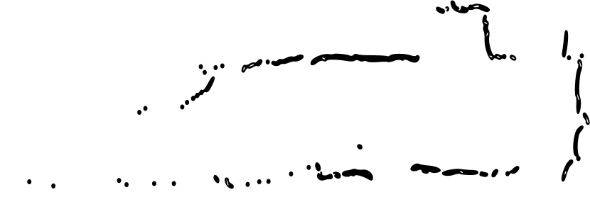
In this work we focus on low-grade 2D LiDAR s such as the InnoMaker-LD-06 or the RPI-Lidar A1 which at the time of writing can be bought for less than 100 Eur. The major shortcoming of these devices is their relatively slow angular speed which results in a full sweep of measurements becoming available at a frequency between 5 to 10 Hz. In contrast to more expensive models, these devices are not equipped with an inertial measurement unit or other means to estimate the proprioceptive motion of the sensor while it moves. In such devices, the scan acquisition(a full sweep of laser beams around the vertical axis of the sensor) is not instantaneous, hence when the robot carrying the LiDAR moves, the origin of the beam in the world frame changes for each sensed range. Neglecting this fact, and assuming that all measurements gathered during one rotation are sampled at the same time resulting in a distorted or skewed scan as shown in Fig. 1. Despite this consideration, most perception subsystems in a navigation stack treat the scans as rigid bodies, however, the effect of skewing leads to undesirable decay in accuracy that can result in failures as analyzed by Al-Nuaimi et al. [1].

A common way to compensate for the motion of the LiDAR is to integrate external proprioceptive measurements (dead reckoning and/or Inertial Measurement Unit (IMU)), to estimate the origin and orientation of the laser beam each time a range is acquired [4, 13, 7]. High-end 3D LiDAR s already contain a synchronized IMU, which is not available on the inexpensive models previously mentioned.

In this paper, we propose an approach to estimate the velocities of the robot carrying the LiDAR, based solely on the range measurements, that are processed as a stream. Our method is based on a non-rigid plane-to-plane registration algorithm, where the velocity of the platform carrying the sensor is estimated by maximizing the geometric consistency of the stream of ranges. We conducted several statistical experiments on synthetic and real data. Results verify that our de-skewing method is effective in estimating the motion of the robot, at negligible computation.

In Fig. 1 we illustrate the effects of our approach on measurements acquired with a constantly rotating LiDAR, with a rotational velocity 3 rad/s. In the remainder of this paper, we first review the related work in Sec. II, subsequently we describe in detail our de-skewing method for 2D LiDAR data Sec. III. We conclude the paper by presenting some synthetic and real results in Sec. IV, that show the ability of the proposed system. And finally, we draw some conclusions on the benefits and the limitations of our approach.

II Related Work

In this section, we review the most recent approaches to de-skew LiDAR data. Existing approaches for de-skewing mostly use either wheeled odometry or IMU to estimate the relative motion of the sensor/robot while a scan is being acquired. This process involves motion integration relying on estimators that process the raw proprioceptive data such as a filter or an integrator that directly provides an estimate of the sensor position each time a single range is measured.

These methods fall in the class of loosely-coupled, since they do not use the LiDAR information to refine the proprioceptive estimate. Among this class, we find the work of Tang et al. [9] that proposes to match subsequent scans to compute the relative motion, where the initial relative orientations are provided by an IMU. Subsequently, He et al. [4] proposed a method to estimate relative motion between IMU poses and de-skew subsequent ranges by using these smoothed poses.

In contrast to loosely-coupled approaches, tightly-coupled methods jointly process LiDAR and IMU. These methods are typically based on either smoothing or filtering. Wei  et al. [11] uses a pre-integration scheme to estimate the LiDAR’s ego-motion based on the inertial measurements, and updates the IMU biases in the correct step of an iterative EKF whenever a scan is completed. Shan  et al. [8] includes the states of IMU in the factor-graph, updating IMU biases through the optimization process, adapting a well-known computer vision work [3] to the LiDAR case. These ideas have been further extended in [10, 12] where the authors resort to full factor-graph optimization to obtain a state configuration that is maximally consistent with all the IMU measurements and LiDAR ranges.

For coupled approaches, accurate time synchronization between the sensors is essential. Unfortunately, this is not straightforward to obtain on inexpensive small devices due to the unpredicted communication latencies that affect the communication channels. These issues, however, can be completely avoided when using only LiDAR data to perform de-skewing. At their core LiDAR only methods have a registration algorithm, which aims to compute the velocities of the sensor while the robot moves. The basic intuition is that if the correct velocities were found, the sequence of range measurements could be assembled in a maximally consistent scan. In this context, Moosman et al. [6] propose to linearly interpolate scans between the last known pose, and the currently estimated pose, de-skewing the scan at both poses. However, this double approximation might hinder the accuracy when the initial registration fails, resulting in even worse estimates.

Al-Nuaimi et al. [1] propose a weighting schema based on their adapted Geometric Algebra LMS solver, where they assume that consecutive relative translation and angular motion are equal, which might be inaccurate due to the existence of drift and friction.

In this paper, we propose a planar LiDAR-only approach that addresses the de-skewing problem by continuously registering the the sequence of range measurements. The registration is carried on by estimating the LiDAR’s planar velocity, which iteratively minimizes a plane-to-plane metric between the de-skewed endpoints. Our results demonstrate that our methodology is accurate in estimating the velocity of the robot, only based on the laser measurements.

III Our Approach

Our method leverages some mild assumptions about the motion of the sensor mounted on the robot and the structure of the environment to operate on a continuous stream of range measurements. More specifically we assume to have a 2D slow LiDAR sensor, hence, we define each measurement as $\mathbf{z}_{i}=\left<r_{i},\alpha_{i},t_{i}\right>$. Here, $r_{i}$ is the range, $\alpha_{i}$ is the angle of the laser beam with respect to the origin of the sensor and $t_{i}$ is the timestamp. We assume the environment consists of a locally smooth surface and that the robot velocities change mildly within a LiDAR beam revolution.

Our method estimates these velocities by registering the stream of measurements $\{\mathbf{z}_{i}\}$ onto itself. The most likely velocities are the ones that if applied for de-skewing renders the measurement maximally consistent. Consistency is measured by a plane-to-plane metric applied between the corresponding LiDAR endpoints. More formally, let $\mathbf{x}=\left(v\hskip 5.69046pt\omega\right)^{T}$ be the translational and angular velocity of the robot we want to estimate $\mathbf{x}^{*}$, such that

$$\mathbf{x}^{*}=\mathop{\rm argmin}_{\mathbf{x}}\sum_{\left<i,j\right>\in\mathcal{C}}\rho\lVert\mathbf{e}(\mathbf{x},t_{i},t_{j})\rVert^{2}.$$ (1)

Where $\mathbf{e}(\mathbf{x},t_{i},t_{j})$ denotes an error vector between two planar scan patches computed around two corresponding range measurements at the time $t_{i}$ and $t_{j}$. The optimization step estimates new velocities $\mathbf{x}=(v\;\omega)^{T}$ under the current set of correspondences $\mathcal{C}$, using Iterative Reweighted Least-Squares (IRLS). In Eq. (1) $\rho$ denotes the Huber robust estimator.

Our algorithm is an instance of Iterative Closest Point (ICP) since it proceeds by alternating between the data association and optimization steps. In the data association step, the corresponding endpoints are found using the nearest neighbor strategy based on current velocity estimates. In the optimization step, the velocities are refined from the new correspondences found by the data association.

III-A Velocity Based De-skewing

Whereas our approach can be applied to more complex kinematics, for the sake of simplicity we detail the common case of a unicycle mobile base. Our goal is to estimate the location $\mathbf{T}(\mathbf{x},t_{i})=\left(\begin{matrix}x_{i}&y_{i}&\theta_{i}\end{matrix}\right)^{T}$ of the mobile base at time $t_{i}$, assuming it starts from the origin and progresses with constant translation and angular velocities over sampling time $\mathbf{x}=(v\hskip 5.69046pt\omega)^{T}$. After a time $t_{i}$, the robot would have traveled for a distance $l_{i}=v\cdot t_{i}$ and its angle is $\theta_{i}=\omega\cdot t_{i}$. The base will move along an arc of radius $R$, such that:

$$R = \frac{v_{i}}{\omega_{i}}=\frac{l_{i}}{\theta_{i}}.$$ (2)

From this consideration, we can easily compute $\mathbf{T}$ as

$$\mathbf{T}(\mathbf{x},t_{i})=\left(\begin{array}[]{c}R\sin{\theta_{i}}\\ R(1-\cos{\theta_{i}})\end{array}\right)=\underbrace{v\cdot t_{i}}_{l_{i}}\left(\begin{array}[]{c}\frac{\sin{\theta_{i}}}{\theta_{i}}\\ \frac{1-\cos{\theta_{i}}}{\theta_{i}}\end{array}\right)$$ (7)

Assuming the sensor (LiDAR) is located at the center of the mobile base, if at time $t_{i}$ the beam has a relative angle $\alpha_{i}$ and reports a range measurement $r_{i}$, we can straightforwardly find the 2D laser endpoint $\mathbf{p}_{i}$ as follows:

$$\mathbf{p}_{i}(\mathbf{x},t_{i}) = \mathbf{R}(\theta_{i}+\alpha_{i}){\begin{pmatrix}r_{i}\\ 0\end{pmatrix}}+\begin{pmatrix}x_{i}\\ y_{i}\end{pmatrix}.$$ (8)

Here $\mathbf{R}(\theta_{i}+\alpha_{i})\in SO(2)$ is 2D rotation matrix of $\theta_{i}+\alpha_{i}$. Applying this process to all the measurements and mapping all reconstructed points back to the pose where the acquisition of the current scan was started, results in the desired de-skew operation.

III-B Error Metric

To evaluate a plane-to-plane distance the algorithm needs to compute the normal vectors, which are based on the endpoints. Since the position of the endpoints is a function of the estimated velocities $\mathbf{x}$, also the normal vectors are. Hence the algorithm has to recompute both endpoints and normals at each iteration. Furthermore, when subsequent endpoints are too close, the noise affecting the range might result in an unstable normal vector, which hinders the error metric. To lessen this effect, before each iteration, we regularize the scan to retain only temporally subsequent measurements that are sufficiently far from each other to ensure a stable normal. In our experiments, we set this threshold to 0.15 m. Similarly, if there is a large distance gap between two subsequent endpoints ($>$0.4 m), likely, the surface is not continuous at that point, hence we drop those measurements too. At the end of this regularization step, we end up with a set of reasonably stable measurements we can use for the remainder of the computation. For each temporally subsequent pair of endpoints, we compute a planar patch $\mathbf{m}_{i}=\left<\mathbf{c}_{i},\mathbf{n}_{i},t_{i}\right>$, characterized by a center $\mathbf{c}_{i}$, a normal vector $\mathbf{n}_{i}$, and a timestamp $t_{i}$, such that:

$$\mathbf{c}_{i} = \frac{1}{2}\left(\mathbf{p}_{i+k}+\mathbf{p}_{i}\right),$$ (9)

$$\mathbf{n}_{i} = \left(\begin{array}[]{cc}\hskip 2.84544pt0&1\\ -1&0\end{array}\right)\frac{\mathbf{p}_{i+k}-\mathbf{p}_{i}}{\lVert\mathbf{p}_{i+k}-\mathbf{p}_{i}\rVert},$$ (12)

$$t_{i} = \frac{1}{2}\left(t_{i+k}+t_{i}\right).$$ (13)

Here, the index $k>0$ accounts for endpoints suppressed during regularization. If two planar patches $\mathbf{m}_{i}$ and $\mathbf{m}_{j}$ corresponds to the same portion of the environment, we can calculate an error vector $\mathbf{e}(\mathbf{x},t_{i},t_{j})$ accounting for both their differences in position and orientation. The error vector is a function of the velocities, since the patches $\mathbf{m}_{i}$ and $\mathbf{m}_{j}$ are computed based on the endpoints. The latter is related to the velocities by Eq. (8).

Let $\mathbf{e}(\mathbf{x},t_{i},t_{j})\in\mathbb{R}^{3}$ be the error vector, whose components are defined as follows:

$$\mathbf{e}(\mathbf{x},t_{i},t_{j}) = \left(\begin{array}[]{cc}\frac{1}{2}(\mathbf{c}_{i}-\mathbf{c}_{j})^{T}(\mathbf{n}_{i}+\mathbf{n}_{j})\\ \mathbf{n}_{j}-\mathbf{n}_{i}\end{array}\right).$$ (16)

Here the first dimension accounts for the distance between two corresponding planar patches $\mathbf{m}_{i}$ and $\mathbf{m}_{j}$ projected along the average of their normals. The other two account for the difference between the normal vectors. Eq. (16) is differentiable in the velocities $\mathbf{x}$, hence we can minimize Eq. (1) by Iterative Reweighted Least Squares.

Figure 2: Illustration of the planar patches calculation and the correspondence search between two matching patches $\mathbf{m}_{i}$ and $\mathbf{m}_{j}$.

III-C Data Association

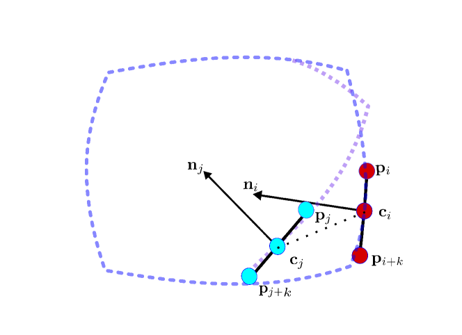
To determine the correspondence we proceed at each iteration by de-skewing the sequence of measurements, to get a set of updated endpoints $\mathbf{p}_{i}$. Subsequently, we apply the regularization to discard those measurements whose endpoints fall either too close or too far from their temporal neighbors. This gives us a set of sequential stable measurements we can use to extract the planar patches. Fig. 2 demonstarates the data association procedure.

Once this is done, for each $\mathbf{m}_{i}$ we seek for those other patches $\mathbf{m}_{j}$ that fulfill all the following criteria:

• their centers are close enough $\lvert\mathbf{c}_{i}-\mathbf{c}_{j}\rvert<\tau_{\mathbf{c}}$,

• their normals are sufficiently parallel $\mathbf{n}_{i}\cdot\mathbf{n}_{j}>\tau_{\mathbf{n}}$,

• their timestamp are sufficiently distant $\lvert t_{i}-t_{j}\rvert>\tau_{t}$.

Within this set we select as correspondence for $\mathbf{m}_{i}$, which is the $\mathbf{m}_{j}$ having the smallest projective distance $(\mathbf{c}_{i}-\mathbf{c}_{j})^{T}(\mathbf{n}_{i}+\mathbf{n}_{j})$.

Figure 3: Iterative evolution of the de-skewing process. Purple points represent skewed points, green points are the ground truth points, and blue lines represent the data association. Initial configuration, instance of full scan acquisition, with RMSE = 0.4 m. After 4 iterations of processing (de-skewing) the raw scan with the proposed approach, with decreased RMSE error to = 0.2 m. After 20 iterations, we ended up with a de-skewed scan closer to the ground truth, with RMSE = 0.074 m.

IV Experimental Validation

In this section, we present quantitative evaluations to demonstrate the accuracy of the velocities estimated by our approach, and its effect on the processed data, using only LiDAR measurements. To this extent, we carried out statistical experiments under changing velocities.

The goal of the first experiment is to compare the velocities of the robot calculated by our approach with the ground truth applied. As mentioned before utilizing the estimated velocities by our approach, renders measurements geometrically consistent as seen in Fig. 3.

	-2.000	-1.000	-0.500	0.500	1.000	2.000
-2.000	-1.936$\pm$0.090	-0.950$\pm$0.068	-0.471$\pm$0.050	0.470$\pm$0.047	0.962$\pm$0.052	1.910$\pm$0.092
	-1.952$\pm$0.081	-1.933$\pm$0.115	-1.958$\pm$0.066	-1.962$\pm$0.052	-1.952$\pm$0.070	-1.932$\pm$0.103
	$\mathbf{0.090}$$/$0.404	$\mathbf{0.083}$$/$0.399	$\mathbf{0.059}$$/$0.351	$\mathbf{0.061}$$/$0.414	$\mathbf{0.055}$$/$0.460	$\mathbf{0.081}$$/$0.579
-1.000	-1.890$\pm$0.131	-0.979$\pm$0.031	-0.477$\pm$0.035	0.482$\pm$0.034	0.946$\pm$0.069	1.897$\pm$0.073
	-0.949$\pm$0.069	-0.986$\pm$0.023	-0.973$\pm$0.037	-0.979$\pm$0.026	-0.953$\pm$0.059	-0.950$\pm$0.056
	$\mathbf{0.067}$$/$0.297	$\mathbf{0.058}$$/$0.308	$\mathbf{0.055}$$/$0.296	$\mathbf{0.049}$$/$0.354	$\mathbf{0.054}$$/$0.336	$\mathbf{0.062}$$/$0.399
-0.500	-1.929$\pm$0.085	-0.978$\pm$0.063	$-0.479\pm$0.054	0.492$\pm$0.033	0.935$\pm$0.064	1.906$\pm$0.062
	-0.487$\pm$0.020	-0.493$\pm$0.022	-0.477$\pm$0.035	-0.495$\pm$0.009	-0.484$\pm$0.026	-0.482$\pm$0.022
	$\mathbf{0.040}$$/$0.308	$\mathbf{0.035}$$/$0.345	$\mathbf{0.041}$$/$0.188	$\mathbf{0.043}$$/$0.200	$\mathbf{0.060}$$/$0.218	$\mathbf{0.084}$$/$0.338
0.500	-1.955$\pm$0.024	-0.954$\pm$0.044	-0.474$\pm$0.071	0.481$\pm$0.048	0.969$\pm$0.042	1,967$\pm$0.036
	0.483$\pm$0.012	0.495$\pm$0.018	0.476$\pm$0.045	0.485$\pm$0.026	0.488$\pm$0.020	0.496$\pm$0.012
	$\mathbf{0.119}$$/$0.158	$\mathbf{0.029}$$/$0.140	$\mathbf{0.044}$$/$0.112	$\mathbf{0.052}$$/$0.132	$\mathbf{0.059}$$/$0.161	$\mathbf{0.159}$$/$0.271
1.000	-1.844$\pm$0.130	-0.976$\pm$0.064	-0.472$\pm$0.057	0.495$\pm$0.028	0.969$\pm$0.059	1.98$\pm$0.038
	0.933$\pm$0.077	0.976$\pm$0.053	0.940$\pm$0.053	0.992$\pm$0.015	0.970$\pm$0.048	0.992$\pm$0.017
	$\mathbf{0.063}$$/$0.261	$\mathbf{0.063}$$/$0.225	$\mathbf{0.024}$$/$0.231	$\mathbf{0.055}$$/$0.302	$\mathbf{0.058}$$/$0.303	$\mathbf{0.039}$$/$0.335
2.000	-1.906$\pm$0.116	-0.941$\pm$0.076	-0.465$\pm$0.081	0.480$\pm$0.065	0.940$\pm$0.083	1.947$\pm$0.069
	1.904$\pm$0.142	1.919$\pm$0.120	1.912$\pm$0.104	1.905$\pm$0.137	1.922$\pm$0.116	1.963$\pm$0.069
	$\mathbf{0.074}$$/$0.416	$\mathbf{0.071}$$/$0.368	$\mathbf{0.081}$$/$0.358	$\mathbf{0.075}$$/$0.435	$\mathbf{0.076}$$/$0.494	$\mathbf{0.091}$$/$0.424

TABLE I: Evaluation of the proposed approach using different combinations of translation and angular velocities.

Virtual synthetic scans were created with a skewing effect based on the addressed velocities. We proceed by de-skewing twice, the first time we compute the ground truth measurement by setting the applied velocities, and the second time we compute the de-skewed scan by using our velocity estimate. The consistency is measured as the distance between corresponding endpoints in the two scans. In Tab. I each cell contains 3 rows in which: The first row is the estimated translational velocity$\bar{(}v)\pm std(m/s)$, while the second row is the estimated angular velocity$\bar{(}\omega)\pm std(rad/s)$, and finally the third row is the point to point Root Mean Square Error (RMSE) $(m)$ for the de-skewed$/$skewed respectively with respect to their ground truth counterpart, for each combination of velocities.

(a) Velocity estimated using synthetic data

(b) Velocity estimated using real data

Figure 4: Evolution of estimated and real velocities.

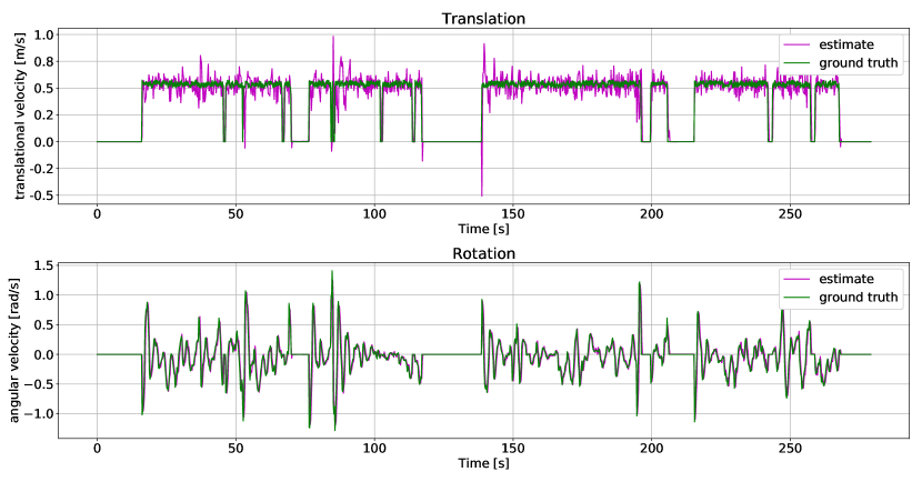
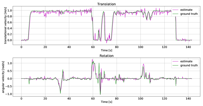
We repeated this experiment on the real robot and the velocity plots in Fig. 4 confirm that our system can effectively recover the robot’s velocities, correctly de-skewing the scan, in real indoor scenarios.

IV-A De-skewing in a SLAM system

Velocities			ATE(m)
$v_{\mathrm{max}}$ (m/s)	$\omega_{\mathrm{max}}$(rad/s)		w/o deskewing	deskewed
0.5	0.5		0.329	$\mathbf{0.113}$
0.5	1.0		0.246	$\mathbf{0.232}$
1.0	1.0		1.018	$\mathbf{0.977}$
1.0	1.5		1.586	$\mathbf{1.520}$
2.0	2.0		11.18	$\mathbf{1.805}$

TABLE II: SLAM comparison

(a)

(b)

(c)

(d)

Figure 5: SLAM Results. (a) Ground truth map (reference). (b) Map constructed using raw scans acquired directly from the LiDAR. (c) Map constructed using processed LiDAR measurements de-skewed by our proposed approach. (d) Estimated trajectories from SLAM, produced by scan matching between consecutive measurements.

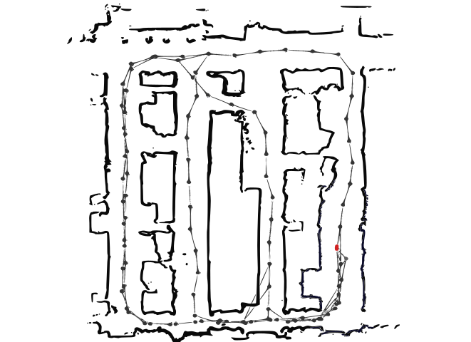
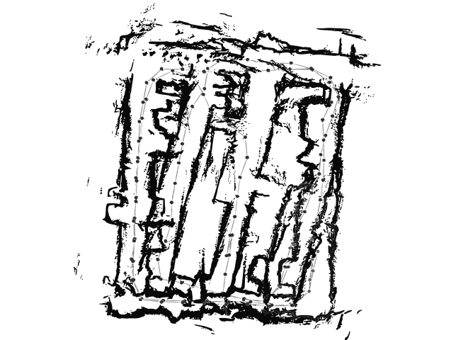
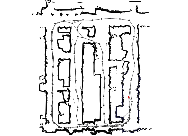
In our final experiment, we used our de-skewing mechanism to pre-process the input of our 2D LiDAR Simultaneous Localization and Mapping (SLAM) system [2]. We run SLAM on three different inputs: the raw (skewed) scans, the ones de-skewed by using the proposed approach, and finally the data de-skewed by using the ground truth. We simulated different exploration runs of the same environment while changing the velocity bounds of the robot. Fig. 5 illustrates the three different maps obtained.

Furthermore, we measure the Absolute Trajectory Error (ATE) between the ground truth trajectory computed by the simulator and the ones estimated by SLAM using the two types of scans. ATE measures the distance between corresponding points of the trajectories, after computing a transformation that makes them as close as possible. For trajectory registration, we used the Horn method [5], while the corresponding poses are associated based on the timestamps. The results are summarized in Tab. II. Consistently, the trajectories obtained by using de-skewed data are substantially closer to the ground truth compared to their skewed counterpart as shown in Fig. 5(d). This is confirmed by the maps generated based on the trajectories and illustrated in Fig. 5. These results are consistent and confirm the importance of the de-skewer since these measurements might induce systematic unrecoverable errors in the registration process.

V Conclusion

In this paper, we presented a simple and effective planar LiDAR de-skewing mechanism based on plane-to-plane registration criteria. To the best of our knowledge, this is the only de-skewing pipeline that does not rely on additional sensors (i.e. IMU, wheel encoders), targeting specifically slow and inexpensive LiDAR s, and enhancing the quality of the scan. For future work, we are planning to integrate the proposed approach in more complex systems, while generalizing the approach for 3D data.

References

- [1] Al-Nuaimi, A., Lopes, W., Zeller, P., Garcea, A., Lopes, C., Steinbach, E.: Analyzing lidar scan skewing and its impact on scan matching. In: 2016 International Conference on Indoor Positioning and Indoor Navigation (IPIN). pp. 1–8. IEEE (2016)
- [2] Colosi, M., Aloise, I., Guadagnino, T., Schlegel, D., Corte, B.D., Arras, K.O., Grisetti, G.: Plug-and-play slam: A unified slam architecture for modularity and ease of use. In: IROS. pp. 5051–5057 (2020). https://doi.org/10.1109/IROS45743.2020.9341611
- [3] Forster, C., Carlone, L., Dellaert, F., Scaramuzza, D.: On-manifold preintegration for real-time visual–inertial odometry. IEEE Transactions on Robotics 33(1), 1–21 (2016)
- [4] He, L., Jin, Z., Gao, Z.: De-skewing lidar scan for refinement of local mapping. Sensors 20(7), 1846 (2020)
- [5] Horn, B., Hilden, H., Negahdaripour, S.: Closed-form solution of absolute orientation using orthonormal matrices. JOSA A 5(7), 1127–1135 (1988)
- [6] Moosmann, F., Stiller, C.: Velodyne slam. In: 2011 ieee intelligent vehicles symposium (iv). pp. 393–398. IEEE (2011)
- [7] Shan, T., Englot, B.: Lego-loam: Lightweight and ground-optimized lidar odometry and mapping on variable terrain. In: IEEE/RSJ International Conference on Intelligent Robots and Systems (IROS). pp. 4758–4765. IEEE (2018)
- [8] Shan, T., Englot, B., Meyers, D., Wang, W., Ratti, C., Rus, D.: Lio-sam: Tightly-coupled lidar inertial odometry via smoothing and mapping. In: 2020 IEEE/RSJ international conference on intelligent robots and systems (IROS). pp. 5135–5142. IEEE (2020)
- [9] Tang, J., Chen, Y., Niu, X., Wang, L., Chen, L., Liu, J., Shi, C., Hyyppä, J.: Lidar scan matching aided inertial navigation system in gnss-denied environments. Sensors 15(7), 16710–16728 (2015)
- [10] Wang, Z., Zhang, L., Shen, Y., Zhou, Y.: D-liom: Tightly-coupled direct lidar-inertial odometry and mapping. IEEE Transactions on Multimedia (2022)
- [11] Xu, W., Zhang, F.: Fast-lio: A fast, robust lidar-inertial odometry package by tightly-coupled iterated kalman filter. IEEE Robotics and Automation Letters 6(2), 3317–3324 (2021)
- [12] Ye, H., Chen, Y., Liu, M.: Tightly coupled 3d lidar inertial odometry and mapping. In: 2019 International Conference on Robotics and Automation (ICRA). pp. 3144–3150. IEEE (2019)
- [13] Zhang, J., Singh, S.: LOAM: lidar odometry and mapping in real-time. In: Fox, D., Kavraki, L.E., Kurniawati, H. (eds.) Robotics: Science and Systems X, University of California, Berkeley, USA, July 12-16, 2014 (2014). https://doi.org/10.15607/RSS.2014.X.007, http://www.roboticsproceedings.org/rss10/p07.html