What is the state of the art? Accounting for multiplicity in machine learning benchmark performance

1 Introduction: Population vs sample state-of-the-art performance

Machine learning methods are commonly evaluated and compared by their performance on data sets from public repositories, where methods can be evaluated under identical conditions and across time. Theoretical results play an important role in machine learning research, but for the last couple of decades the success of increasingly complex methods has pushed the proof towards the pudding: performance on benchmark data sets.

The numbers don’t lie: if method A performs better than method B on a specific data set, that is what it did. But the truth that the numbers tell is limited. We think of a data set, for example a collection of images, as a random sample from an underlying population. In science we are interested in the performance on the population, and the observed performance acts as an estimate. A good estimator gives a reliable result, but overfitting to the data set, originating from wrong use of cross-validation, data leakage and data reuse, can give overly optimistic estimates. An independent test set, often referred to as a hold-out set, is a sample that is not used for development of the method, and gives an unbiased estimator. Competitions and challenges with prize money typically withhold the test set so that it becomes impossible for the participants to use it for development.

Although we know these things we have a tendency to extrapolate the performance metric and interpret it as something about the world rather than something about a data set. If we always appended “on MNIST” when we said so-and-so method had accuracy so-and-so nobody would care. Who cares about MNIST? We hold out data precisely because we want to estimate some sort of long-term behavior on similar data.

An unbiased estimator solves only half of the problem; the variance tells just as much as the bias regarding the quality of a method. For machine learning methods, the sources of variance are plentiful. One is the random nature of the test set, the training set and the validation set. In addition comes the setting of hyperparameters, which can lead to substantial variation, and minor variance sources such as random seeds and stochastic dropouts. The sources of variance that are part of the training are often referred to as influencing the method’s stability or robustness. With knowledge about the behaviour of both the bias and the variance of an estimator, the error can be predicted, often in terms of a confidence interval. It is certainly more useful to know what the lower limit of the 95% confidence interval is, than the observed performance on a specific test set.

The highest ranked performance on a problem is referred to as state-of-the-art (SOTA) performance, and is used, among other things, as a reference point for publication of new methods. As a specific method’s performance on a test set is just an estimate of its true underlying performance, the reported SOTA performances are estimates, and hence come with bias and variance.

State-of-the-art performance increasingly relies on benchmark data sets, often in combination with a challenge or a competition. The practice of hold-out test sets in competitions safe-guards against overoptimistic estimates for the individual classifiers. Data is often released after the competition has ended, and new methods can be compared to the state-of-the-art performance.

As we will show in the subsequent sections, using the highest-ranked performance as an estimate for state-of-the-art is a biased estimator, giving overoptimistic results. The mechanisms at play are those of multiplicity, a topic that is well-studied in the context of multiple comparisons and multiple testing, but has, as far as the authors are aware of, been nearly absent from the discussion regarding state-of-the-art estimates.

Biased state-of-the-art has consequences both for practical implementations and for research itself. A health care provider might want to use some machine learning method for tumour detection, but only if the method correctly classifies at least 80%. The health care provider closely follows updates on state-of-the-art performance, and are ready to invest time and money in a pilot project once the lower bound surpasses 80%. If the state-of-the-art performance is an optimistic estimate, the health care provider has now lost time and money, and perhaps also some faith in research results.

For the research community, the situation is perhaps even more dramatic. The optimistic state-of-the-art estimate is used as a standard for evaluating new methods. Not to say that a new method necessarily needs to beat the current state-of-the-art to catch interest from reviewers and editors, but it certainly helps if its performance is comparable. It has been pointed out (see Section 2) that the incremental increase in performance can obstruct the spread of new ideas that have substantial potential, but just haven’t reached their peak yet.

In this article, we provide a probability distribution for the case of multiple classifiers. We demonstrate the impact of multiplicity through simulated examples. We show how classifier dependency impacts the variance, but also that the impact is limited when the accuracy is high. Finally, we discuss a real-world example; a Kaggle competition from 2020. All code is available at https://github.com/3inar/ninety-nine.

2 Related work

Multiple comparisons is a well-studied subject within statistics, see, e.g., Tukey (1991) for an interesting discussion on some topics of multiple comparisons, among them the confidence intervals. For a direct demonstration of how multiple testing can lead to false discoveries, Bennett et al. (2009) gives an example where brain activity is detected in a (dead) salmon “looking” at photos of people. In the machine learning context, with multiple data sets and classifiers, Demšar (2006) suggests adjusting for multiple testing, according to well-known statistical theory. Our article focuses on the estimate itself and its uncertainty, and not comparison of methods.

The re-use of benchmark datasets has been addressed in several publications. Salzberg (1997) point to the problem that arises because these datasets are static, and therefore run the risk of being exhausted by overfitting. Exhausted public data sets still serve important functions, e.g., a new idea can show to perform satisfactory, even when it is not superior. Thompson et al. (2020) distinguishing between simultaneous and sequential multiple correction procedures. In sequential testing, which is the reality of public datasets, the number of tests is constantly updated. An interesting topic they bring up is the conflict between sharing incentive, open access and stable false positive rate. There are several demonstrations of the vulnerability of re-use of benchmark datasets. Teney et al. (2020) performed a successful attack on the VQA-CP benchmark dataset, that is, they are able to attain high performance with a non-generalisable classifier. They point towards the risk of ML methods capturing idiosyncrasies of a dataset. Torralba and Efros (2011) introduced the game Name That Dataset! motivating their concern of methods being tailored to a dataset rather than a problem. The lack of statistically significant differences among top performing methods is demonstrated by, e.g., Everingham et al. (2015) and Fernández-Delgado et al. (2014).

The same mechanisms of overfitting are present in challenges through multiple submissions to the validation set. Blum and Hardt (2015) introduced an algorithm that releases the public leaderboard score only if there has been significant improvement compared to the previous submission. This will prevent overfitting by hindering adjustments to random fluctuations in the score, and not true improvements of the method. Dwork et al. (2017) use the principles of differential privacy to prevent overfitting to the validation set.

Several publications show that the overfitting is not as bad as expected, and provide possible explanations. Recht et al. (2019) constructed new, independent test sets of CIFAR-10 and ImageNet. They found that the accuracy drop is dramatic, around 10%. However, the order of the best performing methods is preserved, which can be explained by the fact that multiple classes (Feldman et al. (2019)) and model similarity (Mania et al. (2019)) slows down overfitting. Roelofs et al. (2019) compared the results from the private leaderboard (one submission per team) and the public leaderboard (several submissions per team) in Kaggle challenges. Several of their analyses indicate overfitting even though their main conclusion is that there is little evidence of overfitting.

Overfitting and its consequences are avoided in most challenges by withholding the test set so that a method can only be evaluated once and not adapted to the test set performance. Hold-out datasets also prevents wrong use of cross-validation, see, e.g., Fernández-Delgado et al. (2014) and the seminal paper of Dietterich (1998). Another contribution from public challenges is the requirement of reproducibility to collect the prize money, which is a well-known concern in science, see, e.g., Gundersen and Kjensmo (2018). Public challenges typically rank the participants by a (single) performance measure, and can fall victims of Goodhart’s law, paraphrased as “When a measure becomes a target, it ceases to be a good measure.” by Teney et al. (2020). Ma et al. (2021) offers a framework and platform for evaluation of NLP methods, where other aspects such as memory use and robustness are evaluated.

The robustness/stability of a method, and the variability in performance are crucial aspects that the hold-out test set of public challenges does not offer an immediate solution to. Bouthillier et al. (2021) showed empirically that hyperparameter choice and the random nature of the data are two large contributors to variance, whereas data augmentation, dropouts, and weights initialisations are minor contributors. Choice of hyperparameters are often adjusted to validation set results, and the strategies of Blum and Hardt (2015) and Dwork et al. (2017) can hinder that, if implemented by the challenge hosts. Our contribution is a focus on better estimate for state-of-the-art performance under the current conditions, where the approach of Bouthillier et al. (2021) does not apply. Bousquet and Elisseeff (2002) investigate how sampling randomness influences accuracy, both for regression algorithms and classification algorithms, relying on the work of Talagrand (1996) who stated that “A random variable that depends (in a “smooth” way) on the influence of many independent variables (but not too much of any of them) is essentially constant.”

There is a rich literature on various aspects regarding the use of public challenges as standards for scientific publications, see, e.g., Varoquaux and Cheplygina (2022) for a much broader overview than the one given here. Concerns and solutions regarding multiplicity and better performance estimates are active research fields. We contribute to this conversation by shining the light on how multiplicity of classifiers’ performance on hold-out test sets create optimistic estimates of state-of-the-art performance.

3 Multiple classifiers and biased state-of-the-art estimation

3.1 Notation

$$n :\text{number of trials/size of test set}$$

$$\theta :\text{probability of success/probability of correct prediction}$$

$$m :\text{number of experiments/number of classifiers}$$

$$\mathcal{B}ern(\theta) :\text{Bernoulli distribution}$$

$$Y :\text{random variable, indicates if prediction is correct}$$

$$\,\,\,\,Y\sim\mathcal{B}ern(\theta)$$

$$\mathcal{B}(n,\theta) :\text{binomial distribution}$$

$$X :\text{random variable, number of failures in one experiment}$$

$$\,\,\,\,X\sim\mathcal{B}(n,1\text{-}\theta)$$

$$\hat{\theta}(X)=\frac{n-X}{n} :\text{estimator for }\theta,\text{ unbiased}$$

$$P(X=x) :\text{probability of $x$ failures in one experiment}$$

$$P_{x}=P(X\leq x) :\text{probability of at most $x$ failures in one experiment}$$

$$\mathbf{X}=\{X_{1},X_{2},\ldots,X_{m}\} :\text{random sample, number of failures for classifiers }j=1,\ldots,m$$

$$C_{x} :\text{random variable, number of experiments with at most $x$ failures}$$

$$\,\,\,\,C_{x}\sim\mathcal{B}(m,P_{x})$$

$$Z :\text{random variable, the smallest number of failures among all classifiers}$$

$$\theta_{SOTA} :\text{highest probability of correct prediction among all classifiers}$$

$$\hat{\theta}_{SOTA}(\mathbf{X})=\max_{j}\hat{\theta}_{j} :\text{estimator for }\theta_{SOTA},\text{ biased}$$

$$\alpha :\text{significance level}$$

3.2 Two coin-flip examples

Multiplicity is, simply put, how the probability of an outcome changes when an experiment is performed multiple times. Consider $n=20$ flips of a fair coin where the outcome is the number of heads, referred to as the number of successes in a binomial distribution, $\mathcal{B}(n,\theta)$, where the probability of success is $\theta=0.5$. Let the random variable $X$ denote the number of failures, $X\sim\mathcal{B}(n,1\text{-}\theta)$. The probability of $15$ heads or more corresponds to observing $x=n-15$ tails or less, that is, the cumulative distribution $P(X\leq x|n,1\text{-}\theta)$. This corresponds to the cumulative distribution for the estimator $\hat{\theta}(X)=\frac{n\text{-}X}{n}$, and we have that $P(\hat{\theta}(X)\geq\frac{n\text{-}x}{n})=P(X\leq x)=0.02069$ for $\hat{\theta}\geq 0.75$. In other words, if $\theta=0.5$, there is a probability of $0.02069$ that the estimate is $0.75$ or above in a series of $n=20$ trials. The probability of exactly $x=5$ can be calculated from the probability mass function (pmf) $P(X=x|n,1\text{-}\theta)=0.01479$, but the interest usually lies with the cumulative distribution. We focus on the case where $X\leq x$, but it is straightforward to substitute $P(X\leq x)$ for $P(X=x)$ in the following.

If we fix $x$ we can define the experiment described above as a Bernoulli trial, where success is defined as $X\leq x$, with corresponding probability $P(X\leq x)$, which we from now on write as $P_{x}$ for ease of notation. If we perform the coin-flip experiment $m$ times, and success is defined as $X\leq x$, we have a series of $m$ Bernoulli trials, and the number of successes follow the binomial distribution $\mathcal{B}(m,P_{x})$. Let $C_{x}$ be the random variable that denotes the number of successful experiments. The probability of, for example, $C_{x}=10$ experiments with at most $x=5$ tails, is calculated from the pmf $P(C_{x}=10|m,P_{x})$. Of special interest is the case where at least one experiment succeeds, $P(C_{x}>0)=1-P(C_{x}=0)$. In our example, if the coin-flip experiment is performed $m=100$ times, the probability of observing $15$ heads or more at least once is $P(C_{x}>0|m,P_{x})=1-P(C_{x}=0|m,P_{x})$, with $P_{x}=0.02069$ from above. In the estimation context, we have that although the probability of $\hat{\theta}\geq 0.75$ is only $0.02069$ for the individual experiments, the probability of at least one $\hat{\theta}\geq 0.75$ is $0.8765$ when the experiment is performed $m=100$ times.

Consider an experiment where a coin is flipped $n=20$ times, and the number of successes is the number of times a classifier correctly predicts the outcome. An unbiased estimator for a classifier’s probability of correct prediction, $\theta$, is ${\hat{\theta}=(n-X)/n}$, where $X$ is the number of failures. The corresponding estimate is referred to as accuracy. The true state-of-the-art for coin-flip classifiers is $\theta_{SOTA}=0.5$, since it is impossible to train a classifier to predict coin flips. If $m=1,000$ classifiers independently give their predictions for $n=20$ flips, we can consider this as a binomial experiment with $1,000$ Bernoulli trials, where the probability of success is the individual classifier’s probability of $n-X\leq n-x$ correct predictions. The probability of at least one classifier achieving an accuracy of at least $0.90$ is $1-P(C_{x}=0|m,P_{x})=0.1823$, where $P_{x}=P(X\leq 18|n,1\text{-}\theta)=0.00020$. This means that using the top-ranked method as an estimate and ignoring multiplicity there is a substantial risk of overestimating the state-of-the-art.

3.3 The probability distribution of $\hat{\theta}_{SOTA}$

We define the SOTA probability of correct prediction, $\theta_{SOTA}$, as the highest probability of correct prediction among all classifiers applied to a test set, in accordance with the common set-up for public competition. Of interest is $P(\hat{\theta}_{SOTA}|m,n,\theta)$, the probability of $\hat{\theta}_{SOTA}$, being the estimated state of the art from taking the highest ranked classifier, given the number of classifiers, the size of the test set, and the probabilities of correct prediction, $\theta=\{\theta_{1},\ldots,\theta_{m}\}$.

We will in the following assume independent classifiers, and discuss dependency in Section 4. We demonstrate the impact of multiplicity in the simple case of identical probabilities of correct prediction, $\theta_{j}=\theta$ for all classifiers, $j=1,\ldots,m$, and where $\theta_{SOTA}=\theta$. We discuss non-identical classifiers in Section 4.2.

Let $n$ denote the size of the test set, $m$ be the number of classifiers, and $\theta$ be the probability of correct prediction. Let $X$ be the random variable that denotes the number of failures (wrong predictions) for a given classifier. We have that $X\sim\mathcal{B}(n,1\text{-}\theta)$. We denote by $P_{x}$ the cumulative distribution $P(X\leq x)$. The random sample, $\mathbf{X}=\{X_{1},X_{2},\ldots,X_{m}\}$ consists of the number of wrong predictions for each classifier $j=1,\ldots,m$ on a test set. Let $C_{x}$ be the random variable that denotes the number of classifiers with at most $x$ failures. We have that $C_{x}\sim\mathcal{B}(m,P_{x})$, because each classifier will independently have a probability $P_{x}$ of having at most $x$ wrong predictions.

We are interested in the probability of at least one classifier having at most $x$ wrong predictions, because it corresponds to the probability function of the $\hat{\theta}_{SOTA}$ estimator, $P(\hat{\theta}_{SOTA}>\frac{n-x}{n})$, in other words, at least one $\hat{\theta}_{j}>\frac{n-x}{n}$. We can derive this from $C_{x}$:

$$P(C_{x}>0|m,n,\theta).$$ (1)

Note that this corresponds to the cumulative distribution function (cdf) $F(z)$ for the random variable $Z$, denoting the most wrong predictions among all classifier. We have cdf $F(z)$, the probability that the most wrong predictions among all classifiers is less than or equal to a number $z$, can easily be derived from the binomial distribution

$$F(z) =P(C_{z}>0|m,n,\theta)=1-P(C_{z}=0|m,P_{z})$$

$$=1-(1-P_{z})^{m}.$$ (2)

Let $f(z)$ denote the probability mass function of $Z$. We then have

$$f(z) =F(z)-F(z-1)=1-(1-P_{z})^{m}-\{1-(1-P_{z-1})^{m}\}$$

$$=(1-P_{z-1})^{m}-(1-P_{z})^{m}=$$

$$=(1-\sum_{\ell=0}^{z-1}P(Z=\ell))^{m}-(1-\sum_{\ell=0}^{z-1}P(Z=\ell)-P(Z=z))^{m}$$

$$=-\sum_{k=1}^{m}(-1)^{k}\binom{m}{k}(1-\sum_{\ell=0}^{z-1}P(Z=\ell))^{m-k}P(Z=z)^{k}.$$ (3)

The last line is derived by binomial expansion. The practical relevance of the binomial expansion is limited by the need to approximate binomial coefficient for large $m$. From Eq. 3.3, the expected value and variance can easily be calculated. An example of $F(z)$ can be seen in Fig. 2, and the corresponding $f(z)$ in Fig. 3. The pmf $f(z)=P(Z=z)$ denotes the probability of at least one classifier having exactly $z$ wrong predictions, and no classifiers having fewer than $z$ wrong predictions.

3.4 A simulated public competition example

The multiplicity mechanisms described above apply to public competitions where several teams submit their predictions on a test set. Winning teams are those with highest accuracy, $\max_{j}\hat{\theta}_{j}$, where $\hat{\theta}_{j}=(n-x_{j})/n$ is the accuracy of a classifier $j$ on the test set. This is often referred to as the state of the art, and hence, we have that $\hat{\theta}_{SOTA}(\mathbf{x})=\max_{j}\hat{\theta}_{j}$. As exemplified in Section 3.2, multiplicity biases the estimation of $\theta_{SOTA}$, and Section 3.3 gives us the tools to analyze its impact. In the following, we will use a significance level of $\alpha=0.05$ and two-sided confidence intervals.

Consider a classification problem with a test set of size $n=3,000$, and a classifier with probability of correct prediction $\theta=0.90$. The pmf of a single classifier is shown as a histogram in Fig. 1. The 95% confidence interval for $\theta$ if we have observed $\hat{\theta}=0.90$ is $(0.8887,0.9105)$, and we denote it by $(\theta_{\alpha/2},\theta_{1\text{-}\alpha/2})$.

If there are $m=1,000$ classifiers, each with probability of correct prediction $\theta=0.90$, the probability of at least one team achieving at least $\theta_{1\text{-}\alpha/2}$ is close to 1. This comes as no surprise given the definition of a confidence interval. It means that we can be almost certain that the accuracy of the top ranked classifier, which is the default SOTA, is above the upper limit of the confidence interval of the true performance.

On the other hand, it is straightforward to show that if each individual classifier has a probability of $P_{x}=0.00002532$ for at most $x$ failures, then, with a probability of $\alpha/2$, at least one team will achieve at least $\hat{\theta}=0.9213$. We denote this by $\theta^{m}_{1\text{-}\alpha/2}$, the multiplicity-adjusted upper limit of the $(1\text{-}\alpha)$ confidence interval.

Similarly, the expected value of $\hat{\theta}_{SOTA}$ can easily be calculated from Eq. 3.3, and we have $E(\hat{\theta}_{SOTA})=0.9173$. Both are optimistic estimates, knowing that $\theta_{SOTA}$ is $0.90$.

Within the competition context, this is not necessarily a problem, because each team has the same probability of achieving the highest accuracy given that they have the same $\theta$. In a scientific context, using $\max_{j}\hat{\theta}_{j}$ as an estimate for $\theta_{SOTA}$ without multiplicity corrections is problematic. Consider a new classifier with probability of correct prediction $\theta_{m+1}=\theta_{1\text{-}\alpha/2}$ from above, displayed as the red curve in Fig. 1. By common scientific standards, the expected performance, $E(\hat{\theta}_{m+1})=\theta_{m+1}$ is considered significantly better than the expected performance of any of the $1,000$ classifiers with $\theta=0.90$, and is of interest to the research community. But the probability of this classifier beating the upper limit of the multiplicity adjusted confidence interval is very low: $P(\hat{\theta}_{m+1}\geq\theta^{m}_{1\text{-}\alpha/2})=0.0190$, and can be seen as the red area in Fig. 1. Similarly, $P(\hat{\theta}_{m+1}\geq E(\hat{\theta}_{SOTA}))=0.0996$, seen as the blue plus red area in Fig. 1. This means that by using the maximum accuracy as SOTA, we can expect that 9 out of 10 classifiers that are in fact better will still be naively considered worse.

The probability mass functions of single $\hat{\theta}$.

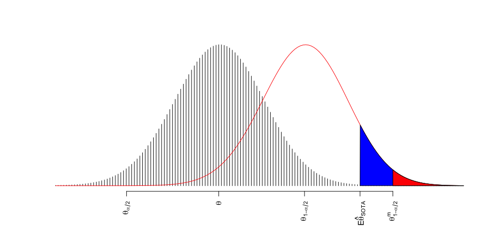
Figure 1: The grey histogram shows the pmf of a classifier with probability of correct prediction $\theta$. The red curve is the pmf of a classifier with probability of correct prediction $\theta_{1\text{-}\alpha/2}$, the upper limit of the $95\%$ CI for $\hat{\theta}(\mathbf{x})=\theta$. $E(\hat{\theta}_{SOTA})$ denotes the expected value of the highest ranked among $m=1,000$ classifiers. $\theta^{m}_{1\text{-}\alpha/2}$ is the multiplicity corrected upper limit of the $95\%$ CI. The shaded areas corresponds to $P(\hat{\theta}_{m+1}\geq\theta^{m}_{1\text{-}\alpha/2})$ (red) and $P\big{(}\hat{\theta}_{m+1}\geq E(\hat{\theta}_{SOTA})\big{)}$ (blue+red).

The cumulative distribution function, $F(z)$ from Eq. 3.3, is displayed in Fig. 2, and describes the cumulative probability of at least one classifier having at most $z$ failures. Or, in other words, the cumulative probability of maximum accuracy. The number of failures are displayed on the top horizontal axis, and the corresponding accuracy on the bottom horizontal axis. Note that the horizontal axis is reversed compared to Fig. 1.

Cumulative distribution function, $F(z|m,n,\theta)$, for at least one classifier having at most $z$ failures.

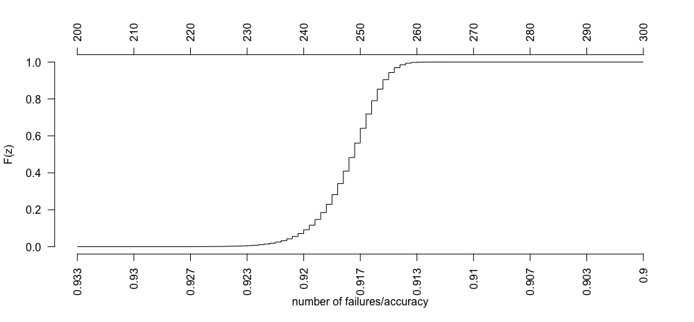
Figure 2: The figure shows the cumulative distribution function for at least one classifier having at most $z$ failures. The horizontal axis denotes the number of failures, $z$, on top and the accuracy at the bottom.

The corresponding pmf, $f(z)$ from Eq. 3.3, is displayed as a histogram in Fig. 3.

Probability mass function, $f(z|m,n,\theta)$, for the smallest number of failures, $z$, among all classifiers.

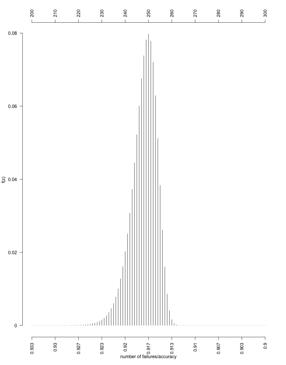
Figure 3: The figure shows the corresponding pmf for Fig. 2. The horizontal axis denotes the number of failures, $z$, on top and the corresponding accuracy at the bottom.

From Eq. 3.3 we get the expected value and variance. For $m=1,000$, $n=3,000$ and $\theta=0.9$ this corresponds to $E(\hat{\theta}_{SOTA})=0.9173$ with a standard deviation of $0.001817$. We can see how different values for $m$, $n$ and $\theta$ affects the $\hat{\theta}_{SOTA}$ distribution in Table 1.

Expected values and standard deviations for $\hat{\theta}_{SOTA}$

m	n	$\theta$	expected value	standard deviation
1,000	3,000	0.85	0.8707	0.002197
1,000	3,000	0.90	0.9173	0.001817
1,000	3,000	0.95	0.9624	0.001277
100	3,000	0.90	0.9135	0.002250
500	3,000	0.90	0.9163	0.001923
1,000	1,000	0.90	0.9294	0.003007
1,000	10,000	0.90	0.9096	0.001022

Table 1: The expectation and standard deviation for the SOTA estimator with varying test set size, number of classifiers and probability of correct prediction. The bold line is the example used in Fig. 3.

4 Non-i.i.d.

The probability distribution in Section 3.4 is based on independent classifiers with identical $\theta$s. This assumption is rarely true in practice. A classifier’s ability to perform better than random guesses is due to correlation between features and labels in a training set. The teams will pick up on many of the same features and correlations, regardless of which method they choose. In addition, many teams will use different versions of related methods. We investigate dependency and non-identical classifiers, and the impact on the bias. Table 2 gives an overview, details are in the following sections.

Upper bounds, expected values and standard deviations for $\hat{\theta}_{SOTA}$

section	independent	identical	upper 95% CI	expected value	standard deviation
3.4	YES	YES	0.9213	0.9173	0.001817
4.1	NO	YES	0.9207	0.9140	0.003481
4.1	NO∗	YES	0.9173	0.9140	0.001484
4.2	YES	NO	0.9177	0.9130	0.002129
4.3	NO	NO	0.9173	0.9101	0.003649

Table 2: The upper bound of the 95% CI, the expectation and standard deviation for the SOTA estimator for different combinations of independency and identicality.

4.1 Dependent, identical classifiers

The dependency between two classifiers $j,k$ can be described by their correlation, $\rho_{jk}$. Let $Y_{j}$ be the Bernoulli variable with value $1$ if classifier $j$ predicts a data point correctly. We have $P(Y_{j}=1)=\theta_{j}$, and $\theta_{j}=\theta$ for classifiers with equal probability of success. Mania et al. (2019) calculated the similarity, defined as the fraction of two models giving the same output, which is equivalent to

$$P\big{(}\{Y_{j},Y_{k}\}=\{0,0\}\big{)}+P(\{Y_{j},Y_{k}\}=\{1,1\})$$ (4)

$$=(1-\theta_{j})(1-\theta_{k})+\theta_{j}\theta_{k}$$

for independent models. For dependent models with correlation $\rho_{jk}$, this becomes

$$(1-\theta_{j})(1-\theta_{k})+\theta_{j}\theta_{k}+2\rho_{jk}\sqrt{\theta_{j}\theta_{k}(1-\theta_{j})(1-\theta_{k})}.$$ (5)

By setting $\theta_{j}=\theta$ and $\rho_{jk}=\rho$, $\rho$ can easily be estimated from the estimations of $\theta$, $P\big{(}\{Y_{j},Y_{k}\}=\{0,0\}\big{)}$ and $P(\{Y_{j},Y_{k}\}=\{1,1\})$. In Mania et al. (2019), they used the average accuracy for top-performing ImageNet models, $\hat{\theta}=0.756$. For details, see Mania et al. (2019). Note that these are multi-class problems, so a lower accuracy than for binary classification problems is to be expected. From their calculated similarity of $0.85$, the estimated correlation is $0.36$.

Boland et al. (1989) describes dependency in the majority systems context, with $\rho_{0j}=\text{corr}(Y_{0},Y_{j}),\,j=1,\ldots m$, and the $Y_{j}$s are independent given $Y_{0}$. This gives $\rho_{jk}=\rho_{0j}^{2}$. The observations from $Y_{0}$ does not contribute directly to $\hat{\theta}_{SOTA}$, but can be seen as, e.g., the influence that a common training set has on the classifiers. For $\rho_{0j}=1$, we have $m$ identical classifiers, and an unbiased E($\hat{\theta}_{SOTA})=\theta$. For $\rho_{0j}=0$, we have $m$ independent classifiers, and the situation is identical to the one described in Section 3.3.

The binomial distribution for dependent Bernoulli trials is not an easy problem, see, e.g., Ladd (1975) and Hisakado et al. (2006). We here demonstrate by simulation how dependency reduces the bias. We use the estimated correlation from Mania et al. (2019), which corresponds to $\rho_{0j}=0.6$ in the multiplicity set-up with an external $Y_{0}$.

We use the set-up from Section 3.4 with $m=1,000$ classifiers, test set size $n=3,000$, and probability of correct prediction $\theta=0.90$. We simulate two scenarios; one where $Y_{0}$ is random, and one where the $y_{0}$’s are fixed with exactly $(n-x)/n=0.90$ correct predictions. The fixed scenario can correspond to fixed training conditions, e.g., models pre-trained on ImageNet. The random scenario picks up the randomness in, e.g., a training set. Although all teams have the same training set, the training set is a random sample.

The upper bound of the $95\%$ confidence interval for the dependent classifiers is at $0.9173$ for the fixed $y_{0}$ and $0.9207$ for the random $Y_{0}$, but they have the same expected value.

Minimum number of failures in $m=1,000$ classifiers.

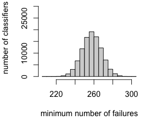
(a) $\rho_{0j}=0.6$, random $Y$

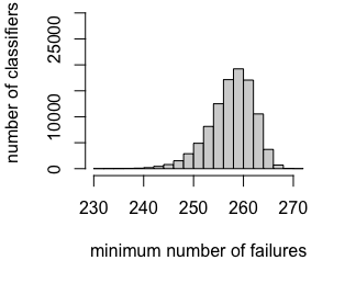
(b) $\rho_{0j}=0.6$, fixed $y$

Figure 4: The minimum number of failures in $100,000$ simulations, with probability of success $\theta=0.9$.

Note that, with $\theta=0.90$, the similarity as described by Mania et al. (2019) is $0.82$ for two independent classifiers. When the probability of correct prediction is high, there is little room for variation between classifiers, and the inherent similarity is high.

4.2 Non-identical, independent classifiers

The Poisson Binomial distribution, see, e.g., Wang1993, describes the sum of $n$ non-identical independent Bernoulli trials with success probabilities $p_{1},p_{2},\ldots,p_{n}$. The pmf for $K$ number of successes is

$$P(K=k)=\sum\limits_{{A\in G_{k}}}\prod\limits_{{i\in A}}p_{i}\prod\limits_{{j\in A^{c}}}(1-p_{j}),$$ (6)

where $G_{k}$ is all subsets that can be selected from {1, 2, …, n}.

In the multiple classifier context, we are interested in generalising Eq. 3.3 to the non-identical case.

$$F(z)=P(C_{z}>0|m,n,\mathbf{\theta})=1-P(C_{z}=0|m,n,\mathbf{\theta}),$$ (7)

where $P(C_{z}=0)$ corresponds to $0$ classifiers with non-identical probabilities of success, $P(Z\leq z|\theta_{j})$. The cdf is

$$F(z) =1-\sum\limits_{{A\in G_{0}}}\prod\limits_{{i\in A}}P(Z\leq z|\theta_{i})\prod\limits_{{j\in A^{c}}}(1-P(Z\leq z|\theta_{j}))$$

$$=1-\prod\limits_{j=1}^{m}\big{(}1-P(Z\leq z|\theta_{j})\big{)}.$$ (8)

The pmf is

$$f(z) =F(z)-F(z-1)$$

$$=1-\prod\limits_{j=1}^{m}\big{(}1-P(Z\leq z|\theta_{j})\big{)}-\{1-\prod\limits_{j=1}^{m}\big{(}1-P(Z\leq z\text{-}1|\theta_{j})\big{)}\}$$

$$=\prod\limits_{j=1}^{m}\big{(}1-P(Z\leq z\text{-}1|\theta_{j})\big{)}-\prod\limits_{j=1}^{m}\big{(}1-P(Z\leq z|\theta_{j})\big{)}$$ (9)

$$=\prod\limits_{j=1}^{m}\big{(}1-\sum\limits_{k=0}^{z\text{-1}}\binom{n}{k}(1-\theta_{j})^{k}\theta_{j}^{n\text{-}k}\big{)}-\prod\limits_{j=1}^{m}\big{(}1-\sum\limits_{k=0}^{z}\binom{n}{k}(1-\theta_{j})^{k}\theta_{j}^{n\text{-}k}\big{)}$$

Analytically, it is more complex than the case of identical classifiers, but it is easy to simulate.

We use a similar set-up as in Section 3.4 with $m=1,000$ classifiers, test set size $n=3,000$, and probabilities of correct prediction $\theta=\{\theta_{1},\ldots,\theta_{m}\}$, where $\min\theta=0.875,\,\max\theta=0.90$, and they are equally spaced.

The simulated non-identical upper bound of the 95% confidence interval is $0.9177$, with $100,000$ repetitions. The $E(\hat{\theta}_{SOTA})$ is $0.9129$, with standard deviation of $0.0021$. The cdf and pmf are displayed in Fig. 5 and Fig. 6.

Cumulative distribution function for non-identical classifiers.

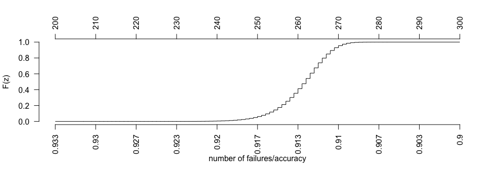
Figure 5:

Probability mass function for non-identical classifiers.

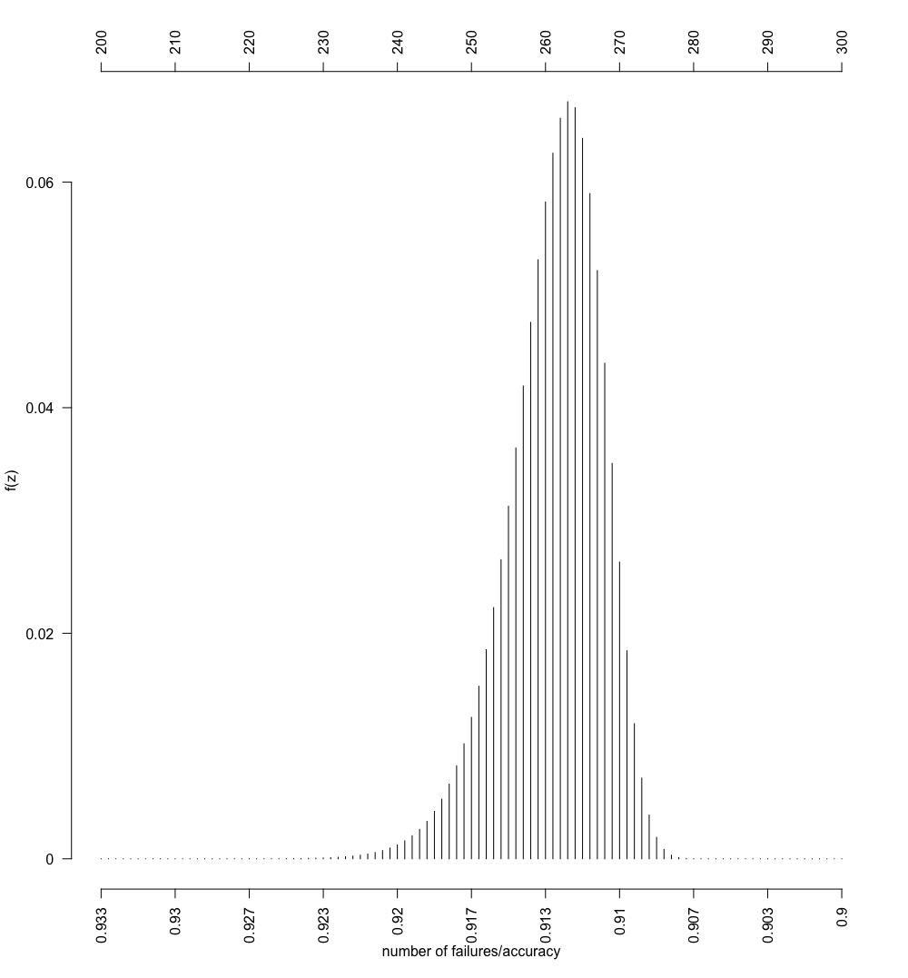
Figure 6:

4.3 Non-identical, dependent classifiers

The most complex, but also the most realistic case, is where classifiers are non-identical and dependent. An analytical solution is not known Hisakado et al. (2006), but simulations are easy. The results of Boland et al. (1989) are easily extended, and we have that

$$P(Y_{j}|Y_{0}=1) =\frac{\rho\sqrt{\theta_{j}(1-\theta_{j})\theta_{0}(1-\theta_{0})}+\theta_{j}\theta_{0}}{\theta_{0}}$$

$$P(Y_{j}|Y_{0}=0) =\frac{-\rho\sqrt{\theta_{j}(1-\theta_{j})\theta_{0}(1-\theta_{0})}+\theta_{j}(1-\theta_{0})}{(1-\theta_{0})}$$ (10)

We get the a the simulated dependent upper bound of the 0.95 confidence interval of $0.91733$, with $100,000$ repetitions.

5 Discussion

We have addressed the mechanisms of multiplicity and how they affect the bias of the SOTA estimator. When accuracy is used as a performance measure, the exact probability distribution can be provided, and known analyses methods can be engaged. The bias in SOTA is substantial in our example, and possibly hinders new methods to attract interest from the scientific community. We have also demonstrated that dependency might not have a big impact on the bias when the probability of correct prediction is already high. The exception is when the dependency is very strong.

The work presented here focuses on the simple case with an analytical solution, and where the probabilities of correct prediction are known. In the public competition or public data set context there are many factors that come in to play, making the bias calculations everything but straightforward. We discuss here an example, the SIIM-ISIC Melanoma Classification competition from 2020 because it follows many of the common structures of public challenges. The winning team chose many of the verified strategies from Section 2.

The SIIM-ISIC Melanoma Classification competition consisted of more than $40,000$ images of skin lesions, split into training ($33,126$), validation ($3,295$) and test set ($7,687$) from various sites. The data set is highly imbalanced, with less than $2\%$ melanomas in the training set, which reflects the reality in many cancer detection situations. A full description can be found in Rotemberg et al. (2021). The size of the test set is smaller than the recommendations of, e.g., Roelofs et al. (2019), but reflects the reality of benchmark datasets and public challenges, as seen, e.g., in the overview of Willemink et al. (2020). We want to emphasise that the shortcomings of this competition are not unique, and that is precisely why it serves as a useful example. Participants were allowed to use additional data for training if the data was shared on the competition web site. The prize money was set to $10,000$ USD for the best-performing method, measured as AUC on the hold-out test set, published in the private leaderboard. Participants could get intermediate results from the validation set, published on a public leaderboard.

The team ‘All Data Are Ext’ consisting of three Kaggle Grandmasters won the competition, achieving an AUC of $0.9490$ on the test set, and their method and strategy is explained in Ha et al. (2020). Although we show that the AUC is an optimistic estimate for the melanoma detection state-of-the-art, we do not question their rank in the challenge. Quite the contrary; the research in Section 2 supports their strategies. Their AUC decreased from the public to the private leaderboard, but it was still within the confidence interval, suggesting that they have avoided overfitting. They had a low rank on the public leaderboard (880th out of 3300), and they have avoided the general overfitting that can be seen in Fig. 7.

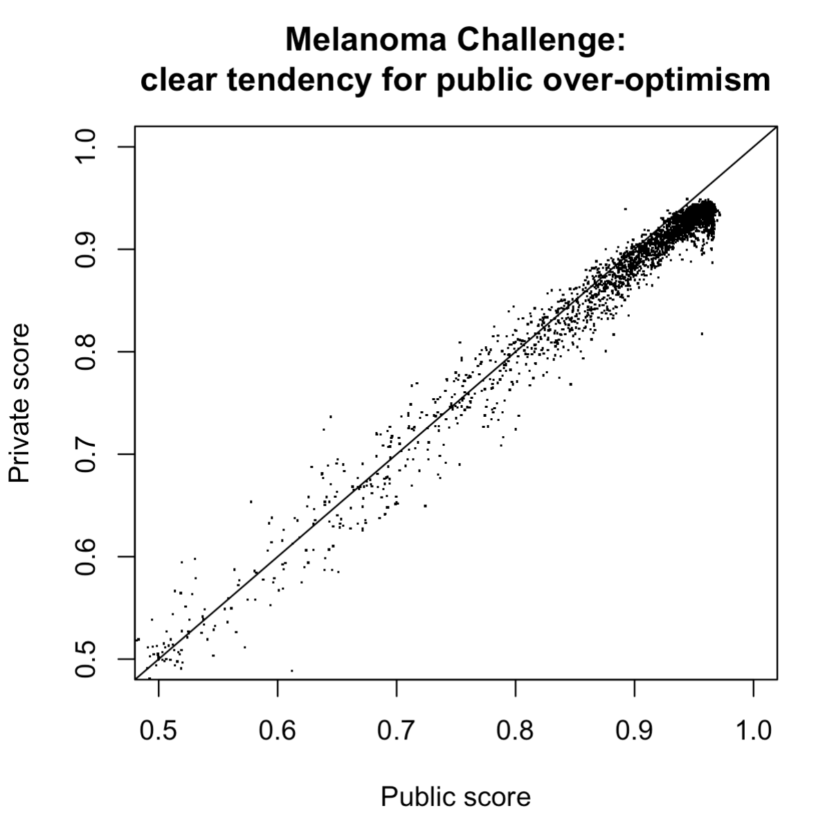
Figure 7: The line indicates public=private scores. There is a strong general tendency of overfitting.

To avoid overfitting, they used additional data from previous years’ competitions, and they also did data augmentation. They chose ensemble learning as a strategy to avoid overfitting, a strategy implicitly supported by Talagrand (1996). They also trained on multiple classes, a strategy that Feldman et al. (2019) showed will slow down the overfitting.

To estimate multiplicity effect on the AUC scores is not as straightforward as with accuracy. The uncertainty of AUC can be calculated through bootstrapping, but without access to the predictions for each data point in the test set, the analyst must make some assumptions about the shape of the ROC curve. Fig. 8 shows different shapes of ROC curves and their confidence intervals. Fig. 9 shows corresponding plots for classifier predictions.

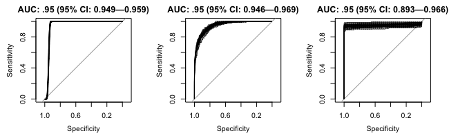
Figure 8: ROC curves with an AUC of .95 can look different. Above are three ROC curves ordered from low variance AUC to high variance

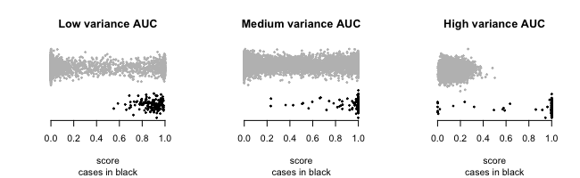
Figure 9: Scores behind each of the above curves. The variability in the AUC curves has to do with thhe way in which the distributions of scores for the two classes overlap. A high-variance curve has mostly low overlap in scores but high variance for the cases, meaning that a small handful of observations decide the shape of the curve. (Recall that an ROC curve is built “backward:” the threshold moves from left to right along the scores and the corresponding operating characteristics are place in the plot from right to left)

However, with high AUC, the shape has less impact, and the analyst’s choices are not suggestive of the overall conclusion. If we assume i.i.d. classifiers and AUC = $0.9352$, the the upper bound of the $95\%$ confidence interval is $0.9490$, same as the winning team. And since there are $427$ teams with AUC $>0.9352$, we can expect observations outside the confidence interval. The conclusion should be that although ‘All Data Are Ext’ did win the competition according to the criteria, the AUC should not be used as the new SOTA. This analysis show that with simple means a more sober SOTA estimate can be communicated. A more elaborate analysis can be done through simulation set-ups, and will decrease the SOTA even further. But the main conclusion remains the same; highest-ranked performance is not the state-of-the-art, but rather an optimistic estimate.

This work shows that a multiplicity-adjusted state-of-the-art estimate can be calculated fairly easily through bootstrapping, and can serve as a better reference point when introducing new methods to the scientific community.

References

- Tukey [1991] John W Tukey. The philosophy of multiple comparisons. Statistical Science, 6:100–116, 1991. URL https://www.jstor.org/stable/2245714#metadata_info_tab_contents.
- Bennett et al. [2009] Craig M Bennett, Abigail A Baird, Michael B Miller, and George L Wolford. Neural correlates of interspecies perspective taking in the post-mortem atlantic salmon: An argument for multiple comparisons correction. Neuroimage, 47:S125, 2009.
- Demšar [2006] Janez Demšar. Statistical comparisons of classifiers over multiple data sets. Journal of Machine Learning Research, 7:1–30, 2006.
- Salzberg [1997] Steven L. Salzberg. On comparing classifiers: Pitfalls to avoid and a recommended approach. Data Mining and Knowledge Discovery, 1:317–328, 1997. ISSN 13845810. doi: 10.1023/A:1009752403260/METRICS. URL https://link.springer.com/article/10.1023/A:1009752403260.
- Thompson et al. [2020] William Hedley Thompson, Jessey Wright, Patrick G. Bissett, and Russell A. Poldrack. Dataset decay and the problem of sequential analyses on open datasets. eLife, 9:1–17, 5 2020. ISSN 2050084X. doi: 10.7554/ELIFE.53498.
- Teney et al. [2020] Damien Teney, Ehsan Abbasnejad, Kushal Kafle, Robik Shrestha, Christopher Kanan, and Anton van den Hengel. On the value of out-of-distribution testing: An example of goodhart’s law. Advances in Neural Information Processing Systems, 33:407–417, 2020.
- Torralba and Efros [2011] Antonio Torralba and Alexei A. Efros. Unbiased look at dataset bias. Proceedings of the IEEE Computer Society Conference on Computer Vision and Pattern Recognition, pages 1521–1528, 2011. ISSN 10636919. doi: 10.1109/CVPR.2011.5995347.
- Everingham et al. [2015] Mark Everingham, S. M.Ali Eslami, Luc Van Gool, Christopher K.I. Williams, John Winn, and Andrew Zisserman. The pascal visual object classes challenge: A retrospective. International Journal of Computer Vision, 111:98–136, 1 2015. ISSN 15731405. doi: 10.1007/S11263-014-0733-5/FIGURES/27. URL https://link.springer.com/article/10.1007/s11263-014-0733-5.
- Fernández-Delgado et al. [2014] Manuel Fernández-Delgado, Eva Cernadas, Senén Barro, Dinani Amorim, and Amorim Fernández-Delgado. Do we need hundreds of classifiers to solve real world classification problems? Journal of Machine Learning Research, 15:3133–3181, 2014. URL http://www.mathworks.es/products/neural-network.
- Blum and Hardt [2015] Avrim Blum and Moritz Hardt. The ladder: A reliable leaderboard for machine learning competitions. pages 1006–1014. PMLR, 6 2015. URL https://proceedings.mlr.press/v37/blum15.html.
- Dwork et al. [2017] Cynthia Dwork, Vitaly Feldman, Moritz Hardt, Toniann Pitassi, Omer Reingold, and Aaron Roth. Guilt-free data reuse. Communications of the ACM, 60:86–93, 4 2017. ISSN 15577317. doi: 10.1145/3051088.
- Recht et al. [2019] Benjamin Recht, Rebecca Roelofs, Ludwig Schmidt, and Vaishaal Shankar. Do imagenet classifiers generalize to imagenet? pages 5389–5400. PMLR, 5 2019. URL https://proceedings.mlr.press/v97/recht19a.html.
- Feldman et al. [2019] Vitaly Feldman, Roy Frostig, and Moritz Hardt. The advantages of multiple classes for reducing overfitting from test set reuse. pages 1892–1900. PMLR, 5 2019. URL https://proceedings.mlr.press/v97/feldman19a.html.
- Mania et al. [2019] Horia Mania, John Miller, Ludwig Schmidt, Moritz Hardt, and Benjamin Recht. Model similarity mitigates test set overuse. Advances in Neural Information Processing Systems, 32, 2019.
- Roelofs et al. [2019] Rebecca Roelofs, Vaishaal Shankar, Benjamin Recht, Sara Fridovich-Keil, Moritz Hardt, John Miller, and Ludwig Schmidt. A meta-analysis of overfitting in machine learning. Advances in Neural Information Processing Systems, 32, 2019. URL https://www.kaggle.com/kaggle/meta-kaggle.
- Dietterich [1998] Thomas G. Dietterich. Approximate statistical tests for comparing supervised classification learning algorithms. Neural Computation, 10:1895–1923, 10 1998. ISSN 0899-7667. doi: 10.1162/089976698300017197. URL https://direct.mit.edu/neco/article/10/7/1895/6224/Approximate-Statistical-Tests-for-Comparing.
- Gundersen and Kjensmo [2018] Odd Erik Gundersen and Sigbjørn Kjensmo. State of the art: Reproducibility in artificial intelligence. Proceedings of the AAAI Conference on Artificial Intelligence, 32:1644–1651, 4 2018. ISSN 2374-3468. doi: 10.1609/AAAI.V32I1.11503. URL https://ojs.aaai.org/index.php/AAAI/article/view/11503.
- Ma et al. [2021] Zhiyi Ma, Kawin, Ethayarajh, Tristan Thrush, Somya Jain, Ledell Wu, Robin Jia, Christopher Potts, Adina Williams, and Douwe Kiela. Dynaboard: An evaluation-as-a-service platform for holistic next-generation benchmarking. Advances in Neural Information Processing Systems, 34:10351–10367, 12 2021. URL https://eval.ai.
- Bouthillier et al. [2021] Xavier Bouthillier, Pierre Delaunay, Mirko Bronzi, Assya Trofimov, Brennan Nichyporuk, Justin Szeto, Nazanin Mohammadi Sepahvand, Edward Raff, Kanika Madan, Vikram Voleti, Samira Ebrahimi Kahou, Vincent Michalski, Tal Arbel, Chris Pal, Gael Varoquaux, and Pascal Vincent. Accounting for variance in machine learning benchmarks. Proceedings of Machine Learning and Systems, 3:747–769, 3 2021.
- Bousquet and Elisseeff [2002] Olivier Bousquet and André Elisseeff. Stability and generalization. Journal of Machine Learning Research, 2:499–526, 2002. URL http://sensitivity-analysis.jrc.cec.eu.int/.
- Talagrand [1996] Michel Talagrand. A new look at independence. The Annals of Probability, 24:1–34, 1996. URL https://www.jstor.org/stable/2244830#metadata_info_tab_contents.
- Varoquaux and Cheplygina [2022] Gaël Varoquaux and Veronika Cheplygina. Machine learning for medical imaging: methodological failures and recommendations for the future. npj Digital Medicine 2022 5:1, 5:1–8, 4 2022. ISSN 2398-6352. doi: 10.1038/s41746-022-00592-y. URL https://www.nature.com/articles/s41746-022-00592-y.
- Boland et al. [1989] Philip J. Boland, Frank Proschan, and Y. L. Tong. Modelling dependence in simple and indirect majority systems. Journal of Applied Probability, 26:81–88, 3 1989. ISSN 0021-9002. doi: 10.2307/3214318. URL https://www.cambridge.org/core/journals/journal-of-applied-probability/article/abs/modelling-dependence-in-simple-and-indirect-majority-systems/070D6335BDDDDC7AF4D70BC9B21B0B7B.
- Ladd [1975] Daniel W. Ladd. An algorithm for the binomial distribution with dependent trials. Journal of the American Statistical Association, 70:333–340, 1975. ISSN 1537274X. doi: 10.1080/01621459.1975.10479867.
- Hisakado et al. [2006] Masato Hisakado, Kenji Kitsukawa, and Shintaro Mori. Correlated binomial models and correlation structures. 2006.
- Rotemberg et al. [2021] Veronica Rotemberg, Nicholas Kurtansky, Brigid Betz-Stablein, Liam Caffery, Emmanouil Chousakos, Noel Codella, Marc Combalia, Stephen Dusza, Pascale Guitera, David Gutman, Allan Halpern, Brian Helba, Harald Kittler, Kivanc Kose, Steve Langer, Konstantinos Lioprys, Josep Malvehy, Shenara Musthaq, Jabpani Nanda, Ofer Reiter, George Shih, Alexander Stratigos, Philipp Tschandl, Jochen Weber, and H. Peter Soyer. A patient-centric dataset of images and metadata for identifying melanomas using clinical context. Scientific Data 2021 8:1, 8:1–8, 1 2021. ISSN 2052-4463. doi: 10.1038/s41597-021-00815-z. URL https://www.nature.com/articles/s41597-021-00815-z.
- Willemink et al. [2020] Martin J. Willemink, Wojciech A. Koszek, Cailin Hardell, Jie Wu, Dominik Fleischmann, Hugh Harvey, Les R. Folio, Ronald M. Summers, Daniel L. Rubin, and Matthew P. Lungren. Preparing medical imaging data for machine learning. Radiology, 295:4–15, 2 2020. ISSN 15271315. doi: 10.1148/RADIOL.2020192224/ASSET/IMAGES/LARGE/RADIOL.2020192224.FIG5B.JPEG. URL https://pubs.rsna.org/doi/10.1148/radiol.2020192224.
- Ha et al. [2020] Qishen Ha, Bo Liu, and Fuxu Liu. 10 2020. doi: 10.48550/arxiv.2010.05351. URL https://arxiv.org/abs/2010.05351v1.