Structures of optimal discrete gradient vector fields on surface with one or two critical cells

Abstract

We describe all possible structures of discrete vector field (discrete Morse functions) with minimal number of critical cells on the regular CW-complex for the 2-disk (1 cell), the 2-sphere (2 cells), the cylinder (2 cells) and Mobius band (2 cells).

Introduction

Topological graph theory is useful for describing the topological structure of functions and flows on surfaces. These structures are given by discrete structures – graphs with additional information. These graphs are often embedded in a surface, the resulting invariants are discrete Morse functions. There is a natural equivalence on the set of such functions, first explored in the papers of Forman [6]. At the same time, the equivalence class is given by a discrete gradient vector field. In the most general case, such fields and functions are considered on regular cellular complexes. The most useful discrete functions and vector fields are those that have the smallest number of critical cells in a given space, among all possible functions and vector fields on the regular cellular decomposition with minimal number of cells. Such fields are called optimal. Therefore, it is important to study the structure of such fields.

Graphs as topological invariants of functions were used in the papers of Kronrod [14] and Reeb [37] for oriented maniofolds, in [17] for non-orientable two-dimensional manifolds and in [5, 12, 13] for manifolds with boundary, in [31] for non-compact manifolds.

In general, Morse vector fields (Morse-Smale vector fields without closed orbits) are gradient field of Morse functions. If we fix the value of functions in singular points the field determinate the topological structure of the function [17, 39]. Therefore, Morse–Smale vector fields classification is closely related to the classification of the functions.

Topological classification of smooth function on closed 2-manifolds was also investigated in [13, 12, 31, 30, 35, 17, 22, 45, 42, 2, 38], on 2-manifolds with the boundary in [11, 13] and on closed 3-manifolds in [29].

In [15, 18, 19, 21, 36, 1, 26, 20, 40, 44, 27, 28, 34], the classifications of flows on closed 2- manifolds and [16, 20, 26, 23, 33, 34] on manifolds with the boundary were obtained. Topological properties of Morse-Smale vector fields on 3-manifolds was investigated in [41, 43, 32, 22, 44, 24, 25, 9, 4, 3].

The main invariants of graphs and their embeddings in surfaces can be founded in [21, 8, 10, 7].

The main purpose of this paper is to study the topological properties of the optimal discrete gradient vector fields on surface with one or two critical cells. These fields have and minimal number of critical cell on the regular cellular complex with minimal number of cells.

The first section gives the basic definitions and topological properties of discrete Morse functions and discrete gradient vector fields.

In the second section we describe all possible structures of optimal discrete vector flows on a two-dimensional disk, in the third section – on a two-dimensional sphere, in the fourth section – on the cylinder, and in the fifth section – on a Mobius strip.

1 Discrete Morse functions and vector field

If a cell (or simplicial) complex $K$ is given, then a discrete function is a mapping that matches each simplex with a real number. If the structure of a cellular complex (triangulation) is given on the manifold $M$, then for the function $f:M\to\mathbb{R}$ we take the value in the center of each cell (simplex). Thus, we construct a discrete Morse function. On the contrary, if a Morse function is given on a triangulated manifold, then it determines the value of the function at the center of each simplex. Consider the first barycentric sub-division. For it, we have the value of the function at each vertex. By linearity, we extend the function to each simplex, thereby obtaining a piecewise linear function on the manifold. With the help of smoothing, you can get a smooth function from it. Similar constructions can be made for regular cage complexes.

Forman approach based on the use of discrete gradient flows was proposed in [6].These designs are easier to build algorithms and implement on computers.

On the set of simplexes (cells) of the $K$ complex, we introduce the order relation:

$$\tau<\sigma\Leftrightarrow\tau\subset\sigma,\tau\neq\sigma.$$

By $|A|$ we denote the number of elements of the set $A$.

The function $f:K\to\mathbb{R}$ is called a discrete Morse function if for an arbitrary simplex (cell) $\sigma$ of dimension $k$:

$$|\tau^{k-1}:\tau^{k-1}<\sigma,f(\tau^{k-1})\geq f(\sigma)|+|\tau^{k+1}:\tau^{k+1}>\sigma,f(\tau^{k+1})\leq f(\sigma)|\leq 1.$$

$$|\tau^{k-1}:\tau^{k-1}<\sigma,f(\tau^{k-1})\geq f(\sigma)|+|\tau^{k+1}:\tau^{k+1}>\sigma,f(\tau^{k+1})\leq f(\sigma)|=0.$$

Simplexes that are not critical are called regular.

A discrete Morse function is called simple if it takes different values on different critical simplexes (cells).

A discrete vector field on the complex $K$ is the set of pairs $V=\{(\sigma,\tau)\}$ for which $\sigma,\tau\in K$, $\sigma<\tau$, $\ dim\sigma=\dim\tau+1$ and each simplex (cell) of the complex can belong to no more than one pair. Each such pair is called a vector and is represented by an arrow directed from the center of the first simplex (cell) to the center of the second.

The gradient vector field $V_{f}$ of the discrete Morse function is called the field

$$V_{f}=\{\sigma^{(k)},\tau^{(k+1)}:\sigma^{(k)}<\tau^{(k+1)},f(\sigma^{(k)})\geq f(\tau^{(k+1)}).$$

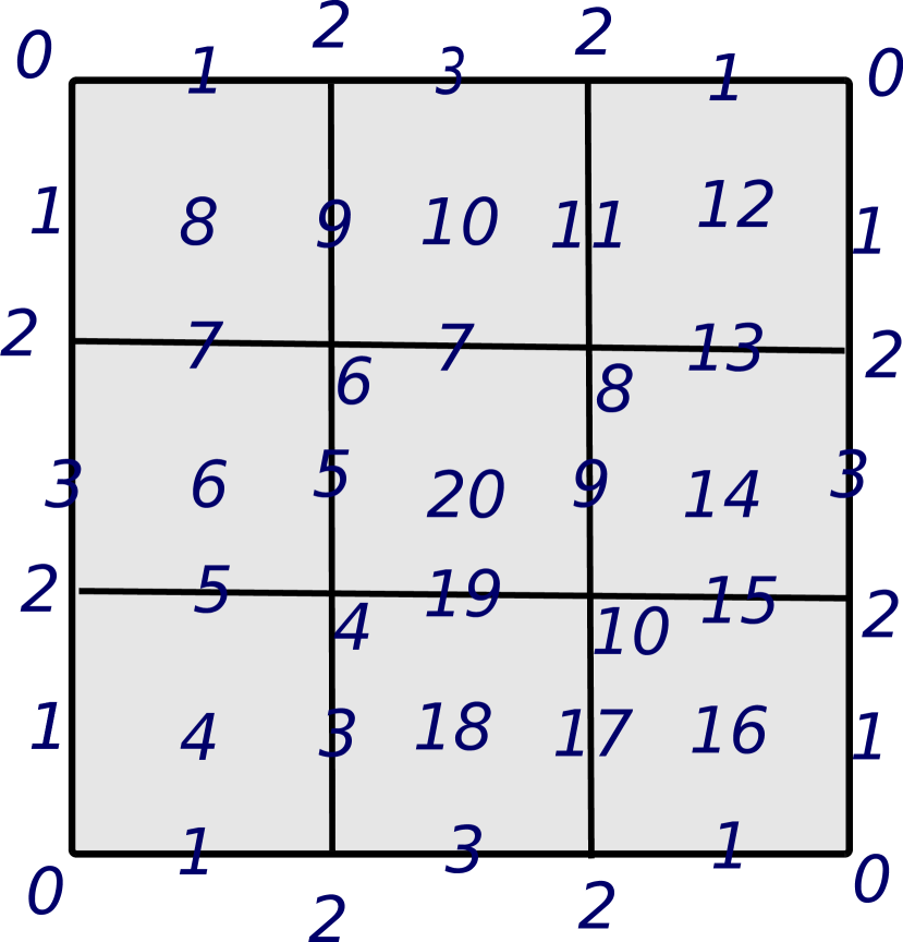
a)

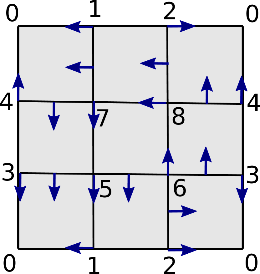
b)

Figure 1: Discrete Morse function a) and its gradient field b) on the torus

In fig. 1 shows the discrete Morse function on the torus and its gradient field. Critical cells are: 1) vertex 0, 2) edges $\{1,2\}$ and $\{3,4\}$, 3) 2- cell $[5,6,8,7]$.

The index of a critical cell (simplex) is its dimension.

The gradient path of a discrete vector field $V$ is called a sequence of cells (simplexes)

$$\tau_{0},\sigma_{1},\tau_{1},\ldots,\sigma_{m-1},\tau_{m-1},\sigma_{m}$$

such that

$$(\sigma_{i},\tau_{i})\in V,\sigma_{i}<\tau_{i-1},1\leq i\leq m,\dim\sigma_{0}=\dim\sigma_{m}.$$

Examples of gradient paths on 1 b): 1) two paths from $\{1,2\}$ to $\{0\}$ – $\{1,2\},\{1\},\{0,1\},\{0\}$ and $\{1,2\},\{2\},\{0,2\},\{0\}$; 2) two paths from $[5,6,8,7]$ to $\{1,2\}$ – $[5,6,8,7],\{5,6\},[1,2,6,5],\{1,2\}$ and $[5,6,8,7],$ $\{5,6\},$ $[1,2,6,5],\{2,6\}$,  $[2,0,3,6],\{3,6\},[6,3,4,8],\{8,4\},[8,4,0,2],\{2,8\},[8,2,1,7],\{2,1\}$.

$$\tau<\sigma\Leftrightarrow\tau\subset\sigma,\tau\neq\sigma.$$

Two discrete vector field are called isomorphic if there is an isomorphism of the CW-complexes which preserve the pairs.

Our aim is to describe all possible up to isomorphism structures of flows with one or two critical cell.

2 Discrete vector fields on the 2-disk

Since a 2-disk is homotopically equivalent to a point, any discrete gradient vector field on it will have a critical 0-cell. The optimal cellular partition of the 2-disk is a triangle - 3 vertices, 3 edges and one face (it cannot be less, since there must be at least three vertices and three edges on the boundary of the surface to fulfill the definition of a regular cellular complex). To specify discrete vector fields on a 2-disk, we use the numbering and notation of cells, as in Fig. 2.

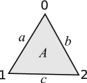
Figure 2: the numaration of cells on the 2-disk

Since the 2-cell is not critical, it belongs to one pair. Without loss of generality, we can assume that this is a pair of cA. Note that there is an axial symmetry that preserves this pair. Taking it into account, there are two possibilities for choosing a critical 0-cell: 0 or 1. In the first case, we will find such a vector field:

$$V_{1}=\{1a,2b,cA\}.$$

In the second case, the vector field is

$$V_{2}=\{0a,2b,cA\}.$$

Thus, the following is true.

Theorem 1

The number of non-isomorphic optimal discrete vector fields on the 2-disk is equal 2.

3 Discrete vector fields on the 2-sphere

According to the discrete Morse theory, an optimal discrete gradient vector field on a 2-sphere has one critical 0-cell and one critical 2-cell. An optimal regular CW-complex of a sphere has four 0-cells, six 1-cells, and four 2-cells. Let us denote the cells of the regular cell partition as shown in Fig. 3.

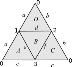
Figure 3: the numaration of cells on the 2-shpere

Without loss of generality, we assume that the critical 2-cell is cell $B$. If none of the 1-cells ($e,d,f$) bordering it are in pairs with 2-cells, then they form a cycle, which is impossible. Thus, three cases are possible: 1) one of these cells is paired with a 2-cell ($eA$), 2) two pairs ($eA$ and $fC$), 3) three pairs ($eA$, $fC$ and $dD$). In the first case, there are 2 variant:

$$V_{1-3}=\{\ldots,eA,aD,cC\},$$

$$V_{4-7}=\{\ldots,eA,aD,bC\}.$$

By $V_{1-3}$ we denote next three vector fields:

In the first variant it is possible to select the critical vertex in 3 ways (due to symmetry):

$$V_{1}=\{2b,1d,3f,eA,aD,cC\},$$

$$V_{2}=\{0b,2d,3f,eA,aD,cC\},$$

$$V_{3}=\{0b,1d,3f,eA,aD,cC\}.$$

In the second variant we have 4 vector fields:

$$V_{4}=\{1d,2f,3c,eA,aD,bC\},$$

$$V_{5}=\{0c,2d,3f,eA,aD,bC\},$$

$$V_{6}=\{0c,1d,3f,eA,aD,bC\},$$

$$V_{7}=\{0c,1d,2f,eA,aD,bC\}.$$

In the second case

$$V_{8-11}=\{\ldots,eA,fC,aD\}$$

there are four ways for critical vertex location.

In the third case

$$V_{12-13}=\{\ldots,eA,dD,fC\}$$

there are two ways for critical vertex location. Thus, the following is true.

Theorem 2

The number of non-isomorphic optimal discrete vector fields on the 2-sphere is equal 13.

4 Discrete vector fields on the cylinder

The optimal structure of the cell complex on a cylinder consists of three 2-cells, quadrilaterals, glued in a circle. All vertices in it are equal. Let’s assign number 0 to the critical vertex. We cut the cylinder along the glue, ending at this vertex. we get a rectangle divided into three squares. We number its cells as in Fig. 4.

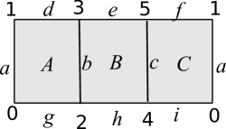
Figure 4: the numaration of cells on the cylinder

Note that an optimal vector field has one critical vertex and a critical edge. There is one non-trivial isomorphism of the cell complex onto itself, which is fixed at the critical vertex. On fig. 3 it corresponds to axial symmetry about the vertical axis.

The vector field is determined by the pairs that contain the 2-cell and the location of the critical 1-cell. The following options are possible:

$$V_{1-3}=\{\ldots,aA,bB,iC\},\ V_{4-6}=\{\ldots,aA,bB,fC\},\ V_{7-9}=\{\ldots,gA,bB,aC\},\ V_{10-12}=\{\ldots,gA,bB,iC\},$$

$$V_{13-15}=\{\ldots,gA,bB,cC\},\ \ V_{16-20}=\{\ldots,gA,bB,fC\},\ \ V_{21-23}=\{\ldots,dA,bB,aC\},$$

$$V_{24-28}=\{\ldots,dA,bB,iC\},\ \ V_{29-31}=\{\ldots,dA,bB,cC\},\ \ V_{32-34}=\{\ldots,dA,bB,fC\},$$

$$V_{35-39}=\{\ldots,gA,eB,aC\},\ \ V_{40-44}=\{\ldots,gA,eB,iC\},\ \ V_{44-49}=\{\ldots,gA,eB,cC\},$$

$$V_{50-54}=\{\ldots,gA,eB,fC\},\ \ V_{55-57}=\{\ldots,aA,eB,cC\},\ \ V_{58-60}=\{\ldots,aA,eB,fC\},$$

$$V_{61-63}=\{\ldots,bA,eB,cC\},\ \ V_{64-66}=\{\ldots,bA,eB,fC\},\ \ V_{67-69}=\{\ldots,dA,eB,fC\},$$

$$V_{70-72}=\{\ldots,gA,hB,aC\},\ \ V_{73-75}=\{\ldots,gA,hB,iC\},\ \ V_{76-78}=\{\ldots,gA,hB,cC\},$$

$$V_{79-83}=\{\ldots,gA,hB,fC\},\ \ V_{84-86}=\{\ldots,aA,hB,cC\},\ \ V_{87-91}=\{\ldots,aA,hB,fC\},$$

$$V_{92-94}=\{\ldots,bA,hB,cC\},\ \ V_{95-99}=\{\ldots,bA,hB,fC\},\ \ V_{100-104}=\{\ldots,dA,hB,fC\}.$$

Thus, the following is true.

Theorem 3

The number of non-isomorphic optimal discrete vector fields on the cylinder $S^{1}\times[0,1]$ is equal 104.

5 Discrete vector fields on the Mobius band

The case with the Mobius band is similar to the case with the cylinder. The axial symmetry of the rectangle is replaced by central symmetry. Cell designations are shown in fig. 4.

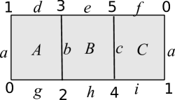
Figure 5: the numaration of cells on the Mobius band

The vector field is determined by the pairs that contain the 2-cell and the location of the critical 1-cell. The following options are possible:

$$V_{1-4}=\{\ldots,aA,bB,iC\},\ V_{5-8}=\{\ldots,aA,bB,fC\},\ V_{9-12}=\{\ldots,gA,bB,aC\},\ V_{13-16}=\{\ldots,gA,bB,iC\},$$

$$V_{17-20}=\{\ldots,gA,bB,cC\},\ \ V_{21-24}=\{\ldots,gA,bB,fC\},\ \ V_{25-28}=\{\ldots,dA,bB,aC\},$$

$$V_{29-32}=\{\ldots,dA,bB,iC\},\ \ V_{33-36}=\{\ldots,dA,bB,cC\},\ \ V_{37-40}=\{\ldots,dA,bB,fC\},$$

$$V_{41-44}=\{\ldots,gA,eB,aC\},\ \ V_{45-50}=\{\ldots,gA,eB,iC\},\ \ V_{51-54}=\{\ldots,gA,eB,cC\},$$

$$V_{55-58}=\{\ldots,gA,eB,fC\},\ \ V_{59-62}=\{\ldots,aA,eB,cC\},\ \ V_{63-66}=\{\ldots,aA,eB,iC\},$$

$$V_{58-70}=\{\ldots,aA,eB,fC\},\ \ V_{71-74}=\{\ldots,bA,eB,cC\},\ \ V_{75-78}=\{\ldots,bA,eB,iC\},$$

$$V_{79-82}=\{\ldots,bA,eB,aC\},\ \ V_{83-86}=\{\ldots,bA,eB,fC\},\ \ V_{87-90}=\{\ldots,dA,eB,aC\},$$

$$V_{91-94}=\{\ldots,dA,eB,iC\},\ \ V_{95-98}=\{\ldots,dA,eB,fC\},\ \ V_{99-102}=\{\ldots,dA,eB,cC\}.$$

Thus, the following is true.

Theorem 4

The number of non-isomorphic optimal discrete vector fields on the cylinder $S^{1}\times[0,1]$ is equal 102.

Conclusion

The results of the article prove the effectiveness of the proposed invariants (distinguishing graph and code) for classifying flows on a two-dimensional disk with one singular point. We hope that they can be used to construct similar invariants for flows with a large number of singular points on other surfaces as well.

Taras Shevchenko National University of Kyiv

Svitlana Bilun             Email address: bilun@knu.ua           Orcid ID: 0000-0003-2925-5392

Maria Hrechko              Email: mariyagr2808@gmail.com      Orcid ID: 0009-0005-5347-0342

Olena Myshnova          Email: myshnova.olena@gmail.com   Orcid ID: 0009-0001-8808-0038

Alexandr Prishlyak      Email address: prishlyak@knu.ua      Orcid ID: 0000-0002-7164-807X

References

- [1] O. Akchurin, S. Bilun, and A. Prishlyak. Three-color graph as the 1-skeleton of the 2-sphere triangulation. arXiv preprint arXiv:2209.05737, 2022. doi:10.48550/ARXIV.2209.05737.
- [2] S. Bilun and A. Prishlyak. The closed morse 1-forms on closed surfaces. Visn., Mat. Mekh., Kyv. Univ. Im. Tarasa Shevchenka, 2002(8):77–81, 2002.
- [3] S. Bilun and A. Prishlyak. Visualization of morse flow with two saddles on 3-sphere diagrams. arXiv preprint arXiv:2209.12174, 2022. doi:10.48550/ARXIV.2209.12174.
- [4] S. Bilun, A. Prishlyak, and A. Prus. Morse flows with fixed points on the boundary of 3-manifold. arXiv preprint arXiv:2209.04019, 2022. doi:10.48550/arXiv.2209.04019.
- [5] A.V. Bolsinov and A.T. Fomenko. Integrable Hamiltonian systems. Geometry, Topology, Classification. A CRC Press Company, Boca Raton London New York Washington, D.C., 2004. 724 p.
- [6] R. Forman. Morse theory for cell complexes. Advances in Mathematics. 134 (1): 90–145. 1998. doi:10.1006/aima.1997.1650.
- [7] J. Gross and T. Tucker. Topological graph theory. Wiley, 1987.
- [8] F. Harary. Graph Theory. Westview Press, 1969.
- [9] Ch. Hatamian and A. Prishlyak. Heegaard diagrams and optimal morse flows on non-orientable 3-manifolds of genus 1 and genus 2. Proceedings of the International Geometry Center, 13(3):33–48, 2020. doi:10.15673/tmgc.v13i3.1779.
- [10] P. Hilton and S. Wylie. Homology theory: An introduction to algebraic topology. Cambridge University Press, 1968.
- [11] B. I. Hladysh and A. O. Pryshlyak. Functions with nondegenerate critical points on the boundary of the surface. Ukrainian Mathematical Journal, 68(1):29–41, 2016. doi:10.1007/s11253-016-1206-5.
- [12] B.I. Hladysh and A.O. Prishlyak. Topology of functions with isolated critical points on the boundary of a 2-dimensional manifold. SIGMA. Symmetry, Integrability and Geometry: Methods and Applications, 13:050, 2017. doi:0.3842/SIGMA.2017.050.
- [13] B.I. Hladysh and A.O. Prishlyak. Simple morse functions on an oriented surface with boundary. Журнал математической физики, анализа, геометрии, 15(3):354–368, 2019. doi:10.15407/mag15.03.354.
- [14] A.S. Kronrod. Functions of two variables. Russian Mathematical Surveys, 5:24–134, 1950.
- [15] Z. Kybalko, A. Prishlyak, and R. Shchurko. Trajectory equivalence of optimal Morse flows on closed surfaces. Proc. Int. Geom. Cent., 11(1):12–26, 2018. doi:10.15673/tmgc.v11i1.916.
- [16] M. Losieva and A. Prishlyak. Topology of morse–smale flows with singularities on the boundary of a two-dimensional disk. Pr. Mizhnar. Heometr. Tsentr, 9(2):32–41, 2016. doi:10.15673/tmgc.v9i2.279.
- [17] D.P. Lychak and A.O. Prishlyak. Morse functions and flows on nonorientable surfaces. Methods of Functional Analysis and Topology, 15(03):251–258, 2009.
- [18] A.A. Oshemkov and V.V. Sharko. Classication of morse-smale flows on two-dimensional manifolds. Matem. Sbornik, 189(8):93–140, 1998.
- [19] M.M. Peixoto. On the classication of flows of 2-manifolds. Dynamical Systems (Proc. Symp. Univ. of Bahia, Salvador, Brasil, 1971), pages 389–419, 1973.
- [20] A. Prislyak and A. Prus. Morse-smale flows on torus with hole. Proc. Int. Geom. Cent., 10(1):47–58, 2017. doi:10.15673/tmgc.v1i10.549.
- [21] A.O. Prishlyak. On graphs embedded in a surface. Russian Mathematical Surveys, 52(4):844, 1997. doi:10.1070/RM1997v052n04ABEH002074.
- [22] A.O. Prishlyak. Morse–smale vector fields without closed trajectories on-manifolds. Mathematical Notes, 71(1-2):230–235, 2002. doi:10.1023/A:1013963315626.
- [23] A.O. Prishlyak. On sum of indices of flow with isolated fixed points on a stratified sets. Zhurnal Matematicheskoi Fiziki, Analiza, Geometrii [Journal of Mathematical Physics, Analysis, Geometry], 10(1):106–115, 2003.
- [24] A.O. Prishlyak. Complete topological invariants of morse–smale flows and handle decompositions of 3-manifolds. Fundamentalnaya i Prikladnaya Matematika, 11(4):185–196, 2005.
- [25] A.O. Prishlyak. Complete topological invariants of morse-smale flows and handle decompositions of 3-manifolds. Journal of Mathematical Sciences, 144:4492–4499, 2007.
- [26] A. Prishlyak and M. Loseva. Topological structure of optimal flows on the girl’s surface. Proceedings of the International Geometry Center, 15(3-4):184–202, 2022.
- [27] A. Prishlyak, A. Prus, and S. Guraka. Flows with collective dynamics on a sphere. Proc. Int. Geom. Cent, 14(1):61–80, 2021. doi:10.15673/tmgc.v14i1.1902.
- [28] A. Prishlyak and M. Loseva. Topology of optimal flows with collective dynamics on closed orientable surfaces. Proceedings of the International Geometry Center, 13(2):50–67, 2020. doi:10.15673/tmgc.v13i2.1731.
- [29] A.O. Prishlyak. Equivalence of morse function on 3-manifolds. Methods of Func. Ann. and Topology, 5(3):49–53, 1999.
- [30] A.O. Prishlyak. Conjugacy of morse functions on surfaces with values on a straight line and circle. Ukrainian Mathematical Journal, 52(10):1623–1627, 2000. doi:10.1023/A:1010461319703.
- [31] A.O. Prishlyak. Morse functions with finite number of singularities on a plane. Meth. Funct. Anal. Topol, 8:75–78, 2002.
- [32] A.O. Prishlyak. Topological equivalence of morse–smale vector fields with beh2 on three-dimensional manifolds. Ukrainian Mathematical Journal, 54(4):603–612, 2002.
- [33] A.O. Prishlyak. Topological classification of m-fields on two-and three-dimensional manifolds with boundary. Ukrainian Mathematical Journal, 55(6):966–973, 2003.
- [34] A.O. Prishlyak and M.V. Loseva. Optimal morse–smale flows with singularities on the boundary of a surface. Journal of Mathematical Sciences, 243:279–286, 2019.
- [35] A.O. Prishlyak and K.I. Mischenko. Classification of noncompact surfaces with boundary. Methods of Functional Analysis and Topology, 13(01):62–66, 2007.
- [36] A.O. Prishlyak and A.A. Prus. Three-color graph of the morse flow on a compact surface with boundary. Journal of Mathematical Sciences, 249(4):661–672, 2020. doi:10.1007/s10958-020-04964-1.
- [37] G. Reeb. Sur les points singuliers d’une forme de pfaff complétement intégrable ou d’une fonction numérique. C.R.A.S. Paris, 222:847—849, 1946.
- [38] V.V. Sharko. Functions on manifolds. Algebraic and topological aspects., volume 131 of Translations of Mathematical Monographs. American Mathematical Society, Providence, RI, 1993.
- [39] S. Smale. On gradient dynamical systems. Ann. of Math., 74:199–206, 1961.
- [40] В.М. Кузаконь, В.Ф. Кириченко, and О.О. Пришляк. Гладкi многовиди. Геометричнi та топологiчнi аспекти. Працi Iнcтитуту математики НАН України.—2013.—97.—500 с, 2013.
- [41] А.О. Пришляк. Векторные поля Морса–Смейла с конечным числом особых траекторий на трехмерных многообразиях. Доповiдi НАН України, (6):43–47, 1998.
- [42] А.О. Пришляк. Сопряженность функций Морса. Некоторые вопросы совр. математики. Институт математики АН Украины, Киев, 1998.
- [43] А.О. Пришляк. Топологическая эквивалентность функций и векторных полей Морса—Смейла на трёхмерных многообразиях. Топология и геометрия. Труды Украинского мат. конгресса, pages 29–38, 2001.
- [44] А.О. Пришляк. Векторные поля Морса–Смейла без замкнутых траекторий на трехмерных многообразиях. Математические заметки, 71(2):254–260, 2002.
- [45] О.О. Пришляк. Топологiя многовидiв. Київський унiверситет, 2015.