Topological phase transitions generated by order from quantum disorder

Abstract

The order from quantum disorder (OFQD) phenomenon was first discovered in quantum spin systems in geometric frustrated lattice. Similar phenomenon was also discovered in interacting bosonic systems or quantum spin systems with spin-orbit coupling in a bipartite lattice. Here we show that the OFQD also leads to a topological phase transition. We demonstrate this new connection in the experimentally realized weakly interacting Quantum Anomalous Hall system of spinor bosons in an optical lattice. There are two classes of topological phenomena: the first class is a perturbative one smoothly connected to the non-interacting limit. The second one is a non-perturbative one which has no analog in the non-interacting limit. Their experimental detections are also discussed.

1. Introduction. — Searching for new topological phases and topological phase transitions in various materials or artificial systems are fascinating frontiers in modern condensed matter physics kane ; zhang . The quantum anomalous Hall (QAH) is the simplest topological phase with non-vanishing Chern number QAHthe . The non-interacting fermionic QAH has been experimentally realized in Cr doped Bi(Sb)₂Te₃ thin films QAHthe ; QAHexp . On the other hand, the weakly interacting bosonic analogy of QAH model has also been successfully realized via spinor bosons ⁸⁷Rb 2dsocbec . It is crucial to study the topological properties of bosonic QAH model, and find possible deep connections between the fermionic QAH model and the bosonic QAH model.

It is well-known that the fermionic QAH model has two bands carrying opposite Chern numbers. In the non-interacting limit, when $|h/t|<4$, the corresponding Chern number of the lower and upper band are $C_{1}=+\mathrm{sgn}(h)$ and $C_{2}=-\mathrm{sgn}(h)$, respectively; when $|h/t|>4$, the corresponding Chern number of the lower and upper bands is $C_{1}=C_{2}=0$. However, the topological properties of weakly interacting bosonic quantum anomalous Hall model maybe much involved. Due to its bosonic nature, an interaction must be considered at the very beginning. Unlike the fermionic QAH model, the weakly interacting bosonic QAH model is always in some spin-orbital superfluid phases with the spontaneous U(1) symmetry breaking. To the quadratic level, there are always Bogliubov quasi-particle excitations above these exotic superfluid phases. If neglecting the cubic or quartic interactions between them, which is justified near any quantum phase transitions (QPT), one may ask the question on what are the topology of these Bogliubov quasi-particle bands and possible TPTs. In this Letter, we map out the Chern number of the bosonic Bogliubov band at the quadratic level.

In Ref.NOFQD , we work out quantum phases and quantum phase transitions in NOFQD . It is the order from quantum disorder (OFQD) phenomena which leads to the quantum ground states at $h=0$. It is the nearly order from quantum disorder (NOFQD) phenomena which leads to the quantum phase transition at $h=h_{c}$. In this work, we focus on the topological aspects of the same system. So the results to be achieved are complementary to those achieved in NOFQD . We find that there are two kinds of topological phases and TPTs. The first can be considered as the remnants from the non-interacting fermion limit, so it reduce to this limit smoothly as the interaction gets very small. It can also be called perturbative regime. The second has no analog or counterpart in the non-interacting fermion limit, so it is a completely new feature due to the interaction. We will show that it is completely induced by the non-perturbative OFQD phenomenon at $h=0$ discovered in NOFQD . It may also be called perturbative regime.

In addition to the OFQD at $h=0$ and the QPT at $h=h_{c}$ induced by the NOFQD discovered in NOFQD , we find two critical fields $h_{2}>h_{1}>h_{c}>0$. At the upper critical field $h=h_{2}$, there is a conic band touching at the $R=(\pi,\pi)$ point of the Brillouin zone (BZ), so the lower band $C_{1}$ and upper band $C_{2}=-C_{1}$ Chern number changes from $(C_{1},C_{2})=(+1,-1)$ below $h_{2}$ to $(C_{1},C_{2})=(0,0)$ above $h_{2}$; At the lower critical field $h_{1}<h_{2}$, there is a conic band touching at the $X=(\pi,0)$ and $Y=(0,\pi)$ point of the BZ, so $(C_{1},C_{2})=(-1,+1)$ changes below $h_{1}$ to $(C_{1},C_{2})=(+1,-1)$ above $h_{1}$. Both $h_{1}$ and $h_{2}$ only depends on $t$ and $U$, but independent of the SOC $t_{s}$, and approaches to the corresponding non-interacting value $h_{20}=4t$ and $h_{10}=0$ respectively. We conclude the topology in the regime $|h|>|h_{1}|$ belongs to the first perturbative class.

We show that $h=h_{1}>h_{c}$ which is due to the NOFQD NOFQD . When $h<h_{c}$, the ground state becomes a XY-CAFM SF phase which breaks $[C_{4}\times C_{4}]_{D}\to 1$ and leads to 4 bosonic Bogliubov bands in the reduced BZ. We find there is always a gap between the second and the third band and calculate the combined Chern numbers of the two lower bands and that of the two upper bands $(C_{1+2},C_{3+4})=(-1,+1)$. So there is no change on the topological band structure across the QPT at $h=h_{c}$. However, the change comes from $h=0$ where the OFQD leads to two Dirac points at in-commensurate momenta. Their positions not only depend on $t,U$, but also the SOC $t_{s}$ and related by the remaining two Mirror symmetries. As the three parameters change, the two Dirac points approach to each other, then collide at a degenerate momentum $\Lambda=(\pi/2,\pi/2)$, then bounce off along the normal direction. Any $h\neq 0$ opens the gap on the two Dirac points, so there is a TPT from $h<0$ with the combined Chern number $(C_{1+2},C_{3+4})=(1,-1)$ to $h>0$ with $(C_{1+2},C_{3+4})=(-1,1)$, which is completely induced by the OFQD at $h=0$. We construct effective action to study the TPT and find it always contains an exotic Doppler shift term. The topology in the regime $|h|<|h_{1}|$ belongs to the second non-perturbative class. We also critically comment on the common conceptual mistakes made in the previous theoretical or experimental literatures to attempt to evaluate edge modes within the bulk gaps associated with the bosonic bulk Chern numbers. We also elucidate the physical meanings of the combined Chern numbers. Finally, we discuss the experimental detection of these topological phenomena, especially the ones induced by the OFQD near $h=0$.

2. The Hamiltonian, quantum phases and quantum phase transitions (QPT). — The recently experimentally realized two-component spinor Bose-Hubbard Hamiltonian with a spin-orbit coupling 2dsocbec can be written as

$$\mathcal{H}=-\!\sum_{i}[a_{i}^{\dagger}(t\sigma_{z}\!-\!it_{\text{s}}\sigma_{x})a_{i+x}\!+\!a_{i}^{\dagger}(t\sigma_{z}\!-\!it_{\text{s}}\sigma_{y})a_{i+y}\!+\!h.c.]$$

$$\qquad-h\sum_{i}(n_{i\uparrow}-n_{i\downarrow})+U\sum_{i}n^{2}_{i}-\mu\sum_{i}n_{i}\>.$$ (1)

where $\sigma=\uparrow$ or $\downarrow$ denotes the ⁸⁷Rb atoms in the state $|1,m_{F}=0\rangle$ or $|1,m_{F}=-1\rangle$, respectively. Since the experiment can only achieve relatively weak spin-orbit coupling, our discussion will focus on regime $|t_{s}|<2|t|$.

The quantum phase diagram of Eq.(1) was studied in Ref.NOFQD . Especially, we found a new phenomenon we named Nearly order from quantum disorder (NOFQD) which captures the delicate competition between the effective potential generated by the order from quantum disorder (OFQD) and the Zeeman field. It is this competition which splits a putative first order quantum phase transition (QPT) at $h=0$ into two second order QPTs at $h=\pm h_{c}$. Here we briefly summarize the main results: when $h>h_{c}$, it is in the Z-FM superfluid with the condensate wavefunction $\Psi\propto\chi_{\uparrow}$; when $h<h_{c}$, it is the XY-CAFM superfluid with the condensate wavefunction $\Psi\propto\cos(\theta/2)\chi_{\uparrow}+e^{i(\mathbf{Q}\cdot\mathbf{r}+\phi)}\sin(\theta/2)\chi_{\downarrow}$, where $\mathbf{Q}=(\pi,\pi)$ is the orbital ordering wave-vector, $\theta=\arccos(h/h_{c})$, and $\phi=\pm\pi/4,\pm 3\pi/4$. The $h_{c}$ was estimated as $h_{c}\sim n_{0}U^{2}t_{s}^{2}/t^{3}$.

However, Ref.NOFQD fucus only on the quantum phases and QPTs, ignored the topological features of the Bogoliubov bands, also did not touch what are the connections of these quantum phases and QPTs to the topological nature of the QAH Hamiltonian. This work will address these outstanding open problems. Without loss of generality, we can set $h,t,t_{\text{s}}>0$ and then discuss the topology of the Bogoliubov excitation bands at $h>h_{c}$ and $h<h_{c}$ separately.

3. Evaluating the Chern number of the bosonic quasi-particle band from the lattice theory. — To exam the topology of the Bogoliubov excitation bands, we need not only the eigenvalues but also the eigenvectors, thus one need also to pay attention to the Bogoliubov transformations. After replacing the bosonic operator by its average plus a quantum fluctuation, we obtain a quadratic Bogoliubov Hamiltonian via expanding the Hamiltonian to the second order in the quantum fluctuations. Due to the spontaneous U(1) symmetry breaking, the quadratic Hamiltonian in $\mathbf{k}$-space, $H_{\mathbf{k}}$, is a $2N\times 2N$ matrix,

$$\mathcal{H}=E_{0}+\frac{1}{2}\sum_{\mathbf{k}}(\psi_{\mathbf{k}}^{\dagger},\psi_{-\mathbf{k}})H_{\mathbf{k}}\begin{pmatrix}\psi_{\mathbf{k}}\\ \psi_{-\mathbf{k}}^{\dagger}\\ \end{pmatrix}\>,$$ (2)

where $\psi_{\mathbf{k}}^{\dagger}\!=\!(\psi_{1,\mathbf{k}}^{\dagger},\cdots,\psi_{N,\mathbf{k}}^{\dagger})$. The $1,\cdots,N$ indices count the spin degrees of freedom and also the momentum resulting from the spontaneous translational symmetry breaking i9n the ground state. As shown in NOFQD , when $h>h_{c}$, the ground state is the Z-FM phase, we have $N=2$ and $\psi_{\mathbf{k}}^{\dagger}=(\psi_{\mathbf{k}\uparrow}^{\dagger},\psi_{\mathbf{k}\downarrow}^{\dagger})$; when $h<h_{c}$, the ground state is the XY-AFM phase, we have $N=4$ and $\psi_{\mathbf{k}}^{\dagger}=(\psi_{\mathbf{k}\uparrow}^{\dagger},\psi_{\mathbf{k}\downarrow}^{\dagger},\psi_{\mathbf{k}+\mathbf{Q}\uparrow}^{\dagger},\psi_{\mathbf{k}+\mathbf{Q}\downarrow}^{\dagger})$. where $\vec{Q}=(\pi,\pi)$.

Diagonalizing Eq.(2) by a $2N\times 2N$ Bogoliubov transformation matrix $T_{\mathbf{k}}$, so that $T_{\mathbf{k}}^{\dagger}H_{\mathbf{k}}T_{\mathbf{k}}=\mathrm{diag}(\omega_{1,\mathbf{k}},\cdots,\omega_{N,\mathbf{k}},\omega_{1,-\mathbf{k}},\cdots,\omega_{N,-\mathbf{k}})$ where $\mathrm{diag}(\cdots)$ means a diagonal matrix with diagonal elements $\cdots$, and $(\begin{smallmatrix}\psi_{\mathbf{k}}\\ \psi_{-\mathbf{k}}^{\dagger}\\ \end{smallmatrix})=T_{\mathbf{k}}(\begin{smallmatrix}\alpha_{\mathbf{k}}\\ \alpha_{-\mathbf{k}}^{\dagger}\\ \end{smallmatrix})$, we obtain

$$\mathcal{H}=E_{0}+\sum_{n,\mathbf{k}}\omega_{n,\mathbf{k}}(\alpha_{n,\mathbf{k}}^{\dagger}\alpha_{n,\mathbf{k}}+1/2),$$ (3)

where $\mathbf{k}$ sums over the corresponding Brillouin Zone (BZ), $\omega_{n,\pm\mathbf{k}}>0$, $n=1,\cdots,N$ are the $N$ Bogoliubov excitation bands.

In contrast to the fermionic cases, to keep the bosonic commutation relations, the $T_{\mathbf{k}}$ is required to be a para-unitary matrix instead of a unitary one, which means $T_{\mathbf{k}}^{\dagger}\tau_{3}T_{\mathbf{k}}=T_{\mathbf{k}}\tau_{3}T_{\mathbf{k}}^{\dagger}=\tau_{3}$ and $\tau_{3}=\sigma_{z}\otimes I_{N\times N}$. The Berry curvature of the $n$-th Bogoliubov excitation band can be calculated via $F_{n}(\mathbf{k})=i[\epsilon_{\mu\nu}\tau_{3}\partial_{\mu}T_{\mathbf{k}}^{\dagger}\tau_{3}\partial_{\nu}T_{\mathbf{k}}]_{nn}$, where $\mu,\nu=k_{x},k_{y}$. The Chern number of the $n$-th Bogoliubov excitation band can be evaluated via a integral

$$C_{n}=\frac{1}{2\pi}\int_{\text{BZ}}d^{2}\mathbf{k}\>F_{n}(\mathbf{k})\>,$$ (4)

where the integral is over the corresponding BZ.

4. Evaluating the Chern number of the bosonic quasi-particle band from the continuum theory. — Since the band closing is the signature of a topological phase transition (TPT), the change of band Chern number may also be computed in terms of a continuum theory.

Near the band touching point, the typical effective Hamiltonian can be expressed in terms of the polar coordinate $(k,\xi)$ with $k_{x}=k\cos\xi$ and $k_{y}=k\sin\xi$,

$$H_{\mathbf{k}}=v_{x}k^{n}\cos(n\xi)\sigma_{x}+v_{y}k^{n}\sin(n\xi)\sigma_{y}-\Delta\sigma_{z}$$ (5)

where $|v_{x}|=|v_{y}|=v$ and $n=1,2,3,\cdots$ stands for the order ( or charge ) of the touching point.

The corresponding dispersion relation is $\epsilon(\mathbf{k})=\pm\sqrt{\Delta^{2}+v^{2}k^{2n}}$, and $\epsilon(\mathbf{k})\sim k^{n}$ as $\Delta\to 0$ approaching the TPT. The Berry curvature of the lower branch is $F_{-}(\mathbf{k})=-v_{x}v_{y}\Delta k^{-2+2n}n^{2}/|\epsilon(k)|^{3}$, thus its Chern number is

$$C_{-}=\frac{1}{2\pi}\int d^{2}\mathbf{k}F_{-}(\mathbf{k})=-\frac{n}{2}\mathrm{sgn}(v_{x}v_{y}\Delta)\>.$$ (6)

where the $sgn$ indicates the chirality of the Dirac boson. Therefore the band touching through the changing sign of $\Delta$ from positive to negative across the TPT leads to a change of Chern number $\Delta C_{=}-n\,\mathrm{sgn}(v_{x}v_{y})$. When there are multiple band touching points, the total change of Chern number needs to sum up all the contributions from all the band touching points.

In the superfluid phases, due to the BEC at $k=0$, the Bogoliubov transformation matrix $T_{k}$ diverges at $k=0$, the Chern number of the lowest band $C_{1}$ may not be well-defined, but those of the higher bands $C_{n>1}$ are usually well-defined, and quantized to be integers. Ueda2015 . In this Letter, we are still able to calculate $C_{1}$ by excluding the momentum $k$ where the BEC resides. The results are summarized in Fig. 1. When comparing the non-interacting fermionic QAH model with the interacting bosonic QAH model, we find that the bosonic interaction leads to new and additional patterns of topological bands. In the following sections, we present the details of calculations leading to Fig.1.

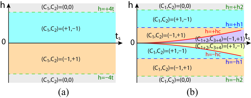
Figure 1: The band Chern numbers of (a) The non-interacting fermionic QAH, and (b) The weak-interacting bosonic QAH. The topological non-trivial regions ($C_{i}\neq 0$) in (b) is slightly larger than (a). The regime $|h|>h_{1}$ region is smoothly connected to the non-interacting limit in (a), so can be called perturbative region. While the entire $|h|<h_{1}$ region is induced by the non-perturabative OFQD phenomenon at $h=0$. It has no non-interacting analog, so may be called the non-perturabative region which shrinks to zero as $U$ goes $0$.

5. The topology of the Bogoliubov band when $h>h_{c}$.— In the $h>h_{c}$ case, the ground state is the Z-FM phase, there are $N=2$ energy bands, the Bogoliubov transformation matrix $T_{k}$ is a $4\times 4$ matrix. The corresponding band structure is plotted in Fig.2 where

$$h_{2} =\sqrt{4t(4t+n_{0}U)}$$

$$h_{1} =\sqrt{2t(2t+n_{0}U)}-2t$$ (7)

When $h=h_{2}$, the two bands conically touch at $k_{R}=(\pi,\pi)$; when $h=h_{1}$, they conically touch at $k_{X}=(\pi,0)$ and $k_{Y}=(0,\pi)$. A direct evaluation of Eq.(4) on the lattice shows that: when $h>h_{2}$, the lower band and the upper band Chern number are $C_{1}=C_{2}=0$ respectively; when $h_{1}<h<h_{2}$, $(C_{1},C_{2})=(1,-1)$; when $h<h_{1}$, $(C_{1},C_{2})=(-1,1)$. Below, we construct continuum theories to confirm the change of the band Chern number.

At $h=h_{2}$, one needs to expand the Hamiltonian around $k_{R}=(\pi,\pi)$, the $T_{k}$ at $k_{R}$ tells the eigenmodes are $\alpha_{1,R}=(1/\sqrt{8})[2(4+n_{0}U/t)^{-1/4}+(4+n_{0}U/t)^{1/4}]\psi_{R\uparrow}-(1/\sqrt{8})[2(4+n_{0}U/t)^{-1/4}-(4+n_{0}U/t)^{1/4}]\psi_{R\uparrow}^{\dagger}$ and $\alpha_{2,R}=\psi_{R\downarrow}$, with the eigen-energy $\omega_{h2}\!=\!2\sqrt{\smash[b]{4t(4t\!+\!n_{0}U)}}=2h_{2}$ When $h$ deviates slightly from $h_{2}$, defining $k=k_{R}+q$ and projecting the original Hamiltonian onto these eigenmodes lead to the effective Hamiltonian:

$$H_{R}=\omega_{h2}-vq_{x}\sigma_{x}-vq_{y}\sigma_{y}-\Delta\sigma_{z}$$ (8)

where $omega_{h2}\!=2h_{2},\Delta=2(h-h_{2})$, $v\!=\!t_{\text{s}}\sqrt{\smash[b]{2[1\!+\!(8t\!+\!n_{0}U)/\omega_{h2}\!]}}$. Note that the constant term $omega_{h2}$ shows it is an excited energy which has a direct experimental consequence CIT .

Then the dispersion takes the form

$$\omega_{1,2}(q)=\omega_{h2}\mp\sqrt{\Delta^{2}+v^{2}(q_{x}^{2}+q_{y}^{2})}\>.$$ (9)

Thus the change of band Chern number is $\Delta C_{1}=-{\rm sgn}(v^{2})=-1$. This analysis is consistent with the numerical result $C_{1}=0$ at $h>h_{2}$ and $C_{1}=+1$ at $h<h_{2}$, therefore $0-(+1)=-1$.

At $h=h_{1}$, one needs to expand the Hamiltonian around $k_{X}=(\pi,0)$ and $k_{Y}=(0,\pi)$, the $T_{k}$ at $k_{X}$ and $k_{Y}$ tells the eigenmodes are $\alpha_{1,X(Y)}=(1/\sqrt{8})[2(2+n_{0}U/t)^{-1/4}+(2+n_{0}U/t)^{1/4}]\psi_{X(Y)\uparrow}-(1/\sqrt{8})[2(2+n_{0}U/t)^{-1/4}-(2+n_{0}U/t)^{1/4}]\psi_{X(Y)\uparrow}^{\dagger}$ and $\alpha_{2,X(Y)}=\psi_{X(Y)\downarrow}$, with the eigen-energy $\omega_{h1}\!=\!2\sqrt{\smash[b]{2t(2t\!+\!n_{0}U)}}=2h_{1}+4t$. When $h$ deviates slightly from $h_{1}$, defining $k=k_{X(Y)}+q$ and projecting the original Hamiltonian onto these eigenmodes lead to the effective Hamiltonian

$$H_{X} =\omega_{h1}-vq_{x}\sigma_{x}+vq_{y}\sigma_{y}-\Delta\sigma_{z}$$

$$H_{Y} =\omega_{h1}+vq_{x}\sigma_{x}-vq_{y}\sigma_{y}-\Delta\sigma_{z}$$ (10)

where $\omega_{h1}\!=2h_{1}+4t,\Delta=2(h-h_{1})$, $v\!=\!t_{\text{s}}\sqrt{\smash[b]{2[1\!+\!(4t\!+\!n_{0}U)/\omega_{h1}\!]}}$. Again, the constant term $omega_{h2}$ shows it is an excited energy which has a direct experimental consequence CIT .

Then the dispersion of $H_{X}$ or $H_{Y}$ takes the same form

$$\omega_{1,2}(q)=\omega_{h1}\mp\sqrt{\Delta^{2}+v^{2}(q_{x}^{2}+q_{y}^{2})}\>.$$ (11)

Thus the change of band Chern number is $\Delta C_{1}=2{\rm sgn}(v^{2})=2$. This analysis is consistent with the numerical result $C_{1}=+1$ at $h>h_{1}$ and $C_{1}=-1$ at $h<h_{1}$, therefore $+1-(-1)=2$.

Since $\lim_{U\to 0}h_{2}=4t$ and $\lim_{U\to 0}h_{1}=0$, this result suggests that the topology of the Bogoliubov excitation bands at $h>h_{c}$ is smoothly connecting to that of the non-interacting limit. Besides, the fact $h_{2}=\sqrt{4t(4t+n_{0}U)}>4t$ at any $U>0$ suggests that the region displaying a non-trivial topology ( with a non-zero Chern number) is enlarged with an increasing $U>0$.

One can also determine the relation between $h_{1}$ and $h_{c}$ when $U/t$ is small. When $U/t$ is small, $h_{1}=\sqrt{2t(2t+n_{0}U)}-2t\sim n_{0}U/2$, while $h_{c}\sim n_{0}U^{2}t_{s}^{2}/t^{3}\ll h_{1}$. Thus in the weak coupling limit $U/t\ll 1$, there is always a window for $h_{c}<h<h_{1}$ as shown in Fig.1b.

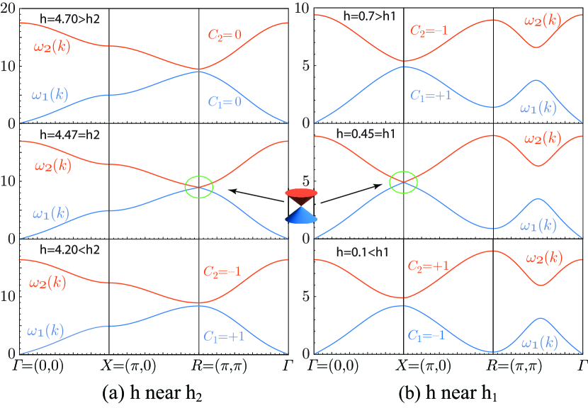
Figure 2: The perturbative topological band structure of Bogoliubov excitation bands at $h>h_{c}$ and near (a) $h_{2}$ and (b) $h_{1}$. It is smoothly connected to the non-interacting limit. The parameters are $t=1$, $t_{s}=1/2$, $n_{0}U=1$, thus $h_{2}\approx 4.47$ and $h_{1}\approx 0.48$. When $h=h_{2}$, there is a Dirac conical band touch at the R point $k_{R}=(\pi,\pi)$ of the Brillouin zone (BZ). When $h=h_{1}$, there is a Dirac conical band touch at the X point $k_{X}=(\pi,0)$ of the BZ. The $[C_{4}\times C_{4}]_{\text{diag}}$ symmetry tells there is also a Dirac conical band touch at the Y point $k_{Y}=(0,\pi)$ of the BZ.

6. The topology of the Bogoliubov band when $0<h<h_{c}$ and the absence of the TPT across the QPT at $h=h_{c}$.— In the $h<h_{c}$ case, this corresponds to Eq.(9) and Eq.(10) in Ref.NOFQD . Because of spontaneous translational symmetry breaking, we have $N=4$ energy bands and $T_{k}$ is an $8\times 8$ matrix. From the NOFQD analysis in Ref.NOFQD , we know the $h=0$ ground-state requires $\theta=\pi/2$, and $0<h<h_{c}$ ground-state requires $\theta_{h}=\arccos(h/h_{c})$. We substitute $\theta=\theta_{h}$ back into the Eq.(2), then calculate the band Chern numbers via Eq.(4). In principle, there should be an additional term due to nearly order-from-quantum disorder (NOFQD) correction NOFQD , but we expect this correction does not change the topology of the Bogoliubov bands. From the band structure shown in Fig.3, we find that the two lower bands touch, the two upper bands also touch, and there is always a band gap between the two groups when decreasing $\theta_{h}$ from $\pi/2$ to $0$ (or equivalently, increasing $h$ from $0$ for $h_{c}$). Note that two lower/upper bands touch at the X point $k_{X}=(\pi,0)$, which is a momentum far away from $k=0$, thus the NOFQD effects ignored so far should not change the band touching behaviors. Due to the band touching, we need to consider the combination of the Chern numbers $C_{1+2}$ and $C_{3+4}$ when $h<h_{c}$. Our numerical evaluation of the integral Eq.(4) gives $(C_{1+2},C_{3+4})=(-1,+1)$. Recall the result of $h$ just above $h_{c}$ achieved in the last subsection also gives $(C_{1},C_{2})=(-1,+1)$, which is the same pattern as $(C_{1+2},C_{3+4})=(-1,+1)$. So we conclude that there is not any change in the topology across the quantum phase transition at $h=h_{c}$.

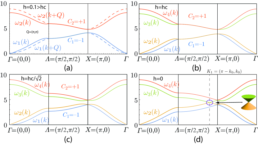
Figure 3: The Non-perturbative band structure of Bogoliubov excitation bands at (a) $h>h_{c}$, (b) $h=h_{c}$, (c) $h=h_{c}/\sqrt{2}$, (d) $h=0$. The parameters are $t=1$, $t_{s}=1/2$, $n_{0}U=1$. It has no analog in the non-interacting limit. When $h>0$, there is always a band gap between two upper bands and two lower bands. (a) is just a re-plot of the bottom subfigure of Fig.2(b) in the reduced Brillouin zone (BZ), so the 2 bands in the BZ changes to 4 bands in the reduced BZ. As shown in Sec.C in the SM, two lower (upper) bands also touch along the whole line from $(\pi,0)$ to $(0,-\pi)$ As shown in (a) and (b), when $h\geq h_{c}$, they also touch along the whole line from $\Lambda$-point to the X-point along the boundary of the RBZ. $\omega_{1}$ is the linear gapless Goldstone mode due to the $U(1)$ symmetry breaking. Note that due to the dropping of the NOFQD effects NOFQD , the roton mode $\omega_{1}$ is still a spurious quadratic gapless mode at $k=0$. Incorporating them back will open a small roton gap at $k=0$, but will not change the Chern numbers of topology of the band. When $h=0$ in (d), there is a Dirac conical band touch at $K_{1}=(\pi-k_{0},k_{0})$ of Brillouin zone; and the mirror symmetry $M_{1}$ with respect to $k_{x}=k_{y}$ tells there is also a Dirac conical band touch at $K_{2}=(k_{0},\pi-k_{0})$.

7. The TPT at $h=0$ and the absence of any QPT at $h=0$. — As shown in Fig.2, the topology changes at $h=h_{1}$ with the conic band crossings at $k_{X}=(\pi,0)$ and $k_{Y}=(0,\pi)$, also at $h=h_{2}$ with the conic band crossing at $k_{R}=(\pi,\pi)$. The origin of these TPTs can be traced back and mapped to the corresponding non-interacting limit of fermions.

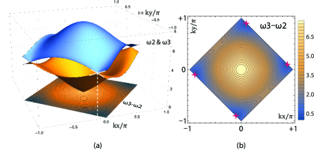
Figure S2: The OFQD induced band structure of Bogoliubov excitation bands $\omega_{2}$ and $\omega_{3}$ at $h=0$. The parameters are $t=1$, $t_{s}=1/2$, $n_{0}U=1$, and $\theta=\pi/2$, $\phi=-\pi/4$. The bottom plane is the contour plot of $\omega_{3}-\omega_{2}$ as a function of $k_{x}$ and $k_{y}$. It is clear to see there are two Dirac points at the two in-commensurate momenta denoted by $+$ sitting on the Reduced BZ boundary.

In this section, we show that there is also a conic band crossing at $h=0$ in Fig.3(d) at some in-commensurate momentum $(k_{0x},k_{0y})$ between the $\Lambda$-point and X-point, which is not any high symmetry points. As shown in Fig.S2, there are two such Dirac points in the RBZ. The positions of the two Dirac points are in-commensurate and also depend on $t,t_{s}$ and $U$, so it comes from the interaction induced OFQD NOFQD . In contrast to the TPTs at $h=h_{1}$ and $h=h_{2}$, the TPT at $h=0$ does not have any non-interacting analog.  sl This is also the cental result achieved in this manuscript .

At $h=0$, the ground state wavefunction is the XY-AFM with $\theta=0$ and $\phi=-\pi/4$. Solving the band-touching condition $\omega_{2}(k)=\omega_{3}(k)$ leads to the following three cases: (I) when $n_{0}U/t<8t_{s}/(\sqrt{2}t-t_{s})$, two solutions are $K_{1}=(\pi-k_{0},k_{0})$ and $K_{2}=(k_{0},\pi-k_{0})$, with $k_{0}=\arcsin[\sqrt{2}tn_{0}U/(t_{s}(8t+n_{0}U))]<\pi/2$; (II) when $n_{0}U/t>8t_{s}/(\sqrt{2}t-t_{s})$, two solutions are $P_{1,2}=\pm(p_{0},p_{0})$, with $p_{0}=\arcsin[(4t/(8t+n_{0}U))\sqrt{4t(4t+n_{0}U)/(4t^{2}-2t_{s}^{2})}]<\pi/2$; (III) when $n_{0}U/t=8t_{s}/(\sqrt{2}t-t_{s})$, the two solutions merge into just one at $\Lambda=(\pi/2,\pi/2)$. Intuitively, as shown in Fig.S2, when keeping $h=0$, increasing $n_{0}U/t$ from $0^{+}$ to $8t_{s}/(\sqrt{2}t-t_{s})$, the $\omega_{2,3}$ conically touch at $K_{1,2}$; then at $n_{0}U/t=8t_{s}/(\sqrt{2}t-t_{s})$, $K_{1}$ and $K_{2}$ collide at $\Lambda$-point; further increasing $n_{0}U/t$, they bounce off along the two opposite directions along the perpendicular direction footnote , so $\omega_{2,3}$ conic touches at $P_{1,2}$.

Around $h=0$, defining $k=K_{1,2}+q$ or $k=P_{1,2}+q$, we can similarly expand the Hamiltonian around the two minima of $\omega_{2,3}$ to find the effective Hamiltonian:

$$H_{1}=\omega_{0}+c_{\parallel}q_{\parallel}+v_{\parallel}q_{\parallel}\sigma_{x}+v_{\perp}q_{\perp}\sigma_{y}\!-\Delta\sigma_{z}\>,$$

$$H_{2}=\omega_{0}-c_{\parallel}q_{\parallel}-v_{\parallel}q_{\parallel}\sigma_{x}-v_{\perp}q_{\perp}\sigma_{y}\!-\Delta\sigma_{z}\>,$$ (12)

where $\omega_{0}=8t(4t+n_{0}U)/(8t+n_{0}U)$, $q_{\parallel}=(q_{x}-q_{y})/\sqrt{2},q_{\perp}=(q_{x}+q_{y})/\sqrt{2}$, and $\Delta=hn_{0}U\sqrt{t/(4t+n_{0}U)}$ for regime (I), $q_{\parallel}=(q_{x}+q_{y})/\sqrt{2},q_{\perp}=(q_{x}-q_{y})/\sqrt{2}$, and $\Delta=4htt_{s}/\sqrt{2t^{2}-t_{s}^{2}}$ for regime (II). The effective velocities $v_{\parallel},v_{\perp},c_{\parallel}>0$ are proportional to $\cos(k_{0})$ or $\cos(p_{0})$ for regime (I) and regime (II) respectively and are listed in the appendix B.

The dispersion of $H_{i},i=1,2$ takes the form

$$\omega_{2,3}(q)=\omega_{0}-(-1)^{i}c_{\parallel}q_{\parallel}\mp\sqrt{\Delta^{2}+v_{\parallel}^{2}q_{\parallel}^{2}+v_{\perp}^{2}q_{\perp}^{2}}\>.$$ (13)

It is necessary to stress that there exists a Doppler shift term, the $c$ term, in $H_{1,2}$, which is the salient feature unique to the OFQD induced TPT, not shared by any non-interacting counter-part. Of course, it does not affect the value of band Chern numbers.

From the effective Hamiltonian Eq.(12), Eq.(6) tells the change of band Chern number is $\Delta C=-2{\rm sgn}(v_{\parallel}v_{\perp})=-2$ when $\Delta$ changes from positive to negative. This result is consistent with the numerical evaluation via Eq.(4), which gives $C_{1+2}=-1$ at $h>0$ and $C_{1+2}=+1$ at $h<0$, therefore $-1-(+1)=-2$.

At $h=0$, in the colliding point $n_{0}U/t=8t_{s}/(\sqrt{2}t-t_{s})$, the $K_{1}$ and $K_{2}$ merge at $\Lambda=(\pi/2,\pi/2)$-point. Expanding around the $\Lambda$-point leads to the dispersion:

$$\omega_{2,3}(q)=\omega_{0}(q)\mp\sqrt{u_{1}^{2}q^{4}_{\perp}+u_{2}q^{4}_{\parallel}+wq^{2}_{\parallel}q^{2}_{\perp}},$$ (14)

where $u_{1}=t^{2}/(\sqrt{2}t_{s})$, $u_{2}=t^{2}t_{s}/[\sqrt{2}(2t^{2}-t_{s}^{2})]$, $w=t^{2}(t^{2}-t_{s}^{2})/(2t^{2}-t_{s}^{2})$, and $\omega_{0}(q)=4t+2\sqrt{2}t_{s}+DS$ where one can see the Doppler shift term $DS=[t_{s}/\sqrt{2}][-q^{2}_{\parallel}+q^{2}_{\perp}t_{s}^{2}/(2t^{2}-t_{s}^{2})]$ also gets to the quadratic order.

Note that $4u_{1}^{2}u_{2}^{2}>w^{2}$ is ensured by the condition $0<t_{s}<\sqrt{2}t$, so the square root is always positive define. Since $w$-term won’t lead to a gap close, one can ignore $w$-term and rescale $q$ to make $\omega_{2,3}(q)$ isotropic. The $\omega_{2,3}(q)\sim q^{2}$ is consistent with the fact that $v_{\parallel}$, $v_{\perp}$, $c_{\parallel}$ in Eq.(12) vanish as $k_{0}$ or $p_{0}$ approaching $\pi/2$. When $h$ deviates from $0$, the effective Hamiltonian belongs to $n=2$ case of Eq.(5). Thus, although there is only one band touching point with the monopole charge $n=2$, the change of Chern number is still $-2$.

In short, regardless of the value of $n_{0}U$, the change of the Chern number from $h=0^{+}$ to $h=0^{-}$ is always $-2$. So the scattering process in Fig. S1, is not a TPT.

8. Dramatic differences between the non-interacting fermionic band structure and the bosonic Bogoliubov band structure at the quadratic level.— It is important to stress some crucial differences between the fermionic band structure and the bosonic Bogliubov band structure at the quadratic level and also pointed out the common mistakes made in all the previous literatures to calculate the edge modes associated with the bosonic Bogliubov band structure:

In the fermionic or bosonic QAH problem, the Time reversal symmetry is broken, the Chern number is not protected by any symmetry, its definition involves no symmetry requirement. The former is really non-interacting, while the bosonic Bogoliubov band is non-interacting at the quadratic level only where one dropped the cubic and quartic interactions and all the higher order interactions. All these interactions are not important except near the QPT at $h=h_{c}$. In fact, as shown by the RG analysis, near the QPT, the two quartic interaction in Eq.M32 are marginally irrelevant. But both are relevant inside the XY-AFM phase and in fact, leads to the symmetry breaking inside the phase.

For the fermionic problem, there are always edge states associated with the topological phases. This is justified, because a single fermion operator never condenses. One tempts to also calculate the edge modes within the band gaps in Fig.2 and Fig.3 associated with the bosonic Bogoliubov band. Unfortunately, this kind of calculation has mathematical meanings, but makes no physical sense: this is because Eq.M3 is based on the BEC at $k=0$ in the Z-FM phase, Eq.M9 with the parametrization Eq. M11 are based on the BEC at both $k=0$ and $Q=(\pi,\pi)$ in the XY-AFM phase. Unfortunately, they are ill-defined in a strip geometry. Ref.Ueda2015 and many other previous works, just copied the same method from its fermionic counterpart to evaluate edge modes associated with the bosonic Bogoliubov band: They simply transfer the quadratic Bogoliubov band in momentum space to real space, then solve the edge modes in the strip geometry by putting a periodic boundary condition along one direction, then the open boundary condition along the other. Unfortunately, this approach is well-planned mathematically, but is not self-consistent physically, because it ignored the root of BEC which leads to the quadratic bands in the first place. As stressed above, the BEC root is ill-defined in the strip geometry. So it makes no physical sense to talk about the edge modes. The claims made in some experimental works to measure the edge modes have no physical grounds.

9. Experimental detections.— So far, the experiment2dsocbec has detected the non-interacting fermionic Chern numbers Fig.1a using the highly excited bosonic spinors, so it just mimic the single particle properties of the Hamiltonian Eq.1 using a spinor boson with SOC. Its main purpose is to demonstrate a possible realization of the bosonic Hamiltonian Eq.1 using cold atoms. The common drawbacks of most cold atom experiments is just to demonstrate a possibility to simulate a Hamiltonian which has been well studied in materials and claim the ability to tune the parameters. But in reality, it is rare to go beyond just a simulation to demonstrate new many-body phenomenon or topological phenomena due to many-body interactions..

Here we showed that there are two kinds of topological band structures (1) The one in the regime $|h|>|h_{1}|$ is smoothly connected to the non-interacting fermionic one. So it can also be called perturbative regime. Even so, the two critical fields $h_{1,2}$ listed in Eq.7 still depends on the interaction $n_{0}U$. All the parameters in the effective Hamiltonian Eq.8 and 10 also depend on the interaction $n_{0}U$. (2) The one in the regime $-h_{1}<h<h_{1}$ has no analog in the non-interacting counter-part, so it is completely due to the many-body interaction. More specifically, due to the non-perturbative OFQD. So it can also be called non-perturbative regime. It is also an experimentally easily accessible regime in the cold atom systems.

It is extremely important to push the already 6 year old experiment2dsocbec beyond the single-particle picture: to detect this novel purely interaction induced topological phenomena. In contrast to the detections suggested in NOFQD which are all equilibrium properties in the ground states and low energy excitations, here are the excited states near the high energy $\omega_{h2},\omega_{h1}$ and $\omega_{0}$ in Eq.8,10 and 12 near the high momentum $R=(\pi,\pi)$ or $X=(\pi,0),Y=(0,\pi)$ and tunable in-commensurate momenta $K_{1,2}$ or $P_{1,2}$ respectively CIT . We suggest to also measure the scattering process of the two bosonic Dirac points at $h=0$ displayed in Fig.S1 by the Bragg spectroscopy becbragg ; bragg1 ; bragg2 or the momentum resolved interband transitions mrit adapted to the excited states.

10. Conclusions.— For any interacting Hamiltonian with a non-trivial topology in the non-interacting limit such as the QAH one Eq.1, there are always two aspects quantum and topology. The former focus on the ground states and quantum phase transitions which may only depend on the low energy excitations around the band minima in the weak interaction limit. OFQD is needed to even determine the ground state. NOFQD is needed to determine the QPT at $h=h_{c}$. The latter focus on the global structure of the bands, therefore also the excited states to capture the global topology CIT . However, the Bogliubov quasi-particle band picture breaks down near the QPT near $h=h_{c}$ where a RG analysis is needed to capture all the physics well beyond the quadratic band picture.

However, as classified in NOFQD , there are two kinds of OFQD, the first response trivially to a deformation, no NOFQD phenomenon emerging from the OFQD. The second response highly non-trivially to a deformation and lead to NOFQD phenomenon. It would be interesting to see if there are also two classes here, the first leads to a TPT, as is the case presented in this work, the second does not lead to any TPT. The two criterions coincide in the present case. It is also worthy to see if the two criterions coincide in other cases.

The OFQD and the topological invariants such as Chern number seem are two very different concepts. The first concept is a completely many-body quantum phenomenon. While the latter is mainly a non-interacting topological phenomenon. Here we show that there are deep connections between the two in the context of the experimentally realized weakly interacting Quantum Anomalous Hall system of spinor bosons in an optical lattice. We expect this new effects could also be realized in frustrated quantum spin systems which leads to topological phase transitions of magnons.

Acknowledgements

J. Ye thanks Prof. Gang Tian for the hospitality during his visit at the School of Science of Great Bay University.

In this Supplemental Materials we provide some details of the band structures which are needed to construct the effective Hamiltonian near the various TPTs.

I A. Symmetry analysis and the scattering process of the two bosonic Dirac points at $h=0$

The high symmetry points in the 1st Brillouin zone are defined as

$$\Gamma=(0,0),~{}\Lambda=(\pi/2,\pi/2),~{}R=(\pi,\pi),~{}X=(\pi,0),~{}Y=(0,\pi).$$ (S1)

Two additional special $k$-points are defined as the band minima ( maxima ) of $\omega_{3}(k)$ ( $\omega_{2}(k)$ ) when $|h|<h_{c}$, they are functions of spin-orbit coupling $t_{s}$ and the interaction $U$.

At $h=0$, if the interaction strength $U$ is sufficiently small $n_{0}U/t<8t_{s}/(\sqrt{2}t-t_{s})$, the $\omega_{3}(k)$ has two minima at $k=K_{1}=(\pi-k_{0},k_{0})$ and $k=K_{2}=(k_{0},\pi-k_{0})$, where

$$k_{0}=\arcsin\Big{[}\frac{\sqrt{2}tn_{0}U}{t_{s}(8t+n_{0}U)}\Big{]}\>.$$ (S2)

When $n_{0}U$ goes to $0$, the $k_{0}$ will become $0$, thus $K_{1}$ becomes $X$-point and $K_{2}$ becomes $Y$-point.

At $h=0$, if the interaction strength $U$ is relatively large $n_{0}U/t>8t_{s}/(\sqrt{2}t-t_{s})$, the $\omega_{3}(k)$ has two minima at $k=P_{1}=(+p_{0},+p_{0})$ and $k=P_{2}=(-p_{0},-p_{0})$, where

$$p_{0}=\arcsin\Big{[}\frac{4t}{8t+n_{0}U}\sqrt{\frac{4t(4t+n_{0}U)}{4t^{2}-2t_{s}^{2}}}\Big{]}$$ (S3)

At $h=0$, if $n_{0}U/t=8t_{s}/(\sqrt{2}t-t_{s})$, the $\omega_{3}(k)$ has only one minima at $k=\Lambda=(\pi/2,\pi/2)$ with the monopole charge $n=2$.

In summary, pictorially as illustrated in Fig.S1, at $h=0$, increasing $n_{0}U$ from $0^{+}$ to the value greater than $8tt_{s}/(\sqrt{2}t-t_{s})$, the two minima of $\omega_{3}(k)$ approach each other along the line $k_{0x}+k_{0y}=\pi$, then collide at $\Lambda$-point, then the two minima bounce off along the opposite direction along the perpendicular direction $k_{0x}=k_{0y}$.

The point group symmetry of the square lattice is $C_{4v}$. In the presence of spin-orbit coupling, the $C_{4v}$ symmetry becomes $[C_{4}\times C_{4}]_{\text{diag}}$ symmetry, which is a joint 4-fold rotation of spin and orbit. Besides, there are also two mirror symmetries $M_{1,2}$, which also inherit from the $C_{4v}$ point group symmetry. The mirror symmetry $M_{1}$ is a composition of time reversal $i\to-i,\vec{\sigma}\to-\vec{\sigma}$, the orbit reflection $k_{x}\leftrightarrow k_{y}$, and the spin rotation $(\sigma_{x},\sigma_{y},\sigma_{z})\to(\sigma_{y},\sigma_{x},-\sigma_{z})$. The mirror symmetry $M_{2}$ is a composition of the orbit reflection $\vec{k}\to-\vec{k}$, and the spin rotation $(\sigma_{x},\sigma_{y},\sigma_{z})\to(-\sigma_{x},-\sigma_{y},\sigma_{z})$.

When $h>h_{c}$, the ground state is the Z-FM superfluid phase where both $[C_{4}\times C_{4}]_{\text{diag}}$ and $M_{1,2}$ symmetries are unbroken.

When $h<h_{c}$, it is the XY-CAFM superfluid where the $[C_{4}\times C_{4}]_{\text{diag}}\to 1$ is broken while $M_{1,2}$ remain unbroken. It is the $M_{1}$ symmetry which guarantees the two minima $K_{1}=(k_{0},\pi-k_{0})$ and $K_{2}=(\pi-k_{0},k_{0})$ are related by $k_{x}\leftrightarrow k_{y}$. It is the $M_{2}$ symmetry which guarantees the two minima $P_{1}=(+p_{0},+p_{0})$ and $P_{2}=(-p_{0},-p_{0})$ are related by $k\leftrightarrow-k$. The colliding point $\Lambda=(\pi/2,\pi/2)$ is the mirror symmetric point which is invariant under both $M_{1}$ and $M_{2}$.

It is constructive to compare the mirror symmetric point $\Lambda=(\pi/2,\pi/2)$ in the momentum space here with that in the SOC parameter space $\beta=\pi/2$ discussed in SOCM . In the former, the Hamiltonian which is the sum over all momenta has the same symmetry, the Doppler shit term still exists at a quadratic order, but non-vanishing. While in the latter, the Hamiltonian has an enlarged symmetry which dictates the exact vanishing of the Doppler shift term.

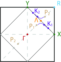
Figure S1: Illustration of the special k-points used in this Letter: $\Gamma=(0,0),~{}\Lambda=(\pi/2,\pi/2),~{}R=(\pi,\pi),~{}X=(\pi,0),~{}Y=(0,\pi)$. The $K_{1}$ and $K_{2}$ are the two minima of $\omega_{3}(k)$ when $n_{0}U/t<8t_{s}/(\sqrt{2}t-t_{s})$; the $P_{1}$ and $P_{2}$ are the two minima of $\omega_{3}(k)$ when $n_{0}U/t>8t_{s}/(\sqrt{2}t-t_{s})$. The arrows show that: as $n_{0}U/t$ increases, the two minima of $\omega_{3}(k)$ approach each other along the X-Y line, then collide at $\Lambda$-point, then bounce off into two opposite perpendicular directions. The thick square is the lattice Brillouin Zone (BZ), the thin one is the reduce Brillouin Zone (RBZ).

It is interesting to compare the scattering process of the two bosonic Dirac points with the same chirality in Fig.S1 with the annihilation process of the two fermionic Dirac points with the opposite chirality discussed in TQPT . As shown in this work, the former happens in the high energy modes, so it is not a QPT. It is not a TPT either. While the latter is both where various physical quantities satisfy various scaling functions. The collision of two bosonic vortices with opposite vorticities in an expanding curved space-time was analyzed in gravity where two surface waves also emerge after the collision and head in opposite direction along the normal direction.

II B. Determination of the band structures induced by the OFQD at $h=0$.

Solving the band touching condition $\omega_{2}(k)=\omega_{3}(k)$ within the regime (I) $n_{0}U/t<8t_{s}/(\sqrt{2}t-t_{s})$, we obtain the two solutions $K_{1}=(k_{0x},k_{0y})$ and $K_{2}=(k_{0y},k_{0x})$, where

$$k_{0y}=\arcsin\Big{[}\frac{\sqrt{2}tn_{0}U}{t_{s}(8t+n_{0}U)}\Big{]}=k_{0},\quad k_{0x}=\pi-k_{0}.$$ (S4)

The two solutions are related by the remaining $M_{1}$ symmetry. The band touching happened at high energy $\omega_{2}(K_{1})=\omega_{3}(K_{1})=8t(4t+n_{0}U)/(8t+n_{0}U)=\omega_{0}>4t$. Expanding the $\omega_{2,3}(k)$ near $K_{1,2}$ with $k=K_{1,2}+q$, we obtain

$$\omega_{2,3}(K_{1}+q)=\omega_{0}\mp\sqrt{v_{1}^{2}(q_{x}-q_{y})^{2}+v_{2}^{2}(q_{x}+q_{y})^{2}}+c(q_{x}-q_{y})\>,$$

$$\omega_{2,3}(K_{2}+q)=\omega_{0}\mp\sqrt{v_{1}^{2}(q_{x}-q_{y})^{2}+v_{2}^{2}(q_{x}+q_{y})^{2}}-c(q_{x}-q_{y})\>,$$ (S5)

where

$$v_{1} =\sqrt{2}\cos k_{0}\,t_{s}(8t+n_{0}U)/\sqrt{\smash[b]{16t(4t+n_{0}U)}},$$

$$v_{2} =\sqrt{2}\cos k_{0}\,t_{s}(8t+n_{0}U)^{2}/[16t(4t+n_{0}U)],$$

$$c =\sqrt{2}\cos k_{0}\,t_{s}n_{0}^{2}U^{2}/[16t(4t+n_{0}U)].$$ (S6)

The two solutions are related by the remaining $M_{1}$ symmetry. The Doppler shift term is along the $[1\bar{1}]$ direction, which is nothing but the “collision” direction in Fig.S1. Note that the relative sizes of $v_{1}$ and $c$ is not important here, due to the high energy $\omega_{0}$ which has direct experimental consequences as stressed in Sec.M9, so it will not drive any instabilities. In a sharp contrast, in the fermionic QAH under an injecting current discussed in QAHinj , due to the absence of the $\omega_{0}$ term, the sign change of the relative size drives a TPT.

Solving the band touching condition $\omega_{2}(k)=\omega_{3}(k)$ within the regime (II) $n_{0}U/t>8t_{s}/(\sqrt{2}t-t_{s})$, we obtain the two solutions $P_{1}=+(k_{0x},k_{0y})$ and $P_{2}=-(k_{0x},k_{0y})$, where

$$k_{0x}=k_{0y}=\arcsin\Big{[}\frac{4t}{8t+n_{0}U}\sqrt{{\frac{4t(4t+n_{0}U)}{4t^{2}-2t_{s}^{2}}}}\Big{]}=p_{0}.$$ (S7)

The two solutions are related by the remaining $M_{2}$ symmetry. The band touching happens at the high energy $\omega_{2}(P_{1})=\omega_{3}(P_{1})=8t(4t+n_{0}U)/(8t+n_{0}U)=\omega_{0}>4t+2\sqrt{2}t_{s}$. Expanding the $\omega_{2,3}(k)$ near $P_{1,2}$ with $k=P_{1,2}+q$, we obtain

$$\omega_{2,3}(P_{1}+q)=\omega_{0}\mp\sqrt{v_{1}^{2}(q_{x}+q_{y})^{2}+v_{2}^{2}(q_{x}-q_{y})^{2}}+c(q_{x}+q_{y})\>,$$

$$\omega_{2,3}(P_{2}+q)=\omega_{0}\mp\sqrt{v_{1}^{2}(q_{x}+q_{y})^{2}+v_{2}^{2}(q_{x}-q_{y})^{2}}-c(q_{x}+q_{y})\>,$$ (S8)

where

$$v_{1} =[2t(8t+n_{0}U)/(n_{0}U)]\cot p_{0},$$

$$v_{2} =[t_{s}(8t+n_{0}U)/\sqrt{8t(4t+n_{0}U)}]\cos p_{0},$$

$$c =[2tn_{0}U/(8t+n_{0}U)]\cot p_{0}$$ (S9)

The Doppler shift term is along the $[11]$ direction, which is nothing but the “bouncing-off” direction in Fig.S1.

In summary, near the band touching point, we always have

$$\omega_{2,3}(K_{i}+q\text{ or }P_{i}+q)=\omega_{0}\mp\sqrt{\smash[b]{v_{\parallel}^{2}(q_{\parallel})^{2}+v_{\perp}^{2}(q_{\perp})^{2}}}-(-1)^{i}c_{\parallel}q_{\parallel}\>,$$ (S10)

where $i=1,2$, $q_{\parallel}=(q_{x}-q_{y})/\sqrt{2},q_{\perp}=(q_{x}+q_{y})/\sqrt{2}$ for regime (I), $q_{\parallel}=(q_{x}+q_{y})/\sqrt{2},q_{\perp}=(q_{x}-q_{y})/\sqrt{2}$ for regime (II), and $v_{\parallel},v_{\perp},c_{\parallel}$ are easy to deduce from the previous expressions Eq.S6 and Eq.S9.

III C. The folding of the two lower bands and the two upper bands and the physical meanings of $C_{I}=C_{1+2}$ and $C_{I\!I}=C_{3+4}$ at $h<h_{c}$.

Now we look at the band structures of the two lower bands and the two upper bounds. At $h=0$, in the XY-AFM phase with $c_{0}=1/\sqrt{2}$ and $c_{\pi}=e^{-i\pi/4}/\sqrt{2}$, solving the band touching condition $\omega_{1}(k)=\omega_{2}(k)$ or $\omega_{3}(k)=\omega_{4}(k)$, we find the solutions $k=(k_{0x},k_{0y})$ form a straight line $\{(k_{0x},k_{0y})|k_{0x}-k_{0y}=\pi\}$. Thus, there is a line degeneracy between $\omega_{1}$ and $\omega_{2}$. The Fig.S3 shows that the $\omega_{1}$ and $\omega_{2}$ indeed touch along one reduced BZ edge.

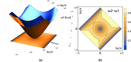
Figure S3: The band structure of the Bogoliubov excitation bands $\omega_{1}$ and $\omega_{2}$ at $h=0$. The bottom plane is the contour plot of $\omega_{2}-\omega_{1}$ as a function of $k_{x}$ and $k_{y}$. It is clear to see the two bands merge along one reduced BZ edge from $(0,-\pi)$ to $(\pi,0)$. The parameters are the same as Fig.S2.

The line degeneracy between $\omega_{1,2}$ and $\omega_{3,4}$ suggests that we can unfold the two bands along $[1\,\bar{1}]$ direction, by defining $\Omega_{I}(k)=\omega_{2}(k)$ if $k$ in reduced BZ, otherwise $\Omega_{I}(k)=\omega_{1}(k+Q^{\prime})$ where $Q^{\prime}=(+\pi,-\pi)$. Similarly, we define $\Omega_{I\!I}(k)=\omega_{3}(k)$ if $k$ in the reduced BZ, otherwise $\Omega_{I\!I}(k)=\omega_{4}(k+Q^{\prime})$.

The unfolded band structures are plotted in Fig.S4. Thus it is more nature to consider $\omega_{1,2}$ as one band and $\omega_{3,4}$ as the other band; this is the physical reason we always consider a combination of band Chern numbers $C_{I}=C_{1+2}$ and $C_{I\!I}=C_{3+4}$.

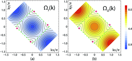
Figure S4: The unfold Bogoliubov excitation bands $\Omega_{I}$ and $\Omega_{I\!I}$ at $h=0$. There are two conic band crossings between $\Omega_{I}$ and $\Omega_{I\!I}$. The green dashed line represents the reduce Brillouin zone. The new Brillouin zone is a rectangular shape, and the two Dirac points denoted by $+$ sit on the longer side. The parameters are the same as Fig.S2. When adding a small $0<|h|<h_{c}$, the line degeneracy still exists, so $\Omega_{I}(k)$ and $\Omega_{I\!I}(k)$ are still well-defined. Due to the symmetry $[C_{4}\times C_{4}]_{D}$ restoration of the Z-FM above $h>h_{c}$, the line degeneracy remains. Of course, any small $h$ opens a gap between $\Omega_{I}$ and $\Omega_{I\!I}$ around the two Dirac points and Lead to the two effective Hamiltonians Eq.M13.

References

• (1) M. Z. Hasan and C. L. Kane, Colloquium: Topological insulators, Rev. Mod. Phys. 82, 3045 (2010).
• (2) X. L. Qi and S. C. Zhang, Topological insulators and superconductors, Rev. Mod. Phys. 83, 1057 (2011).
• (3) Rui Yu, Wei Zhang, Hai-Jun Zhang, Shou-Cheng Zhang, Xi Dai1, Zhong Fang, Quantized Anomalous Hall Effect in Magnetic Topological Insulators, Science 329, 61 (2010).
• (4) Cui-Zu Chang, Jinsong Zhang, Xiao Feng, Jie Shen, Zuocheng Zhang, Minghua Guo1, Kang Li, Yunbo Ou, Pang Wei, Li-Li Wang, Zhong-Qing Ji, Yang Feng1, Shuaihua Ji, Xi Chen, Jinfeng Jia1, Xi Dai2, Zhong Fang2, Shou-Cheng Zhang3, Ke He2,?, Yayu Wang1,?, Li Lu2, Xu-Cun Ma2, Qi-Kun Xue1, Experimental Observation of the Quantum Anomalous Hall Effect in a Magnetic Topological Insulator, Science 340, 167 (2013).
• (5) Zhan Wu, Long Zhang, Wei Sun, Xiao-Tian Xu, Bao-Zong Wang, Si-Cong Ji, Youjin Deng, Shuai Chen, Xiong-Jun Liu, Jian-Wei Pan, Realization of two-Dimensional spin-orbit coupling for Bose-Einstein condensates, Science 354, 83 (2016).
• (6) Fadi Sun and Jinwu Ye, Nearly order from quantum disorder phenomena, arXiv:1903.11134, substantially revised version.
• (7) Shunsuke Furukawa1 and Masahito Ueda, Excitation band topology and edge matter waves in Bose-Einstein condensates in optical lattices, New J. Phys. 17 (2015) 115014.
• (8) Si-Cong Ji, Long Zhang, Xiao-Tian Xu, Zhan Wu, Youjin Deng, Shuai Chen, and Jian-Wei Pan, Softening of Roton and Phonon Modes in Bose-Einstein Condensate with Spin-Orbit Coupling, Phys. Rev. Lett. 114, 105301 (2015).
• (9) Jinwu Ye, J.M. Zhang, W.M. Liu, K.Y. Zhang, Yan Li, W.P. Zhang, Light scattering detection of various quantum phases of ultracold atoms in optical lattices, Phys. Rev. A 83, 051604 (R) (2011).
• (10) Jinwu Ye, K.Y. Zhang, Yan Li, Yan Chen and W.P. Zhang, Optical Bragg, atom Bragg and cavity QED detections of quantum phases and excitation spectra of ultracold atoms in bipartite and frustrated optical lattices, Ann. Phys. 328 (2013), 103-138.
• (11) Tarruell, L., Greif, D.,Uehlinger, T., Jotzu, G.Esslinger, T. Creating, moving and merging Dirac points with a Fermi gas in a tunable honeycomb lattice. Nature 483, 302 (2012).
• (12) Our calculations are only valid in the regime $t_{s}/t<\sqrt{2}$ and $n_{0}U/t$ below the SF-MI transition. If we fix $t_{s}$ to be some typical value between 0 and $\sqrt{2}t$, i.e. $t=1$ and $t_{s}=1/2$, then $8t_{s}/(\sqrt{2}t-t_{s})\approx 4.38$, while the typical $(U/t)_{c}$ in the Bose Hubbard model at $n=1$ for the SF-MI is about $16$. Thus both (I) and (II) are reachable in teh SF phase.
• (13) Fadi Sun, Yu Yi-Xiang, Jinwu Ye and WuMing Liu, A new universal ratio in random matrix theory and Chaotic to integral transition in type-I and type-II hybrid Sachdev-Ye-Kitaev models, Fadi Sun, Yu Yi-Xiang, Jinwu Ye, and W. M. Liu, Phys. Rev. B 104, 235133 (2021). Here, the Chaotic to integral transition (CIT) also happens in the excited bulk states which is not a QPT which involves only ground state and low energy excitations.
Supplemental Materials: Topological phase transitions induced by order from quantum disorder

References

• (1) Fadi Sun, Xiao-Lu Yu, Jinwu Ye, Heng Fan, W. M. Liu, Topological Quantum Phase Transition in Synthetic Non- Abelian Gauge Potential: Gauge Invariance and Experimental Detections, Scientific Reports 3, 2119 (2013).
• (2) Fadi Sun, Jinwu Ye, Wu-Ming Liu, Quantum incommensurate skyrmion crystals and commensurate to in-commensurate transitions in cold atoms and materials with spin–orbit couplings in a Zeeman field, New J. Phys. 19, 083015 (2017).
• (3) Fadi Sun and Jinwu Ye, Topological phase transitions, invariants and enriched bulk-edge correspondences in fermionic gapless systems with extended Fermi surface, arXiv. Long version 45 PRB page.
• (4) J. Ye and R. Bradenberger, The Formation and evolution of vortices in an expanding universe, Mod.Phys.Lett A, 157 (1990). The formation and evolution of U(1) gauged vortices in an expanding universe, Nucl. Phys. B346, 149 (1990).