Multilevel Skeletonization Using Local Separators

Abstract

In this paper we give a new, efficient algorithm for computing curve skeletons, based on local separators. Our efficiency stems from a multilevel approach, where we solve small problems across levels of detail and combine these in order to quickly obtain a skeleton. We do this in a highly modular fashion, ensuring complete flexibility in adapting the algorithm for specific types of input or for otherwise targeting specific applications.

Separator based skeletonization was first proposed by Bærentzen and Rotenberg in [ACM Tran. Graphics’21], showing high quality output at the cost of running times which become prohibitive for large inputs. Our new approach retains the high quality output, and applicability to any spatially embedded graph, while being orders of magnitude faster for all practical purposes.

We test our skeletonization algorithm for efficiency and quality in practice, comparing it to local separator skeletonization on the University of Groningen Skeletonization Benchmark [Telea’16].

1 Introduction

A curve skeleton is a compact simplified representation of a shape, consisting only of curves. The act of skeletonization, in this context, is the computation of such a curve skeleton for a given input. For the remainder of this paper skeleton refers exclusively to curve skeletons. Various fields, including feature extraction, visualisation and medical imaging, care not only about shapes and objects, but also about their structures and features. In applications such as shape matching, the skeleton acts as a simplified representation of an object, allowing for reduced computation cost [8], whereas in virtual navigation the curve skeleton can act as a collision free navigational structure [24, 30].

The broad areas of application, and the different roles that skeletons play, lead to differing interpretations of exactly what the skeleton is. Although no widely agreed upon definition of skeletons exist, work has been done on narrowing down desirable properties of skeletons in the general case [11].

Figure 1: Shaded renders of triangle meshes and skeletons obtained by our algorithm.

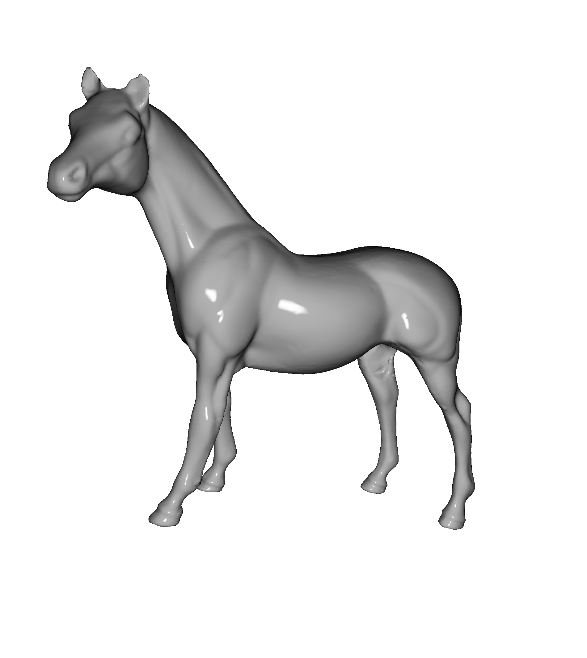
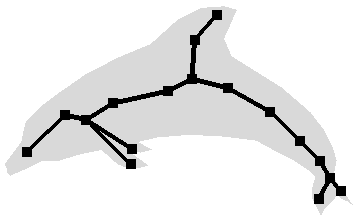
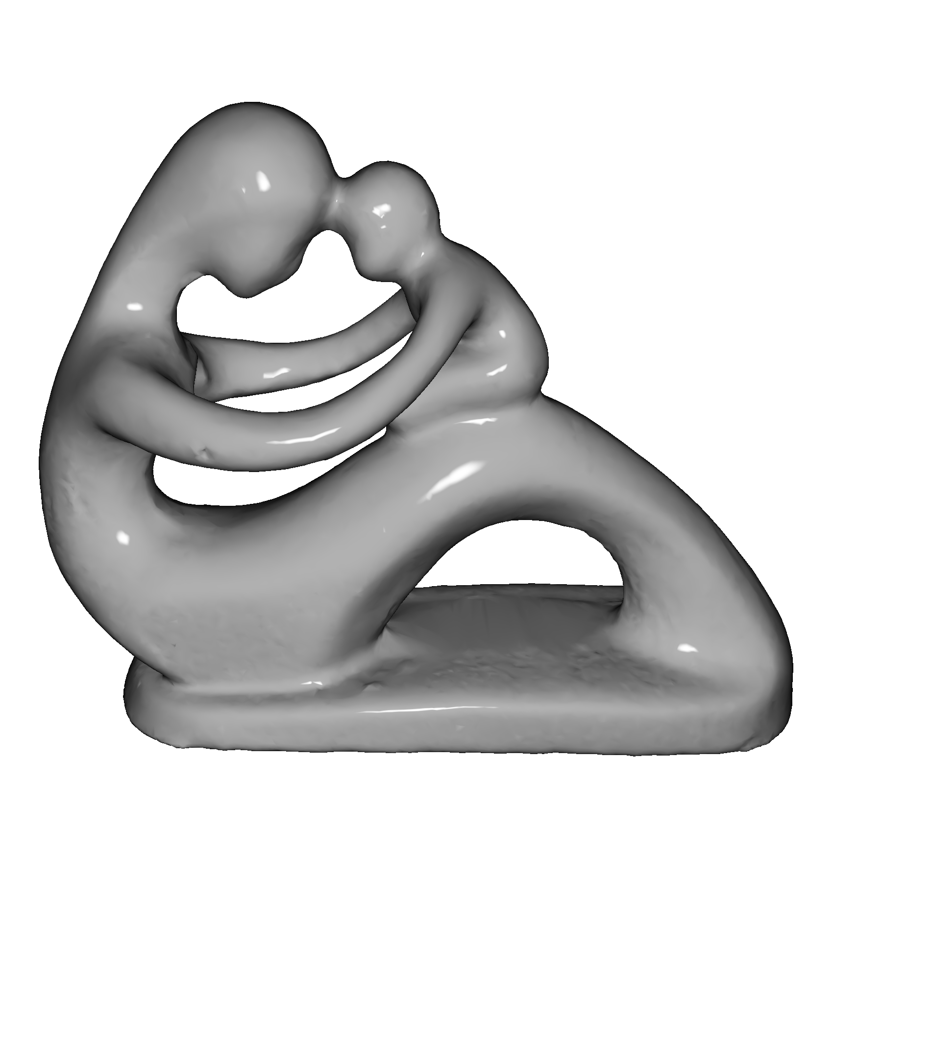
Instead of giving a formal definition, we will base our work on the evocative if imprecise definition of skeletons as simplified curve representations of the underlying structure and topology. In Figure 1 we show skeletons of various input, to exemplify our definition.

Many different approaches to skeletonization exist [27], such as computing and pruning the medial surface [12], computing mean curvature flow [26] or contracting meshes [20]. In a recent paper A. Bærentzen and E. Rotenberg present a new algorithm that bases itself on computing local separators [5]. We refer to this algorithm as the local separator skeletonization algorithm, LSS. This approach has the benefit that it requires only that the input be given as a spatially embedded graph, rather than a specific shape representation. This makes the method applicable to a wide variety of inputs, such as meshes, voxel grids or even input that does not necessarily represent a shape. In addition, the skeletons that it generates are of high quality, capturing features that contractive methods tend to miss. However, the algorithm is also computationally expensive.

In this paper we present a multilevel algorithm for computing curve skeletons that we obtain by adapting LSS to a multilevel framework. Below, we start with some preliminaries and then present an overview of our contributions. Next, after a discussion of related work, we describe our approach to graph coarsening, projecting separators onto finer level graphs, and, finally, the multilevel skeletonization algorithm that builds on these components. We provide analyses of the algorithms in the paper and we test our work on a skeletonization benchmark. Our results show that our algorithm is orders of magnitude faster than that proposed by Bærentzen and Rotenberg while producing skeletons of comparable quality.

1.1 Preliminaries

We consider the discrete skeletonization problem, where both the input and output is represented by spatially embedded undirected graphs. Formally, we consider skeletonization of a graph $G=(V,E)$ where each vertex is associated with a geometric position $p_{v\in V}\in\mathbb{R}^{3}$. Note that we make no other assumptions about the graph, such as whether it is sampled from the surface of a manifold, created from a point cloud, or otherwise.

In graph theory a vertex separator is a set of vertices whose removal disconnects the graph. In [5], this notion is extended to local separators, defined as a subset of vertices, $S\subset V$, that is a vertex separator of the subgraph induced by the closed neighbourhood of $S$. Likewise, the notion of a minimal local separator is defined as a local separator that is a minimal vertex separator of the subgraph induced by the closed neighbourhood. Intuitively, we cannot remove a vertex from a minimal local separator without the remaining set ceasing to be a local separator. For the rest of this paper, the term separator means local separator.

1.2 Contributions

The LSS algorithm computes skeletons through a three-phased approach. A large number of minimal local separators is computed, the minimal separators are selected using a greedy packing method, and, lastly, the skeleton is extracted from the packed set of minimal separators. A visualisation of these phases can be seen in Figure 2.

Figure 2: Visualisation of the three phases of the LSS algorithm. From left to right: A shaded render of the input, a number of computed minimal separators, a non-overlapping subset of the separators, and the resulting skeleton after extraction.

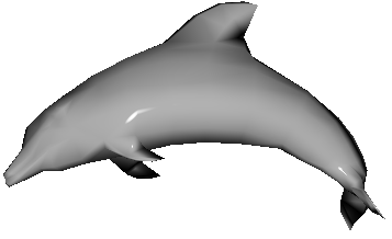
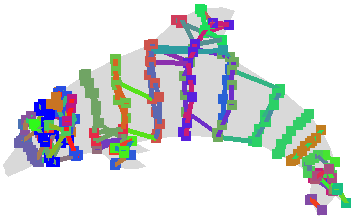
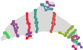
As the algorithms for the first two phases play an intrinsic role in our algorithm, we give a brief description of these.

Computing local separators is done through a two-step process. First a region growing approach is used to find a local separator. A vertex is picked, and we iteratively add to the separator an adjacent vertex and check if the neighbourhood is disconnected. We refer to this as growing a separator. Once a local separator has been found, it is heuristically minimised by removing vertices that would not destroy the separator. We refer to this as shrinking a separator.

Because the running time of LSS is often dominated by the search for local separators, a sampling scheme is used to reduce computation. According to the scheme, vertices are selected for separator computation with probability $2^{-x}$, where $x$ is the number of previously computed separators that contain that vertex.

Unfortunately, sampling only addresses the number of separators that need to be computed and not the time it takes to compute each separator. In this paper we address the latter issue using a multilevel approach. Specifically, we find separators on coarser versions of the graph and project them back up onto the original graph. Importantly, this allows us to set a patience threshold for the amount of computation that should be used to find a separator from a given vertex. When the threshold is exceeded we stop the search relying on a separator containing the given vertex to be found on a coarser level.

1.3 Related Work

Skeletonization, in terms of computing curve skeletons, is a diverse field not only in terms of interpretations of skeletons, but also in the algorithmic approaches. Several classifications of algorithms exist [11, 27], based on underlying traits of the algorithms.

The interpretation that the curve skeleton should lie on the medial surface, gives rise to methods that, in a sense, extract a curve skeleton from the medial surface of the input [12, 29, 19, 25, 32]. Since the medial surface is highly sensitive to noise, so are the skeletons generated by these methods.

A class of algorithms that are resilient to noise are the contractive methods, based on the concept of reducing the volume and surface area of the input until a skeleton is found [31, 4, 26]. In their simplest forms these algorithms require that the input be manifold, however it is possible to extend to other types of input [10, 17].

A related notion for shape analysis is that of Reeb graphs [7, 6]. These can be used for skeletonization, lending themselves to a topologically driven class of algorithms [22, 23, 13]. The resulting skeletons depend on a parameter, giving some flexibility in targeting specific properties of the output, but also requiring great care in the choice of the parameter.

In addition there are algorithms that fit into classifications not presented here [20, 14, 2].

A very successful heuristic approach to the NP-complete problem of graph partitioning is that of multilevel algorithms [9]. Although the problem considered is different, we employ a similar multilevel scheme for vastly improving practical performance. Such multilevel schemes have been extensively studied [15, 21, 1].

2 The Multilevel Framework

In its most general sense, the multilevel framework is a heuristic approach that aims to solve a problem by obtaining a solution to a smaller problem.

Initially, a series of increasingly simplified approximations of the input is generated. We call this the coarsening phase, and the series of simplifications we call levels. Since the last level is small, computing a solution is much faster. In graph partitioning literature, this is called the partitioning phase; however, we will consider it in terms of solving a restricted problem. Then, the solution found on the last level is transformed into a solution on the input through uncoarsening. This process is also sometimes called projection and refinement, since uncoarsening from one level to the previous is often done by projecting onto the previous level, and then employing some refinement process to improve the solution according to some heuristic.

By design, the multilevel framework is highly flexible. Various coarsening schemes can be used, that may prioritise preserving different properties of the input when simplifying. The restricted problem can be solved by any reasonable approach, and the refinement strategies can be adapted to suit the application.

Our algorithm works by first coarsening the input into several levels of decreasing resolution. The details of this coarsening is described in Section 2.1. Once the hierarchy of graphs has been generated, we do a restricted search for local separators on each level of resolution. The details are covered in Section 2.2, but the intuition is that searching for large local separators is slow in practice, and by restricting our search we save computation. Since the separators found are small, this does however also mean that we are only able to capture small features of the structure.

Figure 3: Visualisation of the multilevel skeletonization approach. A solid cylinder with a handle is coarsened until it is of small size. A number of small local separators are found (shown in blue), and then projected back to the original input. Searching for small local separators again yields the separators around the handle (shown in red), but separators are too large at this level to be discovered around the cylinder. We combine the separators to obtain a general solution.

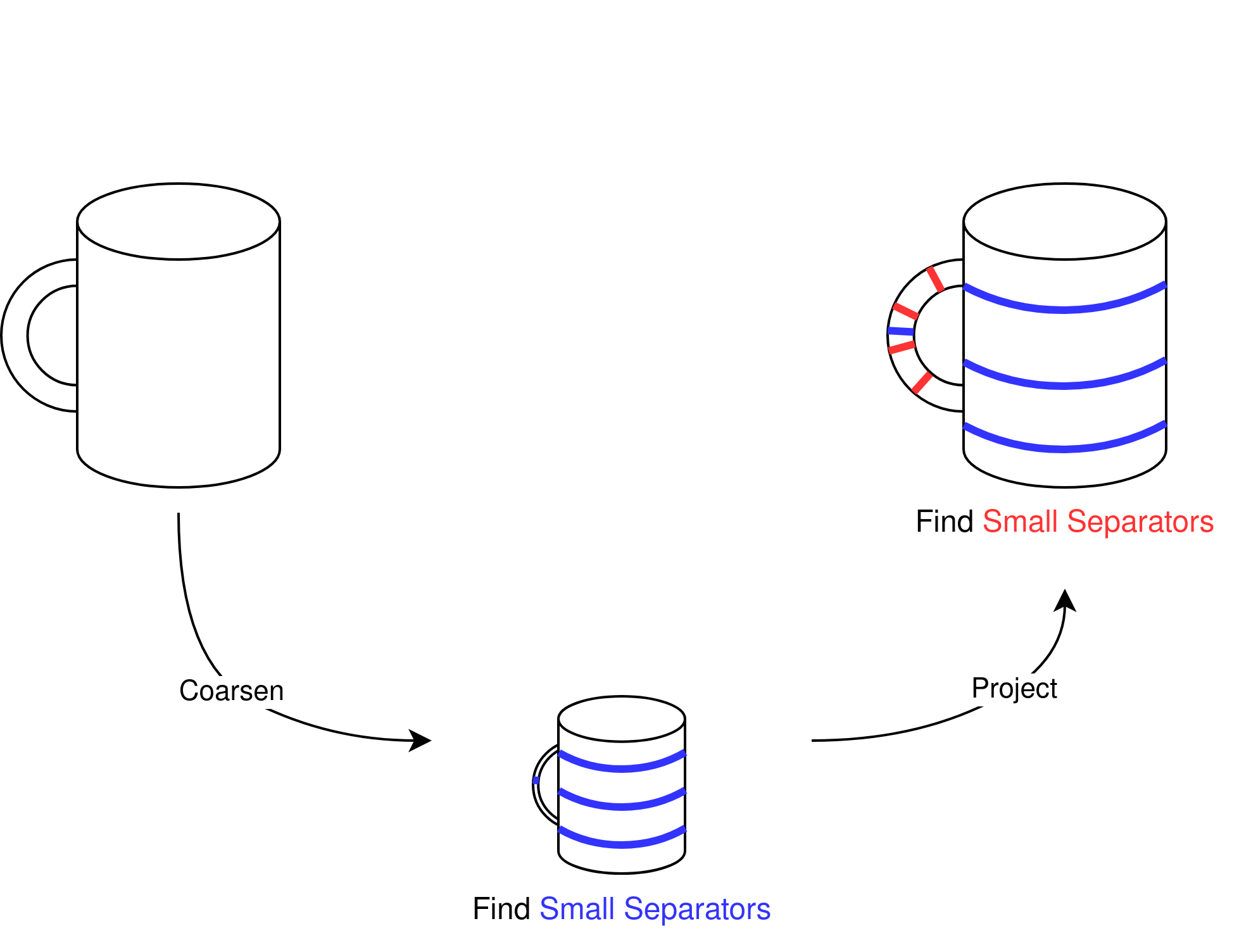
Since small features obtained on low resolution can represent large features on the original input, we obtain separators capturing features of varying sizes by searching for separators across every level.

By projection and refinement, see Section 2.3, we then transform the minimal local separators found across the levels into minimal local separators on the input. These can then be packed and extracted by the approach of LSS. The procedure is visualised in Figure 3.

2.1 Coarsening

Given as input a graph, $G=(V,E)$, we construct a sequence of increasingly simplified graphs, $G_{0},G_{1},\ldots,G_{l}$ s.t. $G_{0}\succ G_{1}\succ\ldots\succ G_{l}$ where $l=O(\log n)$ and $G_{i}\succ G_{j}$ denotes that $G_{j}$ is a minor of $G_{i}$, and $G_{i}=(V_{i},E_{i})$. Moreover $G_{0}=G$ and $\forall i\in[0,l),|V_{i}|\geq 2|V_{i+1}|$.

We do this by a matching contraction scheme, in which we repeatedly construct and contract maximal matchings. Various approaches to such coarsening schemes exist in literature [21], and from these, we choose to consider light edge matching.

To construct $G_{i+1}$ from $G_{i}$, greedily find a maximal matching and contract it. Such a matching can be constructed in $O(|E_{i}|)$ time by visiting vertices in a random order, matching them to an unmatched neighbour of smallest euclidean distance. We repeat this procedure until the number of vertices has been at least halved.

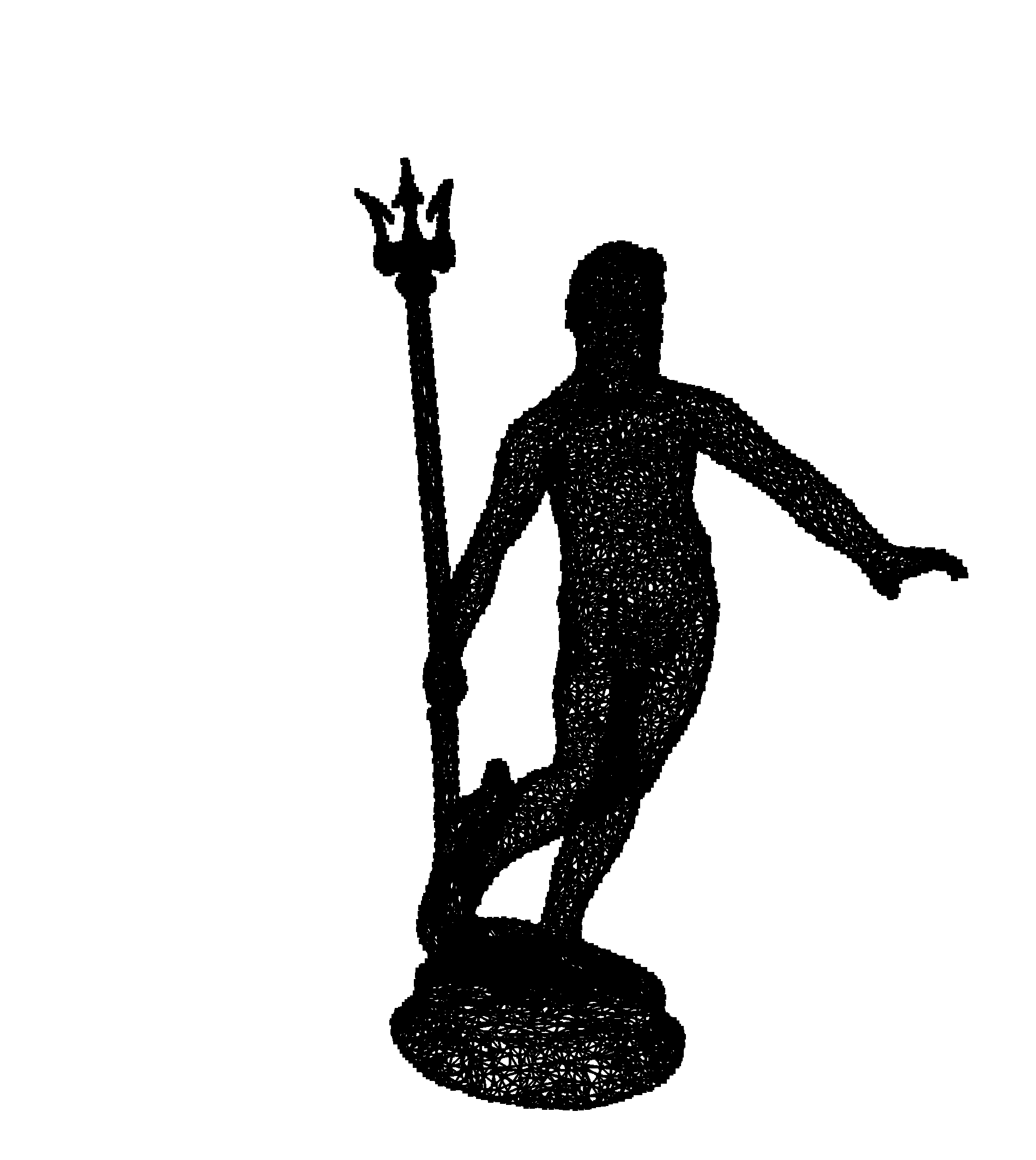
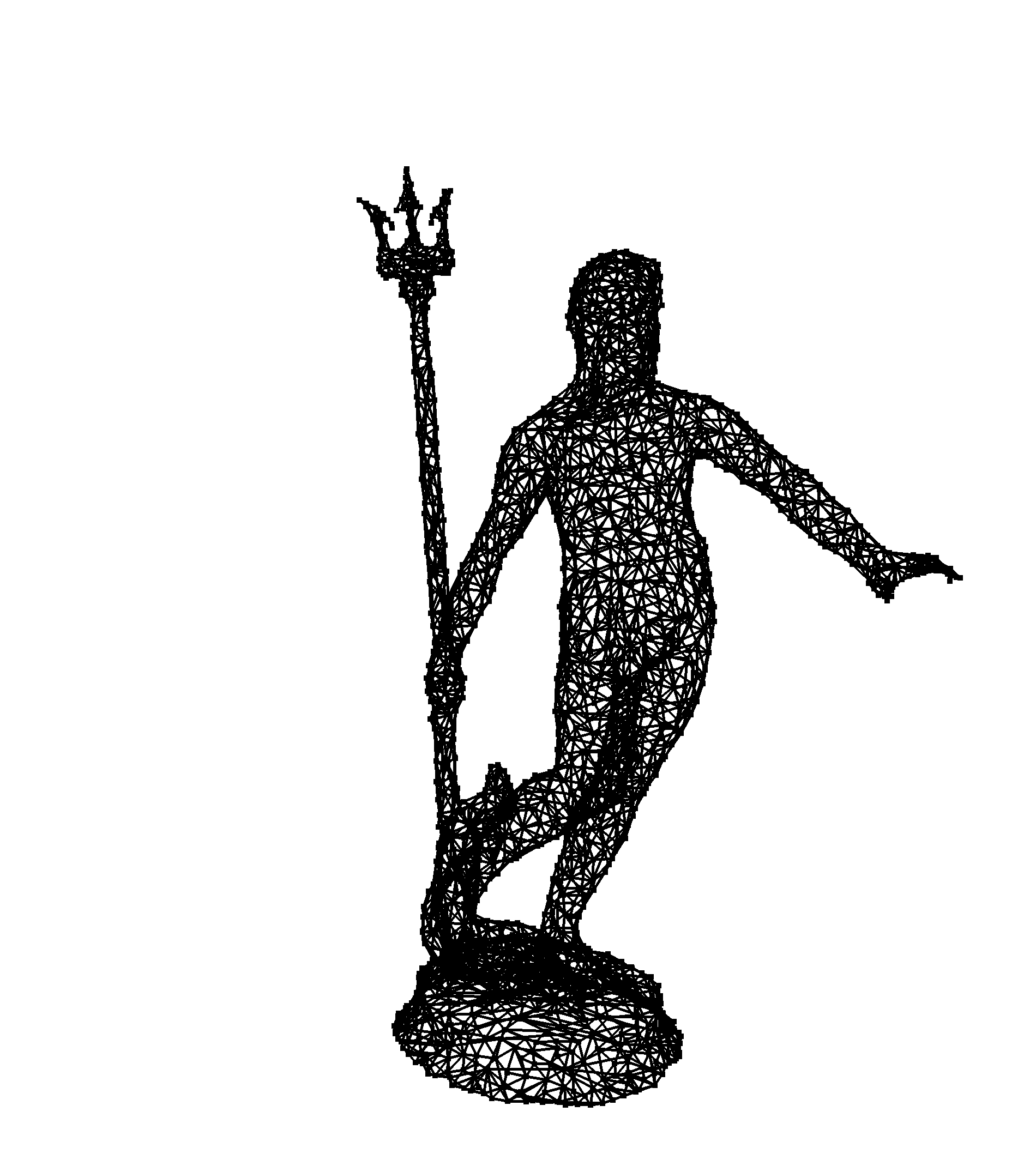
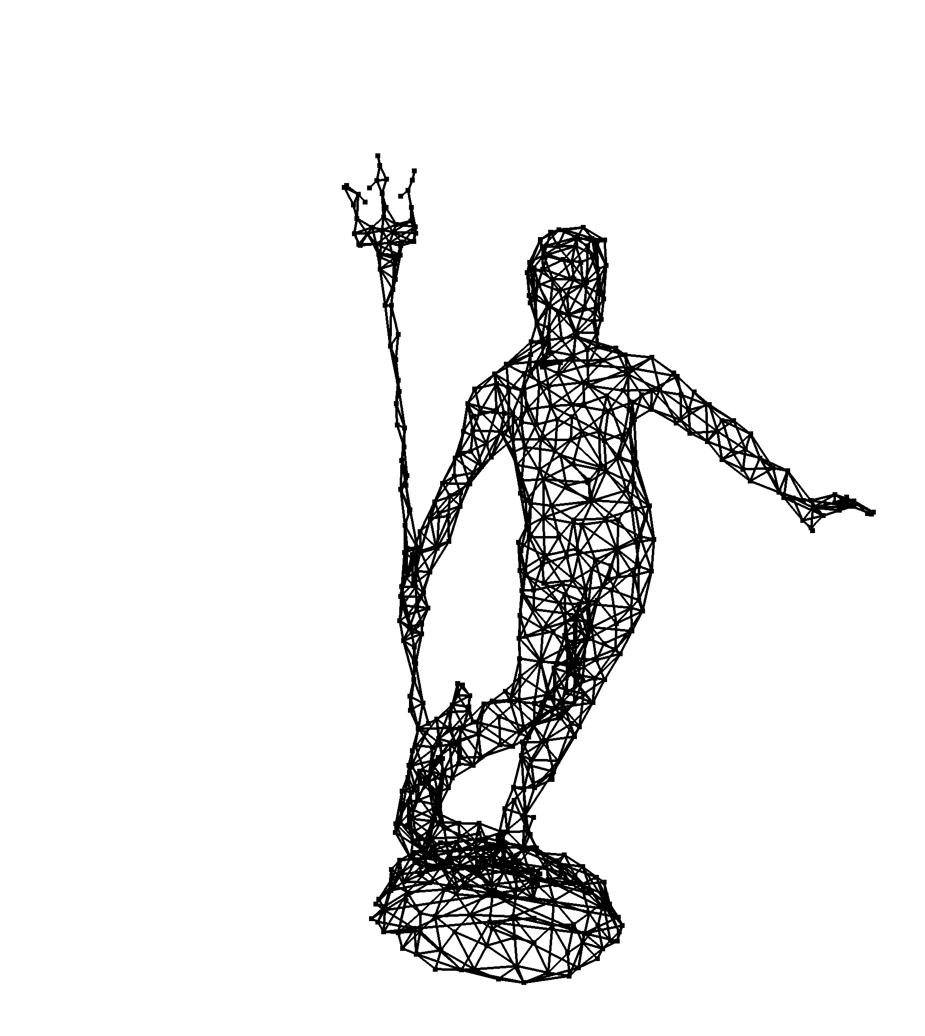
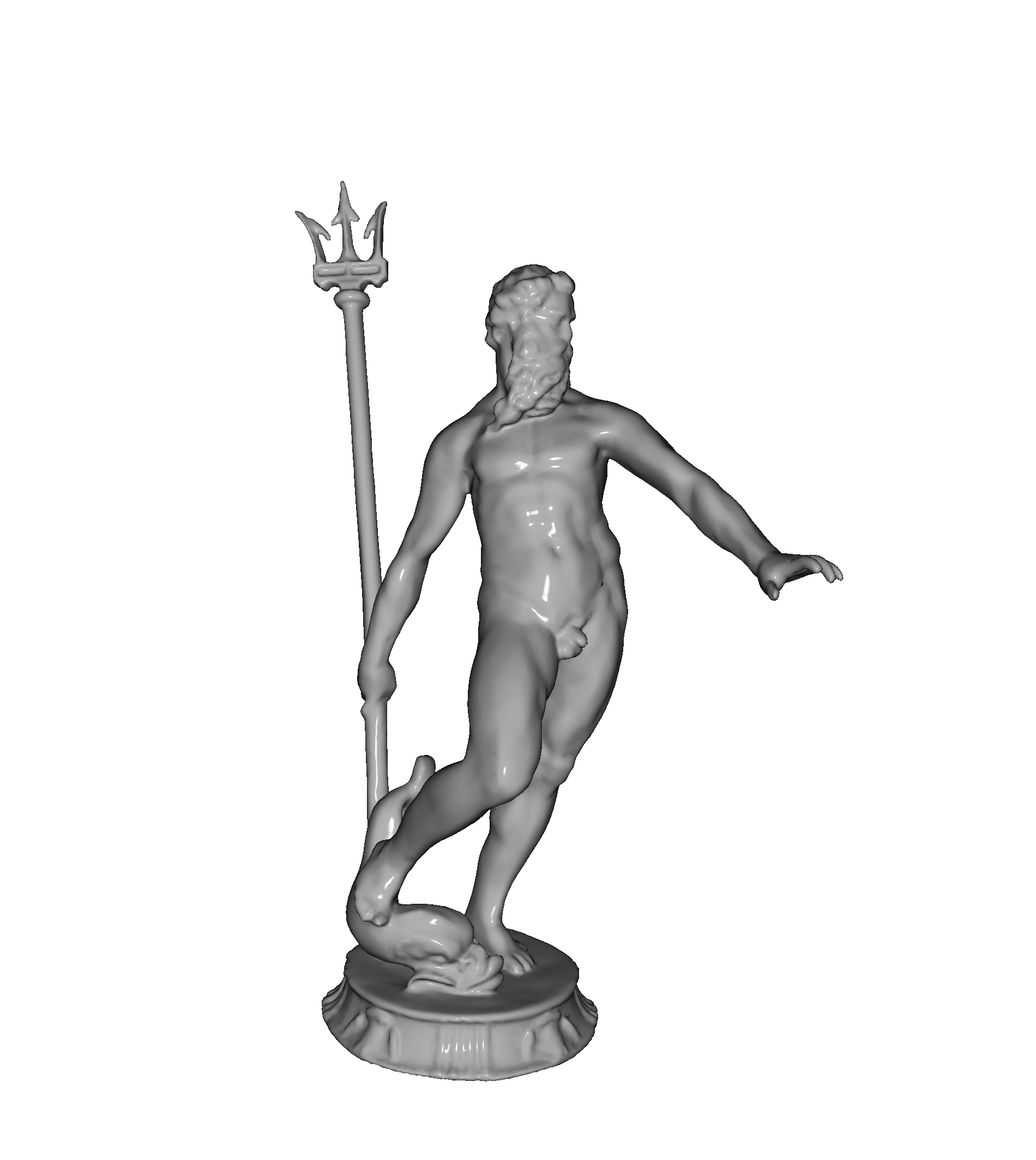
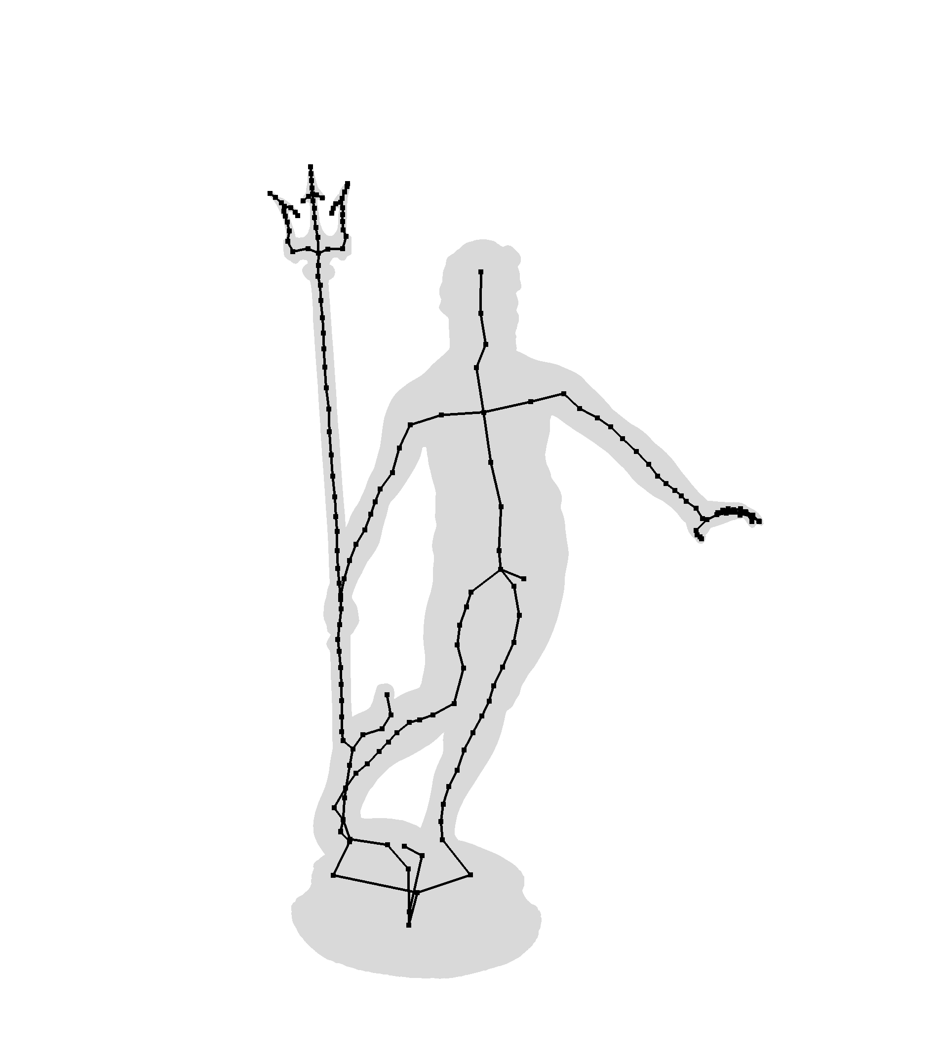
In Figure 4 we show some of the graphs obtained during coarsening of a triangle mesh resembling a statue of Neptune.

Figure 4: A series of increasingly simplified approximations of neptune.ply, from the Groningen Skeletonization Benchmark, obtained through light edge matching contraction.

Note that by contraction we always preserve the number of connected components. This is one of the homotopy-preserving properties of the algorithm.

Theoretical Analysis

In the worst case, we may spend $O(|V_{i}|)$ rounds of contraction in order to reach the desired number of vertices. This is a well known problem of matching contraction schemes on general graphs, but graphs obtained from the world of geometry tend to take a small number of rounds to contract [1].

A general bound on the time spent on the coarsening phase is then $\sum_{i=0}^{l}(|V_{i}||E_{i}|)=|E|\sum_{i=0}^{l}|V_{i}|=O(|V||E|)$. For graphs that are contracted in a constant number of rounds we get $\sum_{i=0}^{l}|E_{i}|$ and if we furthermore have $|E_{i}|=O(|V_{i}|)$, as is the case for triangle meshes and voxel grids, the bound becomes $O(|V|)$.

2.2 Restricted Separator Search

For a given connected set of vertices, $V^{\prime}$, we refer to the subgraph induced by vertices adjacent to $V^{\prime}$, that are not in $V^{\prime}$ themselves, as the front of $V^{\prime}$ and denote it $F(V^{\prime})$.

A region growing based approach to computing local separators is given in [5], where a separator, $\Sigma$, is iteratively grown until $F(\Sigma)$ is disconnected. The approach uses an enclosing ball around the vertices of $\Sigma$ to guide what vertex of $F(\Sigma)$ is added next, and the connectivity of $F(\Sigma)$ is then checked by traversal. As noted by the authors, it is possible to improve performance of the search by using a dynamic connectivity data structure to maintain the front, so that a traversal in every iteration is avoided.

In addition to adapting the algorithm to use a dynamic connectivity data structure, we will also restrict the number of iterations the search performs. Given a vertex, $v$, set $\Sigma_{0}=\emptyset,F_{0}=\{v\}$, and then iteratively construct $\Sigma_{i}=\Sigma_{i-1}\cup\{v_{i}\in F(\Sigma_{i-1})\}$, where $v_{i}$ is the closest neighbour of the front to an enclosing sphere around $\Sigma_{i-1}$. Maintain $F(\Sigma_{i})$, update the enclosing sphere and repeat until $F(\Sigma_{i})$ is disconnected or empty, or $|\Sigma_{i}|$ exceeds a threshold value. Pseudocode for this restricted separator search is shown in Algorithm 1.

Restricted-Separator-Search($G,v_{0},\alpha$):

      $\Sigma=\emptyset$

      $F=(\{v_{0}\},\emptyset)$

      $\mathbf{c}=\mathbf{p}_{v_{0}}$

      $i=0$

      $r=0$

      repeat

           $v=\arg\min_{f\in V(F)}\lVert\mathbf{c}-\mathbf{p}_{f}\rVert$

            // Scan front for closest vertex

           if $\lVert\mathbf{c}-\mathbf{p}_{v}\rVert>r$ then

                $r=\frac{1}{2}(r+\lVert\mathbf{c}-\mathbf{p}_{v}\rVert)$

                 // Update the sphere

                $\mathbf{c}=\mathbf{p}_{v}+\frac{r}{\epsilon+\lVert\mathbf{c}-\mathbf{p}_{v}\rVert}(\mathbf{c}-\mathbf{p}_{v})$

               

                $\Sigma=\Sigma\cup\{v\}$

                remove($F,v$)

                for $(x,y)\in E(\textnormal{{Neighbourhood(}}\textnormal{\emph{G,v}}\textnormal{{)}}-\Sigma)$ do

                     connect($F,x,y$)

                      // Maintain the front of $\Sigma$

                    

                     $i=i+1$

                    

                     until number-of-components($F$)$>1$ or $i=\alpha$

                    if $\textnormal{{number-of-components(}}\textnormal{\emph{$F$}}\textnormal{{)}}=1$ then

                         return $\emptyset$

                          return $\Sigma$

Given a spatially embedded graph, $G$, a starting vertex, $v_{0}$, and a thresholding value, $\alpha$, search for a separator of size at most $\alpha$ and return it, or $\emptyset$ if failure. Here $\epsilon$ is a small constant to prevent division by zero.

Algorithm 1 Restricted Separator Search

Given a spatially embedded graph, $G$, a starting vertex, $v_{0}$, and a thresholding value, $\alpha$, search for a separator of size at most $\alpha$ and return it, or $\emptyset$ if failure. Here $\epsilon$ is a small constant to prevent division by zero.

Theoretical Analysis

We analyse the complexity of this restricted separator search in terms of the graph $G^{\prime}=\Sigma\cup F(\Sigma)$ with $n^{\prime}$ vertices and $m^{\prime}$ edges, using the dynamic connectivity data structure of Holm, de Lichtenberg and Thorup with updates in amortized $O(\log^{2}n^{\prime})$ time [16]. Since the size of the separator is at most $\alpha$ and we add one vertex each iteration, we use at most $\alpha$ iterations selecting the closest vertex from the front, updating the bounding sphere and maintaining the dynamic connectivity structure. Selecting the closest vertex is done naively with a scan through the front, taking $O(n^{\prime})$ time and updating the bounding sphere takes $O(1)$ time each iteration. This gives a running time of $O(\alpha n^{\prime})$. Each edge in the dynamic connectivity structure is inserted and removed at most once, with each operation taking $O(\log^{2}n^{\prime})$ amortized time, totalling $O(m^{\prime}\log^{2}n^{\prime})$. The total running time is then $O(\alpha n^{\prime}+m^{\prime}\log^{2}n^{\prime})$.

In the general case we give no better worst case bound than $O(\alpha|V|+|E|\log^{2}|V|)$. For graphs of bounded maximum degree we can bound the size of the front. Let $\Delta$ be the maximum degree of $G$, then $n^{\prime}=O(|\Sigma|\Delta)=O(\alpha\Delta)$ and $m^{\prime}=O(\alpha\Delta^{2})$. This gives a time of $O(\alpha^{2}\Delta+\alpha\Delta^{2}\log^{2}(\alpha\Delta))$. In addition if we choose $\alpha$ to be a small constant, the bound is further improved to $O(\Delta^{2}\log^{2}\Delta)$. For graphs where $\Delta=O(1)$ as for voxel grids or knn-graphs, the search then becomes $O(1)$. Note that for this bound to be applicable across the entirety of the algorithm, the degree needs to remain bounded through coarsening.

2.3 Projection and Refinement

For projecting separators to graphs of higher levels of detail, we employ a simple uncoarsening technique. By storing information about what vertices were contracted during coarsening, we can reverse the contractions that gave rise to the vertices of a given separator. Note however that a separator that has been projected in such a way is not guaranteed to be minimal.

The simplest refinement scheme is thus one that uses the algorithm for minimising separators as in LSS. The minimising algorithm is a heuristic approach that seeks to minimise a separator such that the structure becomes that of a thin band. When used on separators that are obtained through projection, there is not necessarily much room for choice. Therefore we consider a variation of our refinement scheme, we thus choose to "thicken" the separators after projection, by adding the adjacent vertices if it would not destroy the separator. This gives the heuristic minimisation more options for creating separators of shorter length, as visualised in Figure 5.

Figure 5: A separator undergoing expansion as part of refinement. (A) shows an input, (B) a coarsened representation, (C) a computed separator denoted by red vertices, (D) the projected separator denoted by red vertices and the added vertices denoted by orange, (E) shows the separator obtained by minimising the thickened separator.

Projecting a separator can be done in linear time proportional to the size of the resulting separator, while the minimisation in worst case takes quadratic time (see Appendix C.2).

After processing each separator in this way, we obtain a set of minimal separators for the current level. If we accumulate separators indiscriminately, we will spend time projecting and refining separators that will ultimately be discarded due to overlapping. If we perform set packing on every level, we are going to be too eager in our efforts, discarding things that might not overlap once projected further. Intuitively, we would like to only discard separators if there is a large overlap.

To do this, we associate with each vertex, $v$, of every graph, $G_{i}$, a capacity, $c_{v}^{i}$, equal to the sum of capacities of vertices contracted to obtain it. For vertices of $G_{0}$ we define the capacities as $1$, formally $\forall v\in V(G_{0}),c_{v}^{0}=1$. In this way, the capacity of a given vertex is the number of vertices of the original input that it represents.

We then modify the greedy set packing algorithm of LSS, so that we include a separator iff it would not cause any vertex to exceed its capacity. Since the capacities of $G_{0}$ are $1$, this packing is equivalent to the original when applied to the highest level of resolution, and thus we will still have a non-overlapping set of separators at the end.

Note however that this packing allows for duplicates to persist through packing, essentially reducing the capacities of vertices while providing no valuable information. To counteract this, we perform a filtering step using hashing to rid duplicates prior to the packing procedure. Filtering and packing in this way takes time linear in the sum of sizes of separators in the set.

2.4 The Multilevel Skeletonization Algorithm

With the details of the phases in place, we can then combine these to construct the multilevel skeletonization algorithm. Given a spatially embedded input graph, $G=(V,E)$, and a threshold value $\alpha$, we construct a curve skeleton by the following:

Generate $G_{i}$ from $G_{i-1}$ by coarsening, until $|G_{l}|\leq\alpha$ for some $l$. This generates the sequence of graphs of decreasing resolution $G_{0},G_{1},\ldots,G_{l}$ where $l=O(\log|V|)$ and $\sum_{i=0}^{l}|V_{i}|=O(|V|)$.

Then, starting at the lowest resolution, $G_{l}$, find restricted separators. We do this by the restricted separator search, starting at each vertex with probability $2^{-x}$, where $x$ is the number of currently computed separators containing that vertex, using $\alpha$ as the restriction on the size of the search. After computing the separators for a level, we perform capacity packing, and then we project the computed separators to the next level and refine them. This process is repeated for every level until we arrive at the original graph. At this point, after performing capacity packing, we obtain a non-overlapping set of minimal separators from which we extract the skeleton, using the extraction procedure of LSS [5]. Pseudocode for this algorithm can be seen in Algorithm 2.

Multilevel-Skeletonization($G,\alpha$):

      $G_{0}=G$

      $l=0$

      repeat // Coarsening phase

           $l=l+1$

           $G_{l}=\textnormal{{Coarsen(}}\textnormal{\emph{$G_{l-1}$}}\textnormal{{)}}$

          

           until $|V(G_{l})|\leq\alpha$

          $S=\emptyset$

            // Maintain set of minimal separators

           for $i=l$ to $0$ do // From low to high resolution

                $S^{\prime}=\emptyset$

                for $s\in S$ do // Project and refine from previous levels

                     $S^{\prime}=S^{\prime}\cup\textnormal{{Project-Refine(}}\textnormal{\emph{$s$}}\textnormal{{)}}$

                    

                     $S=S^{\prime}$

                     for $v\in V(G_{i})$ with probability $2^{-x(v)}$ do // Search on this level

                          $s=\textnormal{{Restricted-Separator-Search(}}\textnormal{\emph{$G_{i},v,\alpha$}}\textnormal{{)}}$

                          $S=S\cup\{\textnormal{{Minimise-Separator(}}\textnormal{\emph{s}}\textnormal{{)}}\}$

                         

                          $S=\textnormal{{Capacity-Pack(}}\textnormal{\emph{$S$}}\textnormal{{)}}$

                         

                          return Extract-Skeleton($G,S$)

Given a spatially embedded graph, $G$, and a thresholding value, $\alpha$, compute a curve skeleton.

Algorithm 2 Multilevel Skeletonization

Given a spatially embedded graph, $G$, and a thresholding value, $\alpha$, compute a curve skeleton.

Theoretical Analysis

For completeness’ sake we consider then the complexity of the algorithm. Recall that the coarsening phase in the general worst case takes $O(|V||E|)$ time, but for not too irregular input takes $O(|V|)$ time. We then perform a restricted separator search from each vertex across every level, which is $O(\alpha|V|^{2}+|V||E|\log^{2}|V|)$ in the general worst case, but $O(\alpha|V|)$ for graphs that retain constant bounded degree through coarsening. We consider then the time a single separator contributes to the total when expanding, filtering and packing. These operations are linear in the size of the separator on each level, which is worst case $O(|V_{i}|)$ on level $i$. This totals $\sum_{i=0}^{l}O(|V_{i}|)=O(|V|)$ for a single separator across all levels. Minimizing a single separator takes worst case $O(|V_{i}|^{2})$ on level $i$, which for a single separator contributes $\sum_{i=0}^{l}O(|V_{i}|^{2})=O(|V|^{2})$ across all levels. We also perform packing on each level, linear in the sum of sizes of separators, which in total takes $\sum_{i=0}^{l}O(|V_{i}|^{2})=O(|V|^{2})$ time. The general worst case bound then becomes $O(|V|^{3}+|V||E|\log^{2}|V|)$, which is an improvement over LSS. It is worth mentioning however, that in practice the running time for both LSS and our algorithm is heavily dominated by the search for separators, and that theoretically expensive procedures, such as minimisation, make up only a small fraction of the running time.

3 Experiments

In this work, our main objective was to make an algorithm that produces the same quality of skeletons as LSS [5], only with improved running times, using new algorithmic ideas and algorithm engineering. As we will show in this section, the improvements to practical running times are very satisfactory.

As for quality, it is our overall assessment that the quality has not been compromised by the speed-up.

There is, however, no standard for how skeletons should be compared. In [27] it is remarked that quantifying the quality of skeletons is an open challenge, but we shall instead compare ourselves only to skeletons obtained by LSS, to quantify the deviation obtained by employing the multilevel approach.

To do this, we will measure a number of metrics, namely the number of vertices in the skeleton, the number of leaf nodes, branch nodes, chordless cycles which estimates the genus of the input, and the directed Hausdorff distance in both directions. For our comparisons, it is the relationship between directed Hausdorff distances that matter, rather than the magnitudes. A high distance from an LSS skeleton to our skeleton, with a low distance the other way, could indicate that LSS captures a feature that our skeleton does not. Likewise for the inverse, which might indicate that we are capturing a feature that LSS does not deem to exist. We give our Hausdorff distances divided by the radius of a bounding sphere, to reduce influence from the differing scales of input.

We run our tests on the Groningen Skeletonization Benchmark [28], consisting of several triangle meshes of varying structure. The test are executed on HPC Cluster nodes with Xeon Gold 6226R (2.90GHz) CPUs, using 8 cores of a single CPU for each test. For running time measurements, tests are run three times, and the median value is reported.

For comparisons we examine three algorithms, namely the local separator skeletonization algorithm (LSS) [5], our multilevel algorithm using light edge matchings, described in Section 2.1, as contraction scheme (LEM) as well as with light edge matchings and thickened separators, described in Section 2.3, as the refinement scheme (LEMTS).

We note that the variation of LSS with which we compare our algorithms also includes usage of a dynamic connectivity structure, so that the search procedures are identical up to the threshold parameter.

Implementation

Our implementation is written in C++, built into a fork of the GEL library, and made publicly available [18]. This is the same library that contains LSS, and as such our algorithms use the same underlying data structures and subroutines. All programs are compiled using -O3 optimisation flags. Details regarding the dynamic connectivity structure are given in Appendix C.1. We run the restricted searches in parallel internally on each level, using a simple fork-join pattern, identical to that of LSS. To account for the multilevel structure of our algorithm, we then pack using a single thread, project using at most two threads and repeat the pattern for the next level. The decision to use only two threads for projection stems from the fact that the overhead associated with spinning up threads quickly outweighs the benefits of parallel projection since there are often few separators after packing.

3.1 Results

Here we present our results in terms of measurements on the Groningen Skeletonization Benchmark. Initially we argue for our choice of $\alpha$, showing how the threshold impacts both skeleton quality as well as running time. We then present a number of results relating to the skeletons themselves to showcase the quality of output. We then present our measurements of running times, as well as discuss interesting observations.

Additional measurements are presented in Appendix A and Appendix B.

The Right Amount of Patience – Determining a Threshold Value $\alpha$

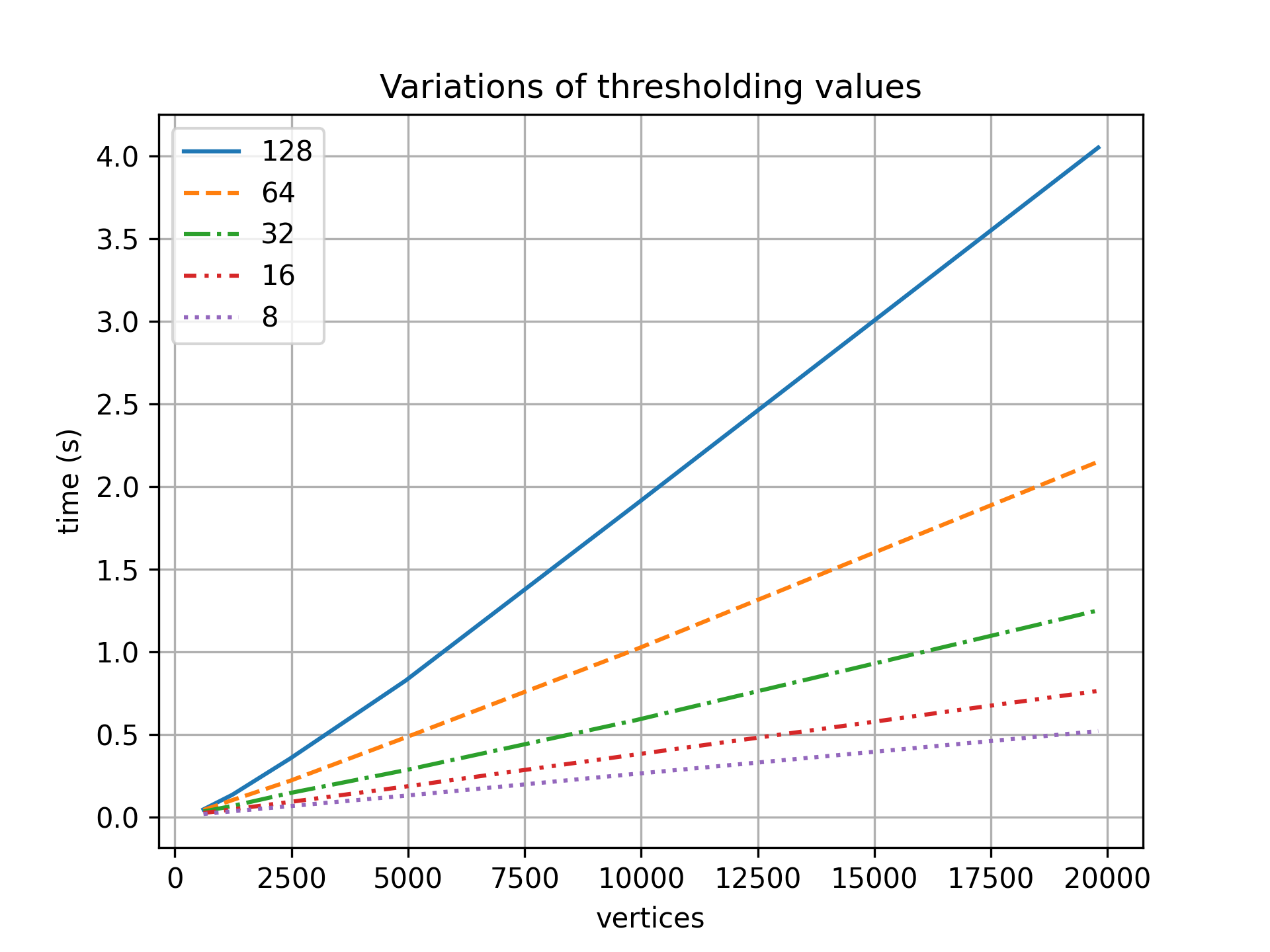
To show the effects of $\alpha$ on the running time, we consider a small test suite using subdivisions of a mesh to generate various sizes of input. This is done to ensure a similar underlying structure throughout the test. We test our multilevel algorithm for $\alpha=8,16,32,64,128$ (see Figure 6). Not surprisingly, a lower threshold leads to a lower running time.

Figure 6: Running time measurements of varying values of $\alpha$ on subdivisions of a mesh.

Figure 7: Skeletons found on human_hand.ply for increasing patience thresholds. From left to right: $\alpha=8,16,32,64,128$.

However, there may be a trade-off between skeleton quality and threshold value, which we explore qualitatively.

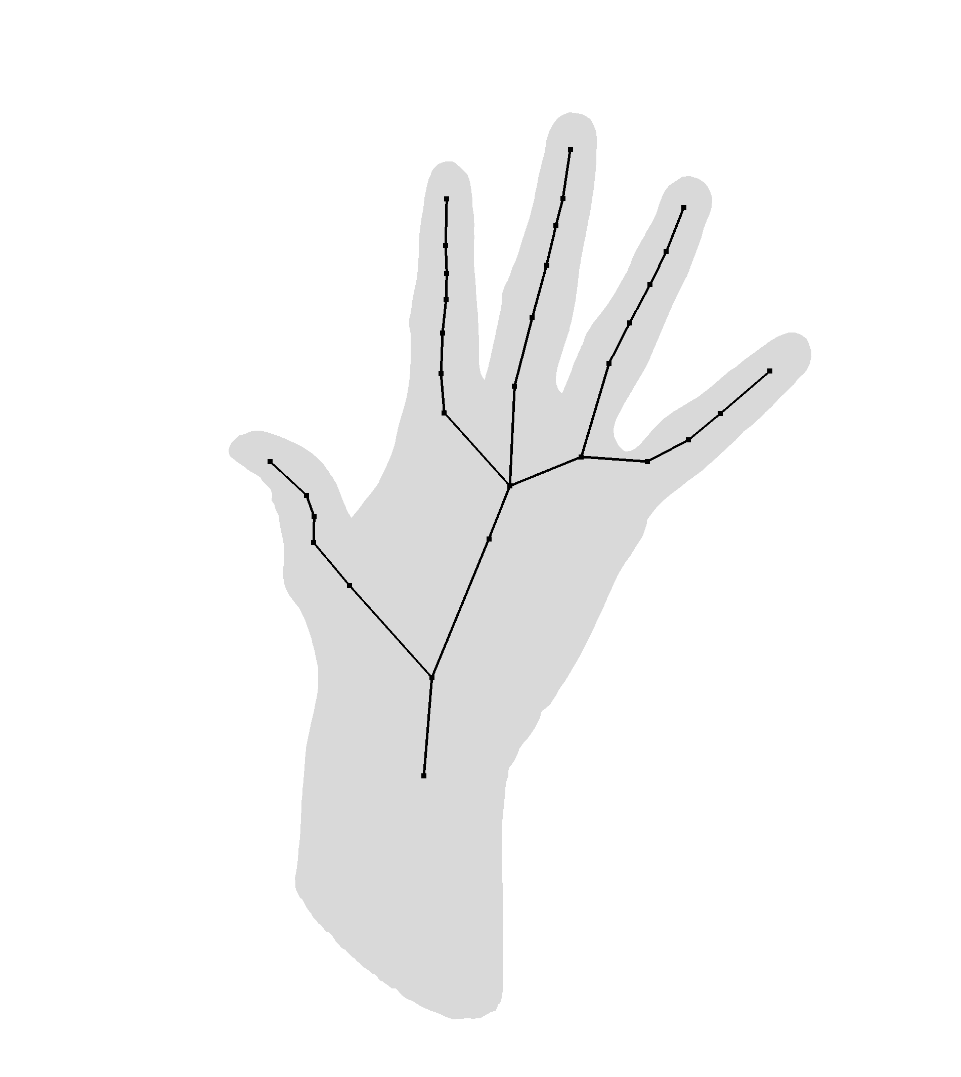
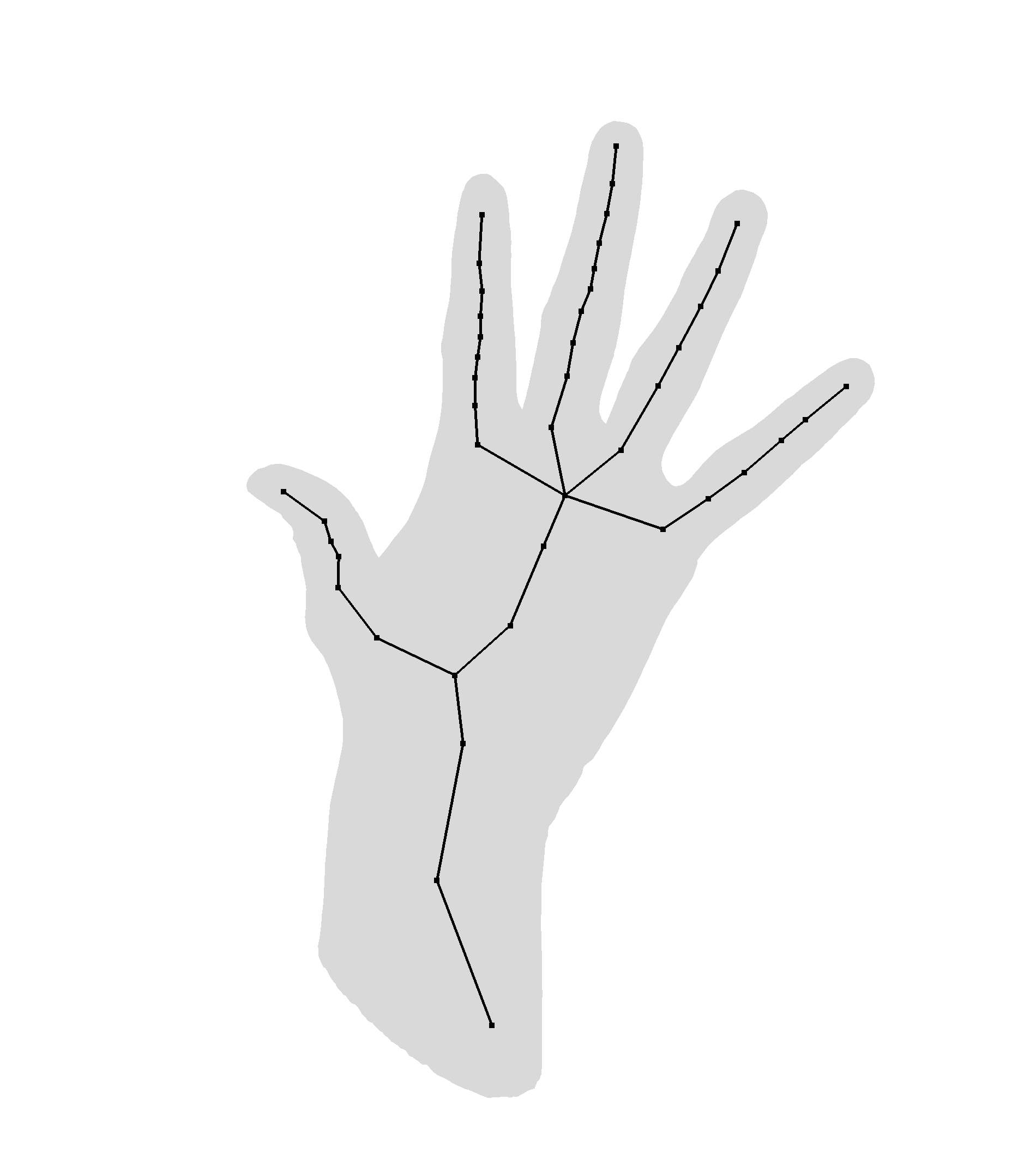
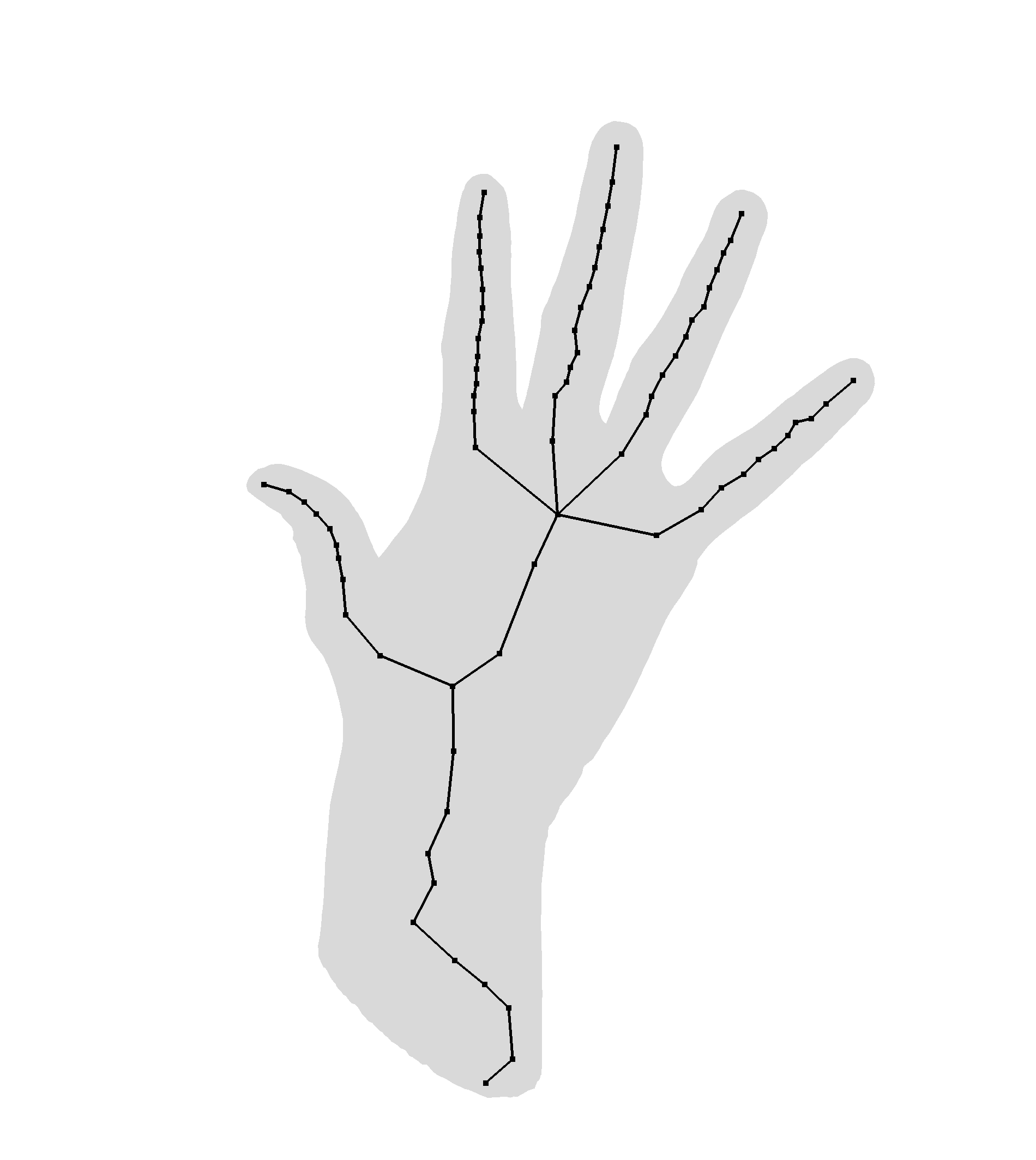
We visually examine the skeletons generated for our choices of $\alpha$ on human_hand.ply, as seen in Figure 7. For very low values of $\alpha$, the skeletons have few curves in areas that are relatively thick. With a low threshold, separators must be found on lower resolutions, which in turn means that few separators can be found. As we progress to higher values of $\alpha$, the level of detail of the skeleton rises, up to a certain point. Intuitively, if the threshold is high enough that the details can be captured on the higher levels of detail, then we gain nothing from the lower resolution levels.

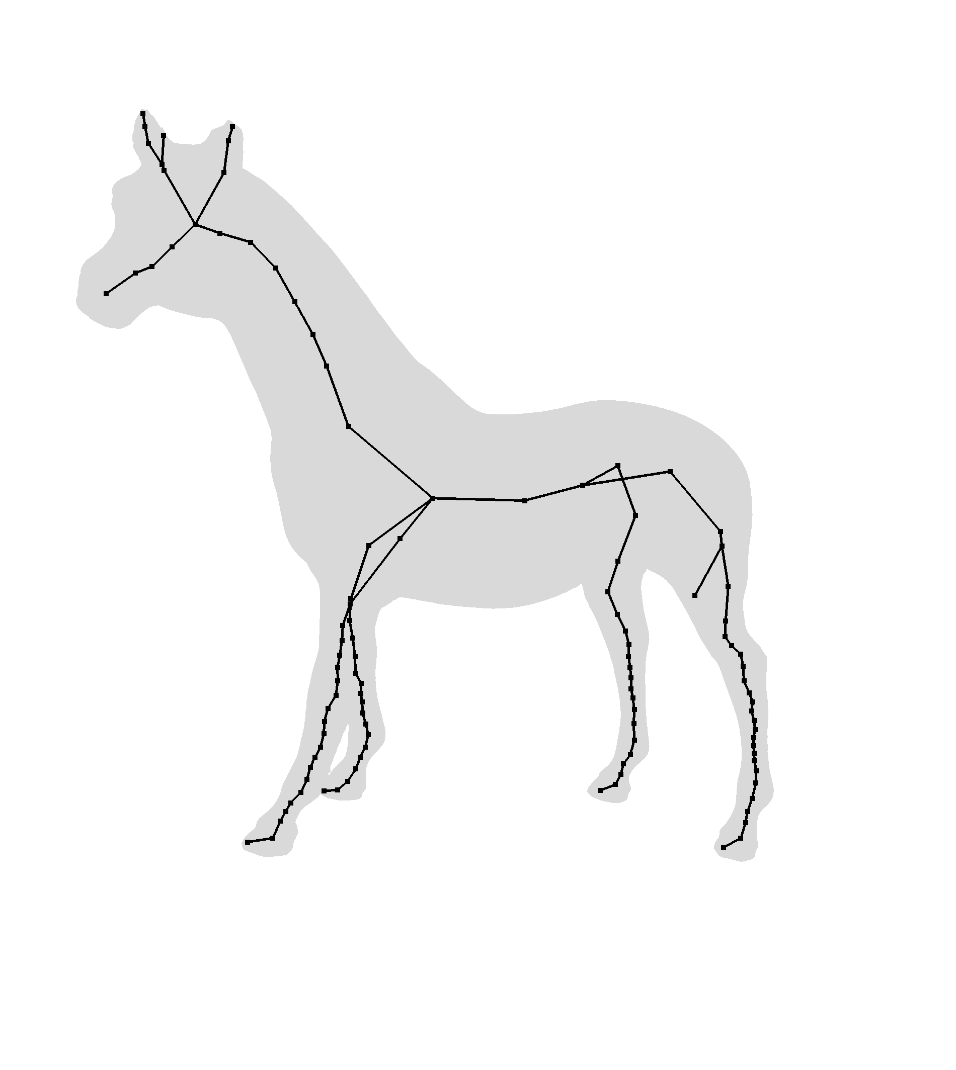
It could be argued that $\alpha=16$ or $\alpha=32$ generates the most visually appealing skeletons for this particular input, however we find that $\alpha=64$ offers the best trade-off for running time on other examined input such as that shown in Figure 8.

Thus, we run the remainder of our tests using $\alpha=64$.

Figure 8: Each column indicates a different input, with each row showcasing a different method. From top to bottom: shaded renders of the input, skeletons obtained by LSS, skeletons obtained by LEM, skeletons obtained by LEMTS

Skeleton Quality

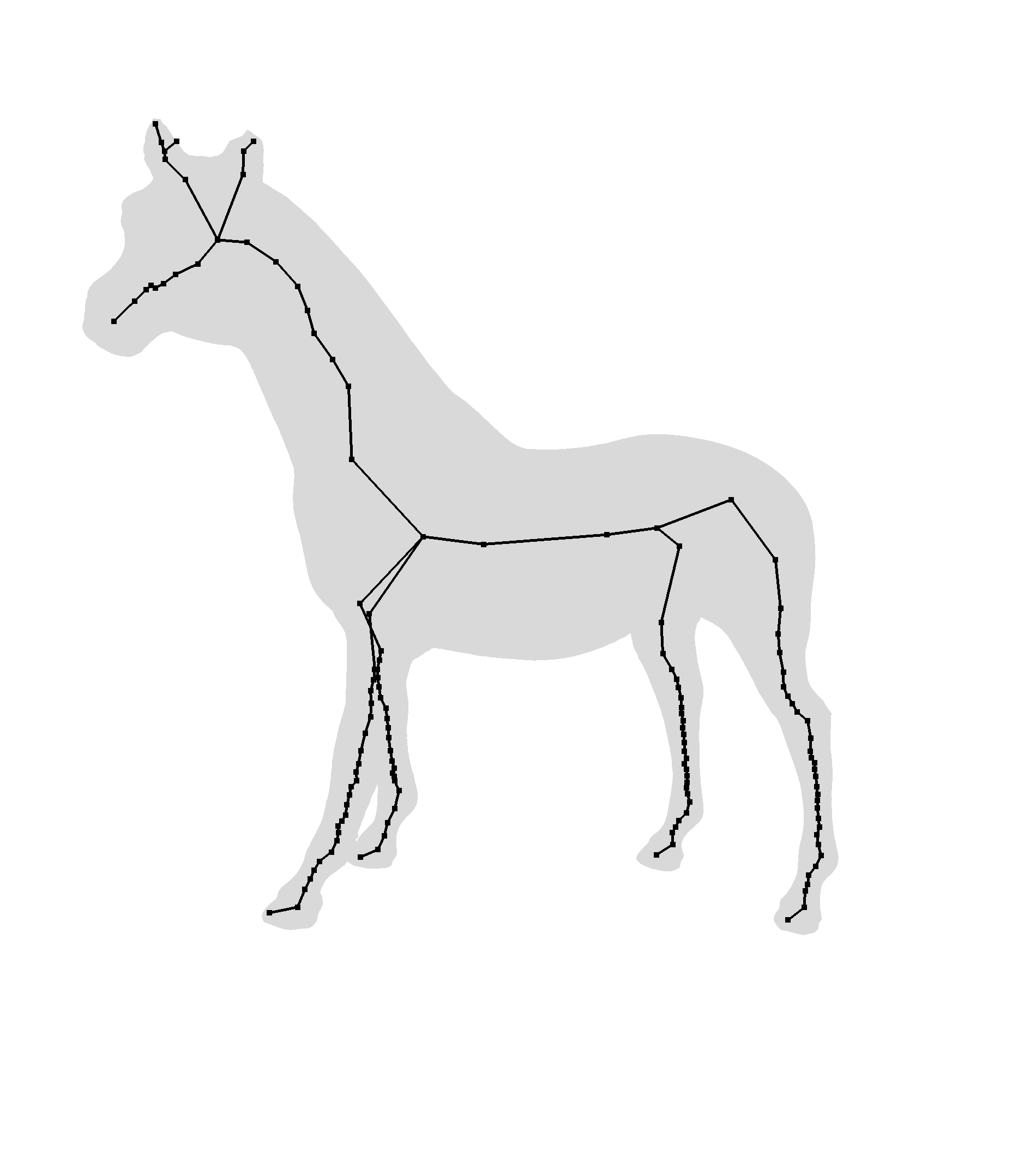
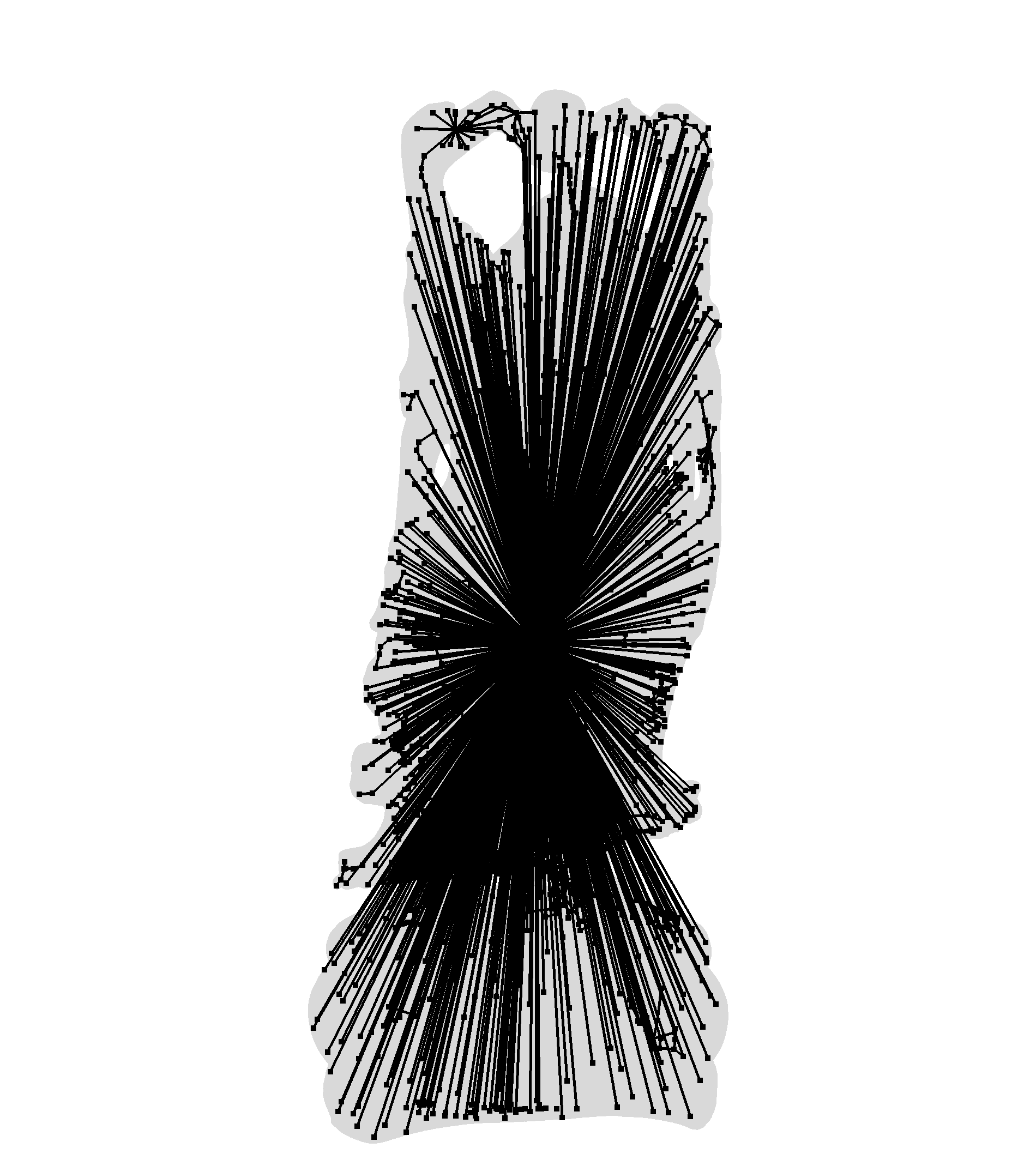
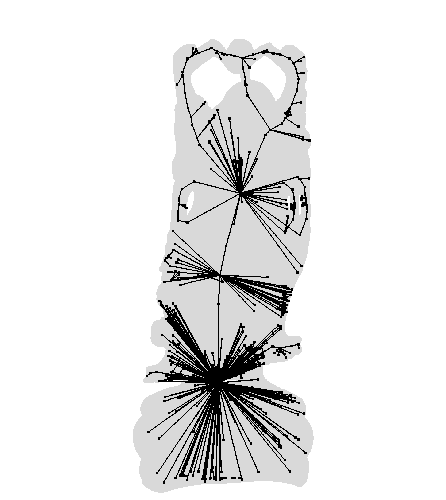
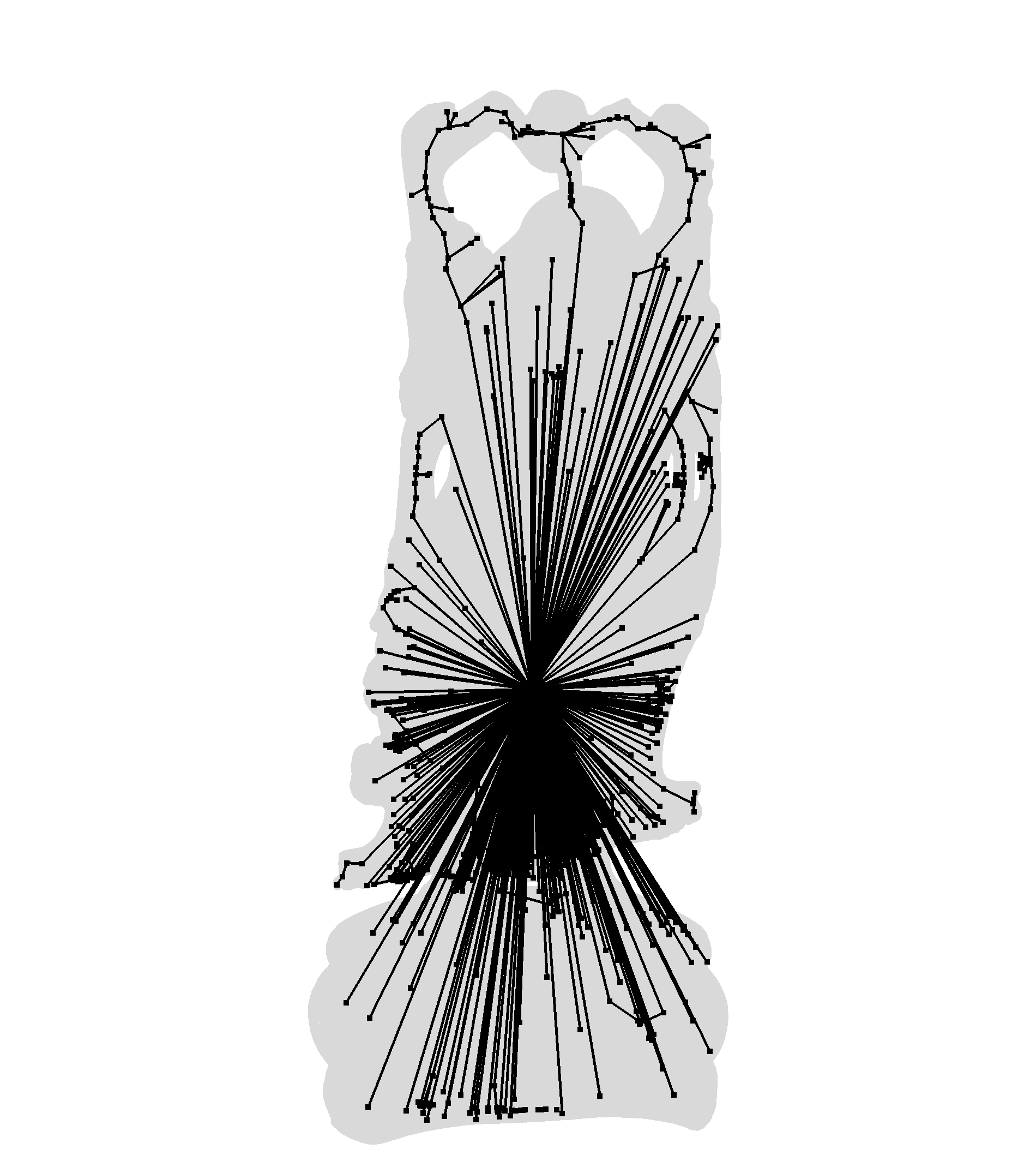
In Figure 8 we show some of the skeletons obtained by LSS, LEM and LEMTS. Note that both LEM and LEMTS appear smoother, while also reaching the features that LSS finds in many cases. In addition, it seems that for these inputs our methods find less spurious features, giving a cleaner result. When comparing LEM and LEMTS the differences are subtle. On horse.ply it can be seen that the vertex where the front legs meet the body is positioned further to the left. This is due to LEMTS having a denser skeleton. On the other hand, LEMTS seems to not capture the structure of the groin area of neptune.ply as well as LEM. Although it appears as if LEMTS finds a cycle, this is not actually the case. The skeletal branch is, however, not positioned as one would expect.

input	algorithm	$\Delta$vertices	$\Delta$leafs	$\Delta$branches	$\Delta$genus	$H(*,LSS)$	$H(LSS,*)$
19465	LEM	-563	-3	-35	2	0.0437028	0.0415616
	LEMTS	-416	11	-24	3	0.0355444	0.0382796
fertility	LEM	-46	-3	-1	0	0.273804	0.0874419
	LEMTS	-30	-3	-1	0	0.240033	0.165239
happy4	LEM	-589	-409	-21	-100	0.199295	0.0887277
	LEMTS	-560	-384	-22	-99	0.160472	0.100934
horse	LEM	-95	-1	-1	0	0.112222	0.111066
	LEMTS	-66	-2	-2	0	0.0883287	0.0851157
neptune	LEM	-73	-16	-5	0	0.200924	0.0508065
	LEMTS	-51	-15	-1	0	0.225756	0.0516766

Table 1: Excerpt of measurements on skeletons. The metrics denoted by $\Delta$ are relative to the skeletons of LSS, with negative values implying that LSS has more vertices, leafs, branches etc. Here $H(A,B)$ denotes the directed Hausdorff distance between $A$ and $B$, divided by the radius of a bounding sphere, and $*$ denotes skeletons generated by our multilevel algorithms.

In addition, we also showcase a small excerpt of measurements from Appendix B, which can be seen in Table 1. Here it is clear that LEM and LEMTS produce slightly simpler skeletons with fewer vertices, leaves, and branches. However, from visual inspection of the models it is clear that (at least for the models in the table) the missing details in the skeleton correspond to features which are so subtle that the skeletal details might be considered spurious. For all inputs of the benchmark except happy4.ply, there is little deviation in the genus compared to LSS.

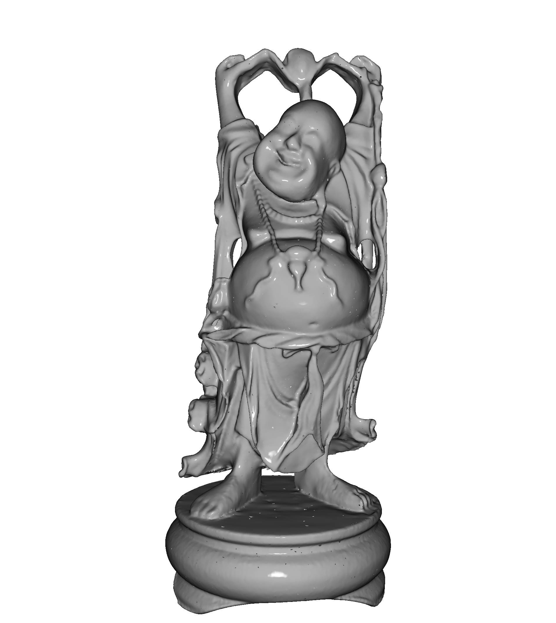
For context on the strange genus found on happy4.ply, we show the generated skeletons in Figure 9. Of note is that the mesh has several missing patches, which seems to cause spurious small separators to be found on all of the local separator based methods. We consider this an error case for all of the methods examined.

Figure 9: A triangle mesh with a large number of missing patches on the surface, happy4.ply, resulting in erroneous output for LSS, LEM, and LEMTS

Running Time

Although the running time of local separator skeletonization methods depends very much on the search for separators, which in turn depends on the structure of the input, we give the running times of the examined methods in Figure 10 as a function of the number of vertices in the input, over the entirety of the Groningen Skeletonization Benchmark [28].

(a) Running times of LSS.

(b) Running times of LEM.

Figure 10: Running times in total (top) and for searching (bottom) as function of the number of vertices on the Groningen Skeletonization Benchmark. Values over 20 hours omitted.

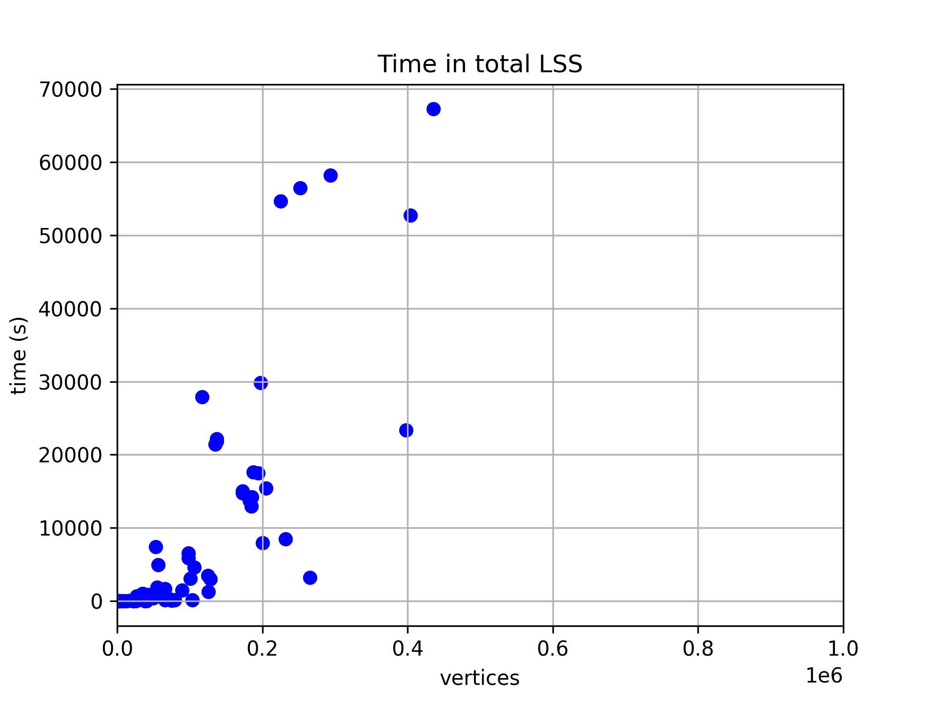
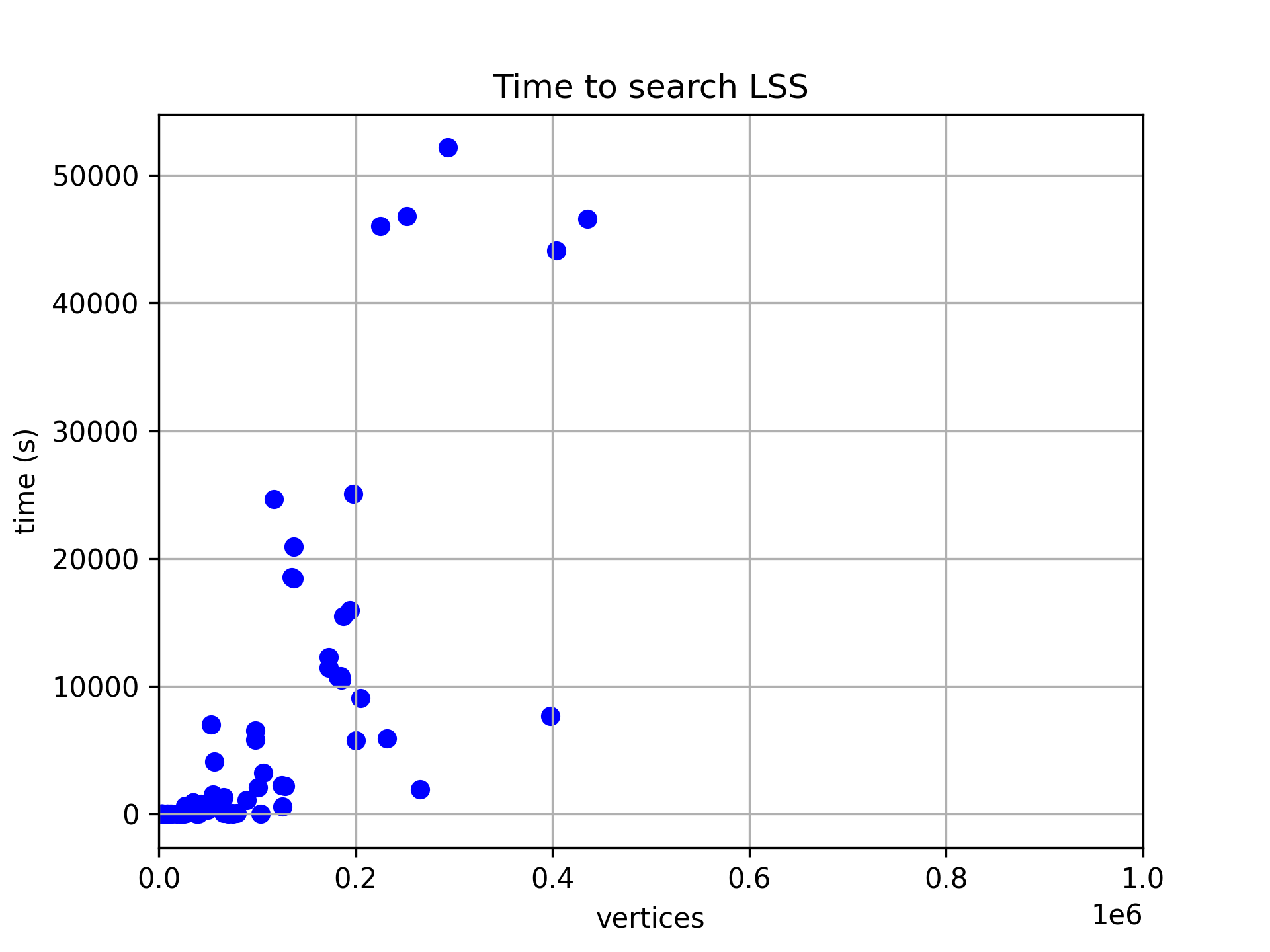
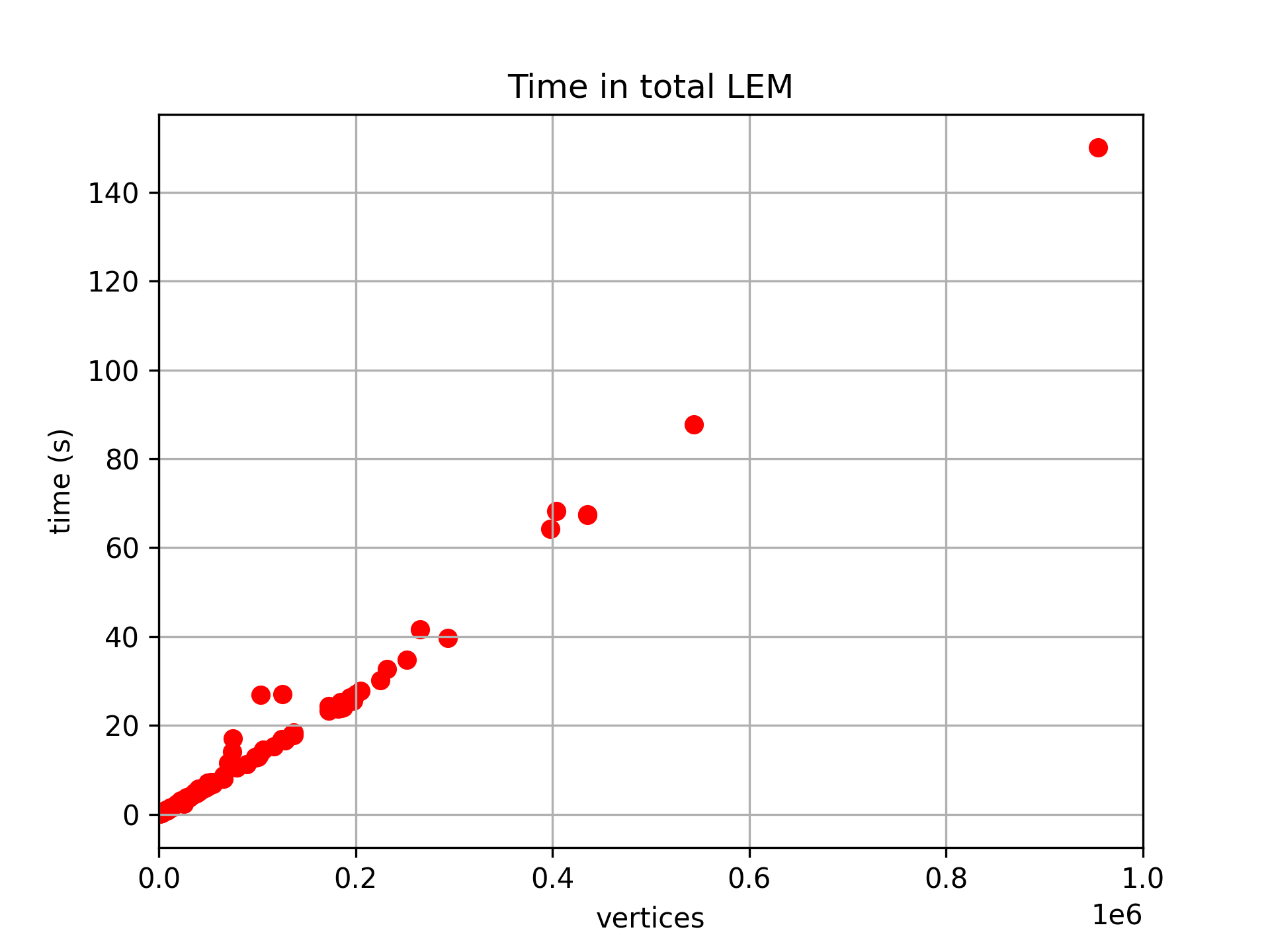
Remarkably, we find that the multilevel algorithm not only outperforms LSS by several orders of magnitude, but also that it seems to be less dependant on the underlying structure of the triangle meshes, giving what appears to be a slightly superlinear curve. This effect is even more pronounced when considering only the time to search for separators. Under assumptions about the degree of the graphs, we showed that searching was $O(1)$ for a single separator and $O(|V|)$ in total. This experiment seems to confirm that this assumption is fitting for classical input, as is the case with the triangle meshes of the Groningen Skeletonization Benchmark.

input	algorithm	coarsen (s)	search (s)	project (s)	pack (s)	total (s)
19465	LSS	-	25.8787	-	138.836	164.714
	LEM	1.20002	9.18989	9.410914	12.4392	26.8306
	LEMTS	1.21294	9.41457	14.851733	9.8696	26.5518
dragon	LSS	-	46615.4	-	20637.9	67255.9
	LEM	6.25851	49.6567	18.753684	3.42042	67.4554
	LEMTS	6.19801	50.2347	24.6420235	3.22507	69.4672
fertility	LSS	-	95.8574	-	42.1409	136.664
	LEM	0.234681	2.38572	0.7753682	0.0600592	3.03186
	LEMTS	0.244822	2.4305	1.8177949	0.0559833	3.44687
happy4	LSS	-	7646.21	-	15731.9	23379.2
	LEM	6.89638	49.6684	12.7328477	2.22244	64.2245
	LEMTS	6.93433	50.1269	16.0581559	1.75872	65.4557
horse	LSS	-	544.182	-	85.6915	628.3
	LEM	0.504898	5.10887	1.2762728	0.0669417	6.27845
	LEMTS	0.502791	5.17779	2.7604771	0.0542464	6.86374
neptune	LSS	-	56.296	-	62.8555	119.232
	LEM	0.312728	2.7382	1.0849813	0.230939	3.77785
	LEMTS	0.308124	2.76549	2.4149765	0.182575	4.22093

Table 2: Excerpt of running time measurements. In addition to measuring the total time, we also measure the time spent on each phase of the algorithm.

In Table 2 we show an excerpt of the running time measurements, including measurements of the phases of the algorithm. Here the vast gap in performance is clear, especially for dragon.ply, which is the largest input for which we have been able to run LSS, given a time frame of 20 hours. For this particular instance we achieve a running time that is almost a thousand times faster.

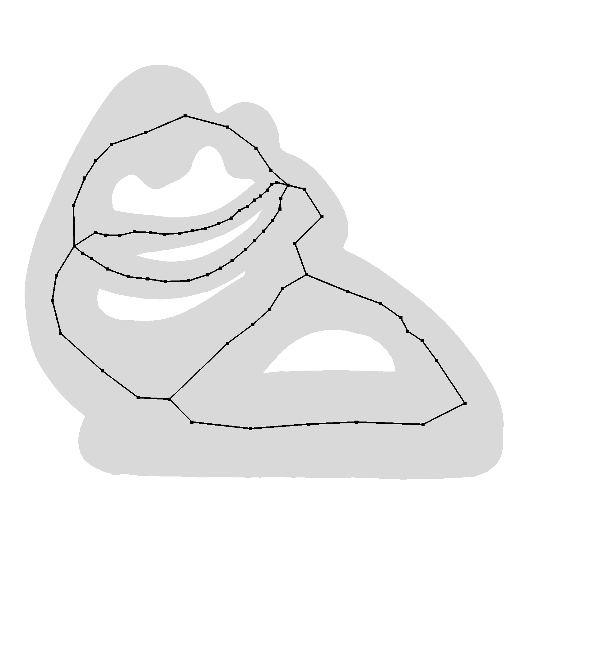
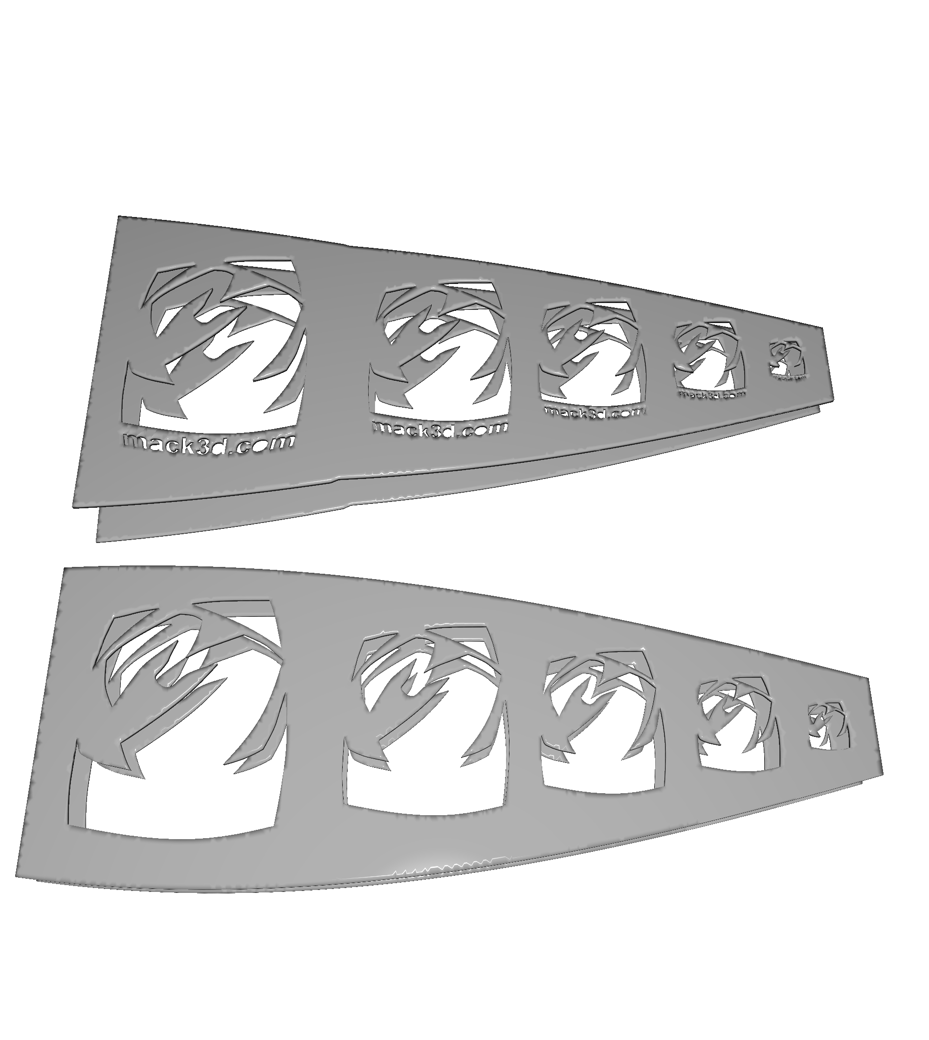
Of note is that LEMTS spends more time on projection, as expected, but less time on packing than LEM. As stated previously, the search for separators is often the dominating phase, however there are types of input for which this is not the case, as evidenced by 19465.ply. The mesh consists of flat sheets with small details engraved, as can be seen in Figure 11. For both LSS and the multilevel algorithms, a large portion of the time is spent on packing and projection. This can occur if the separators are generally small and plentiful, so that many of them may quickly be found. For 19465.ply these are particularly present around the imprinted text on the top sheets. It is worth noting that this would likely also be an example for which the structure of the input matters greatly for the running time of our multilevel algorithms.

Figure 11: The triangle mesh 19465.ply, where packing makes up a large portion of the running time for (all) local separator based skeletonization algorithms.

4 Conclusions and Future Work

We have proposed a multilevel algorithm for computing local separator-based curve skeletons, and shown that the approach is very efficient. We obtain a practical running time that appears near linear in the number of vertices of the input (see Figure 10) with up to thousandfold improvement in running time while not deteriorating the quality of the output substantially, if at all.

This type of running time improvement makes separator-based skeletonization applicable as a tool in biomedical image analysis, including frame-by-frame skeletonization of videos [3].

The application to video skeletonization motivates an unexplored line of related work, namely that of efficiently dynamically updating skeletons in a series of related shapes.

The multilevel approach offers great flexibility that has yet to be explored. It is easy to imagine coarsening schemes targeting specific structures of input, such as contracting clusters, rather than edges, on voxel input. These contraction schemes may provide new trade-offs between practical performance and skeleton quality.

When applying coarsening to scale-free graphs, as might be the case for data visualisation or areas of application that are not classical for skeletonization, we move into a domain known from the field of graph partitioning to cause trouble for matching contraction schemes [1]. It is interesting to see if the improved practical performance, and the applicability to any spatially embedded graph, opens up for new areas of application of skeletons.

Appendix A Time measurements

A.1 LSS

Table 3: Runtime measurements of LSS on the Groningen Skeletonization Benchmark

input	vertices	edges	search (s)	pack (s)	total (s)
17674	124998	375000	2210.77	1267.03	3478.68
18020	75122	225599	3.99153	45.1806	49.2553
19465	103351	310989	25.8787	138.836	164.714
20304	928	2790	0.241744	0.0326365	0.276727
20306	300	894	0.0331013	0.0025101	0.0371508
21362	1828	5862	1.35847	0.311618	1.67805
21464	9041	26817	0.855021	0.163493	1.02239
21747	2918	8766	0.0958573	0.0691565	0.167391
21788	23062	69132	34.9016	7.44311	42.3761
22081	3970	11934	0.892292	0.485193	1.3761
22290	944	2832	1.28241	0.0388288	1.32425
22601	12554	37704	2.08853	2.40571	4.50452
22669	28738	86208	199.372	25.7059	225.13
22701	52784	158346	7008.77	396.256	7405.48
22711	2820	8460	1.23153	0.252354	1.49249
22808	9640	28920	4.3411	0.936791	5.28941
22826	56143	168453	4086.67	867.461	4951.25
23091	4120	12354	5.90686	0.169803	6.0869
711_dente	9337	28005	34.1009	4.06142	38.1319
armadillo	172974	518916	11448.4	3543.65	14997.0
armadillo_vc	106289	318861	3204.65	1383.1	4592.3
asiandragon9a	231606	694743	5918.86	2587.44	8507.07
ballJoint	137062	411180	20924.2	1264.41	22189.5
bird2	11718	35148	21.1993	5.67294	26.8925
bird3	46866	140592	502.613	119.191	625.678
bird4	187458	562368	15499.6	2143.4	17643.8
bird	11718	35148	21.455	5.69072	27.1211
bmw2	125424	375531	592.198	723.553	1313.84
bmw	70536	211048	30.796	175.206	205.87
boeing	3975	10811	0.0979876	0.0840983	0.185436
brain2	294016	882048	52170.7	6002.66	58175.3
bunny	34834	104288	871.727	128.254	1000.12
bun_zipper	34834	104288	875.806	125.535	1004.16
bun_zipper_res2	8260	24480	25.3724	4.08634	29.4296
bun_zipper_res3	2000	5775	1.02591	0.143932	1.17524
bun_zipper_res4	518	1425	0.0644569	0.00645594	0.0730992
chicken_high	135142	405420	18539.4	2860.69	21424.2
cow10	181839	545481	10713.4	3048.3	13762.7
cow2	185730	557184	10498.4	3797.46	14222.4
cow3	252054	756090	46773.5	9664.54	56448.4
cube2	98306	294912	5827.69	35.6819	5863.63
dog	18114	54336	36.1876	13.7726	49.996
dragon	435680	1307182	46615.4	20637.9	67255.9
ele12a	50488	151470	430.976	107.081	538.198
ele_fine	173026	519060	12251.0	2526.92	14778.7
elk2	35062	105186	132.307	98.1348	230.095
fertility	24994	75000	95.8574	42.1409	136.664
frog	37225	111669	325.885	102.875	431.331
gargoyle	25002	75000	221.986	68.5221	291.185
grandpiano	2904	8136	0.132531	0.0202437	0.154685
happy4	397569	1190310	7646.21	15731.9	23379.2
heart	23062	69132	34.0533	6.79733	40.8846
heptoroid	79056	237294	66.3978	109.493	176.037
hh2	197245	591230	25040.0	4864.86	29869.8
hh	49374	147871	649.029	180.944	830.178
hht	53754	161109	1115.03	214.659	1329.94
hippo	40367	121082	355.525	132.543	489.036
horse3	193934	581796	15966.7	1511.87	17478.4
horse9	89400	268187	1071.45	387.892	1458.51
horse	48485	145449	544.182	85.6915	628.3
hound2	200463	600913	5757.82	2253.16	7977.3
hound	12578	37592	7.98674	3.63663	11.6414
human_hand	49374	147871	611.868	172.992	783.473
humerus	35002	105000	303.445	37.4675	340.978
ico	40962	122880	583.475	5.22691	588.763
kitten3	54838	164508	1491.24	389.112	1884.23
kitten	137098	411294	18429.4	3380.57	21810.9
lion2	65648	196696	1304.7	378.208	1683.55
lion	184738	550783	10751.5	2252.04	12985.5
lucy	100697	302085	2067.93	1035.66	3104.06
memento	26277	78825	100.99	36.0391	137.863
micscope2	265410	792121	1947.31	1260.84	3206.91
micscope	4146	12355	0.373911	0.0657359	0.443446
m	25631	71054	1.14553	1.7946	2.95392
mouse2	403652	1210944	44112.1	8690.16	52701.7
mouse	6311	18921	2.92597	0.691586	3.62578
neptune	28052	84168	56.296	62.8555	119.232
noisydino2	23370	69872	67.7212	30.5944	98.2667
noisydino8a	31497	94485	174.728	45.5758	219.857
noisydino	23370	69872	69.0721	30.8234	100.0
pig2	225282	675840	46042.1	8980.69	54639.5
pig	3522	10560	2.13615	0.539077	2.67718
pipe	2820	8460	1.20779	0.253799	1.46849
rcube2	98306	294912	6511.13	63.371	6574.24
rcube	24578	73728	281.882	3.76864	285.555
rhino2	128342	384790	2160.26	859.125	3025.39
rhino	8075	24058	3.43115	1.16439	4.60909
rockerArm2	43213	129639	792.765	118.601	911.377
rockerArm	40177	120531	629.687	62.2081	692.141
rotor	2328	7104	0.168337	0.0910922	0.261838
sacrum	204710	614226	9076.89	6283.98	15415.7
sandal2	40316	119568	27.8837	14.9089	42.8545
sandal3	22473	66039	35.9975	9.61242	45.7281
sandal	2636	7608	0.150706	0.0515755	0.205492
scapula	116930	350784	24658.3	3220.81	27880.1
screwdriver	27152	81450	635.749	48.1479	683.989
seabowl	45095	135303	569.478	119.554	688.461
ship1	2526	7220	0.0986438	0.0514934	0.152607
ship2	38122	113189	13.0851	20.6763	33.8212
ship3	74544	222199	56.9407	168.925	225.95
spider	4675	13929	0.524195	0.252	0.780605
tomgun2	65638	196496	82.568	78.9012	161.01
tomgun	4177	12305	0.388707	0.112197	0.504491
walleye2	49518	146582	309.593	81.8352	389.27
walleye	3343	9286	0.927982	0.128176	1.06049

A.2 LEM

Table 4: Runtime measurements of multilevel skeletonization using Light Edge Matchings on the Groningen Skeletonization Benchmark

input	vertices	edges	coarsen (s)	search (s)	project (s)	pack (s)	total (s)
17674	124998	375000	1.42035	13.4979	3.4347296	0.349129	16.8551
18020	75122	225599	0.713029	3.41843	6.5007303	10.2568	17.022
19465	103351	310989	1.20002	9.18989	9.410914	12.4392	26.8306
20304	928	2790	0.00472449	0.101381	0.022000955	0.000595655	0.119704
20306	300	894	0.00202366	0.0381954	0.012915355	0.000244554	0.0477475
21362	1828	5862	0.00957011	0.211413	0.03324375	0.00390133	0.249427
21464	9041	26817	0.0507172	0.605148	0.3172494	0.0488438	0.850748
21747	2918	8766	0.013928	0.16035	0.12938649	0.0353876	0.272814
21788	23062	69132	0.187331	2.19023	0.57236465	0.0442584	2.69455
22081	3970	11934	0.0225922	0.3726	0.10956878	0.0134095	0.463392
22290	944	2832	0.00453149	0.138593	0.018698548	0.000293809	0.154601
22601	12554	37704	0.0887529	0.95333	0.4130805	0.120493	1.35994
22669	28738	86208	0.274313	2.98669	0.51025489	0.0317114	3.5369
22701	52784	158346	0.473056	6.44374	0.28137197	0.00285178	7.15982
22711	2820	8460	0.0140559	0.318642	0.12283238	0.00448683	0.395761
22808	9640	28920	0.0650948	0.998223	0.20622033	0.0163558	1.17796
22826	56143	168453	0.512271	6.07731	1.0100605	0.0550804	7.14747
23091	4120	12354	0.0196667	0.455104	0.083162039	0.00300366	0.526664
711_dente	9337	28005	0.0641343	0.985219	0.22779954	0.0100632	9
armadillo	172974	518916	2.51794	19.0322	5.0844824	0.48021	24.3899
armadillo_vc	106289	318861	1.43063	11.3844	3.0456077	0.28918	14.4931
asiandragon10a	954227	2862226	14.0947	105.433	56.60956	7.17272	150.045
asiandragon9a	231606	694743	2.89486	23.9127	10.1410711	1.61975	32.5958
ballJoint	137062	411180	1.66799	15.7521	1.5901205	0.0301499	18.3389
bird2	11718	35148	0.092326	1.15743	0.35719044	0.0373765	1.44558
bird3	46866	140592	0.531434	4.70348	1.0330702	0.0722855	5.81154
bird4	187458	562368	2.23458	20.2136	2.6803021	0.134734	24.0237
bird	11718	35148	0.101527	1.13771	0.35191275	0.036676	1.42879
bmw2	125424	375531	1.53246	14.1645	7.991554	7.8399	26.958
bmw	70536	211048	0.699872	5.86059	3.613716	3.39631	11.5671
boeing	3975	10811	0.0174186	0.192201	0.140817	0.0562142	0.336693
brain2	294016	882048	3.57649	33.2128	5.1804536	0.266868	39.709
bunny	34834	104288	0.351915	3.78063	0.67709918	0.0480589	4.5399
bun_zipper	34834	104288	0.359259	3.79813	0.66139868	0.046271	4.5309
bun_zipper_res2	8260	24480	0.06046	0.86436	0.18984358	0.0197775	1.04349
bun_zipper_res3	2000	5775	0.0103474	0.197153	0.058296746	0.00757159	0.245245
bun_zipper_res4	518	1425	0.00334376	0.0538328	0.019278557	0.000693185	0.0692462
chicken_high	135142	405420	1.6475	15.2427	1.868914	0.041709	17.9348
cow10	181839	545481	2.13711	19.3315	4.4587347	0.226973	23.704
cow2	185730	557184	2.13695	18.7325	5.4557653	0.530463	23.8909
cow3	252054	756090	3.43701	28.0588	6.0824288	0.546523	34.7918
cow9	136988	410946	1.59892	14.5176	3.3032935	0.169401	17.7899
cube2	98306	294912	0.883138	11.2845	1.1164629	0.0178002	12.8058
dog	18114	54336	0.155731	1.79058	0.5426249	0.0481439	2.25427
dragon	435680	1307182	6.25851	49.6567	18.753684	3.42042	67.4554
dragon_vrip	435680	1307182	6.06857	49.8861	18.780025	3.46152	67.4061
dragon_vrip_res2	102112	303088	1.26637	10.3709	2.9057934	0.333104	13.3148
dragon_vrip_res3	24417	71126	0.230862	2.22082	0.7889312	0.0935623	2.91563
dragon_vrip_res4	5743	16431	0.0387931	0.47057	0.21363361	0.0264042	0.63171
ele12a	50488	151470	0.53858	5.01851	1.2827198	0.0729709	6.25953
ele_fine	173026	519060	2.29251	19.088	3.5553908	0.187306	23.2524
elk2	35062	105186	0.377056	3.53251	0.81446343	0.0563738	4.33083
fertility	24994	75000	0.234681	2.38572	0.7753682	0.0600592	3.03186
frog	37225	111669	0.362007	3.89609	1.0568452	0.153736	4.929
gargoyle	25002	75000	0.236856	2.72392	0.5215487	0.0393314	3.23942
grandpiano	2904	8136	0.0113828	0.175221	0.0559794	0.00671873	0.224557
happy4	397569	1190310	6.89638	49.6684	12.7328477	2.22244	64.2245
happy	543822	1631680	7.9146	66.7996	20.8506963	3.93399	87.752
heart	23062	69132	0.20292	2.16714	0.594186	0.0456437	2.69486
heptoroid	79056	237294	0.969235	6.84475	3.6109921	1.1477	10.5038
hh2	197245	591230	2.50199	20.7739	3.9906898	0.190638	25.4634
hh	49374	147871	0.517598	4.89417	1.366125	0.0889966	6.14942
hht	53754	161109	0.649063	5.36146	1.4218338	0.111029	6.83171
hippo	40367	121082	0.407343	4.28243	0.9159472	0.0617453	5.18609
horse3	193934	581796	2.46719	21.5099	4.4235634	0.160395	26.2848
horse9	89400	268187	1.02295	9.02118	2.4578347	0.153465	11.2601
horse	48485	145449	0.504898	5.10887	1.2762728	0.0669417	6.27845
hound2	200463	600913	2.21726	21.6746	5.4904756	0.53687	26.9504
hound	12578	37592	0.101115	1.15836	0.4332293	0.0557417	1.52113
human_hand	49374	147871	0.563042	4.92293	1.2874627	0.084787	6.17145
humerus	35002	105000	0.368269	3.59696	0.9222292	0.0306101	4.42637
ico	40962	122880	0.385356	4.70133	0.2181534	0.000810135	5.27336
kitten3	54838	164508	0.564621	5.72572	0.92238507	0.0368314	6.8351
kitten	137098	411294	1.63015	15.2895	1.9815453	0.0444201	18.0658
lion2	65648	196696	0.761081	6.9304	1.6788871	0.16808	8.70898
lion	184738	550783	2.2956	20.9184	3.6100428	0.288113	25.2353
lucy	100697	302085	1.20264	10.2482	2.5055618	0.201589	12.8405
memento	26277	78825	0.251496	2.57331	0.9146878	0.0917045	3.3258
micscope2	265410	792121	3.0882	29.8056	13.284129	3.11965	41.5345
micscope	4146	12355	0.020966	0.407153	0.0991788	0.0213976	0.502653
m	25631	71054	0.172642	1.23407	0.7839142	0.511338	2.2808
mouse2	403652	1210944	4.65876	47.6706	20.374639	7.6661	68.2746
mouse	6311	18921	0.0383902	0.652853	0.23409506	0.0430953	0.847976
neptune	28052	84168	0.312728	2.7382	1.0849813	0.230939	3.77785
noisydino2	23370	69872	0.235437	2.25831	0.7979447	0.0873257	2.91716
noisydino8a	31497	94485	0.319535	3.00893	0.9531643	0.0592822	3.78642
noisydino	23370	69872	0.223275	2.25698	0.8086116	0.0826377	2.92994
pig2	225282	675840	2.76833	24.2396	5.5608734	0.502856	30.1216
pig	3522	10560	0.0212906	0.286789	0.12774142	0.0229754	0.395927
pipe	2820	8460	0.0142335	0.321047	0.1244618	0.00482331	0.396382
rcube2	98306	294912	0.956272	11.0931	1.2481161	0.0166792	12.7712
rcube	24578	73728	0.184148	2.7447	0.28438118	0.00394089	3.11112
rhino2	128342	384790	1.48467	13.2432	3.2735371	0.26516	16.5302
rhino	8075	24058	0.0515384	0.736705	0.26798898	0.0347169	0.949532
rockerArm2	43213	129639	0.458789	4.56635	0.8497291	0.0225036	5.48141
rockerArm	40177	120531	0.40493	4.16544	0.8525191	0.0211871	5.00707
rotor	2328	7104	0.0119959	0.178435	0.09086232	0.0205675	0.257278
sacrum	204710	614226	2.81857	22.8123	3.8453268	0.223871	27.7257
sandal2	40316	119568	0.344412	3.9165	1.8148215	0.581826	5.66137
sandal3	22473	66039	0.203555	2.18896	0.782279	0.250619	3.01813
sandal	2636	7608	0.0122295	0.209453	0.10131738	0.0163152	0.288116
scapula	116930	350784	1.50627	12.7815	1.6220242	0.0559348	15.2969
screwdriver	27152	81450	0.256815	2.90263	0.54800159	0.022825	3.46602
seabowl	45095	135303	0.499152	4.7644	1.0131984	0.0813877	5.8672
ship1	2526	7220	0.0123951	0.149451	0.09039014	0.0201223	0.226589
ship2	38122	113189	0.339199	2.99193	1.5399452	0.589327	4.64253
ship3	74544	222199	0.862242	6.60576	3.8058408	4.91441	14.06
spider	4675	13929	0.0256434	0.364411	0.16410401	0.0562838	0.529353
tomgun2	65638	196496	0.651883	5.95249	2.2170524	0.441005	8.03167
tomgun	4177	12305	0.0214907	0.294542	0.1132001	0.0142692	0.384086
walleye2	49518	146582	0.471817	5.38596	1.4151858	0.535818	7.05759
walleye	3343	9286	0.0165995	0.314689	0.08863707	0.0095865	0.390043

A.3 LEMTS

Table 5: Runtime measurements of multilevel skeletonization using Light Edge Matchings and Thickened Separators on the Groningen Skeletonization Benchmark

input	vertices	edges	coarsen (s)	search (s)	project (s)	pack (s)	total (s)
17674	124998	375000	1.37288	13.8259	6.1536268	0.252363	18.094
18020	75122	225599	0.70643	3.50639	12.0219301	9.39802	18.3356
19465	103351	310989	1.21294	9.41457	14.851733	9.8696	26.5518
20304	928	2790	0.00476734	0.105907	0.051260507	0.000753875	0.135355
20306	300	894	0.00249888	0.0371973	0.024086454	0.000285874	0.0506875
21362	1828	5862	0.00991051	0.210066	0.09045887	0.00351191	0.270029
21464	9041	26817	0.0559211	0.619575	0.69601524	0.0423914	0.996912
21747	2918	8766	0.014122	0.172405	0.29007067	0.0304931	0.338011
21788	23062	69132	0.193463	2.16468	1.28154913	0.0426115	2.93941
22081	3970	11934	0.0226519	0.380269	0.25070048	0.0123173	0.519388
22290	944	2832	0.00448527	0.139352	0.038550872	0.000262215	0.160744
22601	12554	37704	0.0975062	0.987717	0.851674	0.100677	1.54694
22669	28738	86208	0.286316	3.0546	1.04230053	0.0200472	3.79582
22701	52784	158346	0.461819	6.42563	0.44446955	0.00207974	7.17059
22711	2820	8460	0.014311	0.323639	0.29059017	0.00287403	0.458739
22808	9640	28920	0.0634594	1.03166	0.41110239	0.00978584	1.27532
22826	56143	168453	0.519806	5.99483	2.4316612	0.0505605	7.60915
23091	4120	12354	0.0194701	0.469513	0.189625955	0.00240466	0.575799
711_dente	9337	28005	0.0686141	0.998655	0.53344135	0.00867415	1.30378
armadillo	172974	518916	2.46986	19.1877	9.4305278	0.327339	25.8982
armadillo_vc	106289	318861	1.39404	11.5249	6.2142442	0.214773	15.7169
asiandragon10a	954227	2862226	14.0653	105.332	83.178314	4.52812	155.153
asiandragon9a	231606	694743	2.8553	24.0592	16.917632	1.13746	34.8331
ballJoint	137062	411180	1.67507	15.6877	3.3411102	0.020369	18.9884
bird2	11718	35148	0.0805309	1.14146	0.84050036	0.0315955	1.59471
bird3	46866	140592	0.50282	4.73525	2.300044	0.0632088	6.22924
bird4	187458	562368	2.40017	20.3605	5.5991965	0.101529	25.3824
bird	11718	35148	0.093867	1.13195	0.81265529	0.0290167	1.57061
bmw2	125424	375531	1.51884	14.236	12.5885782	6.99201	28.1195
bmw	70536	211048	0.691096	5.92067	6.792073	2.90765	12.4277
boeing	3975	10811	0.0177992	0.196806	0.26577117	0.0488982	0.379375
brain2	294016	882048	3.57092	33.3187	8.5313576	0.242088	40.9286
bunny	34834	104288	0.363232	3.79656	1.37544507	0.039346	4.79618
bun_zipper	34834	104288	0.352807	3.84765	1.29270687	0.0410116	4.79398
bun_zipper_res2	8260	24480	0.0529122	0.878866	0.39589784	0.0167918	1.11783
bun_zipper_res3	2000	5775	0.010301	0.204269	0.12545401	0.00639514	0.279434
bun_zipper_res4	518	1425	0.00291506	0.0560733	0.04312842	0.000641622	0.0777027
chicken_high	135142	405420	1.60237	15.1774	3.5583817	0.0341168	18.4927
cow10	181839	545481	2.17961	19.437	8.4240864	0.175242	25.198
cow2	185730	557184	2.18291	19.0676	10.1746708	0.399085	25.9429
cow3	252054	756090	3.47587	28.2994	9.7904799	0.352022	36.1018
cow9	136988	410946	1.61981	14.357	6.3390355	0.144272	18.8167
cube2	98306	294912	0.888989	11.229	2.1635131	0.0130268	13.1271
dog	18114	54336	0.157395	1.79984	1.2110295	0.0413447	2.50017
dragon	435680	1307182	6.19801	50.2347	24.6420235	3.22507	69.4672
dragon_vrip	435680	1307182	6.15461	50.2762	25.094422	3.18479	69.3239
dragon_vrip_res2	102112	303088	1.19471	10.4939	4.989363	0.250379	14.0577
dragon_vrip_res3	24417	71126	0.230291	2.25178	1.39281064	0.0784439	3.1478
dragon_vrip_res4	5743	16431	0.037996	0.472024	0.42511038	0.0251362	0.713175
ele12a	50488	151470	0.53404	5.03626	2.7621634	0.0612321	6.73142
ele_fine	173026	519060	2.37588	19.1998	6.5201373	0.151195	24.563
elk2	35062	105186	0.381521	3.61194	1.60635173	0.0517945	4.71299
fertility	24994	75000	0.244822	2.4305	1.8177949	0.0559833	3.44687
frog	37225	111669	0.389961	3.90161	2.3034716	0.128718	5.41558
gargoyle	25002	75000	0.256161	2.72948	1.14925343	0.0307409	3.48302
grandpiano	2904	8136	0.0110036	0.17332	0.12285781	0.00571585	0.257232
happy4	397569	1190310	6.93433	50.1269	16.0581559	1.75872	65.4557
happy	543822	1631680	8.00506	66.9676	25.5106596	3.69385	89.5235
heart	23062	69132	0.173748	2.15771	1.35531625	0.0421466	2.93709
heptoroid	79056	237294	0.916259	6.89268	7.5853171	0.811116	11.527
hh2	197245	591230	2.47622	20.8036	7.4632686	0.141546	26.6708
hh	49374	147871	0.549817	4.90281	2.5108662	0.0721409	6.57878
hht	53754	161109	0.622599	5.42222	2.9174229	0.0837678	7.35467
hippo	40367	121082	0.448026	4.35356	2.0381683	0.0544027	5.67898
horse3	193934	581796	2.42718	21.594	8.339175	0.119572	27.6041
horse9	89400	268187	0.997401	8.90845	5.3143602	0.116107	12.1142
horse	48485	145449	0.502791	5.17779	2.7604771	0.0542464	6.86374
hound2	200463	600913	2.27636	21.788	10.7396585	0.43615	28.8567
hound	12578	37592	0.104805	1.18453	0.9476307	0.05026	1.72187
human_hand	49374	147871	0.540201	4.91299	2.5593691	0.0726399	6.53822
humerus	35002	105000	0.353858	3.68623	1.8732058	0.0239917	4.85062
ico	40962	122880	0.367218	4.71673	0.2244697	0.000601861	5.29382
kitten3	54838	164508	0.556148	5.78029	1.6071862	0.0306763	7.14854
kitten	137098	411294	1.64587	15.2583	3.3345443	0.0400726	18.4326
lion2	65648	196696	0.697095	6.87126	3.0194409	0.141892	8.98981
lion	184738	550783	2.26651	21.0421	6.0643192	0.200554	26.2529
lucy	100697	302085	1.15179	10.2905	4.5310875	0.166912	13.5347
memento	26277	78825	0.2703	2.57669	2.1355263	0.0789704	3.78361
micscope2	265410	792121	2.99505	29.5575	21.684033	2.22369	43.0669
micscope	4146	12355	0.0204097	0.403439	0.19514139	0.0205848	0.536987
m	25631	71054	0.185894	1.24326	1.4135061	0.40673	2.45396
mouse2	403652	1210944	4.61188	47.9421	31.821861	5.08602	69.811
mouse	6311	18921	0.0384411	0.662394	0.52321536	0.0358318	0.972776
neptune	28052	84168	0.308124	2.76549	2.4149765	0.182575	4.22093
noisydino2	23370	69872	0.236898	2.26549	1.7555544	0.0726686	3.26698
noisydino8a	31497	94485	0.30512	3.03009	2.0297282	0.0489356	4.20738
noisydino	23370	69872	0.239336	2.25737	1.7335359	0.0699845	3.25217
pig2	225282	675840	2.69757	24.441	10.4396925	0.39946	31.8039
pig	3522	10560	0.0200319	0.306373	0.29780277	0.0225411	0.477153
pipe	2820	8460	0.0143922	0.328995	0.28918437	0.00284439	0.457443
rcube2	98306	294912	0.975693	11.1107	2.1495174	0.0140855	13.1207
rcube	24578	73728	0.186935	2.79348	0.52618835	0.00214423	3.2175
rhino2	128342	384790	1.44105	13.5052	6.3808746	0.215573	17.6696
rhino	8075	24058	0.0539976	0.736505	0.57325506	0.0331398	1.06554
rockerArm2	43213	129639	0.463274	4.54615	1.99677959	0.01904	5.82642
rockerArm	40177	120531	0.392621	4.1855	1.82895265	0.0141119	5.34244
rotor	2328	7104	0.0118651	0.181803	0.17895838	0.0197181	0.2917
sacrum	204710	614226	2.73006	22.9159	6.8929541	0.177687	28.8622
sandal2	40316	119568	0.346656	4.06497	3.8798318	0.430996	6.39904
sandal3	22473	66039	0.191946	2.23852	1.6852481	0.210204	3.33725
sandal	2636	7608	0.0121956	0.212033	0.1907273	0.0166909	0.325527
scapula	116930	350784	1.51976	12.8966	3.0576659	0.0464446	15.87
screwdriver	27152	81450	0.246062	2.97392	1.08712076	0.0162187	3.69605
seabowl	45095	135303	0.470481	4.82754	2.1035185	0.0734754	6.33133
ship1	2526	7220	0.0122548	0.160322	0.17935572	0.0204451	0.27645
ship2	38122	113189	0.328891	3.04911	3.2117841	0.473475	5.20903
ship3	74544	222199	0.866528	6.60474	7.1166426	3.51893	13.8594
spider	4675	13929	0.0240519	0.385193	0.3277413	0.0539168	0.607832
tomgun2	65638	196496	0.65928	6.10129	4.5972224	0.347689	8.98068
tomgun	4177	12305	0.0210423	0.299244	0.23149471	0.0134622	0.434965
walleye2	49518	146582	0.450784	5.3944	2.9724058	0.528678	7.53503
walleye	3343	9286	0.015999	0.311624	0.21487931	0.00890859	0.43915

Appendix B Skeleton Comparisons

B.1 LSS and LEM

Table 6: Comparison between skeletons generated by LSS and LEM. The metrics denoted by $\Delta$ are relative to the skeletons of LSS, with negative values implying that LSS has more vertices, leafs, branches etc. Here $H($LEM,LSS$)$ denotes the directed Hausdorff distance between LEM and LSS, divided by the radius of a bounding sphere, and vice versa.

input	$\Delta$vertices	$\Delta$leafs	$\Delta$branches	$\Delta$genus	$H($LEM,LSS$)$	$H($LSS,LEM$)$
17674	-214	-6	-7	-2	0.242987	0.136002
18020	-132	0	2	0	0.0267864	0.0265365
19465	-563	-3	-35	2	0.0437028	0.0415616
20304	0	6	-1	-2	0.534996	0.365925
20306	1	1	0	0	0.13103	0.137122
21362	1	1	0	0	0.138338	0.0941336
21464	-94	-1	-1	0	0.0287383	0.0848934
21747	-4	0	0	0	0.0232842	0.0247181
21788	-39	-4	3	0	0.331518	0.253539
22081	-41	2	2	0	0.0191042	0.0364621
22290	-4	-8	2	-1	0.724273	0.584943
22601	-12	-4	6	0	0.0448619	0.0455526
22669	-106	1	1	0	0.144748	0.123809
22701	-4	2	-1	0	0.595045	0.353578
22711	-10	0	0	0	0.0529444	0.0371701
22808	-76	0	0	0	0.0371294	0.0360032
22826	-35	16	1	-4	0.263343	0.257184
23091	-29	0	-1	0	0.396678	0.28389
711_dente	-10	-3	-2	0	0.474553	0.201984
armadillo	-149	-17	-6	0	0.220078	0.165342
armadillo_vc	-130	-19	-10	0	0.249026	0.0830985
asiandragon10a	485	63	27	1	-	-
asiandragon9a	-303	-27	-3	0	0.146472	0.0809961
ballJoint	-34	-9	-5	0	0.335091	0.128461
bird2	-40	-2	-2	0	0.0911887	0.0434792
bird3	-66	-6	-2	0	0.102782	0.0483936
bird4	-99	-6	-2	0	0.131071	0.0457664
bird	-35	-1	-1	0	0.064136	0.0591958
bmw2	-61	-5	5	0	0.181548	0.165533
bmw	-96	-10	0	0	0.140737	0.13919
boeing	-6	4	2	0	0.0700192	0.0958734
brain2	-91	-51	-11	2	0.380483	0.274007
bunny	-35	-13	-2	0	0.371084	0.218552
bun_zipper_res2	-23	-5	-5	-1	0.309635	0.228842
bun_zipper_res3	-10	-2	-1	-1	0.387004	0.224203
bun_zipper_res4	-1	0	0	0	0.237761	0.19944
bun_zipper	-34	-12	-2	0	0.366736	0.184346
chicken_high	-65	-25	-10	0	0.352596	0.128001
cow10	-204	-2	0	0	0.131613	0.0956342
cow2	-213	-1	0	0	0.0974546	0.0992171
cow3	-200	1	-2	0	0.161176	0.118553
cow9	145	15	3	1	-	-
cube2	-36	-1	-1	0	0.545168	0.322115
dog	-58	-9	-4	0	0.0901815	0.058035
dragon	-277	-35	-31	-2	0.221926	0.124984
dragon_vrip_res2	390	174	51	1	-	-
dragon_vrip_res3	307	152	39	1	-	-
dragon_vrip_res4	152	65	24	1	-	-
dragon_vrip	777	222	71	23	-	-
ele12a	-87	-3	-1	0	0.185378	0.123558
ele_fine	-196	-4	-6	0	0.187097	0.157745
elk2	-53	-1	-2	0	0.212646	0.251487
fertility	-46	-3	-1	0	0.273804	0.0874419
frog	-86	-2	0	0	0.22128	0.141774
gargoyle	-56	-19	-10	0	0.318482	0.147751
grandpiano	-4	0	0	0	0.164264	0.190796
happy4	-589	-409	-21	-100	0.199295	0.0887277
happy	982	308	58	44	-	-
heart	-41	-7	5	0	0.336127	0.243949
heptoroid	-245	0	0	0	0.0705061	0.068063
hh2	-100	-1	-2	0	0.193822	0.189663
hh	-61	0	-3	0	0.17783	0.141936
hht	-86	1	1	0	0.149574	0.174906
hippo	-80	-17	-12	0	0.20746	0.153264
horse3	-190	-2	-3	0	0.130538	0.123331
horse9	-148	-2	-1	0	0.110968	0.101046
horse	-95	-1	-1	0	0.112222	0.111066
hound2	-88	-20	1	0	0.17887	0.0557737
hound	-25	0	2	-1	0.0854626	0.0731542
human_hand	-64	-3	-1	0	0.181229	0.0866464
humerus	-60	-4	-1	0	0.0959782	0.0774577
kitten3	-25	-5	0	0	0.234016	0.267631
kitten	-46	-8	-1	0	0.26524	0.197679
lion2	-179	-56	-17	0	0.171686	0.118093
lion	-246	-60	-18	1	0.206408	0.10091
lucy	-175	-93	-13	0	0.163102	0.133512
memento	-72	-1	-2	0	0.326454	0.226977
micscope2	-1447	1	-5	0	0.0999958	0.410087
micscope	-6	-6	-5	2	0.0163587	0.526192
mouse2	-202	-19	-5	0	0.133177	0.0925803
mouse	-2	-3	1	0	0.0942147	0.110964
m	44	15	6	1	0.0580312	0.181962
neptune	-73	-16	-5	0	0.200924	0.0508065
noisydino2	-59	-10	-7	0	0.0858338	0.0586712
noisydino8a	-63	-3	-3	0	0.0876304	0.0788599
noisydino	-51	-6	-5	0	0.0871886	0.0806523
pig2	-233	-3	-1	0	0.281781	0.13851
pig	-5	1	1	0	0.136812	0.185151
pipe	-9	0	0	0	0.0608525	0.0367033
rcube2	-26	-2	-2	0	0.82234	0.37449
rcube	-35	-1	-1	0	0.552556	0.481529
rhino2	-190	-52	-20	0	0.285996	0.107248
rhino	-28	-13	-6	0	0.207169	0.124026
rockerArm2	-46	-1	-1	0	0.254169	0.157712
rockerArm	-33	-1	-1	0	0.262787	0.147716
rotor	-29	3	1	0	0.0792849	0.0977375
sacrum	-147	-22	-12	-4	0.408094	0.169373
sandal2	-315	5	-6	-2	0.136338	0.0763513
sandal3	-95	16	-11	-6	0.148504	0.0690598
sandal	6	4	4	-2	0.102921	0.0923182
scapula	-81	-10	-9	0	0.325198	0.170676
screwdriver	-55	-2	-1	0	0.19814	0.0929329
seabowl	-88	-19	-5	-1	0.366275	0.173513
ship1	2	-9	6	4	0.248314	0.187957
ship2	-79	2	-1	-6	0.196807	0.20017
ship3	-167	13	-5	-5	0.166875	0.23599
spider	12	-2	-2	0	0.0914775	0.0515585
tomgun2	-89	51	-9	-2	0.0771206	0.0655649
tomgun	3	-5	-2	0	0.045953	0.0647683
walleye2	-49	0	4	-1	0.133166	0.041185
walleye	-1	-10	3	0	0.212548	0.0931524

B.2 LSS and LEMTS

Table 7: Comparison between skeletons generated by LSS and LEM. The metrics denoted by $\Delta$ are relative to the skeletons of LSS, with negative values implying that LSS has more vertices, leafs, branches etc. Here $H($LEMTS,LSS$)$ denotes the directed Hausdorff distance between LEMTS and LSS, divided by the radius of a bounding sphere, and vice versa

input	$\Delta$vertices	$\Delta$leafs	$\Delta$branches	$\Delta$genus	$H($LEMTS,LSS$)$	$H($LSS,LEMTS$)$
17674	-173	-9	-7	0	0.255787	0.140655
18020	-141	0	8	0	0.0369842	0.0388943
19465	-416	11	-24	3	0.0355444	0.0382796
20304	1	9	-2	-2	0.331099	0.371398
20306	2	1	0	0	0.141557	0.175343
21362	3	3	0	0	0.0831445	0.205519
21464	-37	-1	-1	0	0.0287383	0.0847032
21747	-3	0	0	0	0.0122935	0.0121544
21788	-21	-1	4	0	0.316065	0.241109
22081	-36	1	0	0	0.0184155	0.0292149
22290	-3	-9	1	-1	0.701622	0.593782
22601	-13	-8	3	0	0.0505034	0.041482
22669	-95	1	1	0	0.107136	0.18301
22701	-1	2	0	0	0.47311	0.324789
22711	-4	0	0	0	0.0496445	0.0350731
22808	-79	0	0	0	0.0509979	0.0508452
22826	-23	17	2	-2	0.142766	0.179552
23091	-28	0	0	0	0.194078	0.142976
711_dente	-9	-4	-2	0	0.461223	0.304697
armadillo	-108	-17	-3	0	0.218784	0.145593
armadillo_vc	-95	-17	-4	0	0.256114	0.149753
asiandragon10a	664	63	33	1	-	-
asiandragon9a	-204	-26	0	0	0.149798	0.0878272
ballJoint	-30	-9	-5	0	0.345708	0.107102
bird2	-24	0	1	0	0.0646921	0.0660722
bird3	-45	-6	-2	0	0.106499	0.0485063
bird4	-79	-6	-1	0	0.154138	0.0779006
bird	-29	-1	-1	0	0.0540386	0.049263
bmw2	-49	-9	11	3	0.204429	0.154384
bmw	-25	17	22	1	0.143202	0.139063
boeing	1	21	2	-9	0.0911128	0.0844408
brain2	-71	-50	-5	-1	0.442813	0.243605
bunny	-29	-10	-1	-1	0.381509	0.185589
bun_zipper_res2	-21	-6	-4	0	0.332003	0.206632
bun_zipper_res3	-10	-4	-2	0	0.353706	0.228834
bun_zipper_res4	0	1	0	0	0.18867	0.390443
bun_zipper	-35	-10	-3	-1	0.373315	0.186499
chicken_high	-56	-25	-10	0	0.345959	0.104203
cow10	-129	-2	0	0	0.132759	0.0965579
cow2	-132	-1	1	0	0.145401	0.187487
cow3	-126	0	0	0	0.188258	0.10453
cow9	217	15	8	1	-	-
cube2	-35	-1	-1	0	0.502338	0.334772
dog	-44	-9	-4	0	0.0854458	0.072164
dragon	-222	-36	-26	-3	0.255397	0.11414
dragon_vrip_res2	412	170	52	1	-	-
dragon_vrip_res3	323	155	44	1	-	-
dragon_vrip_res4	149	64	22	1	-	-
dragon_vrip	824	227	74	19	-	-
ele12a	-54	-3	0	0	0.174368	0.182298
ele_fine	-158	-4	-3	0	0.202761	0.163576
elk2	-35	-1	-1	0	0.189953	0.170198
fertility	-30	-3	-1	0	0.240033	0.165239
frog	-65	-2	2	0	0.213764	0.176573
gargoyle	-54	-21	-11	0	0.379466	0.147014
grandpiano	0	2	0	0	0.129011	0.162077
happy4	-560	-384	-22	-99	0.160472	0.100934
happy	1020	334	57	41	-	-
heart	-21	-2	5	0	0.326899	0.232986
heptoroid	-132	0	2	0	0.0975426	0.0763043
hh2	-70	2	-1	0	0.19555	0.170324
hh	-44	0	0	0	0.169264	0.116556
hht	-60	1	-1	0	0.177192	0.16365
hippo	-64	-13	-6	0	0.19232	0.132381
horse3	-125	0	-1	0	0.119945	0.110306
horse9	-96	-2	-1	0	0.113884	0.103661
horse	-66	-2	-2	0	0.0883287	0.0851157
hound2	-54	-16	2	0	0.190078	0.0818325
hound	-22	-3	1	0	0.0846057	0.0696693
human_hand	-46	-2	-1	0	0.147885	0.0809871
humerus	-37	-6	-3	0	0.112056	0.0725165
kitten3	-18	-5	0	0	0.221592	0.306183
kitten	-29	-5	1	0	0.271288	0.201393
lion2	-147	-55	-10	0	0.170177	0.121737
lion	-203	-59	-19	1	0.209613	0.102484
lucy	-173	-95	-17	0	0.181825	0.147681
memento	-47	-1	-2	0	0.335567	0.234729
micscope2	-1188	7	5	0	0.107463	0.514925
micscope	-8	0	-6	-1	0.0139525	0.73694
mouse2	-100	-15	2	0	0.122646	0.079835
mouse	-3	-4	1	0	0.105162	0.14296
m	82	44	13	-1	0.0563222	0.19182
neptune	-51	-15	-1	0	0.225756	0.0516766
noisydino2	-59	-10	-6	0	0.0938331	0.0921727
noisydino8a	-49	-3	-2	0	0.0855693	0.0707761
noisydino	-49	-4	-5	0	0.0789956	0.073725
pig2	-141	-3	0	0	0.275567	0.124252
pig	-8	1	0	0	0.124846	0.152941
pipe	-4	0	0	0	0.0496445	0.0350761
rcube2	-24	-1	-1	0	0.6971	0.583039
rcube	-37	-2	-2	0	0.487541	0.225971
rhino2	-144	-46	-18	0	0.240027	0.211737
rhino	-14	-7	-2	0	0.398101	0.126916
rockerArm2	-36	0	0	0	0.240848	0.250368
rockerArm	-25	-1	-1	0	0.212998	0.0977234
rotor	-23	7	5	0	0.0882883	0.0897212
sacrum	-126	-28	-8	-1	0.427385	0.157824
sandal2	-241	10	-4	-2	0.0668588	0.0665051
sandal3	-73	17	-10	-6	0.0947857	0.0566952
sandal	7	4	3	-2	0.123407	0.0806454
scapula	-65	-9	-8	0	0.332365	0.244491
screwdriver	-36	-1	0	0	0.203488	0.104393
seabowl	-77	-20	-4	-1	0.32748	0.206797
ship1	2	-6	1	2	0.215595	0.182269
ship2	-74	1	1	1	0.170628	0.168638
ship3	-164	-1	-4	-2	0.151358	0.160943
spider	31	-2	-2	0	0.0956197	0.0793788
tomgun2	-33	75	7	-2	0.0602913	0.032726
tomgun	10	-5	1	1	0.0462826	0.0491785
walleye2	-16	13	18	-3	0.150528	0.0501536
walleye	-2	-11	2	0	0.212825	0.0933191

Appendix C On Computing Local Separators

C.1 Dynamic Connectivity

To speed up the check for disconnection of the front when computing local separators, Bærentzen and Rotenberg suggests [5] using a dynamic connectivity data structure such as the one by Holm, de Lichtenberg and Thorup [16]. This data structure uses a hierarchy of Euler Tour Forests to give $O(\log^{2}|V|)$ amortized update and query time. In practice, it can be beneficial to stop using the hierarchy, once forests reach small size.

Figure 12: Running time of local separator skeletonization using increasing thresholds in the dynamic connectivity data structure. The tested input wsm1 is a mesh while wsv is a voxel grid representing the same shape.

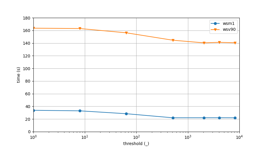
We have implemented the structure, integrated it into the local separator skeletonization implementation of GEL and tested the performance for various thresholds for when to stop using the hierarchy. The measurements are presented in Figure 12. What we found is that the performance increases with the size of the threshold, up to a point where the entirety of the hierarchy exists on a single level. In this manner, the data structure simply reduces to maintaining an augmented Euler Tour Forest. This is likely due to the specific access pattern when computing local separators, where edges are inserted and removed only once in a manner where separators that were inserted early are often removed before those inserted recently.

Figure 13: Running times of local separator skeletonization without (old) and with (dyn) the use of dynamic connectivity. Left shows performance on meshes while right shows performance on voxels.

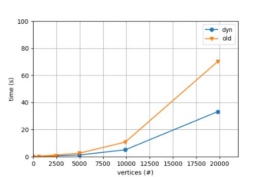
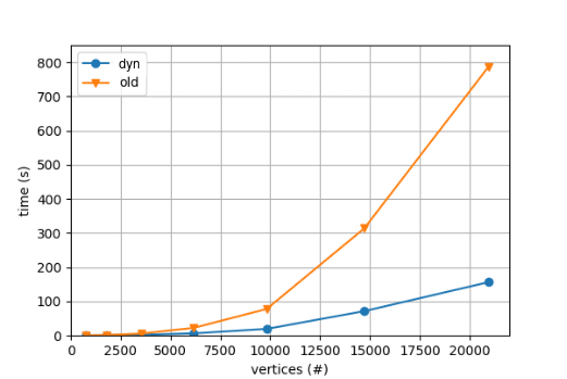
We also examine and compare running times when using dynamic connectivity. In Figure 13 we compare the old method to the one using dynamic connectivity (dyn), and find that for both meshes and voxels there is a large improvement. It is worth noting that this improvement seems even greater for voxels.

C.2 Analysis of Minimising Separators

Given a local separator $\Sigma$ on a graph $G$ with $n$ vertices and $m$ edges we describe the time it takes to minimise $\Sigma$.

To smooth the attribute of a vertex, we have to consider the positions of that vertex’ neighbours, giving a time complexity on the order of the degree of the vertex. Since we do this for every vertex in the separator, the time is proportional to the sum of degrees of vertices in the separator which is then bounded by two times the number of edges in the neighbourhood of the separator, by the handshaking lemma. Let $m^{\prime}$ be the number of edges in the closed neighbourhood of $\Sigma$, the time to smooth is then $O(m^{\prime})$. Computing the heuristic after smoothing takes $O(1)$ time per vertex, totalling in $O(|\Sigma|)$ time. We then sort the vertices according to the smoothed attributes in $O(|\Sigma|\log|\Sigma|)$ time.

After sorting we iteratively move vertices from the separator to front components. In the worst case we move only a constant number of vertices in each iteration, resulting in $O(|\Sigma|)$ total iterations over a collection of $O(|\Sigma|)$ vertices. Assuming we can move a vertex from one set to another in constant time, this step takes $O(|\Sigma|^{2})$ time.

The total time it takes is then $O(|\Sigma|^{2}+m^{\prime})$. Once again we can pessimistically bound both sets on the size of the graph s.t. $|\Sigma|=O(n)$ and $m^{\prime}=O(m)$ but also $m=O(n^{2})$. The time it takes to shrink a single separator is then bounded by $O(n^{2})$ in the worst case.

References

- [1] Amine Abou-Rjeili and George Karypis. Multilevel algorithms for partitioning power-law graphs. In 20th International Parallel and Distributed Processing Symposium (IPDPS 2006), Proceedings, 25-29 April 2006, Rhodes Island, Greece. IEEE, 2006. doi:10.1109/IPDPS.2006.1639360.
- [2] Nina Amenta, Sunghee Choi, and Ravi Krishna Kolluri. The power crust. In David C. Anderson and Kunwoo Lee, editors, Sixth ACM Symposium on Solid Modeling and Applications, Sheraton Inn, Ann Arbor, Michigan, USA, June 4-8, 2001, pages 249–266. ACM, 2001. doi:10.1145/376957.376986.
- [3] Kasra Arnavaz, Oswin Krause, Kilian Zepf, Jakob Andreas Bærentzen, Jelena M. Krivokapic, Silja Heilmann, Pia Nyeng, and Aasa Feragen. Quantifying topology in pancreatic tubular networks from live imaging 3d microscopy. Machine Learning for Biomedical Imaging, 1, 2022. URL: https://melba-journal.org/papers/2022:015.html.
- [4] Oscar Kin-Chung Au, Chiew-Lan Tai, Hung-Kuo Chu, Daniel Cohen-Or, and Tong-Yee Lee. Skeleton extraction by mesh contraction. ACM Trans. Graph., 27(3):44, 2008. doi:10.1145/1360612.1360643.
- [5] Andreas Bærentzen and Eva Rotenberg. Skeletonization via local separators. ACM Trans. Graph., 40(5):187:1–187:18, 2021. doi:10.1145/3459233.
- [6] Silvia Biasotti, Leila De Floriani, Bianca Falcidieno, Patrizio Frosini, Daniela Giorgi, Claudia Landi, Laura Papaleo, and Michela Spagnuolo. Describing shapes by geometrical-topological properties of real functions. ACM Comput. Surv., 40(4):12:1–12:87, 2008. doi:10.1145/1391729.1391731.
- [7] Silvia Biasotti, Daniela Giorgi, Michela Spagnuolo, and Bianca Falcidieno. Reeb graphs for shape analysis and applications. Theor. Comput. Sci., 392(1-3):5–22, 2008. doi:10.1016/j.tcs.2007.10.018.
- [8] Angela Brennecke and Tobias Isenberg. 3d shape matching using skeleton graphs. In Thomas Schulze, Stefan Schlechtweg, and Volkmar Hinz, editors, Simulation und Visualisierung 2004 (SimVis 2004) 4-5 März 2004, Magdeburg, pages 299–310. SCS Publishing House e.V., 2004. URL: http://wwwisg.cs.uni-magdeburg.de/graphik/pub/files/Brennecke_2004_3SM.pdf.
- [9] Aydin Buluç, Henning Meyerhenke, Ilya Safro, Peter Sanders, and Christian Schulz. Recent advances in graph partitioning. In Lasse Kliemann and Peter Sanders, editors, Algorithm Engineering - Selected Results and Surveys, volume 9220 of Lecture Notes in Computer Science, pages 117–158. Springer International Publishing, 2016. doi:10.1007/978-3-319-49487-6\_4.
- [10] Junjie Cao, Andrea Tagliasacchi, Matt Olson, Hao Zhang, and Zhixun Su. Point cloud skeletons via laplacian based contraction. In SMI 2010, Shape Modeling International Conference, Aix en Provence, France, June 21-23 2010, pages 187–197. IEEE Computer Society, 2010. doi:10.1109/SMI.2010.25.
- [11] Nicu D. Cornea, Deborah Silver, and Patrick Min. Curve-skeleton properties, applications, and algorithms. IEEE Trans. Vis. Comput. Graph., 13(3):530–548, 2007. doi:10.1109/TVCG.2007.1002.
- [12] Tamal K. Dey and Jian Sun. Defining and computing curve-skeletons with medial geodesic function. In Alla Sheffer and Konrad Polthier, editors, Proceedings of the Fourth Eurographics Symposium on Geometry Processing, Cagliari, Sardinia, Italy, June 26-28, 2006, volume 256 of ACM International Conference Proceeding Series, pages 143–152. Eurographics Association, 2006. doi:10.2312/SGP/SGP06/143-152.
- [13] William Harvey, Yusu Wang, and Rephael Wenger. A randomized O(m log m) time algorithm for computing reeb graphs of arbitrary simplicial complexes. In David G. Kirkpatrick and Joseph S. B. Mitchell, editors, Proceedings of the 26th ACM Symposium on Computational Geometry, Snowbird, Utah, USA, June 13-16, 2010, pages 267–276. ACM, 2010. doi:10.1145/1810959.1811005.
- [14] M. Sabry Hassouna and Aly A. Farag. Variational curve skeletons using gradient vector flow. IEEE Trans. Pattern Anal. Mach. Intell., 31(12):2257–2274, 2009. doi:10.1109/TPAMI.2008.271.
- [15] Bruce Hendrickson and Robert W. Leland. A multi-level algorithm for partitioning graphs. In Sidney Karin, editor, Proceedings Supercomputing ’95, San Diego, CA, USA, December 4-8, 1995, page 28. ACM, 1995. doi:10.1145/224170.224228.
- [16] Jacob Holm, Kristian de Lichtenberg, and Mikkel Thorup. Poly-logarithmic deterministic fully-dynamic algorithms for connectivity, minimum spanning tree, 2-edge, and biconnectivity. J. ACM, 48(4):723–760, 2001. doi:10.1145/502090.502095.
- [17] Hui Huang, Shihao Wu, Daniel Cohen-Or, Minglun Gong, Hao Zhang, Guiqing Li, and Baoquan Chen. L-medial skeleton of point cloud. ACM Trans. Graph., 32(4):65:1–65:8, 2013. doi:10.1145/2461912.2461913.
- [18] Rasmus E. Christensen J. Andreas Bærentzen and Emil T. Gæde. Gel. https://github.com/Sgelet/GEL, 2022.
- [19] Andrei C. Jalba, Jacek Kustra, and Alexandru C. Telea. Surface and curve skeletonization of large 3d models on the GPU. IEEE Trans. Pattern Anal. Mach. Intell., 35(6):1495–1508, 2013. doi:10.1109/TPAMI.2012.212.
- [20] Wei Jiang, Kai Xu, Zhi-Quan Cheng, Ralph R. Martin, and Gang Dang. Curve skeleton extraction by coupled graph contraction and surface clustering. Graph. Model., 75(3):137–148, 2013. doi:10.1016/j.gmod.2012.10.005.
- [21] George Karypis and Vipin Kumar. Analysis of multilevel graph partitioning. In Sidney Karin, editor, Proceedings Supercomputing ’95, San Diego, CA, USA, December 4-8, 1995, page 29. ACM, 1995. doi:10.1145/224170.224229.
- [22] Mattia Natali, Silvia Biasotti, Giuseppe Patanè, and Bianca Falcidieno. Graph-based representations of point clouds. Graph. Model., 73(5):151–164, 2011. doi:10.1016/j.gmod.2011.03.002.
- [23] Valerio Pascucci, Giorgio Scorzelli, Peer-Timo Bremer, and Ajith Mascarenhas. Robust on-line computation of reeb graphs: simplicity and speed. ACM Trans. Graph., 26(3):58, 2007. doi:10.1145/1276377.1276449.
- [24] Diane Perchet, Catalin I. Fetita, and Françoise J. Prêteux. Advanced navigation tools for virtual bronchoscopy. In Edward R. Dougherty, Jaakko Astola, and Karen O. Egiazarian, editors, Image Processing: Algorithms and Systems III, San Jose, California, USA, January 18, 2004, volume 5298 of SPIE Proceedings, pages 147–158. SPIE, 2004. doi:10.1117/12.533096.
- [25] Dennie Reniers, Jarke J. van Wijk, and Alexandru C. Telea. Computing multiscale curve and surface skeletons of genus 0 shapes using a global importance measure. IEEE Trans. Vis. Comput. Graph., 14(2):355–368, 2008. doi:10.1109/TVCG.2008.23.
- [26] Andrea Tagliasacchi, Ibraheem Alhashim, Matt Olson, and Hao Zhang. Mean curvature skeletons. Comput. Graph. Forum, 31(5):1735–1744, 2012. doi:10.1111/j.1467-8659.2012.03178.x.
- [27] Andrea Tagliasacchi, Thomas Delamé, Michela Spagnuolo, Nina Amenta, and Alexandru C. Telea. 3d skeletons: A state-of-the-art report. Comput. Graph. Forum, 35(2):573–597, 2016. doi:10.1111/cgf.12865.
- [28] Alexandru C. Telea. 3d skeletonization benchmark. https://webspace.science.uu.nl/~telea001/Shapes/SkelBenchmark, 2016. Accessed: 2022-10-31.
- [29] Alexandru C. Telea and Andrei C. Jalba. Computing curve skeletons from medial surfaces of 3d shapes. In Hamish A. Carr and Silvester Czanner, editors, Theory and Practice of Computer Graphics, Rutherford, United Kingdom, 2012. Proceedings, pages 99–106. Eurographics Association, 2012. doi:10.2312/LocalChapterEvents/TPCG/TPCG12/099-106.
- [30] Ming Wan, Frank Dachille, and Arie E. Kaufman. Distance-field-based skeletons for virtual navigation. In Thomas Ertl, Kenneth I. Joy, and Amitabh Varshney, editors, 12th IEEE Visualization Conference, IEEE Vis 2001, San Diego, CA, USA, October 24-26, 2001, Proceedings, pages 239–246. IEEE Computer Society, 2001. doi:10.1109/VISUAL.2001.964517.
- [31] Yu-Shuen Wang and Tong-Yee Lee. Curve-skeleton extraction using iterative least squares optimization. IEEE Trans. Vis. Comput. Graph., 14(4):926–936, 2008. doi:10.1109/TVCG.2008.38.
- [32] Yajie Yan, Kyle Sykes, Erin W. Chambers, David Letscher, and Tao Ju. Erosion thickness on medial axes of 3d shapes. ACM Trans. Graph., 35(4):38:1–38:12, 2016. doi:10.1145/2897824.2925938.