I Don’t Care Anymore: Identifying the Onset of Careless Responding

Abstract

Questionnaires in the behavioral and organizational sciences tend to be lengthy: survey measures comprising hundreds of items are the norm rather than the exception. However, recent literature suggests that the longer a questionnaire takes, the higher the probability that participants lose interest and start responding carelessly. Consequently, in long surveys a large number of participants may engage in careless responding, posing a major threat to internal validity. We propose a novel method to identify the onset of careless responding (or an absence thereof) for each participant. Specifically, our method is based on combined measurements of up to three dimensions in which carelessness may manifest (inconsistency, invariability, fast responding). Since a structural break in either dimension is potentially indicative of carelessness, our method searches for evidence for changepoints along the three dimensions. Our method is highly flexible, based on machine learning, and provides statistical guarantees on its performance. In simulation experiments, we find that it achieves high reliability in correctly identifying carelessness onset, discriminates well between careless and attentive respondents, and can capture a wide variety of careless response styles, even in datasets with an overwhelming presence of carelessness. In addition, we empirically validate our method on a Big 5 measurement. Furthermore, we provide freely available software in R to enhance accessibility and adoption by empirical researchers.

Keywords: Survey Methodology, Careless Responding, Response Styles, Changepoint Detection, Machine Learning

1 Introduction

Research in the behavioral and organizational sciences often involves the administration of lengthy self-report questionnaires. For instance, common personality measures tend to consist of hundreds of items, such as the Revised NEO Personality Inventory (Costa & McCrae,, 1992) with 240 items or the Minnesota Multiphasic Personality Inventory-2 Restructured Form (Ben-Porath & Tellegen,, 2008) with 338 items. Even if one does not use such extensive measures, the number of items can easily reach three digits by including several shorter measures. However, recent work suggests that questionnaire length can have a concerning adverse effect on measurement accuracy: Questionnaire participants may experience fatigue or boredom as they progress through a lengthy questionnaire, which can provoke careless responding (e.g., Bowling et al., 2021a, ; Gibson & Bowling,, 2020; Galesic & Bosnjak,, 2009). We call such participants partially careless respondents as they initially provide accurate responses, but resort to careless responding after a certain item and remain careless for the remainder of the questionnaire.

Careless responding has been identified as a major threat to the validity of research findings (e.g., Huang et al.,, 2012; Huang et al., 2015b, ; Meade & Craig,, 2012), is suspected to be present in all survey data (Ward & Meade,, 2022), and already small proportions of careless respondents such as 5% can jeopardize validity (Arias et al.,, 2020; Credé,, 2010). Questionnaire data should therefore be screened for respondents who engage in careless responding with the intention to exclude such respondents from primary analyses (e.g., Arias et al.,, 2020; DeSimone et al.,, 2015; Huang et al., 2015b, ; Meade & Craig,, 2012). Yet, in lengthy questionnaires, it is likely that many participants eventually starts to respond carelessly due to fatigue or boredom (cf. Bowling et al., 2021a, ). It follows that in sufficiently lengthy questionnaires, a possibly large proportion of all participants are partially careless respondents. Thus, screening for and excluding respondents who have engaged in careless responding may lead to the exclusion of an unacceptably large proportion of the sample. For instance, Ward & Meade, (2022) stress that “in many cases, by doing so the available sample size may be decreased dramatically, by 50% or more.”

Screening data for careless responding is typically viewed as a data preprocessing step. Notwithstanding, explicitly studying careless responding may reveal interesting insights about the study participants. Indeed, Bowling et al., (2016), DeSimone et al., (2020), and Grau et al., (2019) find evidence that careless responding is related to certain personality traits. Hence, we stress that investigating partial carelessness is not only relevant as a methodological concern, but also as a valuable source of information that may help advance behavioral and organizational theory. For instance, if one views careless respondents as outliers, one may follow the guidelines of Gibbert et al., (2021) for theory-building in organizational research.

In this paper, we introduce a novel method for identifying the item after which carelessness onsets in each questionnaire participant, or an absence thereof. Our method combines multiple dimensions of evidence in favor (or against) careless responding to construct a score that, for each item, measures if a given respondent has started responding carelessly by that item. More specifically, our score is a test statistic based on self-normalization, which is used for changepoint detection in multidimensional series (Shao & Zhang,, 2010; Zhao et al.,, 2021). We argue that the notion of a changepoint is intuitive when studying partial carelessness: Once a participant starts responding carelessly, we expect a structural break in their responses. In particular, such a respondent may abandon content-based responding and resort to careless response styles, while no such break occurs in the absence of carelessness. Our method is highly flexible as it does not assume a statistical model, nor does it predefine what types of careless response styles exist, and it is primarily intended for lengthy multi-scale surveys. We demonstrate the empirical power, reliability, and practical usefulness of our method by means of extensive simulation experiments as well as an empirical application.

To the best of our knowledge, our method is the first attempt to systematically detect the onset of careless responding and contributes to the literature by being able to segment the responses of each respondent into a segment of accurate responses and—if a changepoint was identified—a segment of careless responses. With this knowledge, researchers can restrict their primary analyses to the segments of accurate responses without having to discard all responses of a partially careless respondent. In addition, researchers can separately study the segments of careless responses to build theory on and obtain better understanding of the nature of (partially) careless responding. Finally, we provide freely available software that implements our proposed method in R. As such, our novel method is a useful and accessible tool for any researcher who is concerned with survey fatigue or careless responding in general.

2 Careless Responding in the Empirical Literature

Huang et al., (2012) define careless responding as “a response set in which the respondent answers a survey measure with low or little motivation to comply with survey instructions, correctly interpret item content, and provide accurate responses”. There is a rich literature on theory and effects of careless responding, as well as the prevention and detection of careless respondents. We refer to Ward & Meade, (2022), Arthur et al., (2021), and DeSimone et al., (2015) for recent literature reviews and best practice recommendations. To briefly summarize the literature, careless responding is found to be widely prevalent (Bowling et al.,, 2016; Curran,, 2016; Meade & Craig,, 2012; Ward & Pond,, 2015; Ward et al.,, 2017; Ward & Meade,, 2022) and the proportion of careless respondents in a sample is commonly estimated to be 10–15% (Curran,, 2016; Huang et al.,, 2012; Huang et al., 2015b, ; Meade & Craig,, 2012), although some estimates range from 3.5% (Johnson,, 2005) to 46% (Oppenheimer et al.,, 2009). Even a small proportion of careless respondents of 5–10% can jeopardize the validity of a survey measure through a variety of psychometric issues (Arias et al.,, 2020; Credé,, 2010; Schmitt & Stults,, 1985; Woods,, 2006). For instance, careless responding can lead to lower scale reliability, produce spurious variability, deteriorate the fit of statistical models, and cause type I or type II errors in hypothesis testing (Arias et al.,, 2020; Huang et al., 2015a, ; Kam & Meyer,, 2015; McGrath et al.,, 2010; Woods,, 2006). It is therefore recommended to carefully screen survey data for the presence of careless responding (Arthur et al.,, 2021; DeSimone et al.,, 2015; Huang et al., 2015b, ; Meade & Craig,, 2012; Ward & Meade,, 2022).

Numerous methods have been proposed to identify participants who engage in careless responding, for instance consistency indicators such as psychometric synonyms (Meade & Craig,, 2012), longstring indices (Johnson,, 2005), or multivariate outlier analyses (e.g., Curran,, 2016). More recently, Schroeders et al., (2022) and Alfons & Welz, (2022) have proposed machine learning techniques. Another method for the detection of careless responding is the inclusion of detection items (e.g., Table 1 in Arthur et al.,, 2021). Such detection items are based on the presumption that an attentive respondent will respond in a specific way, while careless respondent may fail to do so. We discuss detection items and preventive measures against carelessness in detail in Section 6.2.

Detailed overviews of common methods for the detection of careless responses along their individual strengths and weaknesses are provided in Table 1 in Ward & Meade, (2022), Table 1 in Arthur et al., (2021), Curran, (2016), and DeSimone et al., (2015). In general, common detection methods are designed to detect one careless response style. For instance, the longstring index of Johnson, (2005) counts the maximum number of consecutive identical responses, which is intended to capture straightlining behavior. Yet, careless responding may manifest in three distinct ways: inconsistency, invariability, and fast responses (Curran,, 2016; DeSimone et al.,, 2015; DeSimone & Harms,, 2018; Edwards,, 2019; Ward & Meade,, 2022), which allows one to classify a given detection method based on the type of careless responding it is designed to detect (Goldammer et al.,, 2020). One may then combine multiple methods to capture different types of carelessness, which is a practice recommended by Goldammer et al., (2020), Huang et al., (2012), Meade & Craig, (2012), and Ward & Meade, (2022) to balance strengths and weaknesses of the individual methods.

However, Ward & Meade, (2022) deem it rare that careless respondents respond carelessly from the beginning to the end of a survey. Instead, participants may begin a survey as attentive and truthful respondents, but may resort to careless responding due to fatigue or boredom as a lengthy survey progresses (Bowling et al., 2021a, ; Gibson & Bowling,, 2020; Galesic & Bosnjak,, 2009). Indeed, there is substantial evidence that the probability that a participant becomes careless increases with the number of survey items (Bowling et al., 2021a, ; Brower,, 2018; Gibson & Bowling,, 2020; Ward et al.,, 2017). It follows that there is a high likelihood that a large number of participants are partially careless respondents in lengthy surveys that may comprise hundreds of items. We therefore assume for the remainder of this paper that all participants begin a survey as attentive and accurate respondents, while some of them (possibly none or all) resort to careless responding from a certain item onward. The item at which carelessness onsets may differ between participants.

Common methods for the detection of careless respondents are intended for detecting which participants have engaged in careless responding, but not when a given participant becomes careless (provided they become careless at all). To the best of our knowledge, our proposed method is the first one to explicitly aim at detecting the onset of careless responding for each participant (or an absence thereof). Our method is designed for long surveys that encompass hundreds of items, in which it is possible that a substantial proportion of the participants (or even all) are partially careless. The work that is perhaps closest to ours is that of Yu & Cheng, (2019), which is also concerned with changepoints in item response data due to careless responding. However, our method differs to that Yu & Cheng, (2019) in three fundamental aspects. First, Yu & Cheng, (2019) aim at detecting changepoints in parameters of item response models, while we do not assume such models. Second, their method is is restricted to questionnaires measuring one single construct, while our method is designed for lengthy multi-construct questionnaires that are common in the behavioral and organizational sciences. Third, their focus is on detecting careless respondents instead of the onset of carelessness.

3 Methodology

We expect the onset of careless responding to manifest in changes in a respondent’s behavior. Specifically, we expect careless responding to result in a change in at least one of the three dimensions that Ward & Meade, (2022) identify as indicative of carelessness: First, internal consistency of the given responses; second, variability of the given responses; and third, response time. For each respondent’s given responses and response times, our method searches for a joint changepoint along these three dimensions.

We measure the first dimension, internal consistency, by means of reconstructions of observed responses. The reconstructions are generated by an auto-associative neural network (henceforth autoencoder; (henceforth autoencoder; Kramer,, 1992) that is designed to learn response patterns that characterize attentive responding. We expect that random content-independent responses cannot be learned well and are therefore poorly reconstructed by the autoencoder, leading to a changepoint in reconstruction performance.

We propose to measure the second dimension, response variability, by means of a novel algorithm that is inspired by the longstring index of Johnson, (2005). Since long sequences of identical responses or constant response patterns are not expected in surveys that use positively and negatively coded items, we expect a changepoint in response variability once a respondent commences to respond carelessly through straightlining or pattern responding behavior.

Finally, the third dimension, response time, measures the time a respondent has spent on each page of the survey or the time spent on each item. Bowling et al., 2021b find evidence that careless responding is associated with shorter per-page response times, meaning that we expect a changepoint in response time once carelessness onsets.

Overall, our method attempts to capture evidence for the onset of carelessness by combining three indicators that are potentially indicative of such an onset, where the different indicators are supposed to capture different manifestations of carelessness. Conversely, if a respondent never becomes careless, we do not expect a changepoint in either of the three dimensions. Combining multiple indicators is a generally recommended practice to capture various types of careless responding (Goldammer et al.,, 2020; Huang et al.,, 2012; Meade & Craig,, 2012; Ward & Meade,, 2022).

We provide a detailed description of our assumptions in Appendix A and a technical definition of our method in Appendix B. In the following, we describe in detail each of the three dimensions we consider.

3.1 Quantifying Internal Consistency With Autoencoders

Ward & Meade, (2022) describe internal consistency as patterns that are expected based on theoretical/logical grounds or trends in the data. For instance, items that are part of the same construct are expected to correlate highly in most participants, provided that participants are attentive. In contrast, inconsistent careless responding “generate[s] responses that fail to meet an expected level of consistency” (Ward & Meade,, 2022). Respondents may choose to engage in inconsistent careless responding if they attempt to conceal their carelessness, for instance by randomly choosing from all response options or randomly choosing responses near the scale midpoint (Ward & Meade,, 2022). For our purposes, we consider the defining characteristic of inconsistent careless responding to be content-independent responses that are randomly chosen from all response options, where the probability to choose a certain response option may differ between response options, such as preferring responses near the scale midpoint.

In order to identify inconsistent careless responding, we propose to use the machine learning method of autoencoders (Kramer,, 1991, 1992; Cottrell et al.,, 1987; Rumelhart et al.,, 1986; Ackley et al.,, 1985). Autoenocoders were originally developed to filter random noise in signal processing applications (cf. Kramer,, 1992). Since we consider the defining characteristic of inconsistent careless responding to be near-randomly chosen responses—which may be viewed as random noise—we expect autoencoders to perform well in filtering such responses.

An autoencoder is a neural network that attempts to reconstruct its input. In other words, the output variables are equal to the input variables. The idea behind reconstructing input data is to learn the internal structures of the data by forcing the network to discern signal from random noise. Consequently, noisy data points that do not follow learned structures are expected to not be well-reconstructible. In this paper’s context of careless responding in questionnaire data, noisy data points correspond to inconsistent careless responses, which are characterized by content-independent randomness.

To achieve the goal of learning the internal structures of a dataset, it is crucial to avoid that an autoencoder simply copies its input. Therefore, autoencoders are typically forced to learn to express the input data in terms of a representation of lower dimension than the input data (cf. Kramer,, 1992, and Chapter 14.6 in Goodfellow et al.,, 2016). When expressing data in a lower dimension, some information loss is inevitable. The rationale behind autoencoders is that the incurred information loss can be seen as filtered noise, while the retained information in the lower-dimensional representation is the signal contained in the input data. Hence, by compressing data in fewer dimensions, the autoencoder learns the internal structure of the input data (the signal), while filtering random noise. The autoencoder then uses the (primarily) noiseless lower-dimensional representation to reconstruct the input data. It follows that noiseless data points are expected to have a low reconstruction error—which is the difference between observed and reconstructed input—while data points that primarily consist of noise are likely to have a relatively high reconstruction error. Overall, autoencoders are characterized by compressing and then reconstructing input data, which is referred to as compression-decompression structure. It follows that an autoencoder can be seen as a dimension reduction technique due to the role of compressing information to a lower dimension. In fact, autoencoders are a nonlinear generalization of principal component analysis (PCA; see Kramer,, 1991).

Figure 1: Schematic example of a neural network with an autoencoder structure for four-dimensional data. The network consists of five fully connected layers, where the leftmost and rightmost layers represent the input and output layer, respectively. The autoencoder reconstructs its four-dimensional input vector $(x_{1},\dots,x_{4})$ and returns reconstructions $(\widehat{x}_{1},\dots,\widehat{x}_{4})$. Each dimension is represented with one node, and nodes within the same layer are aligned vertically. The second layer from the left is known as mapping layer and holds five nodes here. This layer prepares the data to be compressed in the following layer. The third and central layer, known as bottleneck layer, holds the low-dimensional representation which is chosen to be of dimension two here. The fourth layer, known as de-mapping layer, is five-dimensional here and reconstructs the original input based on the low-dimensional representation in the preceding bottleneck layer.

The compression-decompression structure is reflected in the autoencoder’s architecture, for which Figure 1 provides a schematic example. Concretely, an autoencoder is a fully connected network whose nodes are organized in five layers, namely an input, a mapping, a bottleneck, and an output layer. The input layer holds the data we wish to reconstruct and comprises as many nodes as the data have dimensions. The subsequent mapping layer is designed to be flexible by comprising many nodes and is intended to prepare the compression, which takes place in the successive bottleneck layer in the center of the network. The central bottleneck layer comprises less nodes than the dimension of the input data, resulting in the sought low-dimensional representation of the input. The following de-mapping layer is symmetric to the mapping layer and reconstructs the input data based on the low-dimensional representation. Finally, the output layer returns the reconstructed data, which are necessarily of the same dimension as the input data in the input layer.

In this paper’s context, the data we wish to reconstruct are participant responses to a rating-scale questionnaire. Correspondingly, the dimension of the data equals the number of items in the questionnaire. Typically, questionnaires comprise a number of constructs that the items are supposed to measure. The fact that a questionnaire measures multiple constructs gives rise to a lower-dimensional representation of the observed responses, which renders the application of an autoencoder natural for dimension reduction. We therefore recommend to specify the number of nodes in the bottleneck layer to be equal to the number of constructs the questionnaire at hand measures. Consider the following illustrative example: The Revised NEO Personality Inventory measure (NEO-PI-R; Costa & McCrae,, 1992) contains 240 items and measures six subcategories (called facets) of each Big 5 personality trait, such as anxiety and modesty. Thus, it measures $6\times 5=30$ underlying variables (the facets), which suggests that a lower-dimensional representation measures the 30 facets and is therefore of dimension 30. It follows that we would set the number of nodes in the autoencoder’s bottleneck layers to 30.

Furthermore, our autoencoder can be extended to incorporate information on page membership of each item through so-called group lasso regularization (see Appendix B for details). This information may be of value because careless responding behavior is possibly similar within each page, but may differ between pages. However, incorporating information on page membership is optional, and the method can be used without providing such information.

Besides the number of nodes in the bottleneck layer and possibly page membership of items, there are numerous additional design choices in our autoencoder, such as the number of nodes in the mapping and de-mapping layer or the choice of transformation functions. We disuses these and provide practical recommendations for each choice in Appendix B.2. Furthermore, Appendix B provides a mathematical definition of autoencoders.

Suppose now that we have obtained autoencoder reconstructions of the responses of each questionnaire participant. To introduce some notation, let there be $n$ participants and $p$ items and denote by $x_{ij}$ the observed rating-scale response of the $i$-th participant to the $j$-th item, $i=1,\dots,n$ and $j=1,\dots,p$. Denote by $\widehat{x}_{ij}$ the autoencoder’s reconstruction of the observed response $x_{ij}$. We define the reconstruction error $\textsf{RE}_{ij}$ associated with participant $i$’s response to item $j$ to be the squared difference between reconstructed and observed response, scaled by the number of answer categories. Formally, for participants $i=1,\dots,n,$ and items $j=1,\dots,p$,

$$\textsf{RE}_{ij}=\Bigg{(}\frac{x_{ij}-\widehat{x}_{ij}}{L_{j}}\Bigg{)}^{2},$$ (1)

where $L_{j}$ denotes the number of answer categories of item $j$. Recall that we expect the reconstruction errors $\textsf{RE}_{ij}$ to be low in the absence of careless responding and high in the presence of inconsistent careless responding. Hence, if participant $i$ starts providing inconsistent careless responses at item $k\in\{1,\dots,p\}$, we expect a changepoint at position $k$ in the participant’s series of $p$ reconstruction errors, as reconstruction errors are expected to be higher from item $k$ onward. An example can be found in top plot in Figure 2(a).

3.2 Quantifying Invariability

We propose to measure response invariability through a novel algorithm inspired by the longstring index of Johnson, (2005) that we call LongstringPattern. Our proposed exploits that invariable careless responses are characterized by content-independent response patterns. A pattern sequence has the defining property that it consists of recurring occurrences of the same response pattern. Consider the following sequence of responses:

$$1-2-1-2-1-2.$$ (2)

In this sequence, there are recurring occurrences of the pattern 1-2. This pattern is of length two since each individual occurrence thereof comprises two items. We denote by $J$ the number of items an individual pattern comprises (that is, the pattern’s length). In the previous example (2), we have $J=2$. Analogously, a sequence 1-2-3-1-2-3 consists of recurring occurrences of a pattern 1-2-3 of length $J=3$, whereas a straightlining sequence 1-1-1-1 consists of recurring occurrences of “1”, which is a pattern of length $J=1$.

For a pattern of length $J$, LongstringPattern assigns to each participant’s response the number of consecutive items contained in the recurring pattern that the response is part of. Consider the following two illustrative examples. First, if $J=2$, the response sequence 1-2-1-2-1-4-3-5-4-5-4 will be assigned the LongstringPattern sequence 4-4-4-4-1-1-1-4-4-4-4 because the first four responses and last four responses comprise two occurrences of the distinct patterns 1-2 and 5-4, respectively, which are both of length $J=2$. The central three responses (1-4-3) are not part of any pattern of length $J=2$, hence they are each assigned the value “1”. It follows that high values of the LongstringPattern sequence are indicative of invariable careless responding characterized by patterns. Second, for a pattern comprising a single item, $J=1$ (i.e. consecutive identical responses), the response sequence 3-2-3-3-1-4-1-1-1 is assigned the LongstringPattern sequence 1-1-2-2-1-1-3-3-3, since the subsequences of consecutive identical responses 3-3 and 1-1-1 comprise two and three responses, respectively. Both examples demonstrate that once invariable carelessness onsets, we can expect a changepoint in LongstringPattern sequences from relatively low to relatively high values.

However, a LongstringPattern sequence crucially depends on the choice of pattern length $J$, which is restrictive since invariable careless respondents may choose widely different patterns. Consequently, a single choice of pattern length $J$ is unlikely to capture all careless response patterns that may emerge. To tackle the issue of choosing an appropriate value for pattern length $J$, we propose to calculate a LongstringPattern sequence multiple times with varying choices of $J$, namely $J=1,2,\dots,L_{max}$, where $L_{max}$ is the maximum number of answer categories an item in the survey can have. The rationale behind this choice is that we consider it unlikely that careless respondents choose complicated individual patterns whose length exceeds the number of answer categories. In addition, evaluating a LongstringPattern sequence for multiple pattern lengths is expected to capture a wide variety of careless response patterns instead of only capturing patterns associated with one single pattern length. Then, after calculating LongstringPattern sequences with various choices of $J$, we recommend for each response to retain the largest LongstringPattern sequence value that has been assigned to the response across the multiple computations of an LongstringPattern sequence. We call this adaptive procedure AdaptiveLongstringPattern and use its ensuing sequence as our final quantitative measure of invariable careless responding. For the same reason as for LongstringPattern, we expect a changepoint in AdaptiveLongstringPattern once carelessness onsets.

We provide a detailed description of LongstringPattern and AdaptiveLongstringPattern in the Appendix (Algorithms 1 and 2, respectively). An example of AdaptiveLongstringPattern  can be found in the central plot of Figure 2(a).

3.3 Response Time

The last dimension considered indicative of careless responding is response time. Response time is typically measured by the total time a participant spent on the questionnaire, time spent on each questionnaire page, or (less common) time spent on each questionnaire item. Following Bowling et al., 2021b , we propose to measure response time via the time a participant spends on each page of a questionnaire. Specifically, we assign to each participant’s response the time (in seconds) they spent on the page on which the response is located, divided by the number of items on that page (e.g., bottom panel in Figure 2(a)). Once careless responding onsets, we expect a changepoint in response time towards faster responses (Bowling et al., 2021b, ; Bowling et al.,, 2016; Meade & Craig,, 2012; Huang et al.,, 2012). For instance, Huang et al., (2012) and Bowling et al., 2021b propose to classify a response as careless if a participant has spent less than two seconds on it (calculated based on per-page response time divided by the number of items on each page). In contrast, our approach only requires a changepoint in response time and does not require specifying a threshold below which we classify a response time as being associated with carelessness.

3.4 Identifying Carelessness Onset via Changepoint Detection

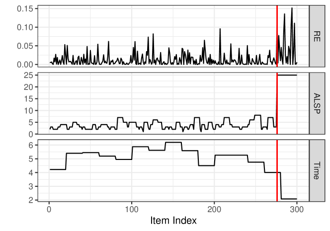
(a) The three dimensions indicative of carelessness. “RE” denotes the autoencoder reconstruction error, “ALSP” is the AdaptiveLongstringPattern sequence, and “Time” the per-page response time.

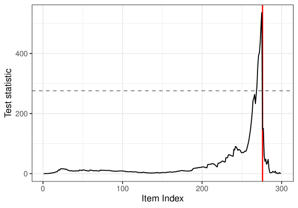
(b) The per-response test statistic of the changepoint detection test. The dashed horizontal line corresponds to the associated critical value at significance level 0.1%.

Figure 2: Illustrative example of the three dimensions indicative of carelessness (top panel) and the associated per-response test statistic (bottom panel) for 300 simulated responses (15 pages comprising 20 items each). In this example, the simulated participant is partially careless, where carelessness onsets at the 276th item (red line) and manifests in content-independent pattern responses such as 1-2-3-1-2-3.

For each participant, we can obtain up to three individual series of length equal to the survey’s total number of items. Each individual series measures one of the three dimensions indicative of carelessness. Specifically, the three dimensions are the reconstruction errors in (1), an AdaptiveLongstringPattern sequence, and response time. It may be preferable to have all three dimensions available for each participant, but our proposed method can also be applied to single dimensions or two dimensions, for instance when response times cannot be measured. For now, we assume that all three dimensions can be measured and are collected in a three-dimensional series.

As motivated in the previous two sections, we expect changepoints in each dimension from the onset of careless responding (e.g., Figure 2(a)), and no changepoint in the absence of carelessness. Therefore, we propose to use a statistical method designed for the detection of a single changepoint in a multidimensional series. Concretely, we propose to use the nonparametric cumulative sum self-normalization test of Shao & Zhang, (2010), which searches for the location of a possible changepoint in a multivariate series and derives a corresponding statistical test. This test has attractive theoretical guarantees that are derived in Shao & Zhang, (2010) and Zhao et al., (2021).

The changepoint detection method of Shao & Zhang, (2010) calculates the value of a certain test statistic for each multidimensional element in a given series. If the maximum value of the test statistic exceeds a specific critical value, the method flags a changepoint located at the associated element. If the critical value is never exceeded, no changepoint is flagged. The the critical value is implied by the choice of the significance level of the test. Following Huang et al., (2012), we recommend an extraordinarily low significance level of 0.1% so that the test becomes extremely conservative in flagging changepoints. Our extremely conservative approach is consonant with the literature, as there should be overwhelming evidence in favor of careless responding when labeling respondents as such (cf. Huang et al.,, 2012).

We provide a detailed description of the method of Shao & Zhang, (2010) in Appendix C.2. In practice, we apply this method to each participant’s individual three-dimensional series to locate the onset of carelessness (or an absence thereof) for each participant. As an example, Figure 2(b) shows a series of per-response test statistics associated with a three-dimensional series in Figure 2(a), and the corresponding (simulated) respondent becomes careless after the 276th of 300 items (content-independent pattern responding). Indeed, the maximum test statistic occurs at the 276th item and the maximum value exceeds the critical value at significance level 0.1% so the test flags a changepoint at this item.

4 Simulation Experiments

4.1 Data Generation

We demonstrate our proposed method on simulated data inspired by existing survey measures and empirical findings on careless responding. For this purpose, we generate rating-scale responses of $n=500$ respondents to $p=300$ items using the simstudy package (Goldfeld & Wujciak-Jens,, 2020). Each item has five Likert-type answer categories (anchored by 1 = “strongly disagree” and 5 = “strongly agree”) whose probability distribution can be found in Table 1. The $p=300$ items comprise 15 constructs, each of which are measured through 20 items (of which 10 are reverse-worded), resulting in the aforementioned $15\times 20=300$ items. We assume that there are 15 pages of 20 items each and that each participant is presented with the same randomly ordered set of $p=300$ items. We simulate construct reliability by imposing that items from different constructs are mutually independent and items within a construct have a correlation coefficient of $\pm 0.7$. Each construct has a Cronbach-$\alpha$ value of 0.979 on the population level and is therefore highly reliable in the absence of carelessness.

$\mathbb{P}[X=1]$	$\mathbb{P}[X=2]$	$\mathbb{P}[X=3]$	$\mathbb{P}[X=4]$	$\mathbb{P}[X=5]$
0.05	0.25	0.40	0.25	0.05

Table 1: Probability distribution of a given response, $X$, with five answer categories.

We simulate per-item response times (in seconds) of attentive respondents as draws from a Weibull distribution with scale and shape parameters equal to six and two, respectively. This results in an expected per-item response time of about 5.3 seconds, which is based on data in Schroeders et al., (2022). The blue line in Figure 3(a) illustrates the distribution of these response times. We then calculate the total time a participant spends on each page of the simulated survey, divided by the number of items on each page, and use the ensuing per-page response times for the response time dimension.

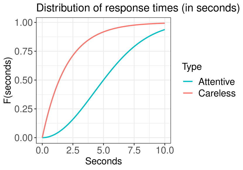
(a) Distribution of per-item response times

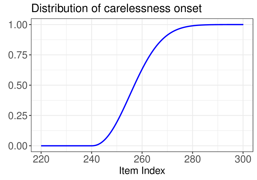
(b) Distribution of carelessness onset items

Figure 3: Weibull distributions of response times (left) and carelessness onset items (right).

Of the $n=500$ respondents, we fix a (relative) prevalence of partially careless respondents of $\gamma\in\{0,0.2,0.4,0.6,0.8,1\}$. For the selected partially careless respondents, we sample carelessness onset items, from which on all responses are careless. We sample onset items as draws—rounded to the nearest integer—from a three-parameter Weibull distribution with location, scale, and shape parameters equal to 240, 20, and 2.2, respectively. We visualize this distribution in Figure 3(b). For instance, this design postulates a probability of about 90% that carelessness onsets before having answered 90% of all items, which reflects estimates in Table 6 in Bowling et al., 2021a for ordinary surveys with 300 items.

We introduce carelessness by replacing with careless responses all responses that come after the sampled carelessness onset item, including the onset item itself. We simulate the following four different types of careless responses that each reflect careless response styles. First, random responding (noncontingent responding in Baumgartner & Steenkamp,, 2001), which is characterized by choosing answer categories completely at random. Second, straightlining, which is characterized by constantly choosing the same, randomly determined answer category. This response style is a special case of aquiescence due to carelessness (see Table 1 in Baumgartner & Steenkamp,, 2001, for details). Third, pattern responding (Schroeders et al.,, 2022), which is characterized by a fixed, randomly determined pattern, such as 1-2-3-1-2-3 or 5-4-5-4. Fourth, extreme responding due to carelessness (Baumgartner & Steenkamp,, 2001), which is characterized by randomly choosing between the two most extreme answer categories, regardless of item content.

In addition to these four careless response styles, we also consider the case of fully attentive responding. This reflects respondents who never becomes careless; we call such respondents attentive. Recall that we consider carelessness prevalence levels $\gamma\in\{0,0.2,\dots,1\}$, which implies that $(1-\gamma)n$ respondents never become careless. In each dataset that includes careless responding, we ensure that all four careless response styles as well as fully attentive respondents are present. To achieve this, we assign to each of the $\gamma n$ partially careless respondents one of the four careless response styles so that there are $\gamma n/4$ partially careless respondents who adhere to that particular response style from their corresponding carelessness onset item onward. We determine at random which respondents are partially careless and which ones are attentive.

Like the given responses, we introduce carelessness to the response times by replacing all per-item response times from the carelessness onset item onward with draws from a Weibull distribution of unit shape and scale equal two; see Figure 3(a). This distribution implies an average careless response time of two seconds per item, which is based on the “two-seconds-per-item” rule of Huang et al., (2012) and Bowling et al., 2021b . We again calculate the per-page response times from the per-item times and use the per-page times for the response time dimension.

We repeat the above described data generating process 100 times. Importantly, we keep the location of carelessness onset of each participant constant across the 100 repetitions. This will be useful for performance assessment. We apply our proposed method to each dataset and report the estimated location of each flagged changepoint.

We search for changepoints in all seven possible combinations of the three dimensions (reconstruction error, AdaptiveLongstringPattern, per-page response time) via the changepoint detection method of Shao & Zhang, (2010). We report the results of the following four cases that are of primary interest: all three dimensions, the two dimensions of reconstruction errors and AdaptiveLongstringPattern sequences that remain when excluding response time (since measuring time may not be feasible in pen-and-paper questionnaires), and the two separate individual dimensions thereof. This separation will help highlight the added value of combining different indicators of carelessness in the hope of capturing different manifestations thereof.

4.2 Performance Measures

We wish to quantify the accuracy of the location of each flagged changepoint. For this purpose, we use the Adjusted Rand Index (ARI; Hubert & Arabie,, 1985). The ARI is a continuous measure of classification performance and takes value 0 for random classification and value 1 for perfect classification. In wake of this, we take the perspective of viewing the detection of carelessness onset as classification problem: For each item, a simulated respondent either responds attentively or carelessly. Using the true location of changepoints (the carelessness onset items), the ARI measures how well our method has estimated the location of carelessness onset of a given respondent. Specifically, the closer the ARI is to its maximum value 1, the better our method performs at accurately estimating carelessness onset. ARI values close to 0 indicate poor performance. If the respondent of interest is attentive and there are consequently no careless responses, then the ARI assumes value 0 if a changepoint is flagged. We provide a mathematical definition of the ARI in Appendix C.3.

We average the ARIs of multiple respondents (either all respondents or subgroups thereof) and report the resulting average. Note that when averaging over ARIs calculated on attentive respondents, we obtain the proportion of attentive respondents who are correctly identified as attentive. If we deduct this number from 1, we obtain the proportion of attentive respondents that are incorrectly flagged as careless.

4.3 Results

We start presenting the results of our proposed method for the three dimensions by means of a visual inspection. For a carelessness prevalence level of $\gamma=0.6$, Figure 4 displays a heatmap holding the indices of the participants in its rows and the item indices in its columns. For participant $i\in\{1,\dots,n\}$ and item $j\in\{1,\dots,p\}$, the color scale of the cell at position $(i,j)$ measures the frequency across the 100 repetitions with which the response of participant $i$ to item $j$ has been flagged as changepoint: The darker the red scale, the more frequently the corresponding item was flagged as changepoint. The blue rectangles in Figure 4 visualize the true location of the careless onset items; recall that those are fixed across the repetitions. The $y$-axis of the plot is rearranged so that the participant indices are ordered according to their respective carelessness onset. Since the carelessness onset items stay constant across the repetitions, a good detection performance is characterized by flagging cells that correspond to onset items. Indeed, we can see that there is a dark red band that closely follows the blue rectangles. This means that our method accurately estimated the location of carelessness onset of the participants. Note that the top 40% of the rows in Figure 4 very rarely see flagged changepoints. Those are the respondents who never become careless. Based on this visual example, our method seems to not only accurately estimate the careless onset, but also discriminate well between partially careless respondents and fully attentive respondents. Results are similar for other carelessness prevalence levels, and we provide corresponding heatmaps in Appendix D.1.

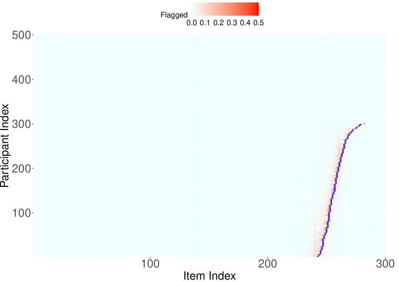
Figure 4: Heatmap visualizing the changepoint detection performance of our proposed method when 60% of all $n$ respondents are partially careless, at significance level 0.1%. The more darker a cell in this heatmap, the more frequently across the 100 repetitions this cell was flagged as carelessness onset item ($x$-axis) of a given respondent ($y$-axis). The blue rectangles denote the true carelessness onset items (which are constant across the repetitions) and the $y$-axis is rearranged according to the location of true carelessness onset. An absence of a blue rectangle (occurs in 40% of all respondents) indicates that a given respondent never becomes careless.

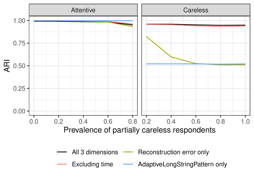
(a) ARI of fully attentive respondents against partially careless respondents.

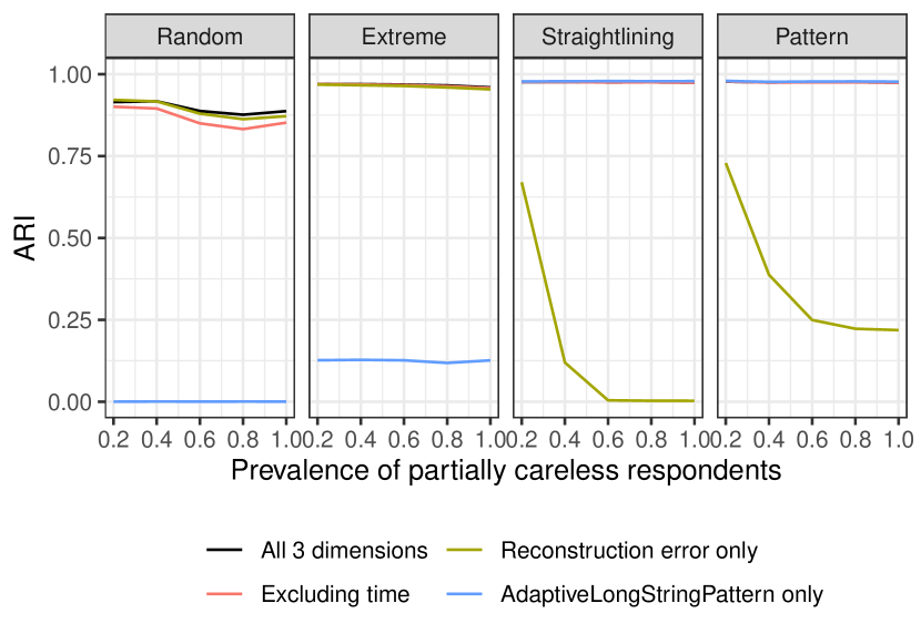
(b) ARI of each careless response style. Note that for extreme respondents, all methods (except AdaptiveLongstringPattern only) perform nearly equally well, resulting in overplotted lines. The same happens in straightliners and pattern respondents for all methods except only reconstruction errors.

Figure 5: ARI estimates for varying carelessness prevalence, averaged over different subgroups.

Varying the prevalence of careless responding, Figure 5(a) visualizes the ARI averaged over all attentive respondents (left panel) and all partially careless respondents (right panel). In the left panel of Figure 5(a), each of the four specifications rarely flag changepoints in fully attentive respondents, even in samples where carelessness is extremely prominent (80% prevalence). For instance, for carelessness prevalence of up to 60%, the proportion of incorrectly flagged changepoints in attentive respondents is less than 0.01. Only when carelessness prevalence is extremely high at 80%, the proportion of false positives slightly increases to about 0.05 for each specification (except AdaptiveLongstringPattern, which remains below 0.01). The right panel in Figure 5(a) visualizes the ARI when averaged over partially careless respondents. The ARI of our proposed method with the three dimensions remains remarkably constant at about 0.95 throughout carelessness prevalence levels, mirroring an excellent performance of flagging changepoints in correct locations. Notably, excluding the time dimension results in only a relatively small decrease in ARI. This may be because in our data generation process, careless response times are faster for all types of careless responses. In contrast, when using solely autoencoder reconstruction errors or AdaptiveLongstringPattern sequences, we observe a drop in ARI values to about 0.5 in high carelessness prevalence levels. This drop in performance is expected due to different careless response styles being present: Reconstruction errors are designed to capture inconsistent carelessness such as random responses and may therefore miss invariant carelessness, while AdaptiveLongstringPattern sequences are designed for capturing invariant carelessness such as straightlining and may therefore miss inconsistent carelessness.

To explore this further, Figure 5(b) displays ARIs for each careless response style. As expected, using reconstruction errors to detect the onset of carelessness works well for inconsistent response styles such as random or extreme responding, resulting in ARI values of about 0.85–0.95 throughout all carelessness prevalence levels, but does not accurately capture invariable response styles (ARIs of less than 0.02). Conversely, using AdaptiveLongstringPattern sequences works well for detecting invariable careless response styles such as straightlining or pattern responding (ARI of consistently about 0.95), but does not work for inconsistent carelessness (ARI of about 0–0.1). However, when combining AdaptiveLongstringPattern and reconstruction errors (and possibly response time), we obtain high ARI values (0.85–0.99) throughout all considered careless response styles. We derive from this that our method succeeds in combining complimentary indicators for carelessness onset to capture different manifestations of careless responding.

4.4 Additional Simulations and Conclusions

We have conducted a wide variety of additional simulation experiments, which are described and discussed in Appendix D.1. They suggest that our proposed method consistently performs well, even in substantially more complex designs, for instance when there is a large degree of response heterogeneity. However, in highly complex designs with overwhelmingly many careless respondents (prevalence of $\geq 80\%$), our method sometimes identifies changepoints in too many attentive respondents (more than a significance level of 0.1% would suggest). Since this issue only arises in specific situations and for extremely high carelessness prevalence, we leave addressing it to further research. Overall, the findings presented in the main text are representative, meaning that they are robust across distinct simulation designs.

We conclude from our simulation experiments that our proposed method seems to perform well for reliably detecting carelessness onset, while simultaneously successfully discriminating between partially careless respondents and fully attentive respondents. In addition, our simulations highlight the importance of using multiple indicators to capture different manifestations of carelessness (cf. Goldammer et al.,, 2020; Huang et al.,, 2012; Meade & Craig,, 2012; Ward & Meade,, 2022).

5 Empirical Validation

A major challenge in the empirical validation of our method is that the onset of potential carelessness is unknown in empirical data, but such knowledge is required to evaluate the accuracy of our method in locating carelessness onset (or a lack thereof). We therefore employ the following validation strategy. We use a rich empirical dataset of high quality, in the sense that all scales are reliably measured and careless responding is absent. Such a dataset allows us to artificially introduce partially careless responses by replacing given responses with simulated careless ones. In the ensuing hybrid dataset, we can evaluate the performance of our method in a realistic data configuration, as opposed to the stylized data configuration from the simulations.

For empirical validation, we consider empirical data for the five factor model of personality (Costa & McCrae,, 1992; Goldberg,, 1992). This model assumes that variation in a measurement of personality can be explained by the five personality traits (“factors”) of neuroticism, extraversion, agreeableness, openness, and conscientiousness, which are commonly referred to as the “Big 5”. A popular way of measuring the Big 5 is the NEO-PI-R instrument of Costa & McCrae, (1992), which comprises 240 items that collectively measure six subdomains (“facets”) for each of the Big 5 factors (e.g., depression and anxiety are facets of the neuroticism trait), resulting in a measurement of $5\times 6=30$ facets. Each facet is measured with eight items, each of which is answered on a five-point Likert scale. Overall, this instrument measures 30 constructs (the facets).

We use a dataset of Dolan et al., (2009), who administered a Dutch translation of the NEO-PI-R instrument (Hoekstra et al.,, 2003) to 500 first year psychology students at the University of Amsterdam in The Netherlands. The items of the instruments were presented in a random, but identical order to all participants and the dataset is publicly available in the R package qgraph (Epskamp et al.,, 2012). Unfortunately, the data only contain the students’ responses, but no response times, so we restrict our analysis of careless responding to the two dimensions of autoencoder reconstruction errors and AdaptiveLongstringPattern sequences. In addition, we do not have information on the page membership of each item, hence we do not include such information in the autoencoder architecture. Moreover, 175 of the $500\times 240=120,000$ total responses are not contained in the set of admissible answer categories $\{1,2,3,4,5\}$ implied by five-point Likert scales, for instance values such as 3.31 or 4.03. Such inadmissible values may be due to prior imputation of missing responses or other data preprocessing. However, since there is no information on what kind of preprocessing was performed for those observations, we drop all students that have at least one inadmissible response, resulting in a final sample of $n=400$ students.

In general, the dataset of Dolan et al., (2009) as provided by Epskamp et al., (2012) seems to be of high quality as it appears to be carefully cleaned and preprocessed, all five factors are measured very reliably (indicated by Cronbach-$\alpha$ estimates of 0.92, 0.88, 0.85, 0.88, and 0.90 for neuroticism, extraversion, openness, agreeableness, and conscientiousness, respectively), and factor loadings align well with theory (Dolan et al.,, 2009; Epskamp et al.,, 2012). We consequently do not expect careless responding to be an issue in this dataset. Indeed, when applying our proposed method, a changepoint is only flagged in one of the 400 participants at a significance level of 0.1% (see Appendix D.2 for details).

For empirical validation, we take a fixed number of students and from a certain item onward replace their given responses by synthetically generated careless responses. This results in a dataset comprising empirical attentive responses and synthetic careless responses. On this hybrid dataset, we can empirically validate our method since we have knowledge of the true onsets of careless responding. Concretely, of the $n=400$ students in the data of Dolan et al., (2009), we fix the prevalence of to-be partially careless respondents to $\gamma\in\{0.2,0.4,0.6,0.8,1\}$ and sample a carelessness onset item for each partially careless respondent. We replace the given responses from the onset item onward by synthetically generated careless responses. For each to-be careless respondent, we randomly sample the onset item to be between the 160th and 204th item, which respectively correspond to $66.7\%$ and $85\%$ of the 240 items. Like in the simulation setup of Section 4, we again consider the four careless response styles of random, extreme, pattern, and straightlining responding, each of which are set to be present in $\gamma n/4$ of all students. We again calculate the Adjusted Rand Index (ARI) of each student and average across the $n$ students. We repeat this procedure 100 times, where we sample anew in each replication the to-be careless students, carelessness onsets, and careless respondents. We report the ARI averages across the repetitions.

(a) ARI of attentive and careless respondents.
 
 

(b) ARI of each careless response style. Note that the ARIs of straightliners and pattern respondents are nearly identical, resulting in overplotted lines.

Figure 6: ARI estimates for varying carelessness prevalence, averaged over different subgroups at significance level 0.1%, using the hybrid data based on the NEO-PI-R administration of Dolan et al., (2009). We used the two-dimensional series comprising autoencoder reconstruction errors and AdaptiveLongstringPatternsequences.

Figure 6 visualizes the results at significance level 0.1%. Just like in the simulation experiments, almost no attentive respondents are incorrectly identified as careless. Conversely, for the careless respondents, using both dimensions of autoencoder reconstruction errors and AdaptiveLongstringPattern results in ARI values of about 0.8 across all considered carelessness prevalence levels. Plotting ARIs by careless response styles reveals that onsets of straightlining or pattern carelessness are very accurately estimated when using both dimensions, with ARI values of more than 0.95. Likewise, the ARIs of careless extreme responding are consistently at about 0.85. The ARIs for random careless responding amount to about 0.4–0.45. A quick inspection reveals that they are due about half of the random respondents not being identified as careless (i.e., no changepoints), which may be due to the extremely conservative significance level. Indeed, increasing the significance level to 0.5% elevates the ARIs of random respondents to about 0.6 without significantly increasing the number of attentive respondents being incorrectly identified as careless. Further improvements are possible by slightly increasing the significance levels (see Appendix D.2). However, the overall performance across all careless response styles is excellent with an ARI of about 0.8, and almost no attentive respondents are incorrectly identified as careless.

We conclude that our proposed method performs very well on empirical data. Nevertheless, at extremely conservative significance levels, some random respondents may not be identified as careless. While this smaller drawback can be alleviated by choosing significance levels to be slightly less conservative (such as 0.5%), we still recommend to follow the literature by requiring overwhelming evidence in favor of carelessness to label respondents as (partially) careless (cf. Huang et al.,, 2012), and therefore maintain our suggestion to opt for a significance level of 0.1%.

6 Alternatives and Limitations

In this section, we discuss potential alternatives to our proposed method and its limitations.

6.1 Potential Alternatives to Our Method

In general, one may argue that the onset of carelessness can be detected by a priori including detection items in the survey: A survey designer may follow a recommendation of Meade & Craig, (2012) and include at most three bogus, instructed, or self-report items and space them every 50–100 items. One may treat it as evidence of the onset of carelessness if a participant fails a detection item by not providing the response that would be expected from an attentive respondent. However, there are a number of practical and theoretical disadvantages with this approach. First, the recommendation that one should not include more than three detection items (Meade & Craig,, 2012) is fairly restrictive as carelessness may have onset at a much earlier item than the detection item, resulting in a failure to exclude a potentially large number of careless responses. Second, attentive respondents may ironically choose a “wrong” response to a bogus item because they find doing so humorous (Meade & Craig,, 2012) or they misinterpret the item (Curran & Hauser,, 2019). Third, a careless respondent may choose the “correct” response by mere chance or lie in self-report items (DeSimone & Harms,, 2018; Edwards,, 2019), resulting in overlooking this careless respondent. Fourth, it is unclear if a “somewhat disagree” response to a detection item to which “strongly disagree” is expected should be considered careless (Ward & Meade,, 2022). Fifth, it may not be possible to include detection items in the survey for legal or ethical reasons, or the survey analyst has no control over the survey design.

Moreover, the R packages careless (Yentes & Wilhelm,, 2021) and ufs (Peters & Gruijters,, 2021) support the calculation of an intra-individual variance (IRV) across subsets of responses. If sets of responses towards the end of a survey exhibit a sufficiently larger (Marjanovic et al.,, 2015) or lower (Dunn et al.,, 2018) variance than earlier sets of responses, there might evidence for an onset of partially careless responding. However, it would require the user to a priori know in which subsets of responses carelessness occurs in order to confirm the presence of partial carelessness in these subsets. In addition, it is unclear when a variance can be considered sufficiently low or high to infer carelessness: Determining cutoff values below or above which a participant is to be flagged as careless may depend on survey design and survey content.

Instead of detecting careless responding, one may attempt to prevent such behavior during survey administration. Preventive measures against careless responding may entail promising rewards for responding accurately (Gibson & Bowling,, 2020), threatening with punishment for careless responding, and the presence of a proctor (Bowling et al., 2021a, ). There is evidence that each of these three preventive measures can prevent or at least delay carelessness onset (Bowling et al., 2021a, ; Gibson & Bowling,, 2020; Huang et al.,, 2012). However, either of these three preventive measures can be undesirable or unethical in practice: Administering proctored questionnaires is often impractical and expensive, and is typically infeasible in online studies. Arthur et al., (2021) and Bowling et al., 2021a advise against using threats if one wishes to maintain a positive long-term relationship with questionnaire participants, such as when there is a professional relationship between researcher and participants. In addition, threats seem inappropriate in longitudinal studies or when the participants are members of a questionnaire panel (as is common in survey research) or when they are suspected to suffer from anxiety, trauma, or depression (as is common in psychological research). On the other hand, promising rewards may cross ethical boundaries in organizational surveys and in the context of employment-related decisions (Arthur et al.,, 2021).

Notwithstanding, we stress that preventive methods against carelessness are complementary to detection methods (such as ours) for the overarching goal of improving the reliability of collected questionnaire data. If possible and ethical, we recommend that survey designers take preventive measures against careless responding, include detection items, and—after questionnaire administration—analyze the data for the presence of careless responding through detection methods. As a result, one minimizes the probability that the analyzed data are plagued by (undetected) careless responding, thereby enhancing data quality and reliability.

6.2 Limitations

Throughout this paper, we have assumed that all participants start as truthful and accurate respondents, while some of them may begin to respond carelessly from a certain item onward. However, in certain scenarios, this assumption may not hold true. In the following, we discuss two such scenarios.

First, there may be some participants who alternate between periods of accurate and careless responding (Berry et al.,, 1992; Clark et al.,, 2003; Meade & Craig,, 2012). In this case, our method may only flag one of the possibly multiple changepoints. Extending our method to this situation is an area of further research.

Second, some respondents may respond carelessly throughout all survey items. Consequently, our method is unlikely to flag a changepoint since there is no change in behavior. This is clearly undesirable because we would like to identify all participants who have engaged in careless responding. Nevertheless, there is a plethora of established methods for detecting respondents who have been careless throughout the survey (see Section 2). In this sense, our method—which is intended for detecting partial carelessness—is complementary to existing methods that are intended for detecting respondents that have been careless throughout all items. Consequently, if one suspects that respondents who have been careless throughout all items are present, we recommend to apply established detection methods following the guidelines of Arthur et al., (2021) and Ward & Meade, (2022). Participants which are flagged as careless by these methods, but for which no changepoint was flagged by our method have likely been careless throughout the entire survey.

Response time is one of the three dimensions along which our proposed method may search for changepoints. However, in some series of response times, it is possible that there could be “natural” structural breaks due to survey design: For instance, items that naturally take longer to respond to due to higher complexity or length might be placed in the beginning or end of a questionnaire. If the structural break is very pronounced, it may happen that our method identifies a changepoint at this break despite an evidence of carelessness in other dimensions. Studying this issue is left to further research.

Moreover, the changepoint detection procedure of Shao & Zhang, (2010) is based on asymptotic arguments when the number of items is large, hence our method is designed for lengthy questionnaires. It is likely that the statistical power to identify carelessness onset drops considerably in short questionnaires, but studying this is beyond the scope of this paper. However, partial careless responding due to fatigue may be less prevalent in short questionnaires (cf. Bowling et al., 2021a, ).

7 Computational Details

Throughout this paper, we have followed recent guidelines by Alfons & Welz, (2022) on the application of machine learning methods for the detection of careless responding. In particular, an implementation of our proposed method is publicly available from https://github.com/mwelz/carelessonset. We will develop this code into an R package to be submitted to the Comprehensive R Archive Network (https://cran.r-project.org/).

8 Discussion and Future Research

In this paper, we have proposed a method to identify the onset of careless responding (or absence thereof) for each participant in a given survey. Our method is based on recent literature stressing that in lengthy surveys—which are common in the behavioral and organizational sciences—a large proportion of survey participants may respond partially carelessly due to fatigue or boredom. Our method combines three indicators for the potential onset of carelessness and simulation experiments highlight the importance of evidence from multiple indicators that capture different manifestations of carelessness for obtaining reliable estimates for the onset.

Due to our method’s promising performance on empirical and synthetic data, we consider it a promising first step for research on partially careless responding. For instance, the AdaptiveLongstringPattern algorithm may need additional validation as a measurement of response invariability, which could be done in empirical follow-up work. Moreover, Arthur et al., (2021) envisage “artificial intelligence and machine learning being used to detect careless responding and response distortion in real time in the foreseeable future.” We believe that it is possible to train our autoencoder on responses from many different surveys so that it does not need to be re-fitted on every survey. With such a trained autoencoder, we could build reconstruction errors in real time and use them together with live measurements of response time and AdaptiveLongstringPattern to detect the onset of careless responding in real time. Nevertheless, detecting changepoints in real time may require the use of a different changepoint detection method that is designed to detect changepoints as soon as they happen. Such methods are called online changepoint detection methods; an overview of which is provided in Li et al., (2019) and references therein.

Furthermore, De Jong et al., (2008) explicitly model careless responding via Item Response Theory. This approach assumes that careless responding is due to certain characteristics on the participant level. Nevertheless, fatigue in long surveys is likely to be an additional explanatory factor for careless responding (cf. Bowling et al., 2021a, ). We speculate that estimates of the onset of careless responding could be used to extend the model of De Jong et al., (2008) to account for survey fatigue.

Overall, our proposed method could be a starting point for an exciting and fruitful new direction of research on careless responding, in which artificial intelligence and machine learning could play a key role (cf. Alfons & Welz,, 2022).

Appendix A Setup and Assumptions

Throughout our paper, we consider the following setup. Let $\bm{X}$ be an $n\times p$ data matrix holding the rating-scale survey responses of $n$ respondents to $p$ items. We assume that all observations (i.e. all respondents whose responses the survey collects) are independently and identically distributed, which is a standard assumption in statistics and machine learning. Moreover, we do not know if and when careless responding occurs in $\bm{X}$. We require four more assumptions, which are listed below.

Assumption 1.

The responses in $\bm{X}$ admit an $n\times s$ lower-dimensional representation, $\bm{S}$, where $s\ll p$. The dimension $s$ is known and corresponds to the number of constructs the survey measures.

Assumption 2.

The survey that generated $\bm{X}$ is reliable in the sense that if all participants responded accurately, $\bm{X}$ would accurately measure all constructs.

Assumption 3.

All participants begin the survey as attentive respondents by providing accurate and truthful responses. As the survey progresses, some (possibly none or all) participants start responding carelessly and continue to do so for the remainder of the survey.

Assumption 4.

The onset of partial carelessness is characterized by a changepoint in either one, two, or all three of the following indicators: autoencoder reconstruction errors (1), AdaptiveLongstringPattern sequences, and response times.

Assumption 1 is very mild in survey data because surveys typically measure multiple constructs and the number of constructs is typically known. We refer to Section 3.1 for a detailed discussion. In the example of the NEO-PI-R instrument (Costa & McCrae,, 1992), there are $p=240$ items that measure $s=30$ constructs.

Assumption 2 is also mild in survey data. There exist well-established and reliable survey measures for a large variety of variables. For instance, the International Personality Item Pool (IPIP; Goldberg,, 1999) is a pool of more than 250 personality scales. It is in general recommended to use well-established measures to ensure a highly reliable measurement (Babbie,, 2020, p. 150). The reliability of a measurement can be estimated in multiple ways, such as Cronbach’s alpha, the omega coefficient and variations thereof, as well as the $H$ coefficient; we refer to McNeish, (2018) for a description of these and other reliability measures. Hence, Assumption 2 is satisfied when the survey data were collected with measures of high reliability,

Assumption 3 is discussed in Section 6.2 and Assumption 4 is motivated in detail in Section 3.

Appendix B Details of Autoencoders

B.1 Network Architecture and Estimation

Denote by $x_{ij}$ the response of the $i$-th participant to the $j$-th survey item. Collect the responses of the $i$-th participant to all $p$ items in a $p$-dimensional vector $\mathbf{x}_{i}=(x_{i1},x_{i2},\dots,x_{ip})^{\top}$. Hence, the $n\times p$ data matrix $\bm{X}$ is given by $\bm{X}=(\mathbf{x}_{1},\mathbf{x}_{2},\dots,\mathbf{x}_{n})^{\top}$.

An autoencoder is a network with the following architecture. The network consists of $M$ layers, where the first layer holds the input data $\mathbf{x}_{i}$ (input layer) and the last layer (output layer) holds the reconstructed input data. Let the $\ell$-th layer contain $N^{(\ell)}$ nodes. Since the first layer is the input layer, the last layer is the output layer, and an autoencoder attempts to reconstruct its input variables, we have that $N^{(1)}=N^{(M)}=p$.

Each node in a given layer contains an activation, which is a function of transformed activations from previous layers. Transformations in the $\ell$-th layer are obtained through what is called an activation function $g_{\ell}(\cdot)$. Formally, for participant $i=1,\dots,n$, the activation $a_{ij}^{(\ell)}$ of the $j$-th node, $j=1,\dots,N^{(\ell)},$ of the $\ell$-th layer, $\ell=2,\dots,M$, is given by

$$a_{ij}^{(\ell)} =g_{\ell}\left(z_{ij}^{(\ell)}\right),\qquad\text{where}$$

$$z_{ij}^{(\ell)} =\sum_{k=1}^{N^{(\ell-1)}}\omega_{jk}^{(\ell)}a_{ik}^{(\ell-1)}+b_{j}^{(\ell)}.$$

The $\omega_{jk}^{(\ell)}$ are fixed but unknown weights and the $b_{j}^{(\ell)}$ are intercept terms, which are also fixed and unknown. Observe that in the first layer, we have $a_{ij}^{(1)}=x_{ij}$. The activations of the last layer, $a_{ij}^{(M)}$, hold the network’s output, which correspond to the autoencoder’s reconstruction of responses $x_{ij}$.

We jointly refer to the weights and intercept terms as the network’s parameters. Since the parameters are unknown in practice, they need to be estimated. We collect in a vector $\bm{\theta}$ all parameters that need to be estimated. To emphasize the dependence on the parameter vector $\bm{\theta}$, we define for a fixed $\bm{\theta}$ a prediction function $\bm{f}_{\bm{\theta}}(\cdot)$ of the network, which corresponds to the activations in the last layer:

$$\bm{f}_{\bm{\theta}}(\mathbf{x}_{i})=\Big{(}f_{1,\bm{\theta}}(\mathbf{x}_{i}),f_{2,\bm{\theta}}(\mathbf{x}_{i}),\dots,f_{p,\bm{\theta}}(\mathbf{x}_{i})\Big{)}^{\top}=\left(a_{i1}^{(M)},a_{i2}^{(M)},\dots,a_{ip}^{(M)}\right)^{\top},$$

for participants $i=1,\dots,n$. The reconstruction of the input vector $\mathbf{x}_{i}$ is then given by $\widehat{\mathbf{x}}_{i}~{}=~{}\bm{f}_{\bm{\theta}}(\mathbf{x}_{i})$.

Because of the fact that each node is a function of nodes from a previous layer, the nodes in adjacent layers are often visualized by connecting edges. For instance, Figure B.1 provides a schematic overview of an autoencoder neural network.

Figure B.1: Schematic example of an autoencoder neural network with $M$ layers. The first and last layer are referred to as input and output layer, respectively. For participants $i=1,\dots,n$, the input in the first layer are the input responses, $\mathbf{x}_{i}=(x_{1},\dots,x_{p})^{\top}$ and the output in the last layer are the activations $f_{j,\bm{\theta}}(\mathbf{x}_{i})=a_{ij}^{(M)},\ j=1,\dots,p,$ that reconstruct the input responses for a fixed parameter vector $\bm{\theta}$. The $j$-th node in the $\ell$-th layer holds the activation $a_{ij}^{(\ell)}$, for $\ell=2,\dots,M,j=1,\dots,N^{(\ell)}$. Besides the parameter vector $\bm{\theta}$, the prediction function $\bm{f}_{\bm{\theta}}(\cdot)$ depends implicitly on the prespecified choice of the activation functions $g_{\ell}(\cdot)$.

To fit an autoencoder, we aim at minimizing its reconstruction error. For a prespecified loss function $\mathcal{L}(\cdot)$, we fit the neural network by finding the $\bm{\theta}$ that yields the best average reconstruction error,

$$\widehat{\bm{\theta}}=\arg\min_{\bm{\theta}}\Bigg{\{}\frac{1}{n}\sum_{i=1}^{n}\sum_{j=1}^{p}\mathcal{L}\Big{(}x_{ij}-f_{j,\bm{\theta}}(\mathbf{x}_{i})\Big{)}\Bigg{\}}.$$ (B.1)

The prediction function of the fitted network is subsequently given by $\bm{f}_{\widehat{\bm{\theta}}}(\cdot)$. For the loss function in (B.1), we choose the smooth and robust Pseudo-Huber loss, which is defined for a fixed $\delta>0$ as

$$\mathcal{L}(z)=\delta^{2}\left(\sqrt{1+(z/\delta)^{2}}-1\right).$$ (B.2)

This choice results in quadratic loss for small values of $z$ and linear loss for large values of $z$. Consequently, the Pseudo-Huber loss function avoids that large individual reconstruction errors strongly affect the fit, which would make it hard for the network to distinguish ordinary observations from irregular observations, as the latter typically lead to large prediction errors. To solve the optimization problem in (B.1), we use stochastic gradient descent. We refer to Chapter 8.5 in Goodfellow et al., (2016) for details.

The optimization problem (B.1) can be generalized by adding a penalty term $\lambda\Omega(\cdot)$ to the optimization criterion, where $\lambda\geq 0$ is a prespecified tuning parameter. The penalized version of (B.1) reads

$$\widehat{\bm{\theta}}\in\arg\min_{\bm{\theta}}\Bigg{\{}\frac{1}{n}\sum_{i=1}^{n}\sum_{j=1}^{p}\mathcal{L}\big{(}x_{ij}-f_{j,\bm{\theta}}(\mathbf{x}_{i})\big{)}+\lambda\Omega(\bm{\theta}_{\omega})\Bigg{\}},$$ (B.3)

where we use the following definition for a $q$-dimensional parameter $\bm{\theta}_{\omega}$:

$$\bm{\theta}_{\omega}=(\theta_{1\omega},\dots\theta_{q\omega})^{\top},$$

whose components are given by, for $j=1,\dots,q$,

$$\theta_{j\omega}=\begin{cases}\theta_{j}\quad\text{ if $j$-th parameter is a weight parameter},\\ 0\ \quad\text{ if $j$-th parameter is an intercept parameter.}\end{cases}$$

Observe that we only penalize weight parameters, but not intercept parameters. For the penalty function $\Omega(\cdot)$, we choose the group-lasso penalty, which is defined as follows. Let $\{G_{j}\}_{j=1}^{m}$ be a disjoint and exhaustive partition of parameters $\{1,\dots,q\}$ into $m$ groups, that is,

$$G_{j}\subseteq\{1,\dots,q\}\quad\text{for all }j=1,\dots,m,$$

such that $\bigcup_{j=1}^{m}G_{j}=\{1,\dots,q\}$ and $\bigcap_{j=1}^{m}G_{j}=\varnothing.$ The group-lasso penalty is given by

$$\Omega(\bm{\theta}_{\omega})=\sum_{j=1}^{m}\sqrt{\#G_{j}}\sqrt{\sum_{k\in G_{j}}\theta_{k\omega}^{2}},$$ (B.4)

where $\#A$ denotes the cardinality of some set $A$. All parameters in a given group $G_{j}$ are either jointly shrunk to zero or are jointly nonzero (Scardapane et al.,, 2017; Yuan & Lin,, 2006). In our context, each group $G_{j}$ holds items on the same survey page such that the number of groups, $m$, corresponds to the number of survey pages. We apply the group-lasso penalty between the input layer and the mapping layer, which is supposed to let items from later pages (where careless responding is more likely) be routed through different nodes in the mapping layer than items from earlier pages. Figure B.2 provides a schematic example.

Figure B.2: Schematic example of the group-lasso penalty applied to autoencoders in the context of careless responding. This figure uses the same notation as Figure 1. Here, we assume that the first two items (responses $x_{1}$ and $x_{2}$) are on the same page and that the last two items (responses $x_{3}$ and $x_{4}$) are also on the on the same page. The magenta-colored arrows indicate connections associated with the first page, while the blue arrows indicate connections associated with the second page.

B.2 Modeling Choices

Following Kramer, (1992), we specify five layers, $M=5$, and a symmetric network architecture. That is, the number of nodes in input and output layer are equal and correspond to the number of items, $p$. In addition, the number of nodes and types of activation function are equal in the mapping an de-mapping layer (layers 2 and 4, respectively). Specifically, we set the number of nodes in both layers to $\lfloor 1.5\times p\rfloor$ because a relatively large number of nodes is expected to give the autoencoder flexibility to learn many different types of response behavior (attentive and careless). Based on Assumption 1, the number of nodes in the central bottleneck layer equals the number of scales in the questionnaire.

Concerning the activation functions, we again follow a recommendation in Kramer, (1992) and propose to use nonlinear activation functions in the mapping as well as de-mapping layers, and a linear activation function in the bottleneck layer. Specifically, we propose to use the hyperbolic tangent activation in the (de-)mapping layers and the identity mapping in the bottleneck layer. Definitions are given in Table B.1, which summarizes our proposed autoencoder architecture.

Layer	# Nodes	Activation function
Mapping layer	$\lfloor 1.5\times p\rfloor$	$\textsf{tanh}(x)=2/(1+\exp(-2x))-1$
Bottleneck layer	$s$	$\textsf{identity}(x)=x$
De-mapping layer	$\lfloor 1.5\times p\rfloor$	$\textsf{tanh}(x)=2/(1+\exp(-2x))-1$

Table B.1: Network architecture of our autoencoder. The constants $p$ and $s$ denote respectively the number of items in the dataset and the number of scales that the dataset measures. For a real number $x$, the operator $\lfloor x\rfloor$ denotes that largest integer smaller than or equal to $x$.

For fitting the autoencoder, we use the stochastic gradient descent algorithm with a batch size of 10, a learning rate of 0.0001, and 100 epochs. In the presudo-Huber loss (B.2), we set constant $\delta=1$. We set the tuning parameter in the penalized loss function (B.3) to $\lambda=0.01$.

Appendix C Algorithms and Changepoint Detection

C.1 Longstring Pattern Algorithms

In Section 3, we have motivated and described algorithms to compute LongstringPattern and AdaptiveLongstringPattern sequences. Formal algorithms are provided in Algorithms 1 and 2, respectively.

Input: Series of observed rating-scale responses $\{x_{j}\}_{j=1}^{p}$, number of items an individual pattern encompasses $J\in\mathbb{N}$ (pattern length). For instance, the individual pattern 1-2-3 encompasses $J=3$ items in the response sequence 1-2-3-1-2-3. Note that choosing $J=1$ makes the algorithm measure straightlining.

Output: Set of longstring pattern measures $\{LS_{j}\}_{j=1}^{p}$

Initialization: $streak\leftarrow 1,startindex\leftarrow 1$ (algorithm assumes one-indexing)

1

/* fill in the first $J-1$ indices */

2 for $k\leftarrow 1$ to $p-J-1$ by $1$ do

3       if $x[k]==x[k+J]$ then

            increment $streak$ by 1 ;

             // streak is ongoing

4            

5      else

             Assign value $streak$ to all elements in $\{LS_{j}\}_{j=startindex}^{k}$ ;

             // streak just broke

6             $startindex\leftarrow k+1$;

7             streak $\leftarrow 1$;

8            

9       end if

10      

11 end for

12

/* fill in the last $J$ indices (there are 3 edge cases) */

13 if $\texttt{streak}\geq J$ then

       /* case 1: current streak is ongoing and we have seen it completely at least once, so assume it will last until the end and complete the current streak (which has not yet been broken) */

14       Assign value $streak+J-1$ to all elements in $\{LS_{j}\}_{j=startindex}^{p}$;

15      

16 else if $1<\texttt{streak}<J$ then

       /* case 2: there is an ongoing streak, but we have no chance of seeing it completely (since streak < J), so we do not know how the streak looks like. In this case, fill in the current value of "streak" until the (p-J)-th item and fill in 1 for the last J items (because we do not know how the complete streak looks like */

17       Assign value $streak-1$ to all elements in $\{LS_{j}\}_{j=startindex}^{p-J}$;

18       Assign value $1$ to all elements in $\{LS_{j}\}_{j=p-J+1}^{p}$;

19      

20 else

       /* case 3: there is no ongoing streak, so fill in 1 for last $J$ indices */

21       Assign value 1 to all elements in $\{LS_{j}\}_{j=p-J+1}^{p}$;

22      

23 end if

Algorithm 1 LongstringPattern($\{x_{j}\}_{j=1}^{p},J$)

Input: Series of observed rating-scale responses $\{x_{j}\}_{j=1}^{p}$, maximum pattern length $J_{max}\in\mathbb{N}$ to consider

Output: Set of adaptive longstring pattern measures $\{LS_{j}\}_{j=1}^{p}$

1

/* calculate LongstringPattern for fixed pattern length $J$ */

2 for $J\leftarrow 1$ to $J_{max}$ by $1$ do

3       $\{LS^{J}_{j}\}_{j=1}^{p}\leftarrow\texttt{LongstringPattern}(\{x_{j}\}_{j=1}^{p},J)$;

4      

5 end for

6

/* for each element $\{1,\dots,p\}$, report the largest LongstringPattern value */

7 Initialize $\{LS_{j}\}_{j=1}^{p}$;

8 for $j\leftarrow 1$ to $p$ by $1$ do

9       $LS_{j}\leftarrow\max\big{\{}LS_{j}^{1},LS_{j}^{2},\dots,LS_{j}^{J}\big{\}}$;

10      

11 end for

Algorithm 2 AdaptiveLongstringPattern($\{x_{j}\}_{j=1}^{p},J_{max}$)

C.2 Details on Changepoint Detection

In the following, we describe the cumulative sum self-normalization test of Shao & Zhang, (2010), which tests for the presence and location of a single changepoint in a multivariate series.

Let $\{\bm{Y}_{j}\}_{j=1}^{p}$ be a series of length $p$ consisting of $d$-dimensional random variables $\bm{Y}_{j}$. Our goal is to estimate the location of a possible changepoint in the value of this series. Define by $\widehat{\bm{\theta}}_{a,b}=(b-a+1)^{-1}\sum_{j=a}^{b}\bm{Y}_{j}$ the $d$-dimensional mean of the series calculated on the subset implied by periods $a\leq b$. For location $k\in\{1,2,\dots,p-1\}$, define the test statistic

$$T_{p}(k)=\bm{D}_{p}(k)^{\top}\bm{V}_{p}(k)^{-1}\bm{D}_{p}(k),$$ (C.1)

where

$$\bm{D}_{p}(k) =\frac{k(p-k)}{p^{3/2}}\left(\widehat{\bm{\theta}}_{1,k}-\widehat{\bm{\theta}}_{k+1,p}\right),$$

$$\bm{V}_{p}(k) =\bm{L}_{p}(k)+\bm{R}_{p}(k),$$

which are contained in $\mathbb{R}^{d}$ and $\mathbb{R}^{d\times d}$, respectively, with matrices

$$\bm{L}_{p}(k) =\sum_{i=1}^{k}\frac{i^{2}(k-i)^{2}}{p^{2}k^{2}}\left(\widehat{\bm{\theta}}_{1,i}-\widehat{\bm{\theta}}_{i+1,k}\right)\left(\widehat{\bm{\theta}}_{1,i}-\widehat{\bm{\theta}}_{i+1,k}\right)^{\top},$$

$$\bm{R}_{p}(k) =\sum_{i=k+1}^{p}\frac{(p-i+1)^{2}(i-1-k)^{2}}{p^{2}k^{2}}\left(\widehat{\bm{\theta}}_{i,p}-\widehat{\bm{\theta}}_{k+1,i-1}\right)\left(\widehat{\bm{\theta}}_{i,p}-\widehat{\bm{\theta}}_{k+1,i-1}\right)^{\top},$$

which are both contained in $\mathbb{R}^{d\times d}$.

Consider a prespecified threshold $K_{p}>0$. Based on the test statistic in (C.1), flag the single change-point detection location as

$$\widehat{k}=\begin{cases}\arg\max_{k=1,\dots,p-1}T_{p}(k)\quad&\text{if }\max_{k=1,\dots,p-1}T_{p}(k)>K_{p},\\ \varnothing&\text{otherwise.}\end{cases}$$

Shao & Zhang, (2010) and Zhao et al., (2021) derive theoretical guarantees of this procedure and it turns out that an appropriate choice of $K_{p}$ is directly implied by the desired significance level $\alpha\in(0,0.5)$ and the dimension $d$ of the series. Table 1 in Shao & Zhang, (2010) presents values of $K_{p}$ for common choices of $\alpha$ and certain dimensions $d$, which we present in Table C.1. In our case, we have dimension $d=3$ and level $\alpha=0.001$, so we choose threshold $K_{p}=246.8$.

	Dimension $d$
$\alpha$	1	2	3
0.1	29.6	56.5	81.5
0.05	40.1	73.7	103.6
0.025	52.2	92.2	128.9
0.01	68.6	117.7	160.0
0.005	84.6	135.3	182.9
0.001	121.9	192.5	246.8

Table C.1: Critical values $K_{p}$ at various significance levels $\alpha$ and dimensions $d$, taken from Table 1 in Shao & Zhang, (2010).

It is worth to point out that this test can also test for a changepoint in statistics other than the mean, which was considered here. In addition, it can be extended to test for multiple changepoints. We refer the interested reader to Zhao et al., (2021) for details.

In the context of our paper, we use the test statistics (C.1) to test for changepoints in the three-dimensional series

$$\bm{Y}_{j}=\begin{pmatrix}\textsf{RE}_{j}\\ \textsf{AdaptiveLongstringPattern}_{j}\\ \textsf{RT}_{j}\end{pmatrix},\qquad j=1,\dots,p,$$

where $\textsf{RE}_{j}$ is the reconstruction error (1) of a response to item $j$, $\textsf{AdaptiveLongstringPattern}_{j}$ is the value of the AdaptiveLongstringPattern sequence assigned to this response, and $\textsf{RT}_{j}$ is the response time associated with the response. We obtain such a series for each of the $n$ survey participants and subsequently test each of the $n$ series for changepoints.

As a final technical note, response times when measured on page-level and AdaptiveLongstringPattern sequences may exhibit low variation. Computing their variation over a relatively narrow interval—as required by the test statistics in (C.1)—may result in a singular (and therefore not invertible) variation matrix $\bm{V}_{p}(k)$ such that (C.1) cannot be computed anymore. To avoid this issue, we by default inject Gaussian noise of tiny magnitude to each $\textsf{AdaptiveLongstringPattern}_{j}$ and $\textsf{RT}_{j},\ j=1,\dots,p$. Specifically, we inject draws from a normal distribution with mean zero and variance $0.01\times 0.01$. Doing so results in tiny but nonzero variation, which renders $\bm{V}_{p}(k)$ invertible.

C.3 Details on the Adjusted Rand Index

In the following, we describe how the Adjusted Rand Index (ARI; Hubert & Arabie,, 1985) is calculated for the $p$ responses of a single respondent. The ARI is a continuous measure of classification performance and the respondent either responds attentively or carelessly to each item. Denote by $n_{11}$ the number of careless responses that are correctly identified as careless and by $n_{00}$ the number of attentive responses that are correctly identified as attentive. Conversely, denote by $n_{10}$ the number of careless responses that are incorrectly identified as attentive, and by $n_{01}$ the number of attentive responses that are incorrectly identified as careless. Intuitively, $n_{11}$ and $n_{00}$ measure correct classification, whereas $n_{01}$ and $n_{10}$ measure misclassification. With

$$A =\binom{n_{11}}{2}+\binom{n_{00}}{2}+\binom{n_{10}}{2}+\binom{n_{01}}{2},$$

$$B =\binom{n_{00}+n_{01}}{2}+\binom{n_{10}+n_{11}}{2},$$

$$C =\binom{n_{00}+n_{10}}{2}+\binom{n_{01}+n_{11}}{2},$$

$$D =\binom{p}{2},$$

the ARI for the respondent of interest is given by

$$\textnormal{ARI}=\begin{cases}1&\textnormal{ if $n_{10}=p$ or $n_{01}=p$ or $n_{11}=p$ or $n_{00}=p$},\\ \frac{A-BC/D}{(B+C)/2-BC/D}&\textnormal{ otherwise.}\end{cases}$$

Observe that the ARI assumes value 1 if there is no misclassification, which is the maximum value it can take. Hence, for accurate estimates of the carelessness onset item, the ARI will be close to value 1. For very inaccurate estimates of carelessness onset, the ARI will be close to 0, or sometimes even below that. It is unclear how to interpret negative ARI values, but such values only occur rarely. We refer to Steinley, (2004) for a detailed discussion of the ARI’s properties.

It can be shown that if a changepoint is flagged in an attentive respondent, the ARI takes value 0, and when no changepoint is flagged in an attentive respondent, the ARI takes value 1. Hence, when averaging ARIs of attentive respondents, the ensuing average can be interpreted as the proportion of attentive respondents who are correctly identified as attentive. Conversely, averages of ARIs calculated on partially careless respondents do not have a direct interpretation other than “the higher, the better”.

Appendix D Additional Results

D.1 Simulations

D.1.1 Heatmaps for Different Carelessness Prevalence

In the simulation design of Section 4, Figures D.1–D.4 visualize heatmaps akin to Figure 4 (in which careless prevalence is 60%) for careless prevalence levels of 20%, 40%, 80%, and 100%. All figures use changepoint estimates obtained at significance level 0.1%.

Figure D.1: Heatmap visualizing the changepoint detection performance of our proposed method when 20% of all $n$ respondents are partially careless, at significance level 0.1%. The more darker a cell in this heatmap, the more frequently across the 100 repetitions this cell was flagged as carelessness onset item ($x$-axis) of a given respondent ($y$-axis). The blue rectangles denote the true carelessness onset items (which are constant across the repetitions) and the $y$-axis is rearranged according to the location of true carelessness onset. An absence of a blue rectangle (occurs in 80% of all respondents) indicates that a given respondent never becomes careless.

Figure D.2: Heatmap visualizing the changepoint detection performance of our proposed method when 40% of all $n$ respondents are partially careless, at significance level 0.1%. The more darker a cell in this heatmap, the more frequently across the 100 repetitions this cell was flagged as carelessness onset item ($x$-axis) of a given respondent ($y$-axis). The blue rectangles denote the true carelessness onset items (which are constant across the repetitions) and the $y$-axis is rearranged according to the location of true carelessness onset. An absence of a blue rectangle (occurs in 60% of all respondents) indicates that a given respondent never becomes careless.

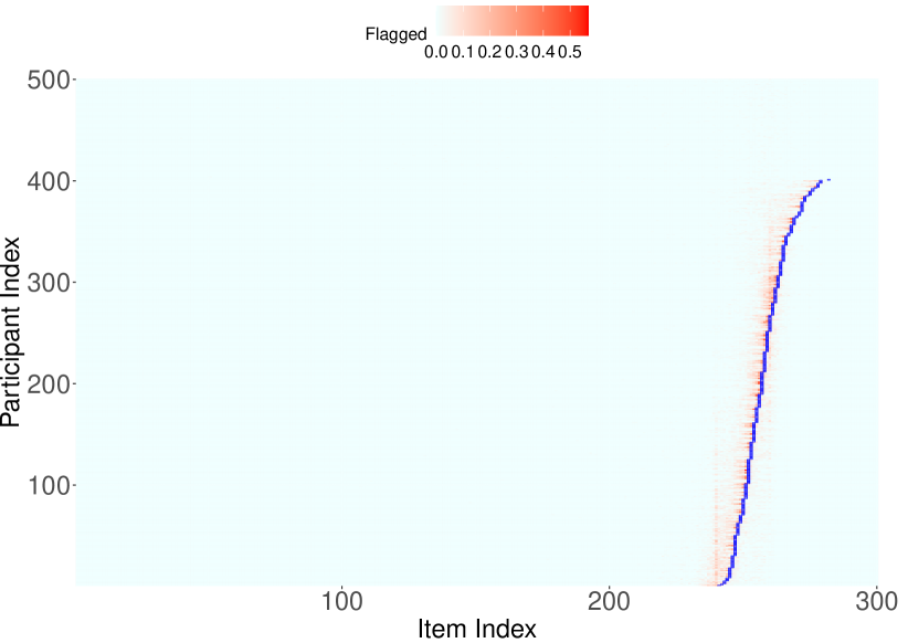
Figure D.3: Heatmap visualizing the changepoint detection performance of our proposed method when 80% of all $n$ respondents are partially careless, at significance level 0.1%. The more darker a cell in this heatmap, the more frequently across the 100 repetitions this cell was flagged as carelessness onset item ($x$-axis) of a given respondent ($y$-axis). The blue rectangles denote the true carelessness onset items (which are constant across the repetitions) and the $y$-axis is rearranged according to the location of true carelessness onset. An absence of a blue rectangle (occurs in 20% of all respondents) indicates that a given respondent never becomes careless.

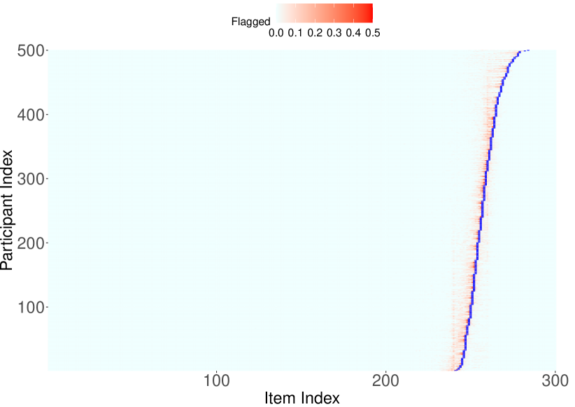
Figure D.4: Heatmap visualizing the changepoint detection performance of our proposed method when 100% of all $n$ respondents are partially careless, at significance level 0.1%. The more darker a cell in this heatmap, the more frequently across the 100 repetitions this cell was flagged as carelessness onset item ($x$-axis) of a given respondent ($y$-axis). The blue rectangles denote the true carelessness onset items (which are constant across the repetitions) and the $y$-axis is rearranged according to the location of true carelessness onset.

D.1.2 Results at Less Conservative Level

Consider again the simulation design of Section 4. Figure D.5 is equivalent to Figure 5, just with significance level 0.5% instead of 0.1%. The results are very similar to Figure 5, save for about 10% attentive respondents being incorrectly identified as careless when carelessness is extremely prevalent at 80%. We therefore do not recommend choosing a more liberal significance level that is higher than 0.1%.

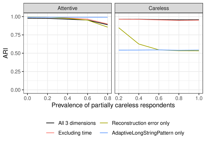
(a) ARI of fully attentive respondents against partially careless respondents.

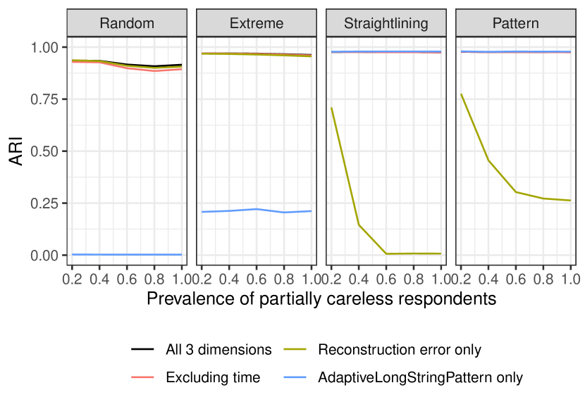
(b) ARI of each careless response style.

Figure D.5: ARI estimates in the design of Section 4 for varying carelessness prevalence, averaged over different subgroups, at significance level 0.5%.

D.1.3 Design with Strong Response Heterogeneity

This simulation design is exactly the same as in Section 4, save for two key differences. First, a simulated dataset of responses measures 10 constructs, each of which is measured by 30 items. resulting in a total of $10\times 30=300$ items (as in Section 4). Second, we alter the response probability distributions of the five answer categories. Like in Alfons & Welz, (2022), instead of the distribution in Table 1, we distinguish between four distinct types of distributions for the different constructs: centered about the midpoint, skewed towards agreeing, skewed towards disagreeing, and polarizing (likely to agree or to disagree). Table D.1 lists each distribution. All 10 items within a construct follow the same response probability distribution. We use the “centered” and “polarizing” distributions in seven constructs each, and the “agreeing” and “disagreeing“ constructs in eight constructs each, resulting in the aforementioned $10\times 2\times(7+8)=300$ items.

Type of distribution	$\mathbb{P}[X=1]$	$\mathbb{P}[X=2]$	$\mathbb{P}[X=3]$	$\mathbb{P}[X=4]$	$\mathbb{P}[X=5]$
Centered	0.15	0.20	0.30	0.20	0.15
Agreeing	0.10	0.15	0.20	0.25	0.30
Disagreeing	0.30	0.25	0.20	0.15	0.10
Polarizing	0.30	0.175	0.05	0.175	0.30

Table D.1: Response probability distributions of items within the corresponding scales. The random variable $X$ denotes the response to an item with five Likert-type answer categories (1 = “strongly disagree”, 2 = “disagree”, 3 = “neither agree nor disagree”, 4 = “agree”, 5 = “strongly agree”).

This simulation design is supposed to be very challenging for the autoencoder because it must learn response behaviors for a variety of highly heterogeneous scales, where each of which is measured by only 10 items. Consequently, the autoencoder must learn more heterogeneous responses based on less items (compared to Section 4), thereby creating an interesting challenge for our proposed method.

In the following, we present and discuss results (averaged over 100 repetitions) at significance level 0.1%.

Figure D.6: Heatmap visualizing the changepoint detection performance of our proposed method when 60% of all $n$ respondents are partially careless in the design of Appendix D.1.3, at significance level 0.1%. The more darker a cell in this heatmap, the more frequently across the 100 repetitions this cell was flagged as carelessness onset item ($x$-axis) of a given respondent ($y$-axis). The blue rectangles denote the true carelessness onset items (which are constant across the repetitions) and the $y$-axis is rearranged according to the location of true carelessness onset. An absence of a blue rectangle (occurs in 40% of all respondents) indicates that a given respondent never becomes careless.

Figure D.6 is analogous to Figure 4. We can see that our method identifies fewer careless onset items, but when it identifies changepoints, its estimates of onset location are highly accurate. Again, incorrectly detected changepoints in attentive respondents does not seem to be an issue at all.

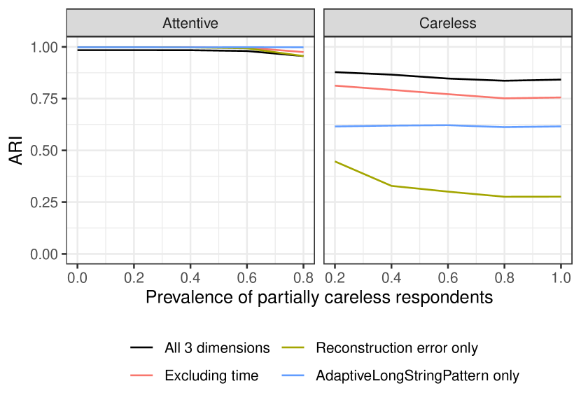
(a) ARI of fully attentive respondents against partially careless respondents.

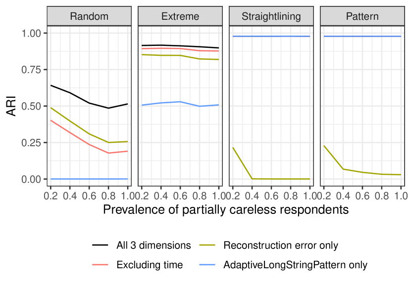
(b) ARI of each careless response style.

Figure D.7: ARI estimates in the design of Appendix D.1.3 for varying carelessness prevalence, averaged over different subgroups, at significance level 0.1%.

Figure D.7 shows ARIs for several subgroups and is analogous to Figure 5. Just like in Figure 5, our method barely ever incorrectly identifies changepoints in attentive respondents. Conversely, the ARI for careless respondents is again fairly constant across different carelessness prevalence levels with an ARI of about 0.85–0.9, which is an excellent performance, in particular when considering the difficulty of the experimental design. In addition, our method is again highly precise in accurately estimating changepoints in invariable careless respondents with near-perfect ARIs. In extreme careless responding, our method achieves an outstanding ARI of about 0.9). In random careless respondents, the ARIs are notably smaller, in particular if prevalence of carelessness is high (ARI of 0.5–0.63). This is primarily due to the extremely conservative significance level: Random carelessness behavior is arguably the hardest to detect, so our method needs to accrue high levels of evidence to identify such respondents. Combined with an extremely conservative significance level and an overall highly challenging design, our method sometimes does not identify a changepoint for some random careless respondents, which substantially drags down the ARI estimate (as such cases are awarded an ARI of zero). However, if our method estimates a changepoint in random careless respondents, its estimated location is reasonably precise. Note that it is possible to achieve substantially higher ARI values in random careless respondents by choosing a higher significance level (see Figure D.8), but—just like in Section 5—we do not recommend doing so for the sake of staying conservative, at the cost of some undetected random careless respondents.

Overall, with ARIs of 0.85–0.9 for careless respondents and almost no incorrectly flagged attentive respondents, our method performs very well at significance level 0.1% in this challenging simulation design.

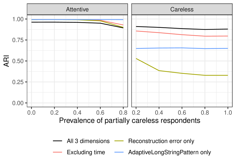
(a) ARI of fully attentive respondents against partially careless respondents.

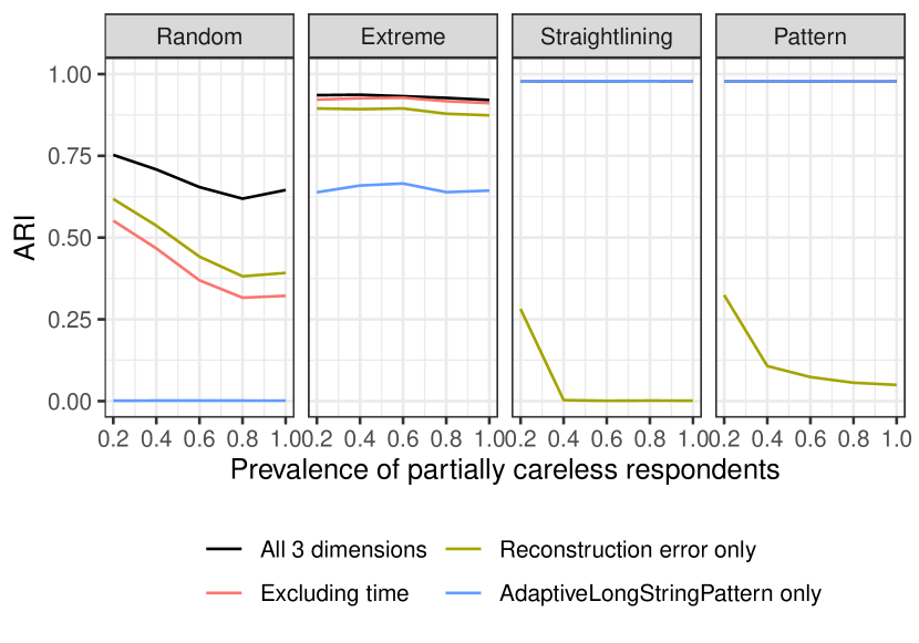
(b) ARI of each careless response style.

Figure D.8: ARI estimates in the design of Appendix D.1.3 for varying carelessness prevalence, averaged over different subgroups, at significance level 0.5%.

D.1.4 Simulated NEO-PI-R Administration

In this design, we adapt the design of Appendix D.1.3 to emulate an administration of the NEO-PI-R instrument (Costa & McCrae,, 1992). In short, this instrument comprises 240 items that measure the 30 facets of the Big 5 personality traits (see Section 5 for a detailed description). Each facet construct is measured with eight items on a five-point Likert scale. We assume that all eight items comprising a construct follow the same response probability distributions. Consider the distributions in Table D.1. We use the “centered” and polarizing distributions in seven constructs each, and the “agreeing” and “disagreeing” constructs in eight constructs each, resulting in the aforementioned $8\times 2\times(7+8)=240$ items. Half of the items in a given construct are reverse-worded. We generate responses for 500 respondents and simulate 100 datasets. Akin to previous designs, we replace a fixed proportion of responses by (partially) careless responses. We randomly sample carelessness onset to be between the 160th and 204th item; these items respectively correspond to 66.7% and 85% of all items.

Just like in the design of Appendix D.1.3, this design in supposed to be challenging because there is strong heterogeneity between constructs, just like one would expect in an empirical administration of the NEO-PI-R. However, there is less heterogeneity than in Appendix D.1.3 due to the smaller number of (heterogeneous) constructs measured.

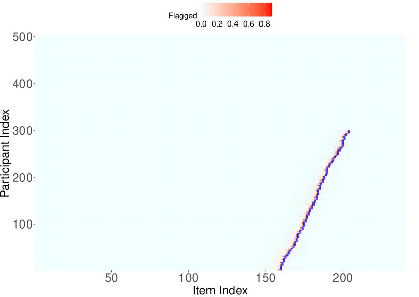
Figure D.9: Heatmap visualizing the changepoint detection performance of our proposed method when 60% of all $n$ respondents are partially careless in the design of Appendix D.1.4, at significance level 0.1%. The more darker a cell in this heatmap, the more frequently across the 100 repetitions this cell was flagged as carelessness onset item ($x$-axis) of a given respondent ($y$-axis). The blue rectangles denote the true carelessness onset items (which are constant across the repetitions) and the $y$-axis is rearranged according to the location of true carelessness onset. An absence of a blue rectangle (occurs in 40% of all respondents) indicates that a given respondent never becomes careless.

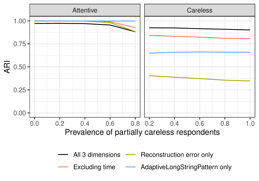
(a) ARI of fully attentive respondents against partially careless respondents.

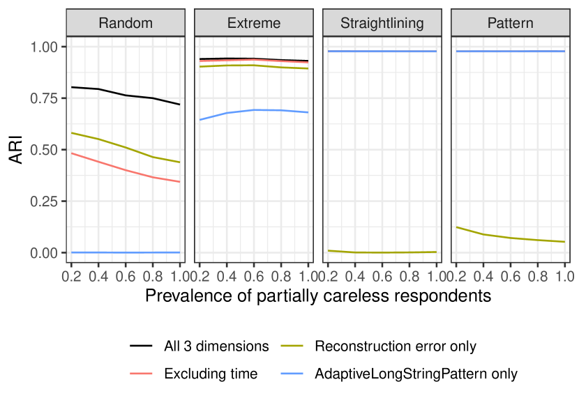
(b) ARI of each careless response style.

Figure D.10: ARI estimates in the design of Appendix D.1.4 for varying carelessness prevalence, averaged over different subgroups, at significance level 0.1%.

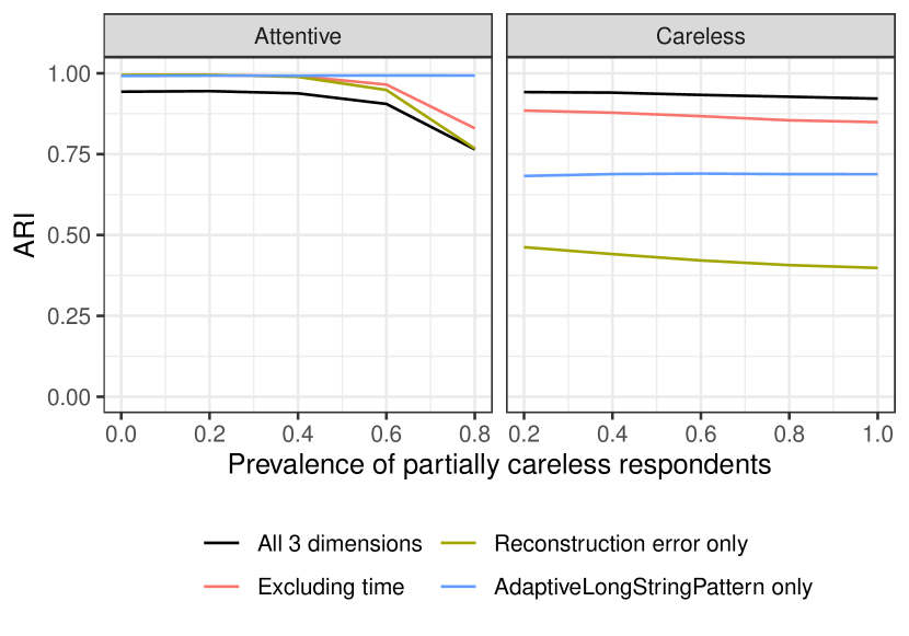
(a) ARI of fully attentive respondents against partially careless respondents.

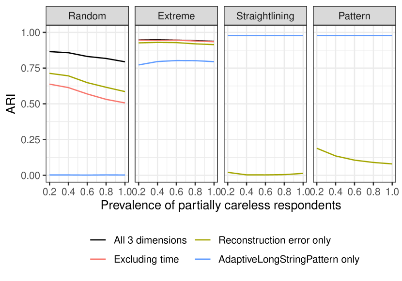
(b) ARI of each careless response style.

Figure D.11: ARI estimates in the design of Appendix D.1.4 for varying carelessness prevalence, averaged over different subgroups, at significance level 0.5%.

Figures D.9 and D.10 visualize the results at significance level 0.1%, averaged across the 100 repetitions. Figure D.11 is analogous to Figure D.10, just for significance level 0.5%.

The conclusions remain similar to the previous designs: At 0.1% level, in rarely any attentive respondents a changepoint is identified, while invariant carelessness and extreme responding are detected exceptionally accurately. Pure random responding is also identified accurately with ARIs of 0.75–0.8, but with decreasing accuracy when carelessness prevalence is high. Again, we can achieve substantially better ARIs for random responding by choosing the level to be 0.5% (see Figure D.11), but advise against this choice.

D.2 Empirical Validation

D.2.1 Application on Original Data

Figure D.12 shows the two dimensions of autoencoder reconstruction errors and AdaptiveLongstringPattern sequences, as well as test statistics associated with the single student in the data of Dolan et al., (2009) for whom our method identifies a changepoint at significance level 0.1%. When running our proposed method on both dimensions on the 400 students that have exclusively integer-valued responses, this student is the only participant in which a changepoint is identified at significance level 0.1%. The changepoint occurs at item 113, before which the reconstruction errors are strikingly larger than afterwards. There does not seem to be a structural break in the AdaptiveLongstringPattern sequences. Overall, this suggests that this student initially starts the questionnaire as inconsistent careless respondent (random-like responding), but switches to being attentive as they progress through the items.

In addition to a visual analysis of reconstruction errors and AdaptiveLongstringPattern sequences, we analyze the observed responses of the student for whom a changepoint is flagged via the their intra-individual variance (IRV). There is some evidence that carelessness manifests in low values of IRV (Dunn et al.,, 2018, in case of invariable carelessness) and high values of IRV (Marjanovic et al.,, 2015, in case of inconsistent carelessness) when when compared to IRVs of attentive respondents. We therefore compute IRVs across the items prior to a flagged changepoint and IRVs across items from the flagged changepoint onward. We do so for the student for whom a changepoint is flagged and the remaining 399 seemingly attentive participants. Table D.2 contains the corresponding IRV values. Recall from Figure D.12 that the student is suspected to start the questionnaire carelessly and that their high pre-changepoint reconstruction errors suggest inconsistent carelessness. Indeed, they have a substantially higher IRV value (1.65) in their pre-changepoint responses than post-changepoint responses (1.33), which reflects larger response variation in their suspected periods of carelessness, possibly due to random-like responding.

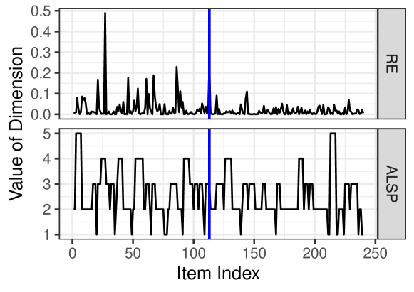
(a) Autoencoder reconstruction errors (RE) and AdaptiveLongstringPattern sequences (ALSP). A changepoint is estimated at item 113 (blue line).

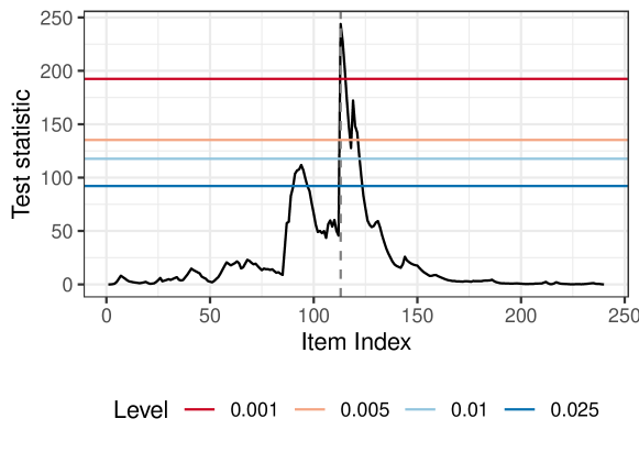
(b) Test statistic across the $p=240$ responses of the single student for whom a changepoint is identified at level 0.1%. The maximum test statistic amounts to $\hat{T_{p}}=\max_{k=1,\dots,p-1}T_{p}(k)=243.87$, which occurs at item 113 (vertical gray dashed line), using the notation of Section C.2. The colored horizontal lines denote the critical values $K_{p}$ for significance levels $\alpha=0.001,0.005,0.01,0.025$ of the maximum test statistic (Table 1 in Shao & Zhang,, 2010).

Figure D.12: Autoencoder reconstruction errors (RE), AdaptiveLongstringPattern sequences (ALSP), and test statistics of the student in the NEO-PI-R administration of Dolan et al., (2009) for whom a changepoint is found at significance level $\alpha=0.001$ when using both dimensions RE and ALSP.

	IRV careless		av. IRV attentive
CP	pre-CP	post-CP	pre-CP	post-CP
113	1.65	1.33	1.26	1.12

Table D.2: IRV calculated across subsets of observed responses of the single student for whom a changepoint is found at significance level 0.1% in the NEO-PI-R administration of Dolan et al., (2009). “CP” denotes the estimated changepoint item, “pre-CP” is the IRV calculated for items until the changepoint item, “post-CP” is the IRV calculated for items from the changepoint item onward until the last (240th) item. We report IRVs both on the individual level of the student (“IRV careless”) and the average IRV across the 399 participants without a changepoint (“av. IRV attentive”).

D.2.2 Validation With Less Conservative Level

In this subsection, we present our method’s results when applied on the data of Dolan et al., (2009) in which we have included generated careless responses. The sole difference to Section 5 is that we report results for the less conservative significance level 0.5% instead of 0.1%. Hence, Figure D.13 is equivalent to Figure 6, just when the less conservative level is used. As explained in the main text, choosing the less conservative level of 0.5% results in a noticeable improvement of the ARI for participants with random and extreme careless response styles, without a significant adverse effect of attentive respondents being incorrectly identified as careless.

(a) ARI of attentive and careless respondents.
 
 

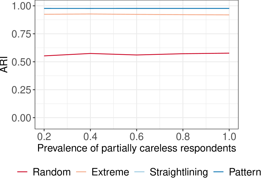
(b) ARI of each careless response style. Note that the ARIs of straightliners and pattern respondents are nearly identical, resulting in overplotted lines.

Figure D.13: ARI estimates for varying carelessness prevalence, averaged over different subgroups at significance level 0.5%, using the hybrid data based on the NEO-PI-R administration of Dolan et al., (2009). We used the two-dimensional series comprising autoencoder reconstruction errors and AdaptiveLongstringPatternsequences.

References

- Ackley et al., (1985) Ackley, D. H., Hinton, G. E., & Sejnowski, T. J. (1985). A learning algorithm for Boltzmann machines. Cognitive Science, 9(1), 147–169. https://doi.org/10.1016/S0364-0213(85)80012-4
- Alfons & Welz, (2022) Alfons, A. & Welz, M. (2022). Open science perspectives on machine learning for the identification of careless responding: A new hope or phantom menace? psyArXiv preprint psyArXiv:10.31234. https://doi.org/10.31234/osf.io/8t2cy
- Arias et al., (2020) Arias, V. B., Garrido, L., Jenaro, C., Martínez-Molina, A., & Arias, B. (2020). A little garbage in, lots of garbage out: Assessing the impact of careless responding in personality survey data. Behavior Research Methods, 52(6), 2489–2505. https://doi.org/10.3758/s13428-020-01401-8
- Arthur et al., (2021) Arthur, W., Hagen, E., & George, F. (2021). The lazy or dishonest respondent: Detection and prevention. Annual Review of Organizational Psychology and Organizational Behavior, 8(1), 105–137. https://doi.org/10.1146/annurev-orgpsych-012420-055324
- Babbie, (2020) Babbie, E. R. (2020). The Practice of Social Research (15th ed.). Cengage Learning.
- Baumgartner & Steenkamp, (2001) Baumgartner, H. & Steenkamp, J.-B. E. (2001). Response styles in marketing research: A cross-national investigation. Journal of Marketing Research, 38(2), 143–156. https://doi.org/10.1509/jmkr.38.2.143.18840
- Beach, (1989) Beach, D. A. (1989). Identifying the random responder. Journal of Psychology, 123(1), 101–103. https://doi.org/10.1080/00223980.1989.10542966
- Ben-Porath & Tellegen, (2008) Ben-Porath, Y. S. & Tellegen, A. (2008). MMPI-2-RF, Minnesota Multiphasic Personality Inventory-2 Restructured Form: Manual for administration, scoring and interpretation. University of Minnesota Press.
- Berry et al., (1992) Berry, D. T., Wetter, M. W., Baer, R. A., Larsen, L., Clark, C., & Monroe, K. (1992). MMPI-2 random responding indices: Validation using a self-report methodology. Psychological Assessment, 4(3), 340–345. https://psycnet.apa.org/doi/10.1037/1040-3590.4.3.340
- Bishop, (2006) Bishop, C. M. (2006). Pattern Recognition and Machine Learning. Information Science and Statistics. Springer.
- (11) Bowling, N. A., Gibson, A. M., Houpt, J. W., & Brower, C. K. (2021a). Will the questions ever end? Person-level increases in careless responding during questionnaire completion. Organizational Research Methods, 24(4), 718–738. https://doi.org/10.1177/1094428120947794
- Bowling et al., (2016) Bowling, N. A., Huang, J. L., Bragg, C. B., Khazon, S., Liu, M., & Blackmore, C. E. (2016). Who cares and who is careless? Insufficient effort responding as a reflection of respondent personality. Journal of Personality and Social Psychology, 111(2), 218–229. https://doi.org/10.1037/pspp0000085
- (13) Bowling, N. A., Huang, J. L., Brower, C. K., & Bragg, C. B. (2021b). The quick and the careless: The construct validity of page time as a measure of insufficient effort responding to surveys. Organizational Research Methods. https://doi.org/10.1177/10944281211056520. Forthcoming.
- Brower, (2018) Brower, C. K. (2018). Too long and too boring: The effects of survey length and interest on careless responding. Wright State University. https://corescholar.libraries.wright.edu/etd_all/1918/
- Clark et al., (2003) Clark, M. E., Gironda, R. J., & Young, R. W. (2003). Detection of back random responding: Effectiveness of MMPI-2 and personality assessment inventory validity indices. Psychological Assessment, 15(2), 223–234. https://doi.org/10.1037/1040-3590.15.2.223
- Costa & McCrae, (1992) Costa, P. T. & McCrae, R. R. (1992). Revised NEO personality inventory (NEO-PI-R) and NEO five-factor (NEO-FFI) inventory: professional manual. Psychological Assessment Resources.
- Cottrell et al., (1987) Cottrell, G. W., Munro, P., & Zipser, D. (1987). Learning internal representations from gray-scale images: An example of extensional programming. Proceedings of the Ninth Annual Conference of the Cognitive Science Society, 461–473.
- Credé, (2010) Credé, M. (2010). Random responding as a threat to the validity of effect size estimates in correlational research. Educational and Psychological Measurement, 70(4), 596–612. https://doi.org/10.1177/0013164410366686
- Curran, (2016) Curran, P. G. (2016). Methods for the detection of carelessly invalid responses in survey data. Journal of Experimental Social Psychology, 66, 4–19. https://doi.org/10.1016/j.jesp.2015.07.006
- Curran & Hauser, (2019) Curran, P. G. & Hauser, K. A. (2019). I’m paid biweekly, just not by leprechauns: Evaluating valid-but-incorrect response rates to attention check items. Journal of Research in Personality, 82. https://doi.org/https://doi.org/10.1016/j.jrp.2019.103849. Article 103849.
- De Jong et al., (2008) De Jong, M. G., Steenkamp, J.-B. E., FoxJean-Paul, & Baumgartner, H. (2008). Using item response theory to measure extreme response style in marketing research: A global investigation. Journal of Marketing Research, 45(1), 104–115. https://doi.org/10.1509/jmkr.45.1.104
- DeSimone et al., (2020) DeSimone, J. A., Davison, H. K., Schoen, J. L., & Bing, M. N. (2020). Insufficient effort responding as a partial function of implicit aggression. Organizational Research Methods, 23(1), 154–180. https://doi.org/10.1177/1094428118799486
- DeSimone & Harms, (2018) DeSimone, J. A. & Harms, P. D. (2018). Dirty data: The effects of screening respondents who provide low-quality data in survey research. Journal of Business and Psychology, 33, 559–577. https://doi.org/10.1007/s10869-017-9514-9
- DeSimone et al., (2015) DeSimone, J. A., Harms, P. D., & DeSimone, A. J. (2015). Best practice recommendations for data screening. Journal of Organizational Behavior, 36(2), 171–181. https://doi.org/10.1002/job.1962
- Dolan et al., (2009) Dolan, C. V., Oort, F. J., Stoel, R. D., & Wicherts, J. M. (2009). Testing measurement invariance in the target rotated multigroup exploratory factor model. Structural Equation Modeling, 16(2), 295–314. https://doi.org/10.1080/10705510902751416
- Dunn et al., (2018) Dunn, A. M., Heggestad, E. D., Shanock, L. R., & Theilgard, N. (2018). Intra-individual response variability as an indicator of insufficient effort responding: Comparison to other indicators and relationships with individual differences. Journal of Business and Psychology, 105–121. https://doi.org/10.1007/s10869-016-9479-0
- Edwards, (2019) Edwards, J. R. (2019). Response invalidity in empirical research: Causes, detection, and remedies. Journal of Operations Management, 65(1), 62–76. https://doi.org/10.1016/j.jom.2018.12.002
- Emons, (2008) Emons, W. H. M. (2008). Person-fit analysis of polytomous items. Applied Psychological Measurement, 32(3), 224–247. https://doi.org/10.1177/0146621607302479
- Epskamp et al., (2012) Epskamp, S., Cramer, A. O. J., Waldorp, L. J., Schmittmann, V. D., & Borsboom, D. (2012). qgraph: Network visualizations of relationships in psychometric data. Journal of Statistical Software, 48(4), 1–18. https://doi.org/10.18637/jss.v048.i04
- Galesic & Bosnjak, (2009) Galesic, M. & Bosnjak, M. (2009). Effects of questionnaire length on participation and indicators of response quality in a web survey. Public Opinion Quarterly, 73(2), 349–360. https://doi.org/10.1093/poq/nfp031
- Gibbert et al., (2021) Gibbert, M., Nair, L. B., Weiss, M., & Hoegl, M. (2021). Using outliers for theory building. Organizational Research Methods, 24(1), 172–181. https://doi.org/10.1177/1094428119898877
- Gibson & Bowling, (2020) Gibson, A. M. & Bowling, N. A. (2020). The effects of questionnaire length and behavioral consequences on careless responding. European Journal of Psychological Assessment, 36(2), 410–420. https://doi.org/10.1027/1015-5759/a000526
- Goldammer et al., (2020) Goldammer, P., Annen, H., Stöckli, P. L., & Jonas, K. (2020). Careless responding in questionnaire measures: Detection, impact, and remedies. The Leadership Quarterly, 31(4), 101384. https://doi.org/10.1016/j.leaqua.2020.101384
- Goldberg, (1992) Goldberg, L. R. (1992). The development of markers for the Big-Five factor structure. Psychological Assessment, 4(1), 26–42. https://doi.org/10.1037/1040-3590.4.1.26
- Goldberg, (1999) Goldberg, L. R. (1999). A broad-bandwidth, public domain, personality inventory measuring the lower-level facets of several five-factor models. Personality Psychology in Europe, volume 7, 7–28. Tilburg University Press.
- Goldfeld & Wujciak-Jens, (2020) Goldfeld, K. & Wujciak-Jens, J. (2020). simstudy: Illuminating research methods through data generation. Journal of Open Source Software, 5(54), 2763. https://doi.org/10.21105/joss.02763
- Goodfellow et al., (2016) Goodfellow, I., Bengio, Y., & Courville, A. (2016). Deep Learning. MIT Press. http://www.deeplearningbook.org.
- Grau et al., (2019) Grau, I., Ebbeler, C., & Banse, R. (2019). Cultural differences in careless responding. Journal of Cross-Cultural Psychology, 50(3), 336–357. https://doi.org/10.1177/0022022119827379
- Greene, (1978) Greene, R. L. (1978). An empirically derived MMPI carelessness scale. Journal of Clinical Psychology, 34(2), 407–410. https://doi.org/10.1002/1097-4679(197804)34:2<407::AID-JCLP2270340231>3.0.CO;2-A
- Hoekstra et al., (2003) Hoekstra, H., Ormel, J., & De Fruyt, F. (2003). NEO-PI-R/NEO-FFI: Big 5 persoonlijkheidsvragenlijst. Handleiding. Swets and Zeitlinger. [Manual of the Dutch version of the NEO-PI-R/NEO-FFI].
- (41) Huang, J. L., Bowling, N. A., Liu, M., & Li, Y. (2015a). Detecting insufficient effort responding with an infrequency scale: Evaluating validity and participant reactions. Journal of Business and Psychology, 30(2), 299–311. https://doi.org/10.1007/s10869-014-9357-6
- Huang et al., (2012) Huang, J. L., Curran, P. G., Keeney, J., Poposki, E. M., & DeShon, R. P. (2012). Detecting and deterring insufficient effort responding to surveys. Journal of Business and Psychology, 27(1), 99–114. https://doi.org/10.1007/s10869-011-9231-8
- (43) Huang, J. L., Liu, M., & Bowling, N. A. (2015b). Insufficient effort responding: Examining an insidious confound in survey data. Journal of Applied Psychology, 100(3), 828–845. https://doi.org/10.1037/a0038510
- Hubert & Arabie, (1985) Hubert, L. & Arabie, P. (1985). Comparing partitions. Journal of Classification, 2(1), 193–218. https://doi.org/10.1007/BF01908075
- Johnson, (2005) Johnson, J. A. (2005). Ascertaining the validity of individual protocols from web-based personality inventories. Journal of Research in Personality, 39(1), 103–129. https://doi.org/10.1016/j.jrp.2004.09.009. Proceedings of the Association for Research in Personality
- Kam & Meyer, (2015) Kam, C. C. S. & Meyer, J. P. (2015). How careless responding and acquiescence response bias can influence construct dimensionality: The case of job satisfaction. Organizational Research Methods, 18(3), 512–541. https://doi.org/10.1177/1094428115571894
- Kramer, (1991) Kramer, M. A. (1991). Nonlinear principal component analysis using autoassociative neural networks. AIChE Journal, 37(2), 233–243. https://doi.org/10.1002/aic.690370209
- Kramer, (1992) Kramer, M. A. (1992). Autoassociative neural networks. Computers & Chemical Engineering, 16(4), 313–328. https://doi.org/10.1016/0098-1354(92)80051-A
- Li et al., (2019) Li, Y., Lin, G., Lau, T., & Zeng, R. (2019). A review of changepoint detection models. arXiv preprint arXiv:1908.07136. https://arxiv.org/abs/1908.07136
- Maniaci & Rogge, (2014) Maniaci, M. R. & Rogge, R. D. (2014). Caring about carelessness: Participant inattention and its effects on research. Journal of Research in Personality, 48, 61–83. https://doi.org/10.1016/j.jrp.2013.09.008
- Marjanovic et al., (2015) Marjanovic, Z., Holden, R., Struthers, W., Cribbie, R., & Greenglass, E. (2015). The inter-item standard deviation (ISD): An index that discriminates between conscientious and random responders. Personality and Individual Differences, 84, 79–83. https://doi.org/https://doi.org/10.1016/j.paid.2014.08.021. Theory and Measurement in Personality and Individual Differences.
- McGrath et al., (2010) McGrath, R. E., Mitchell, M., Kim, B. H., & Hough, L. (2010). Evidence for response bias as a source of error variance in applied assessment. Psychological Bulletin, 136(3), 450–470. https://doi.org/10.1037/a0019216
- McNeish, (2018) McNeish, D. (2018). Thanks coefficient alpha, we’ll take it from here. Psychological Methods, 23(3), 412–433. https://doi.org/10.1037/met0000144
- Meade & Craig, (2012) Meade, A. W. & Craig, S. B. (2012). Identifying careless responses in survey data. Psychological Methods, 17(3), 437–455. https://psycnet.apa.org/doi/10.1037/a0028085
- Oppenheimer et al., (2009) Oppenheimer, D. M., Meyvis, T., & Davidenko, N. (2009). Instructional manipulation checks: Detecting satisficing to increase statistical power. Journal of Experimental Social Psychology, 45(4), 867–872. https://doi.org/10.1016/j.jesp.2009.03.009
- Peters & Gruijters, (2021) Peters, G.-J. Y. & Gruijters, S. (2021). ufs: A collection of utilities. https://r-packages.gitlab.io/ufs. R package version 0.4.5
- Rumelhart et al., (1986) Rumelhart, D. E., Hinton, G. E., & Williams, R. J. (1986). Learning internal representations by error propagation. Parallel Distributed Processing, volume 1, 318–362. http://www.cs.toronto.edu/~hinton/absps/pdp8.pdf
- Scardapane et al., (2017) Scardapane, S., Comminiello, D., Hussain, A., & Uncini, A. (2017). Group sparse regularization for deep neural networks. Neurocomputing, 241, 81–89. https://doi.org/10.1016/j.neucom.2017.02.029
- Schmitt & Stults, (1985) Schmitt, N. & Stults, D. M. (1985). Factors defined by negatively keyed items: The result of careless respondents? Applied Psychological Measurement, 9, 367–373. https://doi.org/10.1177/014662168500900405
- Schroeders et al., (2022) Schroeders, U., Schmidt, C., & Gnambs, T. (2022). Detecting careless responding in survey data using stochastic gradient boosting. Educational and Psychological Measurement, 82(1), 29–56. https://doi.org/10.1177/00131644211004708
- Shao & Zhang, (2010) Shao, X. & Zhang, X. (2010). Testing for change points in time series. Journal of the American Statistical Association, 105(491), 1228–1240. https://doi.org/10.1198/jasa.2010.tm10103
- Steinley, (2004) Steinley, D. (2004). Properties of the Hubert-Arabie Adjusted Rand Index. Psychological Methods, 9(3), 386–396. https://doi.org/10.1037/1082-989X.9.3.386
- Ward & Meade, (2022) Ward, M. & Meade, A. W. (2022). Dealing with careless responding in survey data: Prevention, identification, and recommended best practices. Annual Review of Psychology. https://doi.org/10.1146/annurev-psych-040422-045007. Forthcoming.
- Ward et al., (2017) Ward, M., Meade, A. W., Allred, C. M., Pappalardo, G., & Stoughton, J. W. (2017). Careless response and attrition as sources of bias in online survey assessments of personality traits and performance. Computers in Human Behavior, 76, 417–430. https://doi.org/10.1016/j.chb.2017.06.032
- Ward & Pond, (2015) Ward, M. & Pond, S. B. (2015). Using virtual presence and survey instructions to minimize careless responding on internet-based surveys. Computers in Human Behavior, 48, 554–568. https://doi.org/10.1016/j.chb.2015.01.070
- Woods, (2006) Woods, C. M. (2006). Careless responding to reverse-worded items: Implications for confirmatory factor analysis. Journal of Psychopathology and Behavioral Assessment, 28(3), 186–191. https://psycnet.apa.org/doi/10.1007/s10862-005-9004-7
- Yentes & Wilhelm, (2021) Yentes, R. D. & Wilhelm, F. (2021). careless: Procedures for computing indices of careless responding. https://CRAN.R-project.org/package=careless. R package version 1.2.1
- Yu & Cheng, (2019) Yu, X. & Cheng, Y. (2019). A change-point analysis procedure based on weighted residuals to detect back random responding. Psychological Methods, 24(5), 658–674. http://dx.doi.org/10.1037/met0000212
- Yuan & Lin, (2006) Yuan, M. & Lin, Y. (2006). Model selection and estimation in regression with grouped variables. Journal of the Royal Statistical Society: Series B (Statistical Methodology), 68(1), 49–67. https://doi.org/10.1111/j.1467-9868.2005.00532.x
- Zhao et al., (2021) Zhao, Z., Jiang, F., & Shao, X. (2021). Segmenting time series via self-normalization. arXiv preprint arXiv:2112.05331. https://doi.org/10.48550/arXiv.2112.05331