IFUP-TH-2023
Aspects of the Electroweak Skyrmion

Abstract

We consider certain aspects of the electroweak Skyrmion (EWS). We discuss the case of EWS with dynamical Higgs and find numerical solutions for various values of the cutoff scale. Our results are qualitatively similar to the ones present in the literature, but we find a considerable lower mass than previous studies. We discuss the quantization of the light degrees of freedom and prove that the EWS is a boson. We consider the interaction between fermions and the EWS and the transfer of fermionic charge onto the soliton. We consider the large distance structure of the soliton and the interaction between two well separated EWSs. We find that the classical EWS has a magnetic dipole moment. We discuss the lifetime of the metastable soliton. Finally, we discuss some phenomenological and cosmological consequences of our results.

1 Introduction

Solitons are local minima of the static energy functional of a field theory. Each individual soliton of a given class is labeled by a set of coordinates that describe its collective degrees of freedom e.g. its position and orientation in space. When they are quantized, they generate a Hilbert space that can be decomposed into irreducible representations of the Galileo group and of the internal symmetry group of the theory. Hence, in the low-energy limit, soliton states behave as one-particle states. Furthermore, when fermions are coupled to the constituent fields of a soliton, the soliton may acquire a fermion number, which may be non-integer and whose fractional part can be computed perturbatively. Several solitonic field configurations have been studied in the literature. Some of them are protected by a topological conservation law, that forbids their decay into the perturbative vacuum, both at the classical and at the quantum level. One of the field configurations that enjoy topological protection is the Skyrmion, a soliton of the chiral Lagrangian theory that was found [1] in an attempt to formulate a unified theory of mesons and baryons before the quark model was available. The Skyrme model was then revived starting in Ref. [2], with a work aimed to study their quantum properties. It was found that the predictions of the Skyrme model agree in general with about a 30% or better accuracy with the experimental data on baryons. Not all solitons have topological quantum numbers to protect them against decay. Some of them are just metastable states.

The electroweak Skyrmion (EWS) is a Skyrmion in the Weinberg-Salam electroweak (EW) theory that appeared in the literature for the first time in Ref. [3]. The authors assumed the presence of a new non-renormalizable term, that must be added to the electroweak Lagrangian in order to stabilize the topologically nontrivial solutions. Two years later, two articles, [4] and [5], studied numerically this possibility. The existence of multi-Skyrmion solutions was studied in Ref. [6], and the classical process of production and destruction of EWSs was studied numerically in Ref. [7]. All these works made the simplifying assumptions of a non-dynamical Higgs scalar and of a decoupled hypercharge field. The topic was revived recently in Ref. [8], where the authors performed a numerical study, relaxing the assumption of a frozen Higgs. They found the region of the parameter space that allows for the existence of the EWS, deriving an upper bound of approximately $8\leavevmode\nobreak\ {\rm TeV}$ for its mass, and they noted how the production and destruction of these states are $(B+L)$-violating processes. Other papers on the subject appeared [9, 10, 11, 12, 13], discussing in particular the possibility of the EWS as a dark matter constituent.

The present work has the aim to progress along these lines by studying some classical and quantum properties of the EWS. In particular, we find that the mass of the EWS previously found in the literature with a dynamical Higgs field was overestimated by an order of magnitude. We determine the rotational and vibrational modes of the EWS and use this to argue, together with arguments on its topology and parity, that the EWS is a spin-zero boson in its ground state. We furthermore find results on its asymptotic interactions as well as its interactions with fermions. We finally discuss some constraints from phenomenology, which can basically rule out the EWS in the semiclassical regime of parameter space.

It is organized with the following structure. In Section 2, we review the EWS with dynamical Higgs and present our new numerical results. In Section 3, we construct a Hilbert space for the collective degrees of freedom of the Skyrmion, and find its spin, statistics and other quantum numbers. In Section 4, we compute perturbatively the lepton number of the soliton. In Section 5, we find an expression for the long-distance interaction between two EWSs in the semiclassical approximation. In Section 6, some phenomenological aspects and the EWS as a dark matter candidate are discussed. We conclude in Section 7 with a discussion. We have delegated details about the breather (or oscillon) to App. A, the asymptotic interaction potential to App. B and the asymptotics of the fields to App. C.

2 The electroweak Skyrme model

The electroweak Skyrmion (EWS) is a soliton solution of the higher-derivative extension of the electroweak (EW) theory, described by the Lagrangian

$$\mathcal{L}_{\rm EWS}=\mathcal{L}_{\mathrm{EW}}+\frac{1}{8\Lambda^{4}}\mathrm{tr}\left((D_{\mu}\Phi)^{\dagger}(D_{\nu}\Phi)-(D_{\nu}\Phi)^{\dagger}(D_{\mu}\Phi)\right)^{2}\ ,$$ (1)

where $\mathcal{L}_{\rm EW}$ is the electroweak theory of Weinberg and Salam with gauge group $SU(2)_{L}\times U(1)_{Y}$, which we will briefly review:

$$\mathcal{L}_{\rm EW}=-\frac{1}{2g^{2}}\mathrm{tr}\ W_{\mu\nu}W^{\mu\nu}-\frac{1}{2g^{\prime 2}}\mathrm{tr}\ B_{\mu\nu}B^{\mu\nu}+\frac{1}{2}\mathrm{tr}\,(D_{\mu}\Phi)^{\dagger}(D^{\mu}\Phi)-\frac{\lambda}{4}\left(\mathrm{tr}(\Phi^{\dagger}\Phi)-v^{2}\right)^{2}\ ,$$ (2)

where the $SU(2)_{L}$ gauge fields are $W_{\mu}=gW_{\mu}^{a}\frac{\tau^{a}}{2}$, $a=1,2,3$, with field strength tensor $W_{\mu\nu}=\partial_{\mu}W_{\nu}-\partial_{\nu}W_{\mu}-\mathrm{i}\left[W_{\mu},W_{\nu}\right]$ and the $U(1)_{Y}$ gauge field is $B_{\mu}=g^{\prime}b_{\mu}\frac{\tau^{3}}{2}$, with field strength tensor $B_{\mu\nu}=\partial_{\mu}B_{\nu}-\partial_{\nu}B_{\mu}$. The Higgs doublet is parametrized as a $2\times 2$ complex matrix with real determinant

$$\Phi=\begin{pmatrix}\mathrm{i}\tau^{2}\phi^{*}&\phi\end{pmatrix}=\begin{pmatrix}\phi_{0}^{*}&\phi_{1}\\ -\phi_{1}^{*}&\phi_{0}\end{pmatrix}\ ,\qquad D_{\mu}\Phi=\partial_{\mu}\Phi-\mathrm{i}W_{\mu}\Phi+\mathrm{i}\Phi B_{\mu}\ .$$ (3)

With this parametrization, the $SU(2)_{L}$ group acts on the Higgs doublet as a left multiplication and the hypercharge group, is a gauged subgroup of $SU(2)_{R}$, acts as a right multiplication

$$SU(2)_{L} :\Phi\longrightarrow L\Phi\ ,\qquad W_{\mu}\longrightarrow LW_{\mu}L^{\dagger}-\mathrm{i}\partial_{\mu}LL^{\dagger}\ ,$$ (4)

$$U(1)_{Y} :\Phi\longrightarrow\Phi e^{-\mathrm{i}\varepsilon\frac{\tau^{3}}{2}}\ ,\qquad B_{\mu}\longrightarrow B_{\mu}+\frac{\tau^{3}}{2}\partial_{\mu}\varepsilon\ ,$$ (5)

the Higgs sector manifestly enjoys a global $SU(2)_{L}\times SU(2)_{R}$ symmetry, which is commonly referred to as custodial symmetry. The Higgs doublet can also be parametrized as

$$\Phi=sH\ ,\qquad s=\frac{v+h}{{\sqrt{2}}}\in\mathbb{R}\ ,\qquad H\in SU(2)\ ,$$ (6)

where $h$ describes the Higgs scalar, while the matrix $H$ describes the would-be Goldstone bosons that originate by spontaneous symmetry breaking. Passing to unitary gauge, one can eliminate $H$, the would-be Goldstone bosons, leaving no further gauge freedom. Note that the parametrization (6) is singular whenever $s(x)=0$ at any $x\in\mathbb{R}^{1,3}$, which means that the unitary gauge is generally ill-defined and fails to capture some non-perturbative phenomena, e.g. chiral anomalies. The scalar field expectation value causes a spontaneous symmetry breaking of the total gauge group $SU(2)_{L}\times U(1)_{Y}$ to its diagonal subgroup $U(1)_{\rm em}$, which acts as

$$U(1)_{\mathrm{em}}:\Phi\longrightarrow e^{+\mathrm{i}\varepsilon\frac{\tau^{3}}{2}}\Phi e^{-\mathrm{i}\varepsilon\frac{\tau^{3}}{2}}\ ,\qquad W_{\mu}\longrightarrow e^{+\mathrm{i}\varepsilon\frac{\tau^{3}}{2}}W_{\mu}e^{-\mathrm{i}\varepsilon\frac{\tau^{3}}{2}}+\frac{\tau^{3}}{2}\partial_{\mu}\varepsilon\ .$$ (7)

The perturbative spectrum consists of the fields

$$A_{\mu}=\sin{\theta_{w}}W_{\mu}^{3}+\cos{\theta_{w}}B_{\mu}\ ,\quad Z_{\mu}=\cos{\theta_{w}}W_{\mu}^{3}-\sin{\theta_{w}}B_{\mu}\ ,\quad W_{\mu}^{\pm}=\frac{1}{\sqrt{2}}\left(W_{\mu}^{1}\pm\mathrm{i}W_{\mu}^{2}\right)\ ,$$ (8)

where $\tan{\theta_{w}}=\frac{g^{\prime}}{g}$ is the Weinberg angle. $W_{\mu}^{1}$, $W_{\mu}^{2}$ and $Z_{\mu}$ acquire a mass $m_{W}=m_{Z}\cos{\theta_{w}}=\frac{gv}{2}$, while the remaining massless gauge boson $A_{\mu}$ is the gauge field of $U(1)_{\rm em}$. The Higgs mass is $m_{h}=\sqrt{2\lambda}v$. The phenomenological values of the dimensionful parameters are

$$m_{W}=80.379\,{\rm GeV}\,,\qquad m_{h}=125.1\,{\rm GeV}\,,\qquad v=246\,{\rm GeV}\ .$$ (9)

The numerical results in the rest of the paper are all done with these values fixed.

The parametrization $\Phi$ of the Higgs doublet has the advantage of providing an extremely simple form of the coupling to a fermion doublet, whose mass matrix is proportional to the identity

$$\mathcal{L}_{\mathrm{leptons}}=\bar{\psi}\mathrm{i}\not{D}\psi-y\bar{\psi}(\Phi P_{R}+\Phi^{\dagger}P_{L})\psi\ ,$$ (10)

where $y\langle\Phi\rangle=m_{\ell}\mathds{1}_{2}$ and the transformation laws of the fermions are

$$\begin{split}L\in SU(2)_{L}:&\qquad\psi_{L}\longrightarrow L\psi_{L}\ ,\qquad\quad\psi_{R}\longrightarrow\psi_{R}\ ,\\ e^{\mathrm{i}\alpha}\in U(1)_{Y}:&\qquad\psi_{L}\longrightarrow e^{\mathrm{i}Y\alpha}\psi_{L}\ ,\qquad\psi_{R}\longrightarrow e^{\mathrm{i}Y\alpha+\mathrm{i}\alpha\frac{\tau^{3}}{2}}\psi_{R}\ ,\end{split}$$ (11)

where $Y$ is the hypercharge.

Now we turn to the analysis of the topological structure of the classical field configuration space of the theory. We restrict to the subspace of static field configurations with finite energy. The energy functional of the EW part of the theory is

$$E_{\rm EW}=\int{\mathrm{d}}^{3}x\ \left[\frac{1}{g^{2}}\mathrm{tr}\ W_{0i}^{2}+\frac{1}{g^{\prime 2}}\mathrm{tr}\ B_{0i}^{2}+\frac{1}{2}\mathrm{tr}\ (D_{0}\Phi)^{\dagger}(D_{0}\Phi)\right.$$ (12)

$$\left.\mathop{+}\frac{1}{2g^{2}}\mathrm{tr}\ W_{ij}^{2}+\frac{1}{2g^{\prime 2}}\mathrm{tr}\ B_{ij}^{2}+\frac{1}{2}\mathrm{tr}\ (D_{j}\Phi)^{\dagger}(D_{j}\Phi)+\frac{\lambda}{4}\left(\mathrm{tr}(\Phi^{\dagger}\Phi)-v^{2}\right)^{2}\right].$$

From this expression, it is evident that any static field configuration with finite energy must approach to pure gauge at spatial infinity

$$W_{\mu}\underset{r\to\infty}{\longrightarrow}W_{\mu}^{\rm vac}=-\mathrm{i}H^{\dagger}\partial_{\mu}H,\qquad B_{\mu}\underset{r\to\infty}{\longrightarrow}B_{\mu}^{\rm vac}=\partial_{\mu}\varepsilon\frac{\tau^{3}}{2},\qquad\Phi\underset{r\to\infty}{\longrightarrow}\Phi^{\rm vac}=\frac{v}{\sqrt{2}}He^{-\mathrm{i}\varepsilon\frac{\tau^{3}}{2}}\ .$$ (13)

The topology of the static field configurations that satisfy these boundary conditions can be partially classified through the winding number of the $H$ field and with the Chern-Simons number of the weak gauge field

$$n_{H} =-\frac{1}{24\pi^{2}}\varepsilon_{ijk}\int{\mathrm{d}}^{3}x\ \mathrm{tr}\left(H^{\dagger}\partial_{i}H\ H^{\dagger}\partial_{j}H\ H^{\dagger}\partial_{k}H\right)\ ,$$ (14)

$$n_{\rm CS} =-\frac{1}{16\pi^{2}}\varepsilon_{ijk}\int{\mathrm{d}}^{3}x\ \mathrm{tr}\left(W_{i}W_{jk}+\frac{2\mathrm{i}}{3}W_{i}W_{j}W_{k}\right)\ .$$ (15)

The winding number $n_{H}$ is generally ill-defined. Due to the singularity of the parametrization (6), which allows $H$ to be discontinuous whenever $s(x)=0$. If, however $s(x)\neq 0$ everywhere, $n_{H}$ will be an integer thanks to the boundary conditions (34) (i.e. $\lim_{r\to\infty}H=\mathds{1}_{2}$). Instead, $n_{\rm CS}$ is an integer only when $W_{\mu}=\mathrm{i}U^{\dagger}\partial_{\mu}U$, ($U\in SU(2)$) and in this case corresponds to the winding number of $U$. $n_{H}$ and $n_{\rm CS}$ are not gauge invariant. Under gauge transformations with winding number $N$, they transform as $n_{H}\rightarrow n_{H}+N$, $n_{\rm CS}\rightarrow n_{\rm CS}+N$. Nevertheless, they can be used to construct the gauge invariant quantity $n=n_{H}-n_{\rm CS}$, which elegantly can be written as

$$n=-\frac{1}{24\pi^{2}}\varepsilon_{ijk}\int{\mathrm{d}}^{3}x\ \mathrm{tr}\left(H^{\dagger}D_{i}H\ H^{\dagger}D_{j}H\ H^{\dagger}D_{k}H+\frac{3\mathrm{i}}{2}H^{\dagger}W_{ij}D_{k}H\right)\ .$$ (16)

For the classical vacuum field configurations given in Eq. (13), $n_{\rm CS}=n_{H}=w(H)$. Topologically distinct vacua are separated by energy barriers, whose points of minimal height are unstable field configurations called sphalerons [14]. In this paper, we will use a “modified Chern-Simons” number [5, 8]:

$$n_{W}=-\frac{1}{24\pi^{2}}\int d^{3}x\;\varepsilon_{ijk}\mathrm{tr}(\mathrm{i}W_{i}W_{j}W_{k})\ ,$$ (17)

which converges to the Chern-Simons number $n_{\rm CS}$ for pure gauge configurations.

2.1 The Skyrme term

The addition of the Skyrme term to the electroweak Lagrangian has the aim to stabilize the Skyrmion in the limit in which the Higgs field and the weak gauge fields are frozen. In this subsection, we show that the Skyrme term contains (almost) the only effective operators among those of dimension six and eight, that, at least in principle, meet this requirement. The operator we are looking for:

• must not disappear in the limit $g\rightarrow 0$, when the gauge fields are pure gauge,

• must not disappear in the limit $m_{h}\rightarrow\infty$, when the Higgs doublet is frozen,

• must scale at least as $\mu^{\alpha}$ with $\alpha<3$ under dilatations in order to circumvent Derrick’s theorem.

At low energies, the physics beyond the Standard Model can be integrated out and its effects can be embedded in a momentum expansion in terms of non-renormalizable operators depending on the Standard Model fields

$$\mathcal{L}=\mathcal{L}_{\mathrm{SM}}+\sum\frac{c_{i}^{d=6}}{\Lambda^{2}}\mathcal{O}_{i}^{d=6}+\sum\frac{c_{i}^{d=8}}{\Lambda^{4}}\mathcal{O}_{i}^{d=8}+\cdots$$ (18)

There are two inequivalent ways of writing this series [15]. It can be expressed using the whole Higgs doublet $\phi$ (see Eq. (3)) as a building block, which leads to the Standard Model Effective Field Theory (SMEFT), or it can be expressed treating $h$ and $H$ (see Eq. (6)) as unrelated fields, which leads to the Higgs Effective Field Theory (HEFT). In the rest of this work, we will adopt a SMEFT-based approach. Let us first look at the operators of dimension six, in the basis of Ref. [16]:

$Q_{\phi W}$	$(\phi^{\dagger}\phi)W^{a}_{\mu\nu}W^{\mu\nu}_{a}$	$Q_{W}$	$\varepsilon_{abc}W^{a\nu}_{\mu}W^{b\rho}_{\nu}W^{c\mu}_{\rho}$
$Q_{\phi\widetilde{W}}$	$(\phi^{\dagger}\phi)W^{a}_{\mu\nu}\widetilde{W}^{\mu\nu}_{a}$	$Q_{\widetilde{W}}$	$\varepsilon_{abc}\widetilde{W}^{a\nu}_{\mu}W^{b\rho}_{\nu}W^{c\mu}_{\rho}$
$Q_{\phi B}$	$(\phi^{\dagger}\phi)B_{\mu\nu}B^{\mu\nu}$	$Q_{\phi}$	$(\phi^{\dagger}\phi)^{3}$
$Q_{\phi\widetilde{B}}$	$(\phi^{\dagger}\phi)B_{\mu\nu}\widetilde{B}^{\mu\nu}$	$Q_{\phi\square}$	$(\phi^{\dagger}\phi)\square(\phi^{\dagger}\phi)$
$Q_{\phi WB}$	$(\phi^{\dagger}\tau^{a}\phi)\widetilde{W}^{a}_{\mu\nu}B^{\mu\nu}$	$Q_{\phi D}$	$(\phi^{\dagger}D^{\mu}\phi)^{*}(\phi^{\dagger}D_{\mu}\phi)$
$Q_{\phi\widetilde{W}B}$	$(\phi^{\dagger}\tau^{a}\phi)\widetilde{W}^{a}_{\mu\nu}B^{\ \mu\nu}$

tableDimension-6 operators in the SMEFT Lagrangian involving electroweak fields.

These operators cannot stabilize the Skyrmion. All the operators that contain a field strength tensor vanish when the fields are pure gauge. The remaining operators can be excluded due to Derrick’s theorem.

We are forced to search for a suitable extension among the dimension-8 operators; the following table presents the operators that do not involve field strength tensors:

$Q_{\phi^{8}}$	$(\phi^{\dagger}\phi)^{4}$	$Q_{\phi^{4}}^{(1)}$	$(D_{\mu}\phi^{\dagger}D_{\nu}\phi)(D^{\nu}\phi^{\dagger}D^{\mu}\phi)$
$Q_{\phi^{6}}^{(1)}$	$(\phi^{\dagger}\phi)^{2}(D_{\mu}\phi^{\dagger}D^{\mu}\phi)$	$Q_{\phi^{4}}^{(2)}$	$(D_{\mu}\phi^{\dagger}D_{\nu}\phi)(D^{\mu}\phi^{\dagger}D^{\nu}\phi)$
$Q_{\phi^{6}}^{(2)}$	$(\phi^{\dagger}\phi)(\phi^{\dagger}\tau^{a}\phi)(D_{\mu}\phi^{\dagger}\tau^{a}D^{\mu}\phi)$	$Q_{\phi^{4}}^{(3)}$	$(D^{\mu}\phi^{\dagger}D_{\mu}\phi)(D^{\nu}\phi^{\dagger}D_{\nu}\phi)$

tableDimension-8 operators in the SMEFT Lagrangian involving electroweak fields.

As a consequence of Derrick’s theorem, the only operators that can stabilize the Skyrmion are $Q_{\phi^{4}}^{(1)}$, $Q_{\phi^{4}}^{(2)}$ and $Q_{\phi^{4}}^{(3)}$. The Skyrme term (1) corresponds to the particular combination of operators:

$$\mathcal{O}_{\rm Sk}=\frac{1}{2}\big{(}Q_{\phi^{4}}^{(1)}+Q_{\phi^{4}}^{(2)}-2Q_{\phi^{4}}^{(3)}\big{)}\ .$$ (19)

Custodial symmetry is satisfied as long as the coefficients of $Q_{\phi^{4}}^{(1)}$ and $Q_{\phi^{4}}^{(2)}$ are equal. In principle, by choosing different coefficients of the three operators, or by adding other operators of dimensions six and eight, it is still possible to obtain a stable soliton, and it is expected that these operators give non-negligible contributions to the EWS computation. These possibilities have been studied in Ref. [13], in the HEFT context, but will not be taken into account in the present work. Our choice has the advantage of yielding equations of motion that are linear in second-derivatives of the fields, as pointed out in Ref. [2]. We will not discuss the origin of the Skyrme term, which can be the low-energy counterpart of a variety of renormalizable extensions of the Standard Model [8], in particular of those including massive fermions [17, 18, 19].

2.2 The electroweak Skyrmion solution

The Ansatz for the weak gauge field configuration is chosen to be spherically symmetric

$$W_{i}(\textbf{x})=g\frac{\tau^{a}}{2}\left[\varepsilon_{aij}\hat{x}_{j}\frac{f_{1}(r)}{r}+(\delta_{ia}-\hat{x}_{i}\hat{x}_{a})\frac{f_{2}(r)}{r}+\hat{x}_{i}\hat{x}_{a}\frac{b(r)}{r}\right],\qquad W_{0}(\textbf{x})=0\ .$$ (20)

Field configurations of this kind have the nice property of being invariant under combined global $SU(2)_{L}$ and spatial $SO(3)$ transformations

$$W_{i}^{(D)}(\textbf{x})=D_{ji}W_{j}(D\textbf{x})=AW_{i}(\textbf{x})A^{\dagger}\ ,\qquad D\in SO(3)\ ,\ A\in SU(2)$$ (21)

The Higgs field configuration is chosen to be of the form

$$\Phi(\textbf{x})=\frac{v\sigma(r)}{\sqrt{2}}\mathds{1}_{2}\ ,$$ (22)

which is invariant under spatial rotations and under $SU(2)_{\mathrm{diag}}\subset SU(2)_{L}\times SU(2)_{R}$ transformations. Therefore, in this gauge the solution has zero Higgs winding number, and is characterized by its Chern-Simons number only.

We briefly review some previous results on this topic. The solutions have been studied in the literature in the limit where the Higgs field [4, 5, 7] or the gauge fields [10] are frozen. When both limits are taken $(g\rightarrow 0,m_{h}\rightarrow\infty)$, the Lagrangian takes the form

$$\mathcal{L}=\frac{v^{2}}{4}\mathrm{tr}\ (\partial_{\mu}H)^{\dagger}(\partial^{\mu}H)+\frac{v^{4}}{32\Lambda^{4}}\mathrm{tr}\left[H^{\dagger}\partial_{\mu}H,H^{\dagger}\partial_{\nu}H\right]^{2},$$ (23)

which is a scaled-up version of the Skyrme Lagrangian with massless mesons. In this reduced model, the Skyrmion mass would be

$$M_{\rm EWS}\simeq 23.2\,\pi\frac{v^{3}}{\Lambda^{2}}\approx\frac{10^{5}\ {\rm GeV}}{(\Lambda/100\ {\rm GeV})^{2}}\;,$$ (24)

and its lifetime infinite. In Ref. [5] the authors work under assumption of non-dynamical Higgs and dynamical gauge fields ($g\neq 0,m_{h}\to\infty$). The results are expressed as a function of the dimensionless parameter $\xi=\frac{4\Lambda^{4}}{g^{2}v^{4}}$. It was found that the Skyrmion has a mass [5]

$$\xi_{\rm crit}\simeq 10\ ,\qquad\Lambda_{\rm crit}\simeq 250\ {\rm GeV}\ ,\qquad M_{\rm EWS}\simeq 15\ {\rm TeV}\ .$$ (25)

where $\xi_{\rm crit}$ and $\Lambda_{\rm crit}$ are the lowest values of the parameter $\xi$ and $\Lambda$ for which the EWS is classically stable (see Sec. 2.5 for a more detailed discussion). In Ref. [8] the EWS is studied using the most general assumptions of dynamical Higgs and gauge fields ($g\neq 0,m_{h}\neq\infty$). The shape of the Skyrmion was obtained as a function of the modified Chern-Simons number $n_{W}$ of the field configuration at fixed $\Lambda$, by introducing the Lagrange multiplier $\lambda$ and minimizing the functional:

$$E_{\lambda}=E-\lambda\big{(}n_{W}-n_{W}^{(\rm Sk)}\big{)}\ .$$ (26)

In this way, one can obtain the energy of the EWS (if the solution exists) as a function of $\Lambda$ in parameter space, and of $n_{W}$ in field configuration space. In Ref. [8] the Skyrmion mass and radius relations were obtained:

$$M\simeq 0.35\frac{4\pi v^{3}}{\Lambda^{2}}\ ,\qquad R\simeq 0.6\frac{v}{\Lambda^{2}}\ ,$$ (27)

and the mass is minimized quite close to, but not exactly at $n_{W}=1$. All current literature considers the $U(1)_{Y}$ fields decoupled ($g^{\prime}=0,B_{\mu}=0$) at the zeroth order of the semiclassical approximation. This assumption is reasonable as long as $g^{\prime}\ll g$, which is true in nature as $\sin^{2}{\theta_{\mathrm{W}}}\simeq 0.223$.

2.3 Numerical results

The shape of the EWS can be determined by minimizing the integral obtained by substituting the spherically symmetric Ansatz (20) into the static energy functional of the theory (1). Thanks to spherical symmetry, the resulting integral is one dimensional, and the integrand is a polynomial in $f_{1}(r),f_{2}(r),b(r)$, $\sigma(r)$ and their first derivatives:

$$E=\frac{4\pi v^{3}}{\Lambda^{2}}E_{\rm nat}\ ,$$ (28)

with the dimensionless energy functional

$$E_{\rm nat}=\int{\mathrm{d}}r \Bigg{\{}\alpha\left[\left(f_{1}^{\prime}-2f_{2}\frac{b}{r}\right)^{2}+\left(f_{2}^{\prime}+(2f_{1}-1)\frac{b}{r}\right)^{2}+\frac{2}{r^{2}}\left(f_{1}^{2}+f_{2}^{2}-f_{1}\right)^{2}\right]$$

$$+\frac{r^{2}}{2}(\sigma^{\prime})^{2}+\sigma^{2}\left(f_{1}^{2}+f_{2}^{2}+\frac{b^{2}}{2}\right)+\beta r^{2}(\sigma^{2}-1)^{2}$$

$$+(f_{1}^{2}+f_{2}^{2})\sigma^{2}\left[(\sigma^{\prime})^{2}+\frac{\sigma^{2}}{r^{2}}\left(b^{2}+\frac{f_{1}^{2}+f_{2}^{2}}{2}\right)\right]\Bigg{\}},$$ (29)

where we have performed the rescaling [8] of the radial coordinate by $r\to\frac{v}{\Lambda^{2}}r$ and the fields by $(f_{1},f_{2},b)\to\frac{2}{g}(f_{1},f_{2},b)$ and we have defined

$$\alpha=\frac{\Lambda^{4}}{v^{2}m_{W}^{2}}\ ,\qquad\beta=\frac{m_{h}^{2}v^{2}}{8\Lambda^{4}}\ .$$ (30)

Note that in this functional there are no derivatives of $b$, which therefore is not a proper dynamical variable but a Lagrange multiplier and can be solved algebraically

$$b=\frac{2r\alpha(2f_{2}f_{1}^{\prime}+(1-2f_{1})f_{2}^{\prime})}{2\alpha((1-2f_{1})^{2}+4f_{2}^{2})+r^{2}\sigma^{2}+2(f_{1}^{2}+f_{2}^{2})\sigma^{4}}\ .$$ (31)

The corresponding Euler-Lagrange equations

$$f_{i}^{\prime\prime}-\frac{1}{8\pi\alpha}\frac{\partial E_{\rm nat}}{\partial f_{i}} =\ddot{f}_{i}\ ,\qquad i=1,2,\$$ (32)

$$\sigma^{\prime\prime}-\frac{1}{4\pi(r^{2}+2(f_{1}^{2}+f_{2}^{2})\sigma^{2})}\frac{\partial E_{\rm nat}}{\partial\sigma} =\ddot{\sigma}\ ,$$ (33)

must be solved numerically with the boundary conditions

$$\begin{split}f_{1}(0)=&f_{1}^{\prime}(0)=f_{2}(0)=b(0)=f_{2}^{\prime}(0)-b^{\prime}(0)=\sigma^{\prime}(0)=0\ ,\\ &f_{1}(\infty)=f_{2}(\infty)=b(\infty)=\sigma(\infty)-1=0\ ,\end{split}$$ (34)

which ensure the finiteness of the energy and the regularity at the origin.

The modified Chern-Simons number for this configuration in dimensionless coordinates is

$$n_{W}=\frac{2}{\pi}\int\frac{1}{r}{\mathrm{d}}r\ (f_{1}^{2}+f_{2}^{2})b\ .$$ (35)

In order to solve the field equations, mathematically we could eliminate $b$ algebraically, but it turns out not to be the best way for the numerical methods we have utilized. Our numerical method is the following. We solve the second-order differential equations (32)-(33) using the arrested Newton-flow and updating $b$ by its exact solution (31) at every step. The arrested Newton-flow algorithm works by evolving the flow “time” and evaluating the potential energy $E_{\rm nat}[f_{1},f_{2},\sigma]$ at every step, setting the first flow-time derivative to zero ($\dot{f}_{1}=\dot{f}_{2}=\dot{\sigma}=0$) if $E_{\rm nat}$ increases. At every step, $b$ is updated using its exact solution (31). We measure the right-hand side of the equations and after they integrate to a number smaller than $10^{-6}$, we stop the flow and the numerical solution has been obtained. Contrary to claims in the literature, we do not need to restrict the fields to a specific Chern-Simons number if our initial guess is close enough to the correct solution.

In order to define the size or radius of the EWS, we define the following mean-squared functional

$$r_{X}^{2}:=\frac{\int{\mathrm{d}}r\ r^{4}X}{\int{\mathrm{d}}r\ r^{2}X}\ ,$$ (36)

where we can take $X$ to be the energy density $X=\mathcal{E}$, the Chern-Simons density $X=\mathcal{Q}_{W}$ or simply $X=(1-\sigma)^{2}$.

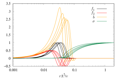
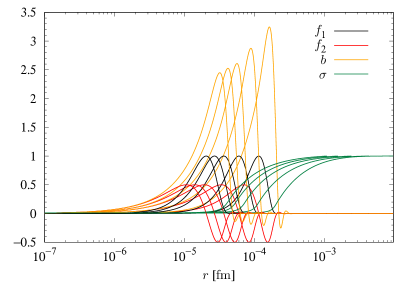
Figure 1: Electroweak Skyrmion profile functions for different values of $\Lambda=100,150,200,250,300$ GeV, corresponding to the curves from left to right (right to left) in the left (right) figure, plotted as functions of the log radius $r\Lambda^{2}/v$ ($r$). The modified Chern-Simons charge is localized where the Higgs field vanishes.

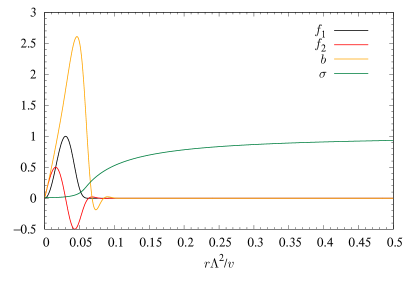
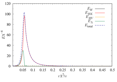
Figure 2: Electroweak Skyrmion profile functions (left) and energy densities (right) for $\Lambda=200$ GeV.

(a)

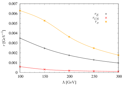
(b)

Figure 3: Mass (left) and radius (right) in GeV (GeV^-1) for the different EWSs of Fig. 1. Three different definitions of the radius are shown, where Eq. (36) is used with the energy density, the modified Chern-Simons density and $(1-\sigma)^{2}$, respectively.

(a)

(b)

Figure 4: (a) Modified Chern-Simons number (35) for the solutions of Fig. 1. They are so close to one for the entire range of $\Lambda$, that we cannot determine whether they are not exactly equal to one from their numerical error. (b) Energy of the YM tensor in GeV for the same solutions.

We now present our numerical results. In Fig. 1 we show the profile functions $f_{1}$, $f_{2}$, $b$, and $\sigma$ for various values of $\Lambda$ in the range $\Lambda\in[100,300]\leavevmode\nobreak\ {\rm GeV}$. The smaller $\Lambda$ is, the smaller is the size of the solution in dimensionless coordinates. This is an artifact of the dimensionless units, because in physical units when restoring $v/\Lambda^{2}$, the solutions do shrink as $\Lambda$ is increased. In Fig. 2(a) the profile functions are shown in a non-log scale plot for $\Lambda=200\leavevmode\nobreak\ {\rm GeV}$, whereas in Fig. 2(b) the corresponding energy density is shown. In Fig. 3(a), the energy of the EWS is shown in GeV as a function of $\Lambda$. The energy or mass of the EWS clearly decreases as $\Lambda$ increases, as one would expect.

In Fig. 3(b), the radius of the EWS is shown in fm according to various definitions of the density used as a measure and for the range of $\Lambda$ used for the solutions in Fig. 1. The radius of the EWS lies in the $10^{-3}$-$10^{-4}$ fm range and shrinks as the scale $\Lambda$ is increased. We can also see that the energy density is about an order of magnitude more extended than the modified Chern-Simons density; this is largely due to the tail of the Higgs field. Approximate relations of the energy and radius obtained with the energy density as functions of $\Lambda$ and $v$ are given by

$$M \simeq\left(0.0130+\frac{\Lambda}{16.9\ {\rm TeV}}\right)\frac{4\pi v^{3}}{\Lambda^{2}}\ ,$$

$$r_{E} \simeq\left(-0.0749+\frac{\Lambda}{390\ {\rm GeV}}-\frac{\Lambda^{2}}{(513\ {\rm GeV})^{2}}\right)\frac{v}{\Lambda^{2}}\ .$$ (37)

Finally, in Fig. 4(a) we show the modified Chern-Simons number (35) for the solutions of Fig. 1. This number is always very close to one. Since the number is so close to unity, we cannot determine whether it is smaller than one or that is simply the numerical error of the solution. In Fig. 4(b), we display the energy of the YM field strength tensor, which can be seen to be four orders of magnitude smaller than the mass of the EWS for $\Lambda\geq 150\,{\rm GeV}$. This means that the gauge field $W_{i}$ is very close to being pure gauge, which explains why $n_{W}$ is so close to unity.

We find here that in Ref. [8] both the mass and the radius are overestimated by more than an order of magnitude, probably due to the numerical method utilized in that work.

2.4 Quantum and higher-derivative corrections

An important comment in store is about quantum corrections. In Fig. 3(a), we notice that around $\Lambda\approx 200\leavevmode\nobreak\ {\rm GeV}$, the mass of the EWS becomes of the order of the Higgs mass, and thus of the scale of the most massive perturbative particle. We can thus say that at this scale there is a threshold for the soliton transitioning from a (semi-)classical object to a quantum soliton. Another way to infer this is to estimate when the Compton wave length of the soliton $\lambda_{\mathrm{Compton}}\sim\frac{1}{M}$ becomes of the same order of the soliton size. Using the relations (37) we have $\frac{1}{M}\sim R$ for $\Lambda\simeq 130\ {\rm GeV}$.

The Lagrangian (1) defines an effective field theory with a physical cutoff $\Lambda$. In order for our treatment to be consistent, we need to have $R\gg\frac{1}{\Lambda}$. The $r_{\sigma}$ notion in Fig. 3(b), which is the most adequate to compare higher-derivative corrections, is consistently of the same order of $\frac{1}{\Lambda}$. Therefore, we must conclude that for these values of $\Lambda$, a fully consistent treatment of the EWS requires a more detailed knowledge of the UV completion of the SMEFT Lagrangian. This is very similar to what happens for the Skyrmion in QCD with higher-derivative corrections. Corrections are expected to be important and of order one, but still under control.

2.5 Stability of the EWS

A soliton is classically stable if it is a local minimum of the energy in field configuration space. The classical stability of the EWS depends on the value of the parameter $\Lambda$. We briefly review the previous results on this topic. As we already observed, in the limit $g\to 0,m_{h}\to\infty$, the EWS corresponds to a rescaled version of the QCD Skyrmion, and hence is completely stable. In Ref. [5], under the assumption of non-dynamical Higgs ($g\neq 0,m_{h}\to\infty$) the classical stability criterion of the Skyrmion is found to be

$$\xi\geq\xi_{\rm crit}\simeq 10.35\ ,\qquad M\lesssim 15\ {\rm TeV}\ .$$ (38)

where $\xi=\frac{4\Lambda^{4}}{g^{2}v^{4}}$. On the other hand, using a dynamical Higgs field, Ref. [8] found that classically stable solutions exist only for $\Lambda\geq\Lambda_{\rm crit}\simeq 90\ \mathrm{GeV}$, which leads to the following upper bound on the mass

$$M\lesssim 8\ {\rm TeV}\ .$$ (39)

The decay of the EWS can also happen through quantum effects: if the EWS has no topological quantum number (which is the case) it can decay by tunneling through the barrier that separates it from the perturbative vacuum. There are at least two decay channels. Let us consider for simplicity a solitonic field configuration with $(n_{W},n_{H})\simeq(1,0)$. We have the following possibilities

• The EWS can tunnel to the vacuum with $(n_{W},n_{H})_{\mathrm{vac}}=(0,0)$ with a change of the (modified) Chern-Simons number only.

• The EWS can tunnel to the vacuum with $(n_{W},n_{H})_{\mathrm{vac}}=(1,1)$ with a change of the Higgs winding number only.

These two processes are not equivalent, and, in general, happen at different rates. This can be seen by taking the limit, $m_{h}\rightarrow\infty$, in which the Higgs field is frozen at its vacuum expectation value: if we increase $m_{h}$, the fluctuations of the Higgs field are more and more suppressed, and the energy barrier between two field configurations that differ by one unit of $n_{H}$ only becomes higher and higher. When $m_{h}$ is infinite, $n_{H}$ becomes a topological invariant and the above-mentioned energy barrier becomes infinite, making tunneling in that direction impossible. An estimate of the decay rate of the EWS has been made in Ref. [21] under the assumption of a frozen Higgs field. As the discussion above implies, this estimate completely misses decay processes of the second kind. The dynamical Higgs has two competing effects on the stability of the EWS. On one hand it lowers its mass rendering it more stable. On the other hand it opens new decay possibilities, in other words it lowers also the potential barrier. To compute this properly, at least in the semiclassical limit, it is necessary to find the bounce solution.

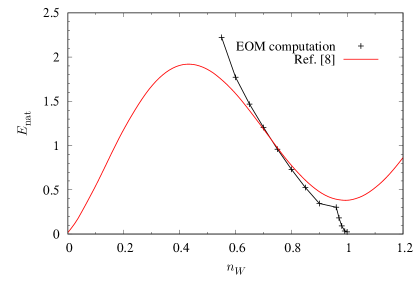
Figure 5: Dimensionless energy of EWS as a function of the modified Chern-Simons number ($n_{W}$) for $\Lambda=200\ {\rm GeV}$. The black dots represent solutions calculated with the EOM for the constrained problem, whereas the red curve is taken from Ref. [8].

In order to make an estimate, we attempt to flow the solution in field configuration space from $(n_{W},n_{H})\simeq(1,0)$ to $(n_{W},n_{H})\simeq(0,0)$, since this is the simplest and possible by utilizing the additional Lagrange multiplier term (26) and changing the Chern-Simons number from unity to zero. This flow of solutions will estimate the height of the barrier of one of the decay modes, which we estimate to be around 2 ${\rm TeV}$, see Fig. 5. We note that our flow solution became difficult to follow for $n_{W}\lesssim 0.55$; since the region in field configuration space $0.6<n_{W}<0.9$ our results are quite similar to those of Ref. [8], their barrier height is most likely correct. Since $\sim 2\ {\rm TeV}\gg 0.117\ {\rm TeV}$, with the latter being our result for the EWS mass at $\Lambda=200\ {\rm GeV}$, we can utilize the instanton approximation for the bound for estimating the lifetime of the EWS [21]:

$$\tau\approx M_{W}^{-1}e^{\frac{16\pi^{2}}{g^{2}}}\approx 3.2\times 10^{134}\ {\rm s}\ .$$ (40)

Notice that the approximate agreement between our results and those of Ref. [8] stops to hold for $0.95<n_{W}\leq 1$, where the solution decreases significantly in energy. For a more accurate estimate of the lifetime of the EWS, it is necessary to find a bounce solution that can describe the unwinding of both the Higgs field and the gauge fields. We propose the spherically symmetric Ansatz

$$\begin{split}W_{i}^{a}(\textbf{x},\tau)&=\varepsilon_{aij}\hat{x}_{j}\frac{f_{1}(r,\tau)}{r}+(\delta_{ia}-\hat{x}_{i}\hat{x}_{a})\frac{f_{2}(r,\tau)}{r}+\hat{x}_{i}\hat{x}_{a}\frac{b(r,\tau)}{r}\\ W^{a}_{0}(\textbf{x},\tau)&=\hat{x}_{a}f_{0}(r,\tau)\ ,\qquad\Phi(x)=\frac{v}{\sqrt{2}}\left[\sigma(r,\tau)\mathds{1}_{2}+\tau^{a}\beta_{a}(r,\tau)\right]\ ,\end{split}$$ (41)

where $\tau$ in the profile functions is Euclidean time. The Euclidean equations of motion must be solved with the usual boundary conditions of a bounce. Notice that the parametrization of the Higgs field is nonsingular, which allows this solution to describe the two decay channels mentioned above.

We now make an estimate of the height of the sphaleron barrier with a different method. We note that if the Higgs field vanishes, the gauge field configuration – if pure gauge – is both scale invariant and deformable to a configuration with vanishing winding number. While a scale transformation, i.e. $r\to\mu r$, does not change the winding number, a deformation $f_{1}\to\mu f_{1}$ with $f_{2}=\sqrt{f_{1}(1-f_{1})}$ (from Eq. (2.3)) and $b$ given by Eq. (31) with $\sigma=0$ can change the winding number to zero. We assume here that the gauge field configuration that we have found is so close to pure gauge, that we can assume that the latter deformation holds, and we only need to disentangle the tails from the Higgs field to be able to unwind the Skyrmion. We push the Higgs field to be zero for $r\in[0,0.1]$ for the $\Lambda=200$ GeV configuration, and determine the energy of this deformation

$$E_{\rm nat}^{\rm Higgs,\;deform}=\int{\mathrm{d}}r\left[\frac{r^{2}}{2}(\sigma^{\prime})^{2}+\beta r^{2}(\sigma^{2}-1)^{2}\right],\qquad\sigma(r_{\rm min})=\sigma^{\prime}(r_{\rm min})=0,\quad r_{\rm min}=0.1\ .$$ (42)

We find $E_{\rm nat}^{\rm Higgs,\;deform}\sim 0.1491$, which corresponds to $698$ GeV in physical units. This value is somewhat smaller than the estimate made with the equations of motion shown in Fig. 5, but we are here neglecting the fact that the gauge fields are not exactly pure gauge. We thus believe that the estimate $\approx 2$ TeV is quite reasonable.

3 Quantization of collective coordinates

The collective coordinates of the EWSs can be quantized following the procedure outlined in Refs. [22, 23] step-by-step, and using the property (21).

3.1 Rotations and isorotations

The rotational collective coordinates of the EWS correspond to the symmetries broken by the soliton and unbroken by the vacuum. This symmetry group consists of the spatial rotations and of the diagonal isospin. These transformations act on $W_{i}$ according to Eq. (21), and leave $\Phi$ invariant. If $A,L\in SU(2)$ are the matrices that parametrize rotations and diagonal isorotations respectively, the Lagrangian for the corresponding collective degrees of freedom is

$$L_{\text{rot}}=-E_{0}+\lambda\ \mathrm{tr}\big{[}\dot{(LA)}^{\dagger}\dot{(LA)}\big{]}\ ,\qquad\lambda=\frac{8\pi v^{3}}{3m_{W}^{2}\Lambda^{2}}\int_{0}^{\infty}{\mathrm{d}}r\ \left(2f_{1}^{2}+2f_{2}^{2}+b^{2}\right)\ ,$$ (43)

where $E_{0}$ is the classical energy of the EWS and $\lambda$ is the moment of inertia and the coordinates and fields have been rescaled as in Sec. 2.3.

Figure 6: Moment of inertia, $\lambda$, of Eq. (43) for the solutions of Fig. 1.

In Fig. 6 we show the moment of inertia of the EWS for the solutions of Fig. 1. Like the size of the EWS, it shrinks as $\Lambda$ is increased. An approximate relation for moment of inertia as a function of $v$ and $\Lambda$ is given by

$$\lambda \simeq\left(26.88+\frac{\Lambda}{14.08{\rm GeV}}\right)\frac{v^{3}}{m_{W}^{2}\Lambda^{2}}\ .$$ (44)

This Lagrangian describes a $(0+1)$-dimensional gauge theory with local symmetry $A\mapsto U^{\dagger}A$, $L\mapsto LU$, where $U\in SU(2)$ is time dependent. We can use this gauge freedom to impose the condition $L=\mathds{1}_{2}$. In this way, our Lagrangian further simplifies to

$$L_{\text{rot}}=-E_{0}+\lambda\,\mathrm{tr}\big{(}\dot{A}^{\dagger}\dot{A}\big{)}\ .$$ (45)

The quantization of a scalar field on a 3-sphere is well known [2, 23] for the spherically symmetric problem of the single Skyrmion. The generators of rotation and weak isorotations can be constructed as

$$I_{a}=\mathrm{i}\lambda\,\mathrm{tr}\big{(}\dot{A}A^{\dagger}\tau_{a}\big{)},\qquad J_{a}=-\mathrm{i}\lambda\,\mathrm{tr}\big{(}A^{\dagger}\dot{A}\tau_{a}\big{)}\ ,$$ (46)

which are $\mathfrak{su}(2)$ algebra-valued, mutually commute and identically satisfy $I^{2}=J^{2}$. Canonical quantization yields the rotational Hamiltonian

$$H_{\mathrm{rot}}=E_{0}+\frac{I^{2}}{2\lambda}=E_{0}+\frac{I(I+1)}{2\lambda}\ ,$$ (47)

where the eigenvalue of the squared operator of weak isospin is $I(I+1)$.

3.2 Breather mode

Although technically it is not a collective coordinate, we also quantize the breather mode. We define a scale transformation as follows

$$W_{i}(\textbf{x})\longmapsto\eta W_{i}(\eta\textbf{x})\ ,\qquad\Phi(\textbf{x})\longmapsto\Phi(\eta\textbf{x})\ ,$$ (48)

where $\eta$ is a time-dependent quantity that parametrizes the transformation. Note that, according to this transformation law, spatial components of covariant derivatives scale as

$$D_{i}\Phi(x)\longmapsto\eta D_{i}\Phi(\eta x)\ .$$ (49)

In order to have $D_{0}\Phi(x)\longmapsto\eta D_{0}\Phi(\eta x)$, we must also let $W_{0}$ acquire a spherically symmetric nontrivial value, that we parametrize as

$$W_{0}(\textbf{x})=g\frac{\dot{\eta}}{\eta}\xi(\eta r)\ \hat{x}_{a}\frac{\tau_{a}}{2}\ .$$ (50)

We now plug the transformed fields into the action (1), which yields a kinetic part due to $\eta=\eta(t)$ and the potential part of the action pics up both positive and negative powers of $\eta$.

First we need to determine the new profile function $\xi$, which turns out to be exactly solved by $\xi=b$, with $b$ given by the solution (31) in terms of $f_{1}$, $f_{2}$ and $\sigma$. Next we can determine the characteristic frequency of oscillations, which is the breather mode. Expanding in small perturbations $\epsilon=\eta-1$, we obtain the breather frequency

$$\omega_{c}=\sqrt{\frac{2B_{\text{nat}}+12C_{\text{nat}}}{D_{1,\rm nat}+D_{2,\rm nat}}}\ ,$$ (51)

with the functionals

$$B_{\rm nat} =\int_{0}^{\infty}{\mathrm{d}}r\left[\frac{r^{2}}{2}(\sigma^{\prime})^{2}+\sigma^{2}\left(f_{1}^{2}+f_{2}^{2}+\frac{b^{2}}{2}\right)\right],$$

$$C_{\rm nat} =\int_{0}^{\infty}{\mathrm{d}}r\;\beta r^{2}(\sigma^{2}-1)^{2},$$

$$D_{1,\rm nat} =\int_{0}^{\infty}r^{2}{\mathrm{d}}r\bigg{\{}2\alpha\bigg{[}\left(f_{1}^{\prime}-\frac{2b}{r}f_{2}\right)^{2}+\left(f_{2}^{\prime}+(2f_{1}-1)\frac{b}{r}\right)^{2}\bigg{]}$$

$$\phantom{=\int_{0}^{\infty}r^{2}{\mathrm{d}}r\bigg{\{}\ }+2(f_{1}^{2}+f_{2}^{2})\sigma^{2}\left((\sigma^{\prime})^{2}+\frac{\sigma^{2}}{r^{2}}b^{2}\right)\bigg{\}},$$

$$D_{2,\rm nat} =\int_{0}^{\infty}r^{2}{\mathrm{d}}r\left(r^{2}(\sigma^{\prime})^{2}+b^{2}\sigma^{2}\right).$$ (52)

For further details on this derivation, see App. A.

Figure 7: The breather frequency, $\omega_{c}$ (in ${\rm GeV}$) for the solutions of Fig. 1.

Fig. 7 shows the breather frequency for the solutions of Fig. 1 in ${\rm GeV}$, which in physical units grows nearly linearly with $\Lambda$. A fit for $\omega_{c}$ is:

$$\omega_{c}\simeq 277.917\,{\rm GeV}-0.23092\Lambda+0.00907898\frac{\Lambda^{2}}{{\rm GeV}}\ .$$ (53)

3.3 Parity

Let us now consider the action of parity on the collective modes. For a time-independent vector field, parity changes the overall sign of both the argument and of its spatial part (in 3-dimensional space), and the argument of the temporal part

$$P:\ W_{0}(\textbf{x})\longmapsto W_{0}(-\textbf{x})\ ,\qquad W_{i}(\textbf{x})\longmapsto-W_{i}(-\textbf{x})\ .$$ (54)

Performing this transformation on the Skyrmion field, one sees that its effect consists in changing the sign of $f_{2}$ and $b$. It is easy to see that this transformation cannot be reabsorbed by a transformation of any of the collective coordinates $A$ and $\varepsilon$, and that the EWS defined above does not seem to have a definite parity. The action of parity can be interpreted as follows: the Skyrmion is not sent to a rotated version of itself, but rather to a new field configuration that we can call the anti-Skyrmion. We can add a further quantum number $\uparrow$ $\downarrow$ that specifies whether the field configuration is a Skyrmion or an anti-Skyrmion, and that transforms as

$$P\ket{\uparrow}=\ket{\downarrow}\ ,\qquad P\ket{\downarrow}=\ket{\uparrow}\ .$$ (55)

The parity operator $P$ is diagonal in the rotated basis

$$\ket{\pm}=\frac{\ket{\uparrow}\pm\ket{\downarrow}}{\sqrt{2}}\ .$$ (56)

The parity operator $P$ commutes with all the rotation generators (46). The profile functions $f_{1}(r)$, $f_{2}(r)$ and $b(r)$ must be formally promoted to commuting operator-valued functions $\hat{f}_{1}(r)$, $\hat{f}_{2}(r)$ and $\hat{b}(r)$ such that

$$\begin{split}&\hat{f}_{1}\ket{\uparrow}=+f_{1}\ket{\uparrow}\ ,\qquad\hat{f}_{2}\ket{\uparrow}=+f_{2}\ket{\uparrow}\ ,\qquad\hat{b}\ket{\uparrow}=+b\ket{\uparrow}\ ,\\ &\hat{f}_{1}\ket{\downarrow}=+f_{1}\ket{\downarrow}\ ,\qquad\hat{f}_{2}\ket{\downarrow}=-f_{2}\ket{\downarrow}\ ,\qquad\hat{b}\ket{\downarrow}=-b\ket{\downarrow}\ ,\end{split}$$ (57)

and

$$P^{\dagger}\hat{f}_{1}P=+\hat{f}_{1}\ ,\qquad P^{\dagger}\hat{f}_{2}P=-\hat{f}_{2}\ ,\qquad P^{\dagger}\hat{b}P=-\hat{b}\ .$$ (58)

In general, any observable $O$ will be a function of $A$, $\varepsilon$, and the profile functions $f_{1},f_{2},b$. From Eq. (57) we have

$$\begin{split}O(A,\varepsilon;\hat{f}_{1},\hat{f}_{2},\hat{b})\ket{\uparrow}&=O(A,\varepsilon;f_{1},f_{2},b)\ket{\uparrow}\equiv O^{\uparrow}(A,\varepsilon)\ket{\uparrow}\ ,\\ O(A,\varepsilon;\hat{f}_{1},\hat{f}_{2},\hat{b})\ket{\downarrow}&=O(A,\varepsilon;f_{1},-f_{2},-b)\ket{\downarrow}\equiv O^{\downarrow}(A,\varepsilon)\ket{\downarrow}\ ,\end{split}$$ (59)

where all the other quantum numbers have been omitted. We define the parity operator so that it leaves $A$ and $\varepsilon$ invariant

$$P^{\dagger}AP=A\ ,\qquad P^{\dagger}\varepsilon P=\varepsilon\ .$$ (60)

The action of $P$ on $A$ has been chosen such that the angular momentum is a pseudovector and the weak isospin operator is diagonal and parity-even. Note that the moment of inertia, $\lambda$, and the characteristic frequency of the breather, $\omega_{c}$, are both parity-invariant quantities.

3.4 Spin and statistics

To determine whether the EWS should be quantized as a boson or as a fermion, we need to study the action of the rotation group on the corresponding field configuration. Following Manton [24], we impose the radial gauge condition $W_{r}=0$; i.e. we need to find a gauge transformation that satisfy

$$UW_{r}U^{\dagger}-\mathrm{i}\partial_{r}UU^{\dagger}=0\ .$$ (61)

Using $W_{r}(\textbf{x})=\hat{x}_{i}W_{i}(\textbf{x})=g\frac{\tau_{a}}{2}\hat{x}_{a}F(r)$, we find that the unitary matrix $U$ must satisfy the parallel transport equation

$$\partial_{r}U=-\mathrm{i}UW_{r}\quad\implies\quad U(\textbf{x})=\mathrm{exp}\left(-\mathrm{i}g\frac{\tau_{a}}{2}\hat{x}_{a}\int_{0}^{|x|}{\mathrm{d}}r^{\prime}\ F(r^{\prime})\right)\ .$$ (62)

The lower integration limit in the exponent of $U(\textbf{x})$ has been chosen in order to have a function that is single-valued at the origin. Now the gauge is completely fixed up to a global gauge rotation. The Higgs field at infinity takes the form

$$\Phi_{\infty}(\hat{x})=\mathrm{exp}\left(-\mathrm{i}g\frac{\tau_{a}}{2}\hat{x}_{a}\int_{0}^{\infty}{\mathrm{d}}r\ F(r)\right)\ .$$ (63)

The asymptotic behavior in Eq. (121) ensures finiteness of the exponent. Introducing the coordinates $\theta\in[0,\pi]$ and $\varphi\in[0,2\pi]$ on $S^{2}$, we can write

$$\tau_{a}\hat{x}_{a}(\theta,\varphi)=\begin{pmatrix}\cos\theta&\sin\theta\ e^{-\mathrm{i}\varphi}\\ \sin\theta\ e^{+\mathrm{i}\varphi}&\cos\theta\end{pmatrix}\ .$$ (64)

A $2\pi$ rotation defines a closed loop in the space of continuous functions $S^{2}\longrightarrow S^{3}$, parametrized by

$$\Phi_{\infty}(\hat{x},\sigma)=A(\sigma)\Phi_{\infty}(\hat{x})A^{\dagger}(\sigma)\ ,\qquad A(\sigma_{i})=A(\sigma_{f})=\mathds{1}_{2}\ .$$ (65)

We need to determine whether or not this loop is contractible. As the loop is closed, we can compactify the $\sigma$ coordinate, and see the loop as an element of the space of continuous functions $S^{3}\to S^{3}$, of which we need to know the homotopy class. This can be computed as in Ref. [20]. In order to simplify our calculation, we choose $A(\sigma)$ so that it describes a circular loop around the $\hat{x}_{3}$ axis. In this way, $\Phi_{\infty}(\hat{x},\sigma)$ can be obtained simply by the replacement

$$\Phi_{\infty}(\hat{x}(\theta,\varphi))\longrightarrow\Phi_{\infty}(\hat{x}(\theta,\varphi+\sigma))\ ,$$ (66)

where $\sigma$ has been rescaled so that $\sigma\in[0,2\pi]$. The homotopy class of the loop can be computed from the integral

$$\frac{1}{24\pi^{2}}\int{\mathrm{d}}\mu(\theta,\varphi,\sigma)\mathrm{tr}\left({\mathrm{d}}\Phi_{\infty}\Phi_{\infty}^{-1}\wedge{\mathrm{d}}\Phi_{\infty}\Phi_{\infty}^{-1}\wedge{\mathrm{d}}\Phi_{\infty}\Phi_{\infty}^{-1}\right)\ ,$$ (67)

where ${\mathrm{d}}\mu(\theta,\varphi,\sigma)$ is a measure whose exact form is not needed. We can immediately see that this integral is zero, as, thanks to our choice of the loop, the derivatives with respect to $\varphi$ and $\sigma$ are equal, and thus they cancel due to antisymmetry. We conclude that our loop is contractible, and thus the EWS must be quantized as a boson. This means that the spin and weak isospin eigenvalues $I$ of Eq. (47) must be integers.

3.5 Discussion

From the previous subsections, it follows that the Hilbert space of a static EWS is spanned by states of the form

$$\ket{I=J,I_{3},J_{3},n,\uparrow\downarrow}\ .$$ (68)

The energy of such states is

$$E_{I=J,n}=E_{0}+\frac{I(I+1)}{2\lambda}+\left(n+\frac{1}{2}\right)\omega_{c}\ .$$ (69)

The spin and weak isospin are always integer, and the states are bosonic. We can now discuss the order of magnitude of the energy gaps for the physical parameters considered in solutions of Fig. 1; i.e. $100\leq\Lambda\leq 300$. We consider the ground state $E_{0,0}$, the first rotationally excited state $E_{1,0}$ and the first vibrationally excited state $E_{0,1}$ in Eq. (69). For $E_{0}$, $\lambda$ and $\omega_{c}$ we use the numerical fits obtained earlier. The rotational energy gap which we define as

$$\Delta E_{\rm rot}=E_{1,0}-E_{0,0}=\frac{1}{\lambda}\ ,$$ (70)

is plotted in Figure 8.

Figure 8: The rotational energy gap, $\Delta E_{\rm rot}$, in GeV, for the solutions of Fig. 1.

Thus the rigid rotor approximation is valid, as the rotational energy gap is two orders of magnitude smaller than the mass of the EWS. For thermal energies much smaller than $\Delta E_{\rm rot}\sim$ GeV the soliton is in its ground state. The vibrational energy gap is defined as

$$\Delta E_{\rm vib}=E_{0,1}-E_{0,0}=\omega_{c}\ .$$ (71)

The EWS with $\Lambda\in[100,300]\ {\rm GeV}$ thus possesses the properties

$$\Delta E_{\rm rot}\ll E_{0,0}\sim\Delta E_{\rm vib}\ .$$ (72)

For practical purposes, this yields important implications. First, the rigid rotor approximation is valid, as the rotational energy gap is two orders of magnitudes smaller than the mass of the EWS. The vibrational energy gap is of order or even bigger than the EWS mass, so we do not have to consider these effects as long as the soliton approximation is valid. For thermal energies much smaller than $\Delta E_{\rm rot}\sim$ GeV the soliton is in its spin-zero ground state.

4 Interaction with leptons

4.1 Lepton number

The fractional part of the lepton number of a soliton can be obtained through the Goldstone-Wilczek adiabatic method [25, 26], which yields the expression

$$\langle{j^{\mu}}_{\mathrm{l.o.}}\rangle=\frac{1}{24\pi^{2}}\varepsilon^{\mu\nu\rho\sigma}\mathrm{tr}\left(H^{\dagger}D_{\nu}HH^{\dagger}D_{\rho}HH^{\dagger}D_{\sigma}H+\frac{3\mathrm{i}}{2}H^{\dagger}W_{\nu\rho}D_{\sigma}H\right).$$ (73)

This is exactly the anomalous current whose charge is appears in (16). As explained in Sec. 2, this quantity does not exist for field configurations for which $s(\textbf{x})=0$ at one (or more) point(s), because the derivative expansion of the fermion current needed to obtain this result, works under the assumption of small field gradients. This condition is violated when the fermion mass term goes to zero at one point, leading to a pathological behavior in the results of the calculation.

For field configurations with $H=\mathds{1}_{2}$, the lepton charge computed from (73) is equal to its Chern-Simons number. Substituting the profile functions of the Skyrmion field configuration as expressed in equation (20) into the Chern-Simons number, one sees that the fermion number exists, and its value is

$$\hat{n}_{\ell}=\hat{n}_{\mathrm{CS}}=-\frac{g^{3}}{2\pi}\int\frac{1}{r}{\mathrm{d}}r\,\big{(}\hat{f}_{1}^{2}+\hat{f}_{2}^{2}\big{)}\hat{b}+\frac{g^{2}}{2\pi}\int\frac{1}{r}{\mathrm{d}}r\,\big{(}r\hat{f}_{2}\hat{f}_{1}^{\prime}-r\hat{f}_{1}\hat{f}_{2}^{\prime}+2\hat{f}_{1}\hat{b}\big{)}\ .$$ (74)

where we used the notation introduced in Sec. 3.3. This quantity is not an ordinary number, but an operator that acts on the Hilbert space of collective coordinates. The only quantum number that is relevant to the value of $n_{\ell}$ is parity. If $n_{\rm CS}$ is the Chern-Simons number calculated on the soliton state, we obtain that, in the basis $\ket{\uparrow\downarrow}$, the lepton number is a matrix

$$(\hat{n}_{\ell})_{\uparrow\downarrow}=\begin{pmatrix}n_{\rm CS}&0\\ 0&-n_{\rm CS}\end{pmatrix}.$$ (75)

Note that parity and lepton number cannot be diagonalized simultaneously.

4.2 Spectral flow

As the Chern-Simons number of the EWS is, in general, a non-integer quantity, it cannot be equal to the number of leptons that is emitted (or absorbed) during the destruction (or production) of an EWS. It has been shown that this latter quantity is equal to the net number of fermion levels of the Dirac Hamiltonian

$$H_{\rm Dirac}=\mathrm{i}\gamma^{0}\gamma^{i}(\partial_{i}-\mathrm{i}W_{i}P_{L})-\gamma^{0}y(\Phi P_{R}+\Phi^{\dagger}P_{L})\ ,$$ (76)

that cross zero energy during an adiabatic interpolation that connects the initial and final states [27]. As the quantity we are looking for is a gauge-invariant integer, we reasonably conjecture that the number of leptons produced in such a process is a function $f(\Delta n_{H})$, where $n_{H}$ has been defined in Eq. (14) and is the only integer and gauge-invariant quantity characterizing the interpolation. The other potential quantity that may play this role is the integer part of $\Delta n_{\rm CS}$, but by a suitable gauge transformations can always be turned into $\Delta n_{H}$. This function must satisfy the conditions

$$f(n)\in\mathbb{Z}\ ,\qquad f(0)=0\ ,\qquad f(kn)=kf(n)\ ,\qquad\forall k,n\in\mathbb{Z}\ .$$ (77)

From this conditions it follows that

$$f(n)=a\cdot n\qquad\mathrm{for\ some}\qquad a\in\mathbb{Z}$$ (78)

This conjecture is known to be true in the case in which the initial weak field is pure gauge with nonzero winding number and the Higgs scalar is frozen at its vacuum expectation value [27]. Moreover, in Ref. [7] it is shown that this conjecture is true also in the case of the Skyrmion and of the EWS with non-dynamical Higgs. In these cases, the constant $a$ is equal to the number of leptons that satisfy $m_{\ell}R\ll 1$, where $R$ is the Skyrmion radius.

When the Higgs is not frozen, the previous results can be taken as a point of departure for a new argument. Using the same approach of Ref. [7], we have to study the spectral flow under a suitable interpolation that connects the EWS with dynamical Higgs to the EWS in the limit $m_{h}\to\infty$. Unfortunately, this interpolation has a peculiarity that may invalidate the previous results. In order to see what happens during the interpolation, let us compare the squares of the Dirac Hamiltonian in the case of frozen, and of dynamical Higgs

$$H^{2} =-D^{2}+m_{\ell}^{2}-\frac{1}{2}W_{ij}\sigma^{ij}P_{L}\ ,\qquad\qquad\quad\ \,\mathrm{(frozen)}$$ (79a)

$$H^{2} =-D^{2}+y^{2}s^{2}+\mathrm{i}y\not{\partial}s-\frac{1}{2}W_{ij}\sigma^{ij}P_{L}\ .\qquad\mathrm{(dynamical)}$$ (79b)

In both cases, the field strength term is of order $1/R^{2}$, and must be compared with the other terms to see if a zero energy bound state may, at least in principle, appear during the interpolation. While in Eq. (79a) the free Hamiltonian has a mass gap $m_{\ell}$ and the gauge fields can be considered as a perturbation around it, in Eq. (79b) any possible mass gap depends on the shape of $s(r)$, and can be arbitrarily close to zero. This makes the study of the spectral flow of the Dirac Hamiltonian particularly difficult.

5 Long-distance interaction

In this section we consider the interaction between two distant rotating EWSs, neglecting vibrational modes. We expect a contribution to the semiclassical interaction energy for each fundamental degree of freedom: the weak and hypercharge gauge bosons, the Higgs scalar, and the leptons. In the end of this section, we will see that the contribution of the hypercharge gauge fields is dominant even at the classical level. Some general considerations on long-distance interactions between solitons are given in App. B.

5.1 Higgs and gauge fields

Let us consider two spherically symmetric Skyrmion field configurations with centers at $\textbf{x}_{1}$ and $\textbf{x}_{2}$, characterized by the rotational collective coordinates $A,B\in SU(2)$. The superposition of them has the form

$$\begin{split}W_{i}(\textbf{x};A,B)&=AW_{i}(\textbf{x}-\textbf{x}_{1})A^{\dagger}+BW_{i}(\textbf{x}-\textbf{x}_{2})B^{\dagger}\ ,\\ h(\textbf{x})&=h(|\textbf{x}-\textbf{x}_{1}|)+h(|\textbf{x}-\textbf{x}_{2}|)\ .\end{split}$$ (80)

This field approximately satisfies the equations of motion when $|\textbf{x}_{12}|\gg R$ with $R$ being the Skyrmion radius. Due to exponential suppression of the fields at spatial infinity, the leading order contribution to the interaction potential is given by the quadratic interaction terms in the static energy functional $V_{\mathrm{int}}=V_{\mathrm{int}}^{(h)}+V_{\mathrm{int}}^{(W)}$ where

$$V_{\mathrm{int}}^{(h)}(\textbf{x}_{12}) =-\int{\mathrm{d}}^{3}\textbf{x}\ h^{(1)}(-\nabla^{2}+m_{h}^{2})h^{(2)}\ ,$$ (81a)

$$V_{\mathrm{int}}^{(W)}(\textbf{x}_{12}) =-D_{ab}(B^{\dagger}A)\int{\mathrm{d}}^{3}\textbf{x}\ W_{ai}^{(1)}(-\nabla^{2}\delta_{ij}+\partial_{i}\partial_{j}+m_{W}^{2}\delta_{ij})W_{bj}^{(2)}\ .$$ (81b)

We used the same notation of App. B to denote the asymptotic fields at large distances. To obtain the interaction energy, we need the source terms for $h$ and $W$ (see App. C):

$$S^{(h)}(\textbf{x}) =\frac{c_{h}v}{m_{h}}\delta^{(3)}(\textbf{x})\ ,$$ (82a)

$$S_{ai}^{(W)}(\textbf{x}) =-\frac{c_{\alpha}}{m_{W}^{2}}\varepsilon_{aij}\partial_{j}\delta^{(3)}(\textbf{x})\ .$$ (82b)

Substituting into Eq. (81) and enforcing the delta constraint, one obtains the potentials

$$V_{\mathrm{int}}^{(h)}(r) =-\left(\frac{c_{h}v}{m_{h}}\right)^{2}\frac{e^{-m_{h}r}}{4\pi r}\ ,$$ (83a)

$$V_{\mathrm{int}}^{(W)}(\textbf{x}) =-D_{ab}(B^{\dagger}A)\left(\frac{c_{\alpha}}{m_{W}^{2}}\right)^{2}(-\nabla^{2}\delta_{ab}+\partial_{a}\partial_{b})\frac{e^{-m_{W}r}}{4\pi r}\ ,$$ (83b)

where $r=|\mathbf{x}|$ is the distance between the Skyrmions. We see that the interactions mediated by the Higgs and gauge fields have a range $\sim 1/v$. The Higgs exchange interaction potential (83a) does not depend on the orientation of the solitons, which means that, if we see it as an operator acting on the two-soliton Hilbert space, its effect is state-independent. Instead, the operator (83b) depends on the relative orientation of the solitons, and its effect depends on the value of the relative angular momentum $J_{\mathrm{rel}}=J_{1}-J_{2}$. As a consequence, two Skyrmions in the ground state feel Higgs exchange interaction but no vector boson exchange interaction.

Figure 9: The coefficient $c_{h}$ of Eq. (119) computed with the numerical solutions presented in Fig. 1.

In Fig. 9 we show the coefficient of the asymptotic function, that the Higgs field tends to, see Eq. (119). In the left panel, the convergence of the solution to the asymptotics is shown, whereas the extracted value is shown in the right panel. Fitting the $\Lambda$ behavior of the coefficient $c_{h}$, we get

$$c_{h}\approx-\frac{28.64\,{\rm GeV}}{\Lambda}-\left(\frac{116.5\,{\rm GeV}}{\Lambda}\right)^{2}\ .$$ (84)

5.2 Electromagnetic properties

The temporal and spatial components of the electromagnetic current are

$$J^{0}_{\mathrm{em}} =\varepsilon_{3ab}W_{i}^{a}\dot{W}_{i}^{b}\ ,$$ (85)

$$J^{i}_{\mathrm{em}} =\varepsilon_{3ab}\left(W_{j}^{a}\partial_{i}W_{j}^{b}-W_{j}^{a}\partial_{j}W_{i}^{b}\right)+gW_{i}^{3}\left[(W_{j}^{1})^{2}+(W_{j}^{2})^{2}\right]+gW_{j}^{3}\left[W_{j}^{1}W_{i}^{1}+W_{j}^{2}W_{2}^{1}\right]\ .$$

Using these expressions, we can compute the electric charge, and the electric and magnetic dipole moments of a rigidly rotating EWS. Recalling that, due to the symmetries, a rotation acts on the EWS fields as in Eq. (21), we obtain, for the electric charge

$$Q_{\rm em}=\varepsilon_{3ab}\int{\mathrm{d}}^{3}\textbf{x}\ W_{i}^{a}\dot{W}_{i}^{b}=\frac{8\pi\mathrm{i}}{3}\int_{0}^{\infty}{\mathrm{d}}r\left(2f_{1}^{2}+2f_{2}^{2}+b^{2}\right)\ \mathrm{tr}\big{(}\dot{A}A^{\dagger}\tau^{3}\big{)}=I_{3}\ .$$ (86)

For the electric dipole moment and for the magnetic dipole moment, we can use the fact that they both behave as vectors under rotations: we can compute them for $A=\mathds{1}_{2}$, and rotate them afterwards. The electric dipole moment turns out to be identically zero

$$d_{\mathrm{em}}^{i}=\varepsilon_{3ab}\int{\mathrm{d}}^{3}\textbf{x}\ x_{i}W_{j}^{a}\dot{W}_{j}^{b}=0\ .$$ (87)

Instead, the magnetic dipole is

$$m_{i} =\varepsilon_{ijk}\int{\mathrm{d}}^{3}\textbf{x}\ x_{j}J_{\mathrm{em}}^{k}$$

$$=\frac{4\pi}{3}\delta_{i3}\int_{0}^{\infty}{\mathrm{d}}r\left\{[2f_{1}^{2}+b(b-f_{2})]-\frac{1}{5}f_{1}[13(f_{1}^{2}+f_{2}^{2})+7b^{2}]\right\}.$$ (88)

For a rotating EWS, the magnetic dipole moment is thus proportional to $D_{i3}(A)$. If seen as an operator acting on the Hilbert space of the collective coordinates, $D_{i3}(A)$ vanishes in the ground state due to rotational invariance. Contrarily to the classical solution, the quantized EWS does not possess a magnetic dipole moment. At the classical level, this computation of the magnetic dipole moment is equivalent to solving the equations of motion of the hypercharge field $B_{\mu}$ for $g^{\prime}\ll g$ in the EWS background through a multipole expansion. Of course, this procedure neglects the backreaction of the hypercharge field, and a more careful analysis should treat the hypercharge and the weak gauge fields on equal footing.

5.3 Leptons

The interaction energy due to the leptons can be obtained by integrating out the lepton fields and repeating the calculation of the previous sections on the resulting quantum effective action. The path integration of the Fermi variables has been performed in Refs. [18, 17]. The only effect of the leptons on the quadratic part of the initial Lagrangian is to renormalize the coupling constants. In order to see the contribution of the lepton exchange to the interaction energy (that we expect to have a range $\sim m_{\ell}^{-1}$) we need to take into account higher-order terms that are suppressed by the distance between the EWSs. We will leave such calculation for future work.

6 EWS phenomenology

6.1 Collider constraints on the Skyrme term

We obtain some experimental constraints on the coefficient of the Skyrme term from analysis of the data collected by the CMS detector at the LHC (CERN). The data concerns the anomalous electroweak production of $WW$, $WZ$ and $ZZ$ boson pairs in association with two jets in proton-proton collisions at $\sqrt{s}=13\ {\rm TeV}$ with a luminosity of $35.9\pm 0.9\ \mathrm{fb}^{-1}$ [28].

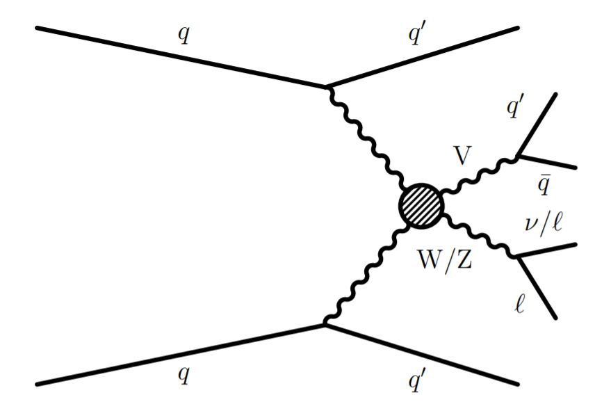
Figure 10: Feynman diagrams that involve triple and quadruple gauge couplings in proton-proton collisions [28].

The diagrams contributing to this process are shown in Fig. 10. We return again to the convention in which the Higgs doublet is represented as a vector with two complex components (see Eq. (3)), and the Skyrme term as a linear combination of the operators $Q_{\phi^{4}}^{(1)}$, $Q_{\phi^{4}}^{(2)}$ and $Q_{\phi^{4}}^{(3)}$. Their most general orthogonal linear combination is commonly denoted as

$$\begin{split}\mathcal{L}_{\phi^{4}}=&\ \frac{f_{S,0}}{M^{4}}Q_{\phi^{4}}^{(2)}+\frac{f_{S,1}}{M^{4}}Q_{\phi^{4}}^{(3)}+\frac{f_{S,2}}{M^{4}}Q_{\phi^{4}}^{(1)}\\ =&\ \frac{\alpha}{M^{4}}\mathcal{O}_{Sk}+\frac{\beta}{M^{4}}\cdot\frac{1}{2}\left[Q_{\phi^{4}}^{(2)}-Q_{\phi^{4}}^{(1)}\right]+\frac{\gamma}{M^{4}}\cdot\frac{1}{2}\left[Q_{\phi^{4}}^{(1)}+Q_{\phi^{4}}^{(2)}+Q_{\phi^{4}}^{(3)}\right],\end{split}$$ (89)

where $M$ is some mass scale. The three dimensionless coefficients $\alpha$, $\beta$ and $\gamma$ are linear functions of $f_{S,0}$, $f_{S,1}$ and $f_{S,2}$

$$\alpha=\frac{f_{S,0}+f_{S,2}-2f_{S,1}}{3}\ ,\qquad\beta=f_{S,0}-f_{S,2}\ ,\qquad\gamma=\frac{2}{3}(f_{S,0}+f_{S,1}+f_{S,2})\ .$$ (90)

By definition, the constant $\Lambda$ that multiplies $\mathcal{O}_{Sk}$ in the SMEFT expansion is

$$\frac{1}{\Lambda^{4}}=\frac{1}{3}\left(\frac{f_{S,0}}{M^{4}}+\frac{f_{S,2}}{M^{4}}-\frac{2f_{S,1}}{M^{4}}\right)\ .$$ (91)

The current upper bounds on $f_{S,0}$, $f_{S,1}$ and $f_{S,2}$ can be used to find a corresponding lower bound on $\Lambda$. The data for $f_{S,0}$ and $f_{S,1}$ from Ref. [28], with $95\%$ CL, are shown in the table below:

	$WW\ ({\rm TeV}^{-4})$	$WZ\ ({\rm TeV}^{-4})$
$f_{S,0}/M^{4}$	$[-2.7,2.7]$	$[-40,40]$
$f_{S,1}/M^{4}$	$[-3.3,3.4]$	$[-32,32]$

However, to the best of our knowledge, there are no data concerning $f_{S,2}$, nor any theoretical bound from e.g. unitarity or positivity that allow to express it as a function of $f_{S,0}$ and $f_{S,1}$. This makes constraining $\Lambda$ an impossible task.

In order to make sense of this data, we are forced to make some additional assumptions that cannot be justified from first principles. For example, we can assume that custodial symmetry is satisfied also to this order in the SMEFT, which is equivalent to imposing the constraint $f_{S,0}=f_{S,2}$. In this case

$$\frac{1}{\Lambda^{4}}=\frac{2}{3}\left(\frac{f_{S,0}}{M^{4}}-\frac{f_{S,1}}{M^{4}}\right)\quad\implies\quad\Lambda\gtrsim 0.71\ {\rm TeV}\ .$$ (92)

Another possibility is to fix the ratios between the $f_{S,i}$ using a UV completion of the Skyrme term. In Ref. [8], three different UV completions are given. The Skyrme term can be generated by an $SU(2)$ triplet vector boson $V^{\mu}_{a}$ with Lagrangian

$$\mathcal{L}_{\rm UV}=\frac{1}{2}\left(D_{\mu}V_{\nu}^{a}D^{\nu}V^{a\mu}-D_{\mu}V_{\nu}^{a}D^{\mu}V^{a\nu}+M^{2}V_{\mu}^{a}V^{a\mu}\right)+g_{V}V_{\mu}^{a}2\ \mathrm{Im}\left(\phi^{\dagger}\sigma^{a}D^{\mu}\phi\right)\ .$$ (93)

Computing the Wilson coefficients, one can show that

$$f_{S,0}=f_{S,2}=-\frac{1}{2}f_{S,1}\quad\implies\quad\Lambda\gtrsim 0.74\ {\rm TeV}\ .$$ (94)

Another possibility is to generate the Skyrme term through a scalar singlet $S$ with Lagrangian

$$\mathcal{L}_{\rm UV}=-\frac{1}{2}S(D^{2}+M^{2})S+\kappa_{S}S|\phi|^{2}\ .$$ (95)

In this case

$$f_{S,2}=f_{S,0}=0\quad\implies\quad\Lambda\gtrsim 0.82\ {\rm TeV}\ .$$ (96)

In general, due to the fact in Eq. (92) there is the fourth power of $\Lambda$, for any model that predicts ratios $\alpha/f_{S,j}\sim\mathcal{O}(1)$ the corresponding bound for $\Lambda$ is very close to $0.7-0.8\ {\rm TeV}$, except when $f_{S,0}+f_{S,2}-2f_{S,1}$ is very close to zero.

6.2 Dark matter

In this section we compute the relic abundance of cosmological EWSs. We assume that:

1. The cosmological EWSs have been produced after the electroweak phase transition ($T_{\rm EW}\simeq 10^{15}K$). This assumption is necessary, as the classical solution does not exist in the unbroken phase of the theory.

2. The production was thermal i.e. the EWSs, $S$, have been produced in reactions of the form $X+\bar{X}\to S+\bar{S}$ where $X$ are Standard Model particles. These reactions, of course, conserve $B+L$. As we are neglecting those production channels that result in a net $B+L$ change, we are probably misestimating the abundance actually predicted by the model.

3. The cosmological EWSs freeze out at $T\sim M/30$, and at that moment were non-relativistic.

4. The thermally averaged cross section of the EWSs can be roughly approximated by the geometric cross section $\expectationvalue{\sigma v}\sim\pi\lambda_{\text{Compton}}^{2}$ at $\Lambda\simeq 130$ (see Sec. 2.4).

Given these assumptions, we can compute the abundance with the solution of the Boltzmann equation [29, 30]:

$$\Omega_{S}h^{2}\sim 0.1\left(\frac{x_{f}}{10}\right)\left(\frac{10}{g_{*}(M)}\right)^{1/2}\frac{10^{-8}\mathrm{GeV}^{-1}}{\expectationvalue{\sigma v}}\ ,$$ (97)

where $x_{f}=M/T\sim 30$ at freeze out and $g_{*}(M)\sim 90$ is the number of relativistic degrees of freedom at temperature $M$. The results of this calculations is

$$\Omega_{S}h^{2}\sim 10^{-5}\ ,$$ (98)

which is significantly smaller than the DM abundance $\Omega_{DM}h^{2}\simeq 0.2$. It is instructive to compare our results with those of Ref. [8]. Assuming the $\Lambda$-dependence of the EWS mass and radius to be that in Eq. (27) and applying the formula (97), one obtains $\Omega_{S}h^{2}\simeq(\Lambda/3\ \mathrm{TeV})^{4}$, which, at the classical-to-quantum transition $\Lambda\simeq 310\ \mathrm{GeV}$ is approximately $\Omega_{S}h^{2}\sim 10^{-4}$. We conclude that thermally produced EWSs cannot be considered plausible DM candidates.

7 Conclusion

In this paper we discussed various aspects of the electroweak-Skyrme theory. This model has been studied in the past, always with the assumption of the Higgs field frozen at the vacuum expectation value. Recently, this model has been reconsidered assuming a dynamical Higgs field. Our finding is that the effect of the dynamical Higgs is even greater than previously recognized. We find that in the range of $\Lambda$ from $100$ to $300$ GeV, the EWS mass goes from $350$ to $30$ GeV, roughly a factor 10 lower than what was previously found. The profile functions for the EWS show two regions: one internal where the Higgs field is vanishing and the gauge fields are at their maximum value, and one external with no gauge fields and where the Higgs approaches its vacuum expectation value. As $\Lambda$ is increased the soliton becomes smaller and lighter, as expected before. We considered the rotational degrees of freedom and their quantization. We found that in the region of parameters we are considering, the gap in the rotational energies is of order of GeV, thus considerably smaller than the EWS mass scale. The rotational energy gap is big enough to justify the rigid rotor approximation we have been using. We showed that, if no other terms are present in the effective Lagrangian, the EWS must be quantized as a boson and the ground state is a scalar particle with spin zero. For the vibrational energy scales, we considered the breather (interpreted as a particle, it is often called an oscillon), a particular vibration of the scale factor which is relatively easy to compute, and should give the right order of magnitude of the vibrational scales.

We considered the effect of the hypercharge, as a perturbation of the EWS. This gives a magnetic dipole moment to the classical EWS. When the rotational degrees of freedom are quantized, the magnetic dipole is oriented toward the spin direction of the particle. In the spin-zero ground state, there is no remnant of the magnetic dipole moment. We considered fermion interactions with the electroweak Skyrmion. They can induce a fermion number to the EWS through the Goldstone-Wilczek mechanism. We considered the coupling of the EWS with the vector bosons and the Higgs field, and then computed the large distance interaction potential between two solitons.

We then consider, at the qualitative level, the issues of stability and quantum corrections. The EWS is not a topologically protected soliton, it is separated by the sphaleron barrier to the normal vacuum. It is, at most, metastable. In the region of parameters we considered, with $\Lambda$ above $100$ GeV. The mass of the EWS is always well below the sphaleron barrier, so for any phenomenologically reasonable value of $\Lambda$ we expect to have a metastable soliton. Quantum corrections are expected to be very important. At $\Lambda\simeq 200$ GeV the EWS is already at the scale of the Higgs mass. In general, solitons can be treated semi-classically only if they are heavier than any perturbative particle. So we can trust a semiclassical soliton analysis in a relatively small window, between the stability barrier $\Lambda_{\rm min}$ (which we can estimate roughly to be 50 GeV) and the region where quantum effects become considerable $\Lambda_{\rm max}$ (which we can estimate to be roughly 200 GeV). For larger values of $\Lambda$, the particle corresponding to the EWS is certainly there, and it is metastable with a very large lifetime. We cannot say much about its properties such as mass, radius and coupling with other particles. A naive extrapolation of the semiclassical analysis would predict that the mass goes to zero as $\Lambda\to\infty$, but a conservative guess is that it will stabilize itself around the Higgs mass scale.

Phenomenological constraints on $\Lambda$ are quite severe, and they impose a parameter space that is outside the rigorous validity of the approximations we have made. For $\Lambda$ in the range preferred by phenomenology, the EWS is a very quantum soliton and also very stable. This poses an interesting challenge for the future as this particle should be there, at least for this choice of higher-derivative corrections, and it is not semiclassical. Another aspect to look into is the modification of the EWS sector as we change the types of higher-derivative corrections.

Various things remain to be explored in the future. One aspect that should be considered with more precision is a complete analysis of the energy functional in the landscape of field configurations, with the sphaleron and all the possible saddle points, and how they are affected by the combination of Higgs mass and Skyrme term. To study the exact decay process, one should look, at least semiclassically, at the bounce solution to understand precisely the tunneling process that leads to the EWS decay. The numerical approach, both for the landscape and for the bounce problems, is quite complex to be carried out with the same precision we obtained for the solution of the EWS and this would require dedicated work in the future. Another task for future work is to study multi-EWS bound states. The multi-Skyrmions are very well studied in the Skyrme literature, and are known to be very stable solutions with multiple baryon numbers. They should also exist in the electroweak Skyrme model and may have an impact on the phenomenological aspects. From a phenomenological perspective, the most pressing thing to do now would be to learn how to treat the EWS in a region of parameter space where quantum corrections are large.

Acknowledgments

We thank Paolo Panci for useful discussions, especially on the phenomenological aspects of this problem. We also thank Alfredo Urbano and Antonio Junior Iovino for useful discussions. Finally, we thank the anonymous referee for questions on the stability of the EWS. The work of S. B. is supported by the INFN special project grant “GAST”. S. B. G. thanks the Outstanding Talent Program of Henan University and the Ministry of Education of Henan Province for partial support. The work of S. B. G. is supported by the National Natural Science Foundation of China (Grants No. 11675223 and No. 12071111) and by the Ministry of Science and Technology of China (Grant No. G2022026021L). The work of G. S. is supported by the INFN special project grant “GAGRA”.

Appendix A The breather

The scaling law under dilatations of the EWS fields are expressed in Eq. (48), and the new time-component of the weak gauge field is introduced in Eq. (50). We plug these transformed quantities into the Lagrangian and find an effective action for the dilatation parameter $\eta$. The terms that do not depend on $W_{0}$ can be easily found by a change of variables. Define

$$A \equiv\int{\mathrm{d}}^{3}x\left(\frac{1}{4g^{2}}\mathrm{tr}\ W_{ij}^{2}-\frac{1}{8\Lambda^{4}}\mathrm{tr}(D_{i}\Phi^{\dagger}D_{j}\Phi-D_{j}\Phi^{\dagger}D_{i}\Phi)^{2}\right),$$ (99a)

$$B \equiv\int{\mathrm{d}}^{3}x\ \frac{1}{2}\mathrm{tr}\ D_{i}\Phi^{\dagger}D_{i}\Phi,$$ (99b)

$$C \equiv\int{\mathrm{d}}^{3}x\ \frac{\lambda}{4}(\mathrm{tr}\ \Phi^{\dagger}\Phi-v^{2})^{2}\ ,$$ (99c)

then

$$A\longmapsto\eta A\ ,\qquad B\longmapsto\frac{B}{\eta}\ ,\qquad C\longmapsto\frac{C}{\eta^{3}}\ .$$ (100)

The virial law for the static solution reads

$$A=B+3C\ .$$ (101)

The remaining terms are the time-dependent terms:

$$\frac{1}{2}D_{1}\frac{\dot{\eta}^{2}}{\eta^{3}} \equiv\frac{1}{2}\int d^{3}x\ W_{0i}^{a}W_{0i}^{a}-\frac{1}{8\Lambda^{2}}\int d^{3}x\ 2\tr(D_{[0}\Phi^{\dagger}D_{i]}\Phi)^{2}\ ,$$ (102a)

$$\frac{1}{2}D_{2}\frac{\dot{\eta}^{2}}{\eta^{5}} \equiv\frac{1}{2}\int d^{3}x\;\tr D_{0}\Phi^{\dagger}D_{0}\Phi\ .$$ (102b)

We now make the rescaling

$$r\to\frac{v}{\Lambda^{2}}r\ ,\qquad t\to\frac{v}{\Lambda^{2}}t\ ,\qquad(f_{1},f_{2},b,\xi)\to\frac{2}{g}(f_{1},f_{2},b,\xi)\ .$$ (103)

We introduce the dimensionless Lagrangian for the breather

$$L_{\text{br,nat}}=\frac{1}{2}\left(D_{1,\rm nat}+\frac{D_{2,\rm nat}}{\eta^{2}}\right)\frac{\dot{\eta}^{2}}{\eta^{3}}-\left(\eta A_{\text{nat}}+\frac{1}{\eta}B_{\text{nat}}+\frac{1}{\eta^{3}}C_{\text{nat}}\right)\ ,$$ (104)

where the dimensionless coefficients obey

$$(L_{\text{br}},A,B,C,D_{1},D_{2})=\frac{4\pi v^{3}}{\Lambda^{2}}(L_{\text{br,nat}},A_{\text{nat}},B_{\text{nat}},C_{\text{nat}},D_{1,\rm nat},D_{2,\rm nat})\ ,$$ (105)

and are given by

$$A_{\text{nat}} =\int_{0}^{\infty}{\mathrm{d}}r\bigg{\{}\alpha\left[\left(f_{1}^{\prime}-2f_{2}\frac{b}{r}\right)^{2}+\left(f_{2}^{\prime}+(2f_{1}-1)\frac{b}{r}\right)^{2}+\frac{2}{r^{2}}\left(f_{1}^{2}+f_{2}^{2}-f_{1}\right)^{2}\right]$$

$$\phantom{=\int_{0}^{\infty}{\mathrm{d}}r\bigg{\{}\ }+(f_{1}^{2}+f_{2}^{2})\sigma^{2}\left[(\sigma^{\prime})^{2}+\frac{\sigma^{2}}{r^{2}}\left(b^{2}+\frac{f_{1}^{2}+f_{2}^{2}}{2}\right)\right]\bigg{\}}\ ,$$ (106a)

$$B_{\text{nat}} =\int_{0}^{\infty}{\mathrm{d}}r\left[\frac{r^{2}}{2}(\sigma^{\prime})^{2}+\sigma^{2}\left(f_{1}^{2}+f_{2}^{2}+\frac{b^{2}}{2}\right)\right]\ ,$$ (106b)

$$C_{\text{nat}} =\int_{0}^{\infty}{\mathrm{d}}r\beta r^{2}(\sigma^{2}-1)^{2}\ ,$$ (106c)

$$D_{1,\rm nat} =\int_{0}^{\infty}r^{2}{\mathrm{d}}r\bigg{\{}2\alpha\left[\left(f_{1}^{\prime}-\frac{2\xi f_{2}}{r}\right)^{2}+\left(f_{2}^{\prime}-\xi\frac{1-2f_{1}}{r}\right)^{2}+\frac{1}{2}(b^{\prime}-\xi^{\prime})^{2}\right]$$

$$\phantom{=\int_{0}^{\infty}r^{2}{\mathrm{d}}r\bigg{\{}\ }+2\sigma^{2}\left[(f_{1}^{2}+f_{2}^{2})\left((\sigma^{\prime})^{2}+\frac{\xi^{2}\sigma^{2}}{r^{2}}\right)+\frac{(\sigma^{\prime})^{2}}{2}(\xi-b)^{2}\right]\bigg{\}}\ ,$$ (106d)

$$D_{2,\rm nat} =\int_{0}^{\infty}r^{2}{\mathrm{d}}r\left(r^{2}(\sigma^{\prime})^{2}+\xi^{2}\sigma^{2}\right)\ .$$ (106e)

$\alpha$ and $\beta$ are defined in Eq. (30). For small perturbations $\epsilon=\eta-1$ around the classical minimum, the Lagrangian reduces to that of a harmonic oscillator with frequency

$$\omega_{c}=\sqrt{\frac{2B_{\text{nat}}+12C_{\text{nat}}}{D_{1,\rm nat}+D_{2,\rm nat}}}\ .$$ (107)

The new profile function $\xi$ can be determined as a function of $f_{1}$, $f_{2}$, $b$ and $\sigma$. If we consider $\xi$ as a dynamical variable of the system, it must satisfy the Euler-Lagrange equation

$$\left(\frac{{\mathrm{d}}}{{\mathrm{d}}r}\frac{\delta}{\delta\xi^{\prime}}-\frac{\delta}{\delta\xi}\right)L_{\text{br,nat}}=0\quad\implies\quad\left(\frac{{\mathrm{d}}}{{\mathrm{d}}r}\frac{\delta}{\delta\xi^{\prime}}-\frac{\delta}{\delta\xi}\right)(D_{1,\rm nat}+D_{2,\rm nat})=0\ .$$ (108)

Suitable boundary conditions are

$$\xi(0)=0\ ,\qquad\xi(\infty)=0\ .$$ (109)

Explicitly, the equation of motion for $\xi$ is

$$\begin{split}\xi^{\prime\prime}-b^{\prime\prime}+\frac{2}{r}(\xi^{\prime}-b^{\prime})&=-\left(f_{1}^{\prime}-\frac{2\xi f_{2}}{r}\right)\frac{4f_{2}}{r}+\left(f_{2}^{\prime}-\xi\frac{1-2f_{1}}{r}\right)\frac{2(2f_{1}-1)}{r}\\ &\phantom{=\ }+\frac{\sigma^{2}}{\alpha}\left[\xi+\frac{2\xi\sigma^{2}(f_{1}^{2}+f_{2}^{2})}{r^{2}}+(\sigma^{\prime})^{2}(\xi-b)\right]\ .\end{split}$$ (110)

An educated guess is that the solution of $\xi$ is $\xi=b$, since this reduces the equation of motion to an algebraic equation that can easily be compared to that for $b$. We obtain

$$-\left(f_{1}^{\prime}-\frac{2bf_{2}}{r}\right)\frac{4f_{2}}{r}+\left(f_{2}^{\prime}-b\frac{1-2f_{1}}{r}\right)\frac{2(2f_{1}-1)}{r}+\frac{\sigma^{2}}{\alpha}\left[b+\frac{2b\sigma^{2}(f_{1}^{2}+f_{2}^{2})}{r^{2}}\right]=0\ ,$$ (111)

which can be solved for $b$:

$$b=\frac{2r\alpha(2f_{2}f_{1}^{\prime}+(1-2f_{1})f_{2}^{\prime})}{2\alpha\left((1-2f_{1})^{2}+4f_{2}^{2}\right)+r^{2}\sigma^{2}+2(f_{1}^{2}+f_{2}^{2})\sigma^{4}}\ ,$$ (112)

which is exactly the static equation of motion for $b$. This establishes that $\xi=b$ is a solution. A quick inspection of Eqs. (106)-(106e) shows that $\xi=b$ is a local minimum of $D_{1,\rm nat}+D_{2,\rm nat}$, and thus it maximizes $\omega_{c}$.

Appendix B Interaction potentials

In this appendix, we briefly show how to compute the interaction potential between two solitons taking into account all the relevant contributions. In order to avoid irrelevant complications, we consider the case of a soliton made of a scalar field $\phi$ with action

$$S(\phi)=\int{\mathrm{d}}^{4}x\left[\frac{1}{2}\partial_{\mu}\phi\ \partial^{\mu}\phi-\frac{1}{2}m^{2}\phi^{2}+V(\phi)\right]\ .$$ (113)

Let $\phi(\textbf{x})$ be a soliton field configuration. For $|\textbf{x}|\gg R$, with $R$ being the soliton radius, the asymptotic field $\phi_{\infty}(\textbf{x})$ satisfies the approximate equations of motion

$$(-\nabla^{2}+m^{2})\phi_{\infty}(\textbf{x})=S(\textbf{x})\ ,$$ (114)

where $S(\textbf{x})$ is a source with support in $\textbf{x}=0$. Let $\phi(\textbf{x}-\textbf{x}_{1})$ and $\phi(\textbf{x}-\textbf{x}_{2})$ be two identical solitons with $\textbf{x}_{12}\gg R$. Far from $\textbf{x}_{1}$ and $\textbf{x}_{2}$, the total asymptotic field $\phi_{\infty}(\textbf{x})=\phi_{\infty}(\textbf{x}-\textbf{x}_{1})+\phi_{\infty}(\textbf{x}-\textbf{x}_{2})$ satisfies

$$(-\nabla^{2}+m^{2})\phi_{\infty}(\textbf{x})=S(\textbf{x}-\textbf{x}_{1})+S(\textbf{x}-\textbf{x}_{2})\ .$$ (115)

From these equations of motion, and neglecting anharmonic contributions, we can guess an approximate expression for the total energy of the two solitons

$$E_{\mathrm{tot}}=2E_{\mathrm{sol}}+\int d^{3}\textbf{x}\left[\phi^{(1)}(-\nabla^{2}+m^{2})\phi^{(2)}-\phi^{(2)}S^{(1)}-\phi^{(1)}S^{(2)}\right]+\ldots$$ (116)

where we have used the notation $\phi^{(i)}=\phi_{\infty}(\textbf{x}-\textbf{x}_{i})$ and $S^{(i)}=S(\textbf{x}-\textbf{x}_{i})$ and where $E_{\mathrm{sol}}$ is the energy of a single soliton. The ellipses contain anharmonic terms, that can be neglected within our approximation. The first term of the integrand in Eq. (116) yields the tail-tail contributions, while the other two terms yield the core-tail contribution. Using the equations of motion, one ends up with

$$E_{\mathrm{tot}}=2E_{\mathrm{sol}}-\int d^{3}\textbf{x}\ \phi^{(1)}(-\nabla^{2}+m^{2})\phi^{(2)}+\ldots$$ (117)

which explains the minus sign in Eq. (81). The resulting interaction potential is always attractive, in agreement with the particle exchange interpretation.

Appendix C Asymptotic behavior of the EWS fields

C.1 Fields at large distance

The asymptotic behavior of the solutions can be easily found by inserting the Ansatz (80) into the linearized equations of motion. The results obtained with this method depend only on the quadratic part of the action and on the form of the Ansatz

$$\left(-\nabla^{2}+m_{h}^{2}\right)\Phi(\textbf{x})=0\ ,\qquad\left(-\nabla^{2}+m_{W}^{2}\right)W_{i}(\textbf{x})=0\ ,\qquad\partial_{i}W_{i}(\textbf{x})=0\ .$$ (118)

The linearized equations (118) must be valid for $\textbf{x}\neq 0$. As shown in App. B their right-hand side can contain a distribution with support at the origin. Solving the linearized equations for the Higgs field, we simply obtain

$$\sigma(r)\underset{r\to\infty}{\longrightarrow}1+\frac{c_{h}}{m_{h}}\frac{e^{-m_{h}r}}{4\pi r}\ ,\qquad\sigma(r)\underset{r\to 0}{\longrightarrow}d_{h}\frac{e^{m_{h}r}-e^{-m_{h}r}}{m_{h}r}\ ,$$ (119)

where $c_{h}$ and $d_{h}$ are real constants. For the weak gauge fields, the linearized equations of motion for the functions $F_{1}=\frac{f_{1}}{r}$, $F_{2}=\frac{f_{2}}{r}$ and $B=\frac{b}{r}$ are coupled

$$\hat{x}_{a}\left[B^{\prime}+\frac{2}{r}(B-F_{2})\right]=0\ ,$$ (120a)

$$\begin{split}\varepsilon_{aij}\hat{x}_{j}\left[F_{1}^{\prime\prime}+\frac{2}{r}F_{1}^{\prime}-\frac{2}{r^{2}}F_{1}-m_{W}^{2}F_{1}\right]+\hat{x}_{i}\hat{x}_{a}\left[B^{\prime\prime}+\frac{2}{r}B^{\prime}-\frac{4}{r^{2}}(B-F_{2})-m_{W}^{2}B\right]\\ \mathop{+}(\delta_{ia}-\hat{x}_{i}\hat{x}_{a})\left[F_{2}^{\prime\prime}+\frac{2}{r}F_{2}^{\prime}+\frac{2}{r^{2}}(B-F_{2})-m_{W}^{2}F_{2}\right]=0\ .\end{split}$$ (120b)

The independence of the three members of the second equation can be easily proven by multiplying them by $\hat{x}_{i}$, $(\delta_{ik}-\hat{x}_{i}\hat{x}_{k})$ and $\varepsilon_{aik}\hat{x}_{k}$. The first equation is a constraint on the initial conditions, so it introduces no redundancy in the system. The most general solution of these equations at infinity is

$$\begin{split}F_{1}(r)&\underset{r\to\infty}{\longrightarrow}\frac{c_{\alpha}}{4\pi}\left[j_{-2}(\mathrm{i}m_{W}r)+\mathrm{i}y_{-2}(\mathrm{i}m_{W}r)\right]\ ,\\ B(r)+2F_{2}(r)&\underset{r\to\infty}{\longrightarrow}\frac{c_{\beta}}{4\pi}\frac{e^{-m_{W}r}}{m_{W}r}\ ,\\ B(r)-F_{2}(r)&\underset{r\to\infty}{\longrightarrow}-\mathrm{i}\frac{c_{\gamma}}{4\pi}\left[j_{-3}(\mathrm{i}m_{W}r)+\mathrm{i}y_{-3}(\mathrm{i}m_{W}r)\right]\ ,\end{split}$$ (121)

where $c_{\alpha}$, $c_{\beta}$, $c_{\gamma}$ are real constants and $j_{\ell}$ and $y_{\ell}$ are spherical Bessel functions. Instead, for $r\rightarrow 0$, we have

$$\begin{split}F_{1}(r)&\underset{r\to 0}{\longrightarrow}\mathrm{i}d_{\alpha}\,y_{-2}(\mathrm{i}m_{W}r)\ ,\\ B(r)+2F_{2}(r)&\underset{r\to 0}{\longrightarrow}d_{\beta}\frac{e^{m_{W}r}-e^{-m_{W}r}}{m_{W}r}\ ,\\ B(r)-F_{2}(r)&\underset{r\to 0}{\longrightarrow}d_{\gamma}\,y_{-3}(\mathrm{i}m_{W}r)\ ,\end{split}$$ (122)

where $d_{\alpha}$, $d_{\beta}$, $d_{\gamma}$ are real constants. The constraint (120a) has not been imposed yet. This will be done in the next subsection by passing to momentum space.

C.2 Source terms

The source term for the Higgs field $h=v(\sigma-1)$ can be easily obtained from the distributional identity $(-\nabla^{2}+m^{2})\frac{e^{-mr}}{4\pi r}=\delta^{(3)}(\textbf{x})$ applied to the field in Eq. (119). The result is

$$S^{(h)}(\textbf{x})=\frac{c_{h}v}{m_{h}}\delta^{(3)}(\textbf{x})\ .$$ (123)

We now search for a source term for the weak fields $S^{(W)}$ satisfying

$$\left(-\nabla^{2}\delta_{ij}+\partial_{i}\partial_{j}+m_{W}^{2}\delta_{ij}\right)W_{j}(\textbf{x})=S^{(W)}_{i}(\textbf{x})\ .$$ (124)

The source $S^{(W)}_{i}$ can be a function of the derivatives $\partial_{i}$ and of the Pauli matrices $\tau^{a}$ applied on a Dirac delta centered at the origin, $\delta^{(3)}(\textbf{x})$, and must satisfy all the symmetries of $W_{i}$. In order to find the source, we make the Fourier transform of both sides of Eq. (124) using the same notation of Eq. (34). First, we rearrange the terms in Eq. (20) as

$$W_{ai}=\varepsilon_{aij}\hat{x}_{j}F_{1}+\left(\hat{x}_{i}\hat{x}_{a}-\frac{1}{3}\delta_{ia}\right)(B-F_{2})+\frac{1}{3}\delta_{ia}(B+2F_{2})\ .$$ (125)

Then, we separate the radial and angular part of the Fourier-transformed weak field by means of the identity

$$e^{-\mathrm{i}\textbf{p}\cdot\textbf{x}}=\sum_{\ell}(2\ell+1)(-\mathrm{i})^{\ell}P_{\ell}(\hat{p}\cdot\hat{x})j_{\ell}(pr)\ ,$$ (126)

where $P_{\ell}$ are the Legendre polynomials and $j_{\ell}$ are the modified spherical Bessel functions. For the angular part, we use the identities

$$\int{\mathrm{d}}\Omega_{\textbf{x}}P_{\ell}(\hat{x}\cdot\hat{p})=4\pi\delta_{\ell,0}\ ,$$ (127a)

$$\int{\mathrm{d}}\Omega_{\textbf{x}}\hat{x}_{i}P_{\ell}(\hat{x}\cdot\hat{p})=\frac{4\pi}{3}\delta_{\ell,1}\hat{p}_{i}\ ,$$ (127b)

$$\int{\mathrm{d}}\Omega_{\textbf{x}}\left(\hat{x}_{i}\hat{x}_{j}-\frac{1}{3}\delta_{ij}\right)P_{\ell}(\hat{x}\cdot\hat{p})=\frac{4\pi}{5}\delta_{\ell,2}\left(\hat{p}_{i}\hat{p}_{j}-\frac{1}{3}\delta_{ij}\right)\ .$$ (127c)

We find that

$$\widetilde{W}_{ai}(\textbf{p})= -4\pi\mathrm{i}\varepsilon_{aij}\hat{p}_{j}\int_{0}^{\infty}r^{2}{\mathrm{d}}r\ F_{1}(r)j_{1}(pr)+\frac{4\pi}{3}\delta_{ia}\int_{0}^{\infty}r^{2}{\mathrm{d}}r\ (B(r)+2F_{2}(r))j_{0}(pr)$$

$$-4\pi\left(\hat{p}_{i}\hat{p}_{j}-\frac{1}{3}\delta_{ij}\right)\int_{0}^{\infty}r^{2}{\mathrm{d}}r\ (B(r)-F_{2}(r))j_{2}(pr)\ .$$ (128)

Then we substitute the asymptotic expressions for $F_{1}$, $F_{2}$ and $B$ into the equation and use the integrals

$$\int_{0}^{\infty}r^{2}{\mathrm{d}}r\ \frac{e^{-ar}}{ar}j_{0}(qr)=\frac{1}{a}\frac{1}{q^{2}+a^{2}}\ ,$$ (129a)

$$\int_{0}^{\infty}r^{2}{\mathrm{d}}r\ \left(j_{-2}(\mathrm{i}ar)+\mathrm{i}y_{-2}(\mathrm{i}ar)\right)j_{1}(qr)=\frac{q}{a^{2}}\frac{1}{q^{2}+a^{2}}\ ,$$ (129b)

$$\int_{0}^{\infty}r{\mathrm{d}}r\ \left(j_{-3}(\mathrm{i}ar)+\mathrm{i}y_{-3}(\mathrm{i}ar)\right)j_{2}(qr)=\frac{\mathrm{i}q^{2}}{a^{3}}\frac{1}{q^{2}+a^{2}}\ .$$ (129c)

We finally obtain the result

$$\begin{split}\widetilde{W}_{ai}(\textbf{p})=-\frac{1}{p^{2}+m_{W}^{2}}\left[\mathrm{i}\frac{c_{\alpha}}{m_{W}^{2}}\varepsilon_{aij}p_{j}-\frac{1}{3}\delta_{ia}\frac{c_{\beta}}{m_{W}}+\left(p_{i}p_{a}-\frac{1}{3}\delta_{ia}p^{2}\right)\frac{c_{\gamma}}{m_{W}^{3}}\right]\ .\end{split}$$ (130)

Before applying the operator $(p^{2}\delta_{ij}-p_{i}p_{j}+m_{W}^{2}\delta_{ij})$, we need to impose the condition $\partial_{i}W_{i}^{a}(\textbf{x})=0$, which, in momentum space, takes the form

$$0=p_{i}\widetilde{W}_{ai}(\textbf{p})=\frac{1}{p^{2}+m_{W}^{2}}\left[\frac{1}{3}\frac{c_{\beta}}{m_{W}}-\frac{2c_{\gamma}}{3m_{W}^{3}}p^{2}\right]p_{a}\quad\implies\quad c_{\beta}=c_{\gamma}=0\ ,$$ (131)

which means that the source is

$$\widetilde{S}_{ai}^{(W)}(\textbf{p}) =-\mathrm{i}\frac{c_{\alpha}}{m_{W}^{2}}\varepsilon_{aij}p_{j}\ ,\qquad\text{(momentum space)}$$ (132a)

$$S_{ai}^{(W)}(\textbf{x}) =-\frac{c_{\alpha}}{m_{W}^{2}}\varepsilon_{aij}\partial_{j}\delta^{(3)}(\textbf{x})\ .\qquad\text{(position space)}$$ (132b)

The asymptotic expression for $W_{ai}$ in position space is thus

$$W_{ai}(\textbf{x})=-\frac{c_{\alpha}}{m_{W}^{2}}\varepsilon_{aij}\partial_{j}\frac{e^{-m_{W}r}}{4\pi r}\ .$$ (133)

References

- [1] T. H. R. Skyrme, A Nonlinear field theory, Proc. Roy. Soc. Lond. A 260 (1961) 127–138.
- [2] G. S. Adkins, C. R. Nappi, and E. Witten, Static Properties of Nucleons in the Skyrme Model, Nucl. Phys. B 228 (1983) 552.
- [3] E. D’Hoker and E. Farhi, Skyrmions And/in the Weak Interactions, Nucl. Phys. B 241 (1984) 109–128.
- [4] G. Eilam, D. Klabucar, and A. Stern, Skyrmion Solutions to the Weinberg-Salam Model, Phys. Rev. Lett. 56 (1986) 1331.
- [5] J. Ambjorn and V. A. Rubakov, Classical Versus Semiclassical Electroweak Decay of a Techniskyrmion, Nucl. Phys. B 256 (1985) 434–448.
- [6] Y. Brihaye and J. Kunz, Multi - Skyrmion Solutions in the Weinberg-Salam and Sakurai Model, Z. Phys. C 41 (1989) 663–666.
- [7] E. Farhi, J. Goldstone, A. Lue, and K. Rajagopal, Collision induced decays of electroweak solitons: Fermion number violation with two and few initial particles, Phys. Rev. D 54 (1996) 5336–5360, [hep-ph/9511219].
- [8] J. C. Criado, V. V. Khoze, and M. Spannowsky, The Emergence of Electroweak Skyrmions through Higgs Bosons, JHEP 03 (2021) 162, [arXiv:2012.07694].
- [9] J. Ellis, M. Karliner, and M. Praszalowicz, Generalized Skyrmions in QCD and the Electroweak Sector, JHEP 03 (2013) 163, [arXiv:1209.6430].
- [10] R. Kitano and M. Kurachi, Electroweak-Skyrmion as Topological Dark Matter, JHEP 07 (2016) 037, [arXiv:1605.07355].
- [11] R. Kitano and M. Kurachi, More on Electroweak-Skyrmion, JHEP 04 (2017) 150, [arXiv:1703.06397].
- [12] Y. Hamada, R. Kitano, and M. Kurachi, Electroweak-Skyrmion as asymmetric dark matter, JHEP 02 (2022) 124, [arXiv:2108.12185].
- [13] J. C. Criado, V. V. Khoze, and M. Spannowsky, Electroweak skyrmions in the HEFT, JHEP 12 (2021) 026, [arXiv:2109.01596].
- [14] F. R. Klinkhamer and N. S. Manton, A Saddle Point Solution in the Weinberg-Salam Theory, Phys. Rev. D 30 (1984) 2212.
- [15] T. Cohen, N. Craig, X. Lu, and D. Sutherland, Is SMEFT Enough?, JHEP 03 (2021) 237, [arXiv:2008.08597].
- [16] C. W. Murphy, Dimension-8 operators in the Standard Model Eective Field Theory, JHEP 10 (2020) 174, [arXiv:2005.00059].
- [17] E. D’Hoker and E. Farhi, Decoupling a Fermion in the Standard Electroweak Theory, Nucl. Phys. B 248 (1984) 77.
- [18] E. D’Hoker and E. Farhi, Decoupling a Fermion Whose Mass Is Generated by a Yukawa Coupling: The General Case, Nucl. Phys. B 248 (1984) 59–76.
- [19] S. Das Bakshi, J. Chakrabortty, C. Englert, M. Spannowsky, and P. Stylianou, violation at ATLAS in effective field theory, Phys. Rev. D 103 (2021), no. 5 055008, [arXiv:2009.13394].
- [20] N. S. Manton and P. Sutcliffe, Topological solitons. Cambridge Monographs on Mathematical Physics. Cambridge University Press, 2004.
- [21] V. A. Rubakov, B. E. Stern, and P. G. Tinyakov, On the electroweak decay of a technibaryon in the soliton model, Phys. Lett. B 160 (1985) 292–296.
- [22] G. S. Adkins and C. R. Nappi, The Skyrme Model with Pion Masses, Nucl. Phys. B 233 (1984) 109–115.
- [23] H. Weigel, Chiral Soliton Models for Baryons, vol. 743. Springer, 2008.
- [24] N. S. Manton, Topology in the Weinberg-Salam Theory, Phys. Rev. D 28 (1983) 2019.
- [25] J. Goldstone and R. Jackiw, Quantization of Nonlinear Waves, Phys. Rev. D 11 (1975) 1486–1498.
- [26] I. J. R. Aitchison and C. M. Fraser, Derivative Expansions of Fermion Determinants: Anomaly Induced Vertices, Goldstone-Wilczek Currents and Skyrme Terms, Phys. Rev. D 31 (1985) 2605.
- [27] N. H. Christ, Conservation Law Violation at High-Energy by Anomalies, Phys. Rev. D 21 (1980) 1591.
- [28] CMS Collaboration, A. M. Sirunyan et al., Search for anomalous electroweak production of vector boson pairs in association with two jets in proton-proton collisions at 13 TeV, Phys. Lett. B 798 (2019) 134985, [arXiv:1905.07445].
- [29] E. W. Kolb and M. S. Turner, The Early Universe, vol. 69. Westview Press, 1990.
- [30] D. Baumann, Cosmology. Cambridge University Press, 7, 2022.