Abstract

In this paper, we extend the spectral method developed [10] to any dimension $d\geqslant 1$, in order to construct an eigen-solution for the Fokker-Planck operator with heavy tail equilibria, of the form $(1+|v|^{2})^{-\frac{\beta}{2}}$, in the range $\beta\in]d,d+4[$. The method developed in dimension 1 was inspired by the work of H. Koch on nonlinear KdV equation [19]. The strategy in this paper is the same as in dimension 1 but the tools are different, since dimension 1 was based on ODE methods. As a direct consequence of our construction, we obtain the fractional diffusion limit for the kinetic Fokker-Planck equation, for the correct density $\rho:=\int_{\mathbb{R}^{d}}f\mathrm{d}v$, with a fractional Laplacian $\kappa(-\Delta)^{\frac{\beta-d+2}{6}}$ and a positive diffusion coefficient $\kappa$.

1 Introduction

1.1 Setting of the problem

In this present paper, we deal with the kinetic Fokker-Planck (FP) equation, which describes in a deterministic way the Brownian motion of a set of particles. It is given by the following form

$$\left\{\begin{array}[]{l}\partial_{t}f+v\cdot\nabla_{x}f=Q(f),\;\;\;t\geqslant 0,\ x\in\mathbb{R}^{d},\ v\in\mathbb{R}^{d},\\ \\ f(0,x,v)=f_{0}(x,v),\;\;\quad x\in\mathbb{R}^{d},\ v\in\mathbb{R}^{d},\end{array}\right.$$ (1.1)

where the collisional Fokker-Planck operator $Q$ is given by

$$Q(f)=\nabla_{v}\cdot\bigg{(}F\nabla_{v}\bigg{(}\frac{f}{F}\bigg{)}\bigg{)},$$ (1.2)

and $F$ is the equilibrium of $Q$, a fixed function which depends only on $v$ and satisfying

$$Q(F)=0\quad\mbox{ and }\quad\int_{\mathbb{R}^{d}}F(v)\ \mathrm{d}v=1.$$

Provided $f_{0}\geqslant 0$, the unknown $f(t,x,v)\geqslant 0$ can be interpreted as the density of particles occupying at time $t\geqslant 0$, the position $x\in\mathbb{R}^{d}$ with velocity $v\in\mathbb{R}^{d}$.

Recall that one of the motivations for studying the classical or fractional diffusion limit is to simplify the equations for some collisional kinetic models when the interaction between particles are the dominant phenomena and when the observation time is very large. For that purpose, we introduce a small parameter, $\varepsilon\ll 1$, the mean free path and we proceed to rescaling the distribution function $f(t,x,v)$ in time and space

$$t=\frac{t^{\prime}}{\theta(\varepsilon)}\quad\mbox{ and }\quad x=\frac{x^{\prime}}{\varepsilon}\quad\mbox{ with }\quad\theta(\varepsilon)\underset{\varepsilon\to 0}{\longrightarrow}0,$$

which leads to the following rescaled equation (without primes)

$$\left\{\begin{array}[]{l}\theta(\varepsilon)\partial_{t}f^{\varepsilon}+\varepsilon v\cdot\nabla_{x}f^{\varepsilon}=Q(f^{\varepsilon}),\;\;\;t\geqslant 0,x\in\mathbb{R}^{d},v\in\mathbb{R}^{d},\\ \\ f^{\varepsilon}(0,x,v)=f_{0}(x,v),\;\;\;\;x\in\mathbb{R}^{d},v\in\mathbb{R}^{d}.\end{array}\right.$$ (1.3)

Note that initial condition written in non rescaled variable are well prepared conditions.

The goal is then to study the behavior of the solution $f^{\varepsilon}$ as $\varepsilon\to 0$. Formally, passing to the limit when $\varepsilon\to 0$ in the equation (1.3), we obtain that the limit $f^{0}$ is in the kernel of $Q$ which is spanned by the equilibrium $F$, which means that $f^{0}=\rho(t,x)F(v)$. Thus, it amounts to find the equation satisfied by the density $\rho$. Note that this limit depends on the nature of the equilibrium $F$ considered as well as on the chosen change of time scale $\theta(\varepsilon)$.

For Gaussian equilibria, it is classical (see [2],[4],[12],[20],[11] for Boltzmann and [13] for Fokker Planck) that by taking the classical time scaling $\theta(\varepsilon)=\varepsilon^{2}$, we obtain a diffusion equation

$$\partial_{t}\rho-\nabla_{x}\cdot(D\nabla_{x}\rho)=0,$$ (1.4)

where

$$D=\int vQ^{-1}(-vF)\mathrm{d}v.$$ (1.5)

For slowly decreasing equilibria, or so-called heavy tail equilibria of the form $F(v)\sim\langle v\rangle^{-\beta}$, it is more complicated, and this study has been the interest of many papers in the last few years, with different methods and for different collision operators. Fractional diffusion limit has been obtained in the case of the linear Boltzmann equation when the cross section is such that the operator has a spectral gap, see [23] for the pioneer paper in the case of space independent cross section, where the authors used a method based on Fourier-Laplace transformation, and see [22] for a weak convergence result obtained by the Moment method, which also applies to cross sections that depend on the position variable. See also [24] for a probabilistic approach.

In the present work, we consider for any $\beta>d$, heavy tail equilibria

$$F(v)=\frac{C_{\beta}^{2}}{(1+|v|^{2})^{\frac{\beta}{2}}},$$

where $C_{\beta}$ is a normalization constant.

The diffusion limit for the FP equation seems more complicated then the linear Boltzmann one, and the main difficulty is due to the fact that the Fokker-Planck operator $Q$ has no spectral gap. In addition, for this equation, all the terms of the operator participate in the limit, i.e. the collision and advection parts. In [25], the classical scaling is studied and it is proved in any dimension $d$ that we obtain a diffusion equation (1.4), with diffusion coefficient (1.5) as soon as $\beta>d+4$. The critical case where $\beta=d+4$ is studied in [9], where the expected result of classical diffusion with an anomalous time scaling is proved, $\theta(\varepsilon)=\varepsilon^{2}|{\rm log}\varepsilon|$. A unified presentation of the result for even more general cases of $\beta$ can be found in recent papers where the result has been obtained, by probabilistic method in [15] and [14], and using a weighted density in [7]. In this last paper, in addition to the diffusion limit results, an estimates on the fluid approximation error have been obtained. We refer also to [6] for this last point, where the authors have developed an $L^{2}$-hypocoercivity approach and established an optimal decay rate, determined by a fractional Nash type inequality, compatible with the fractional diffusion limit.

The aim of this paper is to study the case $d<\beta<d+4$. By taking as test function the eigenvector of the whole Fokker-Planck operator (advection $+$ collisions), which converges towards equilibrium $F$, we capture at the limit the “diffusion” equation for any $\beta>d$. The computation of the eigenvalue gives us the right scaling in time, $\theta(\varepsilon)$, and the diffusion coefficient $\kappa$ at the same time. We are therefore interested in a new problem: the construction of an eigen-solution for the whole Fokker-Planck operator, which is the main subject of this paper.

The diffusion limit for the FP equation has already been obtained recently in dimension 1 [21] with a spectral method, based on the reconnection of two branches on $\mathbb{R}_{+}$ and $\mathbb{R}_{-}$, but this method of reconnection is difficult to adapt in dimension $d$. This led us to look for another strategy, which was the subject of [10], a method inspired by the work of H. Koch on nonlinear KdV equation [19], which allowed us to construct an eigen-solution for the spectral problem associated to the whole Fokker-Planck operator with ODE methods in dimension 1. The aim of this paper is to develop PDE methods in order to obtain the result in any dimension. This method is interesting since it can be used for different potentials like convolution, or for nonlinear equations as well. Moreover, as in dimension 1, a splitting of the Fokker-Planck operator is involved, which recalls the enlargement theory for nonlinear Boltzmann operator when there are spectral gap issues. This theory was developed by Gualdani, Mischler and Mouhot in [17] whose key idea was based on the decomposition of the operator into two parts, a dissipative part plus a regularizing part. See also [16] and references therein.

1.2 Setting of the result

Before stating our main result, let us give some notations that we will use along this paper.

Notations. As in [21], in order to simplify the computation and work with a self-adjoint operator in $L^{2}$, we proceed to a change of unknown by writing

$$f=F^{\frac{1}{2}}g=C_{\beta}Mg$$

with

$$M:=C_{\beta}^{-1}F^{\frac{1}{2}}=\frac{1}{(1+|v|^{2})^{\frac{\gamma}{2}}},$$

since we impose $\gamma:=\frac{\beta}{2}>\frac{d}{2}$, $F\in L^{1}(\mathbb{R}^{d})$ then, $M\in L^{2}(\mathbb{R}^{d})$ and $C_{\beta}$ is chosen such that

$$\int_{\mathbb{R}^{d}}F\mathrm{d}v=1.$$

The equation (1.3) becomes

$$\theta(\varepsilon)\partial_{t}g^{\varepsilon}+\varepsilon v\cdot\nabla_{x}g^{\varepsilon}=\frac{1}{M}\nabla_{v}\cdot\bigg{(}M^{2}\nabla_{v}\bigg{(}\frac{g^{\varepsilon}}{M}\bigg{)}\bigg{)}=\Delta_{v}g^{\varepsilon}-W(v)g^{\varepsilon},$$

with

$$W(v)=\frac{\Delta_{v}M}{M}=\frac{\gamma(\gamma-d+2)|v|^{2}-\gamma d}{(1+|v|^{2})^{2}}.$$

We see the equation as

$$\theta(\varepsilon)\partial_{t}g^{\varepsilon}=-\mathcal{L}_{\varepsilon}g^{\varepsilon},$$

where

$$\mathcal{L}_{\varepsilon}:=-\Delta_{v}+W(v)+\varepsilon v\cdot\nabla_{x}=-(Q-\varepsilon v\cdot\nabla_{x})$$

and

$$Q:=-\Delta_{v}+W(v).$$

We operate a Fourier transform in $x$ and since the operator $Q$ has coefficient that do not depend on $x$, we get:

$$\theta(\varepsilon)\partial_{t}\hat{g}^{\varepsilon}=-\mathcal{L}_{\eta}\hat{g}^{\varepsilon},$$ (1.6)

where

$$\mathcal{L}_{\eta}:=-\Delta_{v}+W(v)+\mathrm{i}\eta v_{1}$$

with

$$\eta:=\varepsilon|\xi|\quad\mbox{ and }\quad v_{1}:=v\cdot\frac{\xi}{|\xi|},$$

where $\xi$ being the space Fourier variable.

The operator $\mathcal{L}_{\eta}$ is an unbounded self-adjoint operator acting on $L^{2}$. Its domain is given by

$$D(\mathcal{L}_{\eta})=\big{\{}g\in L^{2}(\mathbb{R}^{d})\ ;\ \Delta_{v}g\in L^{2}(\mathbb{R}^{d}),v_{1}g\in L^{2}(\mathbb{R}^{d})\big{\}}.$$

Main results.

Theorem 1.1 (Eigen-solution for the Fokker-Planck operator)

Assume that $d<\beta<d+4$ with $\beta\neq d+1$. Let $\eta_{0}>0$ and $\lambda_{0}>0$ small enough. Then, for all $\eta\in[0,\eta_{0}]$, there exists a unique eigen-couple $\big{(}\mu(\eta),M_{\eta}\big{)}$ in $\{\mu\in\mathbb{C},|\mu|\leqslant\eta^{\frac{2}{3}}\lambda_{0}\}\times L^{2}(\mathbb{R}^{d},\mathbb{C})$, solution to the spectral problem

$$\mathcal{L}_{\eta}(M_{\mu,\eta})(v)=\big{[}-\Delta_{v}+W(v)+\mathrm{i}\eta v_{1}\big{]}M_{\mu,\eta}(v)=\mu M_{\mu,\eta}(v),\ v\in\mathbb{R}^{d}.$$ (1.7)

Moreover,
1. The following convergence in the Sobolev space $H^{1}(\mathbb{R}^{d})$ holds:

$$\big{\|}M_{\eta}-M\big{\|}_{H^{1}(\mathbb{R}^{d})}\underset{\eta\to 0}{\longrightarrow}0.$$ (1.8)

2. The eigenvalue $\mu(\eta)$ is given by

$$\mu(\eta)={\overline{\mu}}(-\eta)=\kappa|\eta|^{\frac{\beta-d+2}{3}}\big{(}1+O(|\eta|^{\frac{\beta-d+2}{3}})\big{)},$$ (1.9)

where $\kappa$ is a positive constant given by

$$\kappa=-2C_{\beta}^{2}\int_{\{s_{1}>0\}}s_{1}|s|^{-\gamma}\mbox{Im}H_{0}(s)\mathrm{d}s,$$ (1.10)

and where $H_{0}$ is the unique solution to the equation

$$\big{[}-\Delta_{s}+\frac{\gamma(\gamma-d+2)}{|s|^{2}}+\mathrm{i}s_{1}\big{]}H_{0}(s)=0,\quad\forall s\in\mathbb{R}^{d}\setminus\{0\},$$ (1.11)

satisfying

$$\int_{\{|s_{1}|\geqslant 1\}}|H_{0}(s)|^{2}\mathrm{d}s<\infty\quad\mbox{ and }\quad H_{0}(s)\underset{0}{\sim}|s|^{-\gamma}.$$ (1.12)

Introduce $V$, the space defined by

$$V:=\left\{f:\mathbb{R}^{d}\rightarrow\mathbb{R},\int_{\mathbb{R}^{d}}\frac{|f|^{2}}{F}\ \mathrm{d}v<\infty\mbox{ and }\int_{\mathbb{R}^{d}}\bigg{|}\nabla_{v}\bigg{(}\frac{f}{F}\bigg{)}\bigg{|}^{2}F\mathrm{d}v<\infty\right\},$$

$V^{\prime}$ being its dual, and

$$Y:=\left\{f\in L^{2}\big{(}[0,T]\times\mathbb{R}^{d};V\big{)};\ \theta(\varepsilon)\partial_{t}f+\varepsilon v\cdot\nabla_{x}f\in L^{2}\big{(}[0,T]\times\mathbb{R}^{d};V^{\prime}\big{)}\right\}.$$

Theorem 1.2 (Fractional diffusion limit for the Fokker-Planck equation)

Assume that $d<\beta<d+4$ with $\beta\neq d+1$. Assume that $f_{0}\in L^{1}(\mathbb{R}^{2d})$ is a non-negative function in $L^{2}_{F^{-1}}(\mathbb{R}^{2d})\cap L^{\infty}_{F^{-1}}(\mathbb{R}^{2d})$. Let $f^{\varepsilon}$ be the solution of (1.3) in $Y$ with initial data $f_{0}$, with $\theta(\varepsilon)=\varepsilon^{\frac{\beta-d+2}{3}}$. Let $\kappa$ be the constant given by (1.10).
Then $f^{\varepsilon}$ converges weakly star in $L^{\infty}\big{(}[0,T],\ L^{2}_{F^{-1}}(\mathbb{R}^{2d})\big{)}$ towards $\rho(t,x)F(v)$ where $\rho(t,x)$ is the solution to

$$\partial_{t}\rho+\kappa(-\Delta)^{\frac{\beta-d+2}{6}}\rho=0,\quad\rho(0,x)=\int_{\mathbb{R}^{d}}f_{0}\mathrm{d}v.$$ (1.13)

Remark 1.3

The hypothesis $\beta\neq d+1$ is technical. It avoids to introduce logarithmic terms in the expression of $\mu(\eta)$.

Ideas of the proof and outline of the paper.

The proof of Theorem 1.1 is done in two main steps, both based on the Implicit Function Theorem (IFT). First, we consider what we call a penalized equation, given by

$$\left\{\begin{array}[]{l}\big{[}-\Delta_{v}+W(v)+\mathrm{i}\eta v_{1}\big{]}M_{\mu,\eta}(v)=\mu M_{\mu,\eta}(v)-\langle M_{\mu,\eta}-M,\Phi\rangle\Phi(v),\ v\in\mathbb{R}^{d},\\ \\ M_{\mu,\eta}\in L^{2}(\mathbb{R}^{d}).\end{array}\right.$$ (1.14)

where $\Phi$ is a function, that satisfies some assumptions, that we will determine later. The additional term allows us to avoid the problem of reconnection by ensuring existence of a solution to equation (1.14) on the whole space $\mathbb{R}^{d}$ for any $\eta$ and $\mu$. This is one of the key points of this method. Also, note that the sign before the scalar product $\langle M_{\mu,\eta}-M,\Phi\rangle$ is important.

The aim of the first step is to show the existence of a unique solution for equation (1.14) for $\eta$ and $\mu$ fixed, which is the purpose of Section 2. As we said above, we will decompose the operator $``-\Delta_{v}+W(v)+\mathrm{i}\eta v_{1}-\mu"$ in two parts. The first one is chosen such that it admits an inverse that is continuous as a linear operator between two suitable functional spaces, continuous with respect to the parameters $\eta$ and $\mu$ and compact at $\eta=\mu=0$. The second part of the operator is left in the right-hand side of the equation, i.e. is considered as a source term. The invertibility of the first part is the subject of the first subsection, and it is based on an elaborated version of the Lax-Milgram theorem. While the study of the inverse operator and its properties is the subject of the second subsection whose main result is the existence of solutions for equation (1.14).

In the second step, to ensure that the additional term vanishes, we have to chose $\mu(\eta)$ obtained via the Implicit Function Theorem around the point $(\mu,\eta)=(0,0)$. The study of this constraint is the subject of a large part of section 3 which is composed of three subsections. The first one is dedicated to the $L^{2}$ estimates for the solution of the penalized equation (1.14). It consists in improving the space to which the solution found by Lax-Milgram belongs. It is the objective of the second subsection. The last subsection is dedicated to the approximation of the eigenvalue and the computation of the diffusion coefficient.

The last section is devoted to the proof of Theorem 1.2. It consists of two subsections, a priori estimates and limiting process in the weak formulation of equation (1.6).

2 Existence of solutions for the penalized equation

We start this section by some notations and definition of the considered operators. Let $\mu=\lambda\eta^{\frac{2}{3}}$ with $\lambda\in\mathbb{C}$ and let denote by $L_{\lambda,\eta}$ the operator

$$L_{\lambda,\eta}:=-\Delta_{v}+\tilde{W}(v)+\mathrm{i}\eta v_{1}-\lambda\eta^{\frac{2}{3}},$$

where

$$\tilde{W}(v):=\frac{\gamma(\gamma-d+2)}{1+|v|^{2}}.$$

Let denote by $V:=\tilde{W}-W$. We have

$$V(v)=\frac{\gamma(\gamma+2)}{(1+|v|^{2})^{2}}.$$

We will rewrite the equation (1.14) as follows

$$\left\{\begin{array}[]{l}L_{\lambda,\eta}(M_{\lambda,\eta})=V(v)M_{\lambda,\eta}-\langle M_{\lambda,\eta}-M,\Phi\rangle\Phi,\ v\in\mathbb{R}^{d},\\ \\ M_{\lambda,\eta}\in L^{2}(\mathbb{R}^{d}).\end{array}\right.$$ (2.1)

The two equations (1.14) and (2.1) are equivalent.

Remark 2.1

1. Since $L_{\lambda,0}$ does not depend on $\lambda$, let’s denote it by $L_{0}$, $L_{0}:=L_{\lambda,0}$.

2. If $\ {\overline{\Phi}}(-v)=\Phi(v)$ and $M_{\lambda,\eta}(v_{1},v^{\prime})$ satisfies the equation (2.1), then $\overline{M}_{{\overline{\lambda}},\eta}(-v_{1},v^{\prime})$ satisfies also (2.1), since the potential $W$ is symmetric for a symmetric equilibrium $M$. Note that this is where the symmetry of the equilibrium $M$ is used and therefore this is a “non-drift condition”.

3. Note that the splitting of the potential $W$ into $\tilde{W}$ and $V$ is crucial in our study. It plays a very important role whether in the invertibility of the operator $L_{\lambda,\eta}$ or in the compactness of its inverse at the point $(\lambda,\eta)=(0,0)$.

2.1 Coercivity and Lax-Milgram theorem

The purpose of this subsection is to show that the operator $L_{\lambda,\eta}$ defined above is invertible. For this, we are going to define a Hilbert space $\mathcal{H}_{\eta}$ as well as a scalar product $\langle\cdot,\cdot\rangle_{\mathcal{H}_{\eta}}$ on which we apply a Lax-Milgram theorem.

Definition 2.2

$\bullet$ We define the Hilbert space $\mathcal{H}_{\eta}$ as being the completion of the space $C_{c}^{\infty}(\mathbb{R}^{d},\mathbb{C})$ for the norm $\|\cdot\|_{\mathcal{H}_{\eta}}$ induced from the scalar product $\langle\cdot,\cdot\rangle_{\mathcal{H}_{\eta}}$

$$\mathcal{H}_{\eta}:=\overline{\big{\{}\psi\in C_{c}^{\infty}(\mathbb{R}^{d},\mathbb{C});\ \|\psi\|_{\tilde{\mathcal{H}}_{\eta}}^{2}:=\langle\psi,\psi\rangle_{\tilde{\mathcal{H}}_{\eta}}<+\infty\big{\}}},$$

where

$$\langle\psi,\phi\rangle_{\tilde{\mathcal{H}}_{\eta}}:=\int_{\mathbb{R}^{d}}\nabla_{v}\bigg{(}\frac{\psi}{M}\bigg{)}\cdot\nabla_{v}\bigg{(}\frac{{\overline{\phi}}}{M}\bigg{)}\ M^{2}\mathrm{d}v+\int_{\mathbb{R}^{d}}V\psi{\overline{\phi}}\ \mathrm{d}v+\eta\int_{\mathbb{R}^{d}}|v_{1}|\psi{\overline{\phi}}\ \mathrm{d}v,$$

and where $\ V(v):=\tilde{W}(v)-W(v)=\frac{\gamma(\gamma+2)}{(1+|v|^{2})^{2}}>0\$ for all $\ v\in\mathbb{R}^{d}$.

We have the embeddings

$$\mathcal{H}_{\eta}\subseteq\mathcal{H}_{\eta^{*}}\subseteq\mathcal{H}_{0},\quad\forall\ 0\leqslant\eta^{*}\leqslant\eta$$

since $\ \|\cdot\|_{\tilde{\mathcal{H}}_{0}}\leqslant\|\cdot\|_{\tilde{\mathcal{H}}_{\eta^{*}}}\leqslant\|\cdot\|_{\tilde{\mathcal{H}}_{\eta}}\$ for all $\ 0\leqslant\eta^{*}\leqslant\eta$.

$\bullet$ We define the sesquilinear form $a$ on $\mathcal{H}_{\eta}\times\mathcal{H}_{\eta}$ by

$$a(\psi,\phi):=\int_{\mathbb{R}^{d}}\nabla_{v}\bigg{(}\frac{\psi}{M}\bigg{)}\cdot\nabla_{v}\bigg{(}\frac{{\overline{\phi}}}{M}\bigg{)}\ M^{2}\mathrm{d}v+\int_{\mathbb{R}^{d}}V\psi{\overline{\phi}}\ \mathrm{d}v+\mathrm{i}\eta\int_{\mathbb{R}^{d}}v_{1}\psi{\overline{\phi}}\ \mathrm{d}v-\lambda\eta^{\frac{2}{3}}\int_{\mathbb{R}^{d}}\psi{\overline{\phi}}\ \mathrm{d}v.$$

Remark 2.3

1. Note that $a(\psi,\psi)\neq\|\psi\|_{\tilde{\mathcal{H}}_{\eta}}$.

2. Note that the sesquilinear form $a$ depends on $\lambda$ and $\eta$ and in order to simplify the notation, we omit the subscript when no confusion is possible.

3. Let us denote by $\tilde{Q}$ the operator $\tilde{Q}:=-\Delta_{v}+\tilde{W}(v)$. We have $\tilde{Q}=Q+V$. Thus, the operator $\tilde{Q}$ is dissipative since

   $$\int_{\mathbb{R}^{d}}\tilde{Q}(\psi)\psi\ \mathrm{d}v=\int_{\mathbb{R}^{d}}Q(\psi)\psi\ \mathrm{d}v+\int_{\mathbb{R}^{d}}V|\psi|^{2}\ \mathrm{d}v=\int_{\mathbb{R}^{d}}\bigg{|}\nabla_{v}\bigg{(}\frac{\psi}{M}\bigg{)}\bigg{|}^{2}M^{2}+V|\psi|^{2}\ \mathrm{d}v\geqslant 0.$$

   Note that we have also the equality

   $$\int_{\mathbb{R}^{d}}\tilde{Q}(\psi)\psi\ \mathrm{d}v=\int_{\mathbb{R}^{d}}\big{|}\nabla_{v}\psi\big{|}^{2}\ \mathrm{d}v+c_{\gamma,d}\int_{\mathbb{R}^{d}}\frac{|\psi|^{2}}{\langle v\rangle^{2}}\ \mathrm{d}v,$$

   with $\ c_{\gamma,d}:=\gamma(\gamma-d+2)$. Observe that $\ c_{\gamma,d}<0\$ for $\ \gamma\in(\frac{d}{2},\frac{d+4}{2})\$ with $\ d>4$.

4. Since $\ \tilde{Q}=Q+V\$ then, the sesquilinear form $a$ can be written as follows:

   $$a(\psi,\phi)=\int_{\mathbb{R}^{d}}\nabla_{v}\psi\cdot\nabla_{v}{\overline{\phi}}\ \mathrm{d}v+c_{\gamma,d}\int_{\mathbb{R}^{d}}\frac{\psi{\overline{\phi}}}{\langle v\rangle^{2}}\ \mathrm{d}v+\mathrm{i}\eta\int_{\mathbb{R}^{d}}v_{1}\psi{\overline{\phi}}\ \mathrm{d}v-\lambda\eta^{\frac{2}{3}}\int_{\mathbb{R}^{d}}\psi{\overline{\phi}}\ \mathrm{d}v.$$

Lemma 2.4

The norm defined by

$$\|\psi\|_{{\mathcal{H}}_{\eta}}^{2}:=\int_{\mathbb{R}^{d}}\big{|}\nabla_{v}\psi\big{|}^{2}\ \mathrm{d}v+\int_{\mathbb{R}^{d}}\frac{|\psi|^{2}}{\langle v\rangle^{2}}\ \mathrm{d}v+\eta\int_{\mathbb{R}^{d}}|v_{1}||\psi|^{2}\ \mathrm{d}v$$

is induced from the scalar product

$$\langle\psi,\phi\rangle_{{\mathcal{H}}_{\eta}}:=\int_{\mathbb{R}^{d}}\nabla_{v}\psi\cdot\nabla_{v}{\overline{\phi}}\ \mathrm{d}v+\int_{\mathbb{R}^{d}}\frac{\psi{\overline{\phi}}}{\langle v\rangle^{2}}\ \mathrm{d}v+\eta\int_{\mathbb{R}^{d}}|v_{1}|\psi{\overline{\phi}}\ \mathrm{d}v,$$

and the two norms $\|\cdot\|_{\mathcal{H}_{\eta}}$ and $\|\cdot\|_{\tilde{\mathcal{H}}_{\eta}}$ are equivalent, i.e., there are two positive constants $C_{1}$ and $C_{2}$ such that

$$C_{1}\|\psi\|_{\tilde{\mathcal{H}}_{\eta}}\leqslant\|\psi\|_{{\mathcal{H}}_{\eta}}\leqslant C_{2}\|\psi\|_{\tilde{\mathcal{H}}_{\eta}},\quad\forall\psi\in\mathcal{H}_{\eta}.$$

To prove this Lemma, we need the Hardy-Poincaré inequality that we recall in the following

Lemma 2.5 (Hardy-Poincaré inequality)

[5] Let $d\geqslant 1$ and $\alpha_{*}=\frac{2-d}{2}$. For any $\alpha<0$, and $\alpha\in(-\infty,0)\setminus\{\alpha_{*}\}$ for $d\geqslant 3$, there is a positive constant $\Lambda_{\alpha,d}$ such that

$$\Lambda_{\alpha,d}\int_{\mathbb{R}^{d}}|f|^{2}(D+|x|^{2})^{\alpha-1}\mathrm{d}x\leqslant\int_{\mathbb{R}^{d}}|\nabla f|^{2}(D+|x|^{2})^{\alpha}\mathrm{d}x$$ (2.2)

holds for any function $f\in H^{1}\big{(}(D+|x|^{2})^{\alpha}\mathrm{d}x\big{)}$ and any $D\geqslant 0$, under the additional condition $\int_{\mathbb{R}^{d}}f(D+|x|^{2})^{\alpha-1}\mathrm{d}x=0$ and $D>0$ if $\alpha<\alpha_{*}$.

Remark 2.6

For $\displaystyle f=\frac{g}{M}$, $D=1$ and $\alpha=-\gamma$ in the previous lemma, the inequality becomes

$$\Lambda_{\alpha,d}\int_{\mathbb{R}^{d}}\frac{|g|^{2}}{\langle v\rangle^{2}}\mathrm{d}v\leqslant\int_{\mathbb{R}^{d}}\bigg{|}\nabla_{v}\bigg{(}\frac{g}{M}\bigg{)}\bigg{|}^{2}M^{2}\ \mathrm{d}v,$$ (2.3)

and the orthogonality condition becomes

$$\int_{\mathbb{R}^{d}}\frac{gM}{\langle v\rangle^{2}}\mathrm{d}v=0$$ (2.4)

since $\ -\gamma<\frac{2-d}{2}=:\alpha_{*}\$ for $\ \gamma\in(\frac{d}{2},\frac{d+4}{2})$.
If we denote by

$$\mathcal{P}(g):=\left(\int_{\mathbb{R}^{d}}\frac{M^{2}}{\langle v\rangle^{2}}\mathrm{d}v\right)^{-1}\int_{\mathbb{R}^{d}}\frac{gM}{\langle v\rangle^{2}}\mathrm{d}v.$$

Then, the inequality (2.3) can be written for all $g\in\mathcal{H}_{0}$

$$\Lambda_{\alpha,d}\int_{\mathbb{R}^{d}}\frac{\big{|}g-\mathcal{P}(g)M\big{|}^{2}}{\langle v\rangle^{2}}\mathrm{d}v\leqslant\int_{\mathbb{R}^{d}}\bigg{|}\nabla_{v}\bigg{(}\frac{g}{M}\bigg{)}\bigg{|}^{2}M^{2}\ \mathrm{d}v.$$ (2.5)

Proof of Lemma 2.4. Let’s start with the right inequality: $\|\psi\|_{{\mathcal{H}}_{\eta}}\leqslant C_{2}\|\psi\|_{\tilde{\mathcal{H}}_{\eta}}$. Let $\psi\in\mathcal{H}_{\eta}$. Then, since $M\in L^{2}(\mathbb{R}^{d})$, by Cauchy-Schwarz inequality we get

$$\bigg{|}\int_{\mathbb{R}^{d}}\frac{\psi M}{\langle v\rangle^{2}}\mathrm{d}v\bigg{|}\leqslant\left(\int_{\mathbb{R}^{d}}\frac{|\psi|^{2}}{\langle v\rangle^{4}}\mathrm{d}v\right)^{\frac{1}{2}}\left(\int_{\mathbb{R}^{d}}M^{2}\mathrm{d}v\right)^{\frac{1}{2}}\leqslant\frac{1}{\gamma(\gamma+2)}\|\psi\|_{\tilde{\mathcal{H}}_{\eta}}.$$

Now, since the function $\psi-\mathcal{P}(\psi)M$ satisfies the condition (2.4), $\mathcal{P}\big{(}\psi-\mathcal{P}(\psi)M\big{)}=0$, then the inequality (2.3) can be used and therefore

$$\int_{\mathbb{R}^{d}}\frac{|\psi|^{2}}{\langle v\rangle^{2}}\mathrm{d}v =\int_{\mathbb{R}^{d}}\frac{|\psi-\mathcal{P}(\psi)M+\mathcal{P}(\psi)M|^{2}}{\langle v\rangle^{2}}\mathrm{d}v$$

$$\leqslant 2\left(\Lambda_{\alpha,d}^{-1}\int_{\mathbb{R}^{d}}\bigg{|}\nabla_{v}\bigg{(}\frac{\psi}{M}\bigg{)}\bigg{|}^{2}M^{2}\ \mathrm{d}v+|\mathcal{P}(\psi)|^{2}\int_{\mathbb{R}^{d}}\frac{M^{2}}{\langle v\rangle^{2}}\mathrm{d}v\right)$$

$$\leqslant 2\left(\Lambda_{\alpha,d}^{-1}\|\psi\|_{\tilde{\mathcal{H}}_{\eta}}^{2}+\frac{1}{\gamma^{2}(\gamma+2)^{2}}\left(\int_{\mathbb{R}^{d}}\frac{M^{2}}{\langle v\rangle^{2}}\mathrm{d}v\right)^{-1}\|\psi\|_{\tilde{\mathcal{H}}_{\eta}}^{2}\right)$$

$$\leqslant C_{\gamma,d}\|\psi\|_{\tilde{\mathcal{H}}_{\eta}}^{2}.$$

We have by the first point of Remark 2.3

$$\int_{\mathbb{R}^{d}}\tilde{Q}(\psi)\psi\ \mathrm{d}v=\int_{\mathbb{R}^{d}}\bigg{|}\nabla_{v}\bigg{(}\frac{\psi}{M}\bigg{)}\bigg{|}^{2}M^{2}+V|\psi|^{2}\ \mathrm{d}v=\int_{\mathbb{R}^{d}}\big{|}\nabla_{v}\psi\big{|}^{2}\ \mathrm{d}v+c_{\gamma,d}\int_{\mathbb{R}^{d}}\frac{|\psi|^{2}}{\langle v\rangle^{2}}\ \mathrm{d}v.$$

From where we get

$$\int_{\mathbb{R}^{d}}\big{|}\nabla_{v}\psi\big{|}^{2}\ \mathrm{d}v\leqslant\int_{\mathbb{R}^{d}}\bigg{|}\nabla_{v}\bigg{(}\frac{\psi}{M}\bigg{)}\bigg{|}^{2}M^{2}+V|\psi|^{2}\ \mathrm{d}v+|c_{\gamma,d}|\int_{\mathbb{R}^{d}}\frac{|\psi|^{2}}{\langle v\rangle^{2}}\ \mathrm{d}v\leqslant\big{(}1+\tilde{C}_{\gamma,d}\big{)}\|\psi\|_{\tilde{\mathcal{H}}_{\eta}}^{2}.$$

Hence,

$$\|\psi\|_{{\mathcal{H}}_{\eta}}\leqslant C_{2}\|\psi\|_{\tilde{\mathcal{H}}_{\eta}},$$

with $C_{2}:=\sqrt{2(1+\tilde{C}_{\gamma,d})}$ a positive constant which depends only on $\gamma$ and $d$.
To get inequality $C_{1}\|\psi\|_{\tilde{\mathcal{H}}_{\eta}}\leqslant\|\psi\|_{{\mathcal{H}}_{\eta}}$, it is enough just to write

$$\int_{\mathbb{R}^{d}}\bigg{|}\nabla_{v}\bigg{(}\frac{\psi}{M}\bigg{)}\bigg{|}^{2}M^{2}+V|\psi|^{2}\ \mathrm{d}v=\int_{\mathbb{R}^{d}}\big{|}\nabla_{v}\psi\big{|}^{2}\ \mathrm{d}v+c_{\gamma,d}\int_{\mathbb{R}^{d}}\frac{|\psi|^{2}}{\langle v\rangle^{2}}\ \mathrm{d}v\leqslant(1+|c_{\gamma,d}|)\|\psi\|_{{\mathcal{H}}_{\eta}}^{2}.$$

Hence,

$$C_{1}\|\psi\|_{\tilde{\mathcal{H}}_{\eta}}\leqslant\|\psi\|_{{\mathcal{H}}_{\eta}},$$

with $C_{1}:=(2+|c_{\gamma,d}|)^{-\frac{1}{2}}$ a positive constant which depends only on $\gamma$ and $d$. $\square$

In the remainder of this section, we will work with the norm $\|\cdot\|_{{\mathcal{H}}_{\eta}}$.

Before moving on to the continuity of $a$, we will prove a Poincaré type inequality which we give in the following lemma:

Lemma 2.7

Let $\eta>0$ be fixed. Then, there exists a constant $C_{0}>0$, independent of $\eta$ such that the following inequality holds true

$$\|\psi\|_{L^{2}(\mathbb{R}^{d})}\leqslant C_{0}\eta^{-\frac{1}{3}}\|\psi\|_{\mathcal{H}_{\eta}},\quad\forall\psi\in\mathcal{H}_{\eta}.$$

Proof. We will split the integral of $\|\psi\|_{L^{2}(\mathbb{R}^{2})}^{2}$ into two parts $\{|v_{1}|\leqslant\eta^{-\frac{1}{3}}\}$ and $\{|v_{1}|\geqslant\eta^{-\frac{1}{3}}\}$.
$\bullet$ On $\{|v_{1}|\geqslant\eta^{-\frac{1}{3}}\}$, we simply have

$$\eta^{\frac{2}{3}}\int_{\{|v_{1}|\geqslant\eta^{-\frac{1}{3}}\}}|\psi|^{2}\mathrm{d}v\leqslant\int_{\{|v_{1}|\geqslant\eta^{-\frac{1}{3}}\}}\eta|v_{1}||\psi|^{2}\mathrm{d}v\leqslant\|\psi\|^{2}_{\mathcal{H}_{\eta}}.$$

$\bullet$ While on $\{|v_{1}|\leqslant\eta^{-\frac{1}{3}}\}$, we introduce the function $\zeta_{\eta}$ defined by: $\zeta_{\eta}(v_{1}):=\zeta\big{(}\eta^{\frac{1}{3}}v_{1})$, where $\zeta\in C^{\infty}(\mathbb{R})$ such that $0\leqslant\zeta\leqslant 1$, $\zeta\equiv 1$ on $B(0,1)$ and $\zeta\equiv 0$ outside of $B(0,2)$. Then, one has

$$\eta^{\frac{2}{3}}\int_{\{|v_{1}|\leqslant\eta^{-\frac{1}{3}}\}}|\psi|^{2}\mathrm{d}v \leqslant\eta^{\frac{2}{3}}\int_{\{|v_{1}|\leqslant 2\eta^{-\frac{1}{3}}\}}|\zeta_{\eta}\psi|^{2}\mathrm{d}v$$

$$=\eta^{\frac{2}{3}}\int_{\{|v_{1}|\leqslant 2\eta^{-\frac{1}{3}}\}}\bigg{|}\int\int_{-2\eta^{-\frac{1}{3}}}^{v_{1}}\partial_{w_{1}}(\zeta_{\eta}\psi)\mathrm{d}w_{1}\bigg{|}^{2}\mathrm{d}v^{\prime}\mathrm{d}v_{1}$$

$$\leqslant\eta^{\frac{2}{3}}\int_{\{|v_{1}|\leqslant 2\eta^{-\frac{1}{3}}\}}\bigg{(}\int_{-2\eta^{-\frac{1}{3}}}^{v_{1}}\mathrm{d}w_{1}\bigg{)}\bigg{(}\int_{-2\eta^{-\frac{1}{3}}}^{v_{1}}|\partial_{w_{1}}(\zeta_{\eta}\psi)|^{2}\mathrm{d}w_{1}\bigg{)}\mathrm{d}v$$

$$\leqslant 16\big{\|}\partial_{v_{1}}(\zeta_{\eta}\psi)\big{\|}^{2}_{L^{2}(\{|v_{1}|\leqslant 2\eta^{-\frac{1}{3}}\})}.$$

On the other hand, one has

$$\big{|}\partial_{v_{1}}(\zeta_{\eta}\psi)\big{|}^{2} =|\zeta_{\eta}^{\prime}\psi|^{2}+|\zeta_{\eta}\partial_{v_{1}}\psi|^{2}+\zeta_{\eta}\zeta_{\eta}^{\prime}\big{(}{\overline{\psi}}\partial_{v_{1}}\psi+\psi\overline{\partial_{v_{1}}\psi}\big{)}$$

$$\leqslant\big{(}\eta^{-1}|v_{1}|^{-1}|\zeta_{\eta}^{\prime}|^{2}\big{)}\eta|v_{1}||\psi|^{2}+|\partial_{v_{1}}\psi|^{2}+2\eta^{-\frac{1}{2}}|v_{1}|^{-\frac{1}{2}}|\zeta_{\eta}^{\prime}|\big{(}\eta^{\frac{1}{2}}|v_{1}|^{\frac{1}{2}}|\psi|\big{)}|\partial_{v_{1}}\psi|,$$

and since $\zeta_{\eta}^{\prime}=0$ except on $\{\eta^{-\frac{1}{3}}\leqslant|v_{1}|\leqslant 2\eta^{-\frac{1}{3}}\}$, where $|\eta^{-\frac{1}{2}}|v_{1}|^{-\frac{1}{2}}\zeta_{\eta}^{\prime}(v_{1})|\leqslant C$. Then, by integrating the last inequality and using Cauchy-Schwarz for the last term we get

$$\big{\|}\partial_{v_{1}}(\zeta_{\eta}\psi)\big{\|}^{2}_{L^{2}(\{|v_{1}|\leqslant 2\eta^{-\frac{1}{3}}\})} \lesssim\int_{\{|v_{1}|\geqslant\eta^{-\frac{1}{3}}\}}\eta|v_{1}||\psi|^{2}\mathrm{d}v+\|\partial_{v_{1}}\psi\|^{2}_{L^{2}(\{|v_{1}|\leqslant 2\eta^{-\frac{1}{3}}\})}\lesssim\|\psi\|^{2}_{\mathcal{H}_{\eta}}.$$

Note that we used the inclusion $\{\eta^{-\frac{1}{3}}\leqslant|v_{1}|\leqslant 2\eta^{-\frac{1}{3}}\}\subset\{|v_{1}|\geqslant\eta^{-\frac{1}{3}}\}$. Hence, the inequality of Lemma 2.7 holds. $\square$

Lemma 2.8

The sesquilinear form $a$ is continuous on $\mathcal{H}_{\eta}\times\mathcal{H}_{\eta}$. Moreover, there exists a constant $C>0$, independent of $\lambda$ and $\eta$ such that, for all $\psi,\phi\in\mathcal{H}_{\eta}$

$$|a(\psi,\phi)|\leqslant C\|\psi\|_{\mathcal{H}_{\eta}}\|\phi\|_{\mathcal{H}_{\eta}}.$$

Proof. It follows from the previous lemma that allows to handle the term $\displaystyle\eta^{\frac{2}{3}}\lambda\int\psi{\overline{\phi}}$ $\square$

Remark 2.9

By application of Riesz’s theorem to continuous sesquilinear forms, there exists a continuous linear map $A_{\lambda,\eta}\in\mathcal{L}({\mathcal{H}_{\eta}})$ such that $\ a(\psi,\phi)=\langle A_{\lambda,\eta}\psi,\phi\rangle_{\mathcal{H}_{\eta}}$ for all $\psi,\phi\in\mathcal{H}_{\eta}$.
Note that $A_{\lambda,\eta}$ depends on $\lambda$ and $\eta$ since the form $a$ depends on these last parameters.

Lemma 2.10

Let $\eta>0$ and $\lambda\in\mathbb{C}$ fixed, such that $|\lambda|\leqslant\lambda_{0}$ with $\lambda_{0}$ small enough. Let $A_{\lambda,\eta}$ be the linear operator representing the sesquilinear form $a$. Then, there exists a constant $C>0$, independent of $\lambda$ and $\eta$ such that

$$\|\psi\|_{\mathcal{H}_{\eta}}\leqslant C\|A_{\lambda,\eta}\psi\|_{\mathcal{H}_{\eta}},\quad\forall\psi\in\mathcal{H}_{\eta}.$$ (2.6)

Proof. We have for all $a,b\in\mathbb{R}$ and $z\in\mathbb{C}$: $|a+\mathrm{i}b+z|\geqslant|a|-|z|$. Now, applying this inequality to $|a(\psi,\psi)|$ and using the Lemma 2.7 for the term which contains $\lambda$, we write

$$|a(\psi,\psi)| =\bigg{|}\int_{\mathbb{R}^{d}}\big{(}|\nabla_{v}\psi|^{2}+c_{\gamma}\frac{|\psi|^{2}}{\langle v\rangle^{2}}+\mathrm{i}\eta v_{1}|\psi|^{2}-\lambda\eta^{\frac{2}{3}}|\psi|^{2}\big{)}\mathrm{d}v\bigg{|}$$

$$\geqslant\bigg{|}\int_{\mathbb{R}^{d}}\big{(}|\nabla_{v}\psi|^{2}+c_{\gamma}\frac{|\psi|^{2}}{\langle v\rangle^{2}}\big{)}\mathrm{d}v\bigg{|}-|\lambda|\eta^{\frac{2}{3}}\|\psi\|_{2}^{2}$$

$$\geqslant\|\psi\|^{2}_{\mathcal{H}_{0}}-C_{0}|\lambda|\|\psi\|^{2}_{\mathcal{H}_{\eta}}.$$

Then, since $|a(\psi,\psi)|=|\langle A_{\lambda,\eta}\psi,\psi\rangle_{\mathcal{H}_{\eta}}|\leqslant\|A_{\lambda,\eta}\psi\|_{\mathcal{H}_{\eta}}\|\psi\|_{\mathcal{H}_{\eta}}$, we get

$$\|\psi\|^{2}_{\mathcal{H}_{0}}=\|\nabla_{v}\psi\|^{2}_{2}+c_{\gamma}\bigg{\|}\frac{\psi}{\langle v\rangle}\bigg{\|}^{2}_{2}\leqslant\|A_{\lambda,\eta}\psi\|_{\mathcal{H}_{\eta}}\|\psi\|_{\mathcal{H}_{\eta}}+C_{0}|\lambda|\|\psi\|^{2}_{\mathcal{H}_{\eta}}.$$ (2.7)

Let denote

$$I^{\eta}_{1}:=\int_{\{|v_{1}|\leqslant\eta^{-\frac{1}{3}}\}}\eta|v_{1}||\psi|^{2}\mathrm{d}v\quad\mbox{ and }\quad I^{\eta}_{2}:=\int_{\{|v_{1}|\geqslant\eta^{-\frac{1}{3}}\}}\eta|v_{1}||\psi|^{2}\mathrm{d}v.$$

Note that $\|\psi\|^{2}_{\mathcal{H}_{\eta}}=\|\psi\|^{2}_{\mathcal{H}_{0}}+I^{\eta}_{1}+I^{\eta}_{2}$. To estimate $I^{\eta}_{1}$ and $I^{\eta}_{2}$, we need the following two steps.

Step 1: Estimation of $I^{\eta}_{1}$. Let $\zeta_{\eta}$ be the function defined in the proof of Lemma 2.7. Then,

$$I^{\eta}_{1}\leqslant\int_{\{|v_{1}|\leqslant 2\eta^{-\frac{1}{3}}\}}\eta|v_{1}||\zeta_{\eta}\psi|^{2}\mathrm{d}v\leqslant\eta^{\frac{2}{3}}\int_{\{|v_{1}|\leqslant 2\eta^{-\frac{1}{3}}\}}|\zeta_{\eta}\psi|^{2}\mathrm{d}v\leqslant 16\big{\|}\partial_{v_{1}}(\zeta_{\eta}\psi)\big{\|}^{2}_{L^{2}(\{|v_{1}|\leqslant 2\eta^{-\frac{1}{3}}\})}.$$

By the same calculations as in the proof of Lemma 2.7 for $\big{\|}\partial_{v_{1}}(\zeta_{\eta}\psi)\big{\|}^{2}_{L^{2}(\{|v_{1}|\leqslant 2\eta^{-\frac{1}{3}}\})}$, we get

$$I^{\eta}_{1}\leqslant C_{1}\bigg{(}I^{\eta}_{2}+\|\nabla_{v}\psi\|^{2}_{2}\bigg{)}.$$ (2.8)

Step 2: Estimation of $I^{\eta}_{2}$. Let $\chi_{\eta}$ this time be the function defined by $\chi_{\eta}(v_{1}):=\chi(\eta^{\frac{1}{3}}v_{1})$ with $\chi\in C^{\infty}(\mathbb{R})$ such that: $-1\leqslant\chi\leqslant 1$, $\chi\equiv-1$ on $]-\infty,-1]$, $\chi\equiv 1$ on $[1,+\infty[$ and $\chi\equiv 0$ on $B(0,\frac{1}{2})$. Then,

$$I^{\eta}_{2}:=\int_{\{|v_{1}|\geqslant\eta^{-\frac{1}{3}}\}}\eta|v_{1}||\psi|^{2}\mathrm{d}v\leqslant\int_{\{|v_{1}|\geqslant\frac{1}{2}\eta^{-\frac{1}{3}}\}}\eta v_{1}\chi_{\eta}\psi{\overline{\psi}}\mathrm{d}v.$$

By integrating the equation of $\psi$ multiplied by $\chi_{\eta}{\overline{\psi}}$ over $\{|v_{1}|\geqslant\frac{1}{2}\eta^{-\frac{1}{3}}\}$ and taking the imaginary part, we obtain

$$\int_{\{|v_{1}|\geqslant\frac{1}{2}\eta^{-\frac{1}{3}}\}}\eta v_{1}\chi_{\eta}\psi{\overline{\psi}}\mathrm{d}v=\mbox{Im}\bigg{(}a(\psi,\chi_{\eta}\psi)-\int_{\{|v_{1}|\geqslant\frac{1}{2}\eta^{-\frac{1}{3}}\}}\big{[}\nabla_{v}\psi\cdot\nabla_{v}(\chi_{\eta}{\overline{\psi}})-\lambda\eta^{\frac{2}{3}}\chi_{\eta}\psi{\overline{\psi}}\big{]}\mathrm{d}v\bigg{)}.$$

For the first term, by Cauchy-Schwarz: $|\mbox{Im}\ a(\psi,\chi_{\eta}\psi)|\leqslant\|A_{\lambda,\eta}\psi\|_{\mathcal{H}_{\eta}}\|\chi_{\eta}\psi\|_{\mathcal{H}_{\eta}}$, and for the last term, by the Lemma 2.7:

$$\bigg{|}\mbox{Im}\lambda\eta^{\frac{2}{3}}\int_{\{|v_{1}|\geqslant\frac{1}{2}\eta^{-\frac{1}{3}}\}}\chi_{\eta}\psi{\overline{\psi}}\mathrm{d}v\bigg{|}\leqslant C_{0}|\lambda|\|\psi\|^{2}_{\mathcal{H}_{\eta}}.$$

Finally, for the second term, we write

$$\bigg{|}\mbox{Im}\int_{\{|v_{1}|\geqslant\frac{1}{2}\eta^{-\frac{1}{3}}\}}\nabla_{v}\psi\cdot\nabla_{v}(\chi_{\eta}{\overline{\psi}})\mathrm{d}v\bigg{|} =\bigg{|}\mbox{Im}\int_{\{|v_{1}|\geqslant\frac{1}{2}\eta^{-\frac{1}{3}}\}}\chi_{\eta}^{\prime}{\overline{\psi}}\partial_{v_{1}}\psi\mathrm{d}v\bigg{|}$$

$$=\bigg{|}\mbox{Im}\int_{\{\frac{1}{2}\eta^{-\frac{1}{3}}\leqslant|v_{1}|\leqslant\eta^{-\frac{1}{3}}\}}\chi_{\eta}^{\prime}{\overline{\psi}}\partial_{v_{1}}\psi\mathrm{d}v\bigg{|}$$

$$\leqslant 2C_{2}\bigg{|}\int_{\{\frac{1}{2}\eta^{-\frac{1}{3}}\leqslant|v_{1}|\leqslant\eta^{-\frac{1}{3}}\}}\eta^{\frac{1}{2}}|v_{1}|^{\frac{1}{2}}|\psi||\partial_{v_{1}}\psi|\mathrm{d}v\bigg{|}$$

$$\leqslant 2C_{2}\big{(}I^{\eta}_{1}\big{)}^{\frac{1}{2}}\big{\|}\nabla_{v}\psi\big{\|}_{2}\hskip 66.86414pt(\mbox{by Cauchy-Schwarz})$$

$$\leqslant C_{3}\bigg{(}I^{\eta}_{2}+\|\nabla_{v}\psi\|^{2}_{2}\bigg{)}^{\frac{1}{2}}\big{\|}\nabla_{v}\psi\big{\|}_{2},\quad(\mbox{by the inequality }\eqref{I^eta_1 < I^eta_2 + |grad psi|^2})$$

$$\leqslant\frac{1}{4}I^{\eta}_{2}+C\|\nabla_{v}\psi\|^{2}_{2},$$

where we used the inequality: $ab\leqslant C_{3}a^{2}+\frac{b^{2}}{4C_{3}}$ in the last line and where $C_{2}=\underset{\frac{1}{2}\leqslant|t|\leqslant 1}{\mathop{\rm sup}}|t^{-\frac{1}{2}}\chi^{\prime}(t)|=\|\eta^{-\frac{1}{2}}|v_{1}|^{-\frac{1}{2}}\chi_{\eta}^{\prime}\|_{L^{\infty}(\{\frac{1}{2}\eta^{-\frac{1}{3}}\leqslant|v_{1}|\leqslant\eta^{-\frac{1}{3}}\})}$, $C_{3}=2\sqrt{C_{1}}C_{2}$ and $C=C_{3}+\frac{1}{4}$. Therefore,

$$I^{\eta}_{2}\leqslant\int_{\{|v_{1}|\geqslant\frac{1}{2}\eta^{-\frac{1}{3}}\}}\eta v_{1}\chi_{\eta}\psi{\overline{\psi}}\mathrm{d}v\leqslant\|A_{\lambda,\eta}\psi\|_{\mathcal{H}_{\eta}}\|\chi_{\eta}\psi\|_{\mathcal{H}_{\eta}}+\frac{1}{4}I^{\eta}_{2}+C\big{\|}\nabla_{v}\psi\big{\|}^{2}_{2}+C_{0}|\lambda|\|\psi\|^{2}_{\mathcal{H}_{\eta}}.$$

Thus,

$$I^{\eta}_{2}\leqslant C\bigg{(}\|A_{\lambda,\eta}\psi\|_{\mathcal{H}_{\eta}}\|\chi_{\eta}\psi\|_{\mathcal{H}_{\eta}}+\big{\|}\nabla_{v}\psi\big{\|}^{2}_{2}+|\lambda|\|\psi\|^{2}_{\mathcal{H}_{\eta}}\bigg{)}.$$

Recall that we have $\|\nabla_{v}\psi\|^{2}_{2}\leqslant\|A_{\lambda,\eta}\psi\|_{\mathcal{H}_{\eta}}\|\psi\|_{\mathcal{H}_{\eta}}$ thanks to (2.7). Hence,

$$I^{\eta}_{2}\leqslant C\bigg{(}\|A_{\lambda,\eta}\psi\|_{\mathcal{H}_{\eta}}\|\chi_{\eta}\psi\|_{\mathcal{H}_{\eta}}+|\lambda|\|\psi\|^{2}_{\mathcal{H}_{\eta}}\bigg{)}.$$ (2.9)

It only remains to handle the term $\|\chi_{\eta}\psi\|_{\mathcal{H}_{\eta}}$. We have, as in the proof of Lemma 2.7,

$$\big{|}\nabla_{v}(\chi_{\eta}\psi)\big{|}^{2} =|\chi_{\eta}^{\prime}\psi|^{2}+\big{|}\chi_{\eta}\nabla_{v}\psi\big{|}^{2}+\chi_{\eta}\chi_{\eta}^{\prime}\big{(}{\overline{\psi}}\partial_{v_{1}}\psi+\psi\overline{\partial_{v_{1}}\psi}\big{)}$$

$$\leqslant\big{(}\eta^{-1}|v_{1}|^{-1}|\chi_{\eta}^{\prime}|^{2}\big{)}\eta|v_{1}||\psi|^{2}+\big{|}\nabla_{v}\psi\big{|}^{2}+2\eta^{-\frac{1}{2}}|v_{1}|^{-\frac{1}{2}}|\chi_{\eta}^{\prime}|\big{(}\eta^{\frac{1}{2}}|v_{1}|^{\frac{1}{2}}|\psi|\big{)}|\partial_{v_{1}}\psi|.$$

Then, $\|\nabla_{v}(\chi_{\eta}\psi)\|^{2}_{2}\leqslant C\big{(}I^{\eta}_{1}+\|\nabla_{v}\psi\|^{2}_{2}\big{)}\leqslant C\|\psi\|^{2}_{\mathcal{H}_{\eta}}$ and therefore, $\|\chi_{\eta}\psi\|^{2}_{\mathcal{H}_{\eta}}\leqslant C\|\psi\|^{2}_{\mathcal{H}_{\eta}}$. By injecting this last inequality into (2.9), we get

$$I^{\eta}_{2}\leqslant C\bigg{(}\|A_{\lambda,\eta}\psi\|_{\mathcal{H}_{\eta}}\|\psi\|_{\mathcal{H}_{\eta}}+|\lambda|\|\psi\|^{2}_{\mathcal{H}_{\eta}}\bigg{)}.$$ (2.10)

Thus, by summing (2.7), (2.8) and (2.10), we obtain

$$\|\psi\|_{\mathcal{H}_{\eta}}^{2}\leqslant C\bigg{(}\|A_{\lambda,\eta}\psi\|_{\mathcal{H}_{\eta}}\|\psi\|_{\mathcal{H}_{\eta}}+|\lambda|\|\psi\|^{2}_{\mathcal{H}_{\eta}}\bigg{)}.$$

Finally, we obtain the inequality (2.6) by the inequality $ab\leqslant Ca^{2}+\frac{b^{2}}{4C}$ applied to the term $\|A_{\lambda,\eta}\psi\|_{\mathcal{H}_{\eta}}\|\psi\|_{\mathcal{H}_{\eta}}$, and with $\lambda$ small enough: $|\lambda|\leqslant\frac{1}{4C}$. $\square$

Lemma 2.11 (Complementary Lemma)

Let $\eta>0$ fixed and let $\lambda_{0}>0$ small enough. Let $\lambda\in\mathbb{C}$ such that $|\lambda|\leqslant\lambda_{0}$. Then, for all $\psi,F\in\mathcal{H}_{\eta}$ such that $|a(\psi,\psi)|\leqslant C\|F\|_{\mathcal{H}_{\eta}}\|\psi\|_{\mathcal{H}_{\eta}}$, the following inequality holds

$$\|\psi\|_{\mathcal{H}_{\eta}}\leqslant\tilde{C}\|F\|_{\mathcal{H}_{\eta}},$$ (2.11)

where $C$ and $\tilde{C}$ are two positive constants that do not depend on $\lambda$ and $\eta$.

Proof. The proof is identical to that of the previous Lemma, just replace the inequality $|a(\psi,\psi)|=|\langle A_{\lambda,\eta}\psi,\psi\rangle_{\mathcal{H}_{\eta}}|\leqslant\|A_{\lambda,\eta}\psi\|_{\mathcal{H}_{\eta}}\|\psi\|_{\mathcal{H}_{\eta}}$ by $|a(\psi,\psi)|\leqslant C\|F\|_{\mathcal{H}_{\eta}}\|\psi\|_{\mathcal{H}_{\eta}}$. $\square$

Let denote by $\mathcal{H}_{\eta}^{\prime}$ the topological dual of $\mathcal{H}_{\eta}$. By the Riesz Representation Theorem, for all $F\in\mathcal{H}_{\eta}^{\prime}$, there exists a unique $f\in\mathcal{H}_{\eta}$ such that

$$(F,\phi)=\langle f,\phi\rangle_{\mathcal{H}_{\eta}},\quad\forall\phi\in\mathcal{H}_{\eta},$$

where $(F,\phi)$ denotes the value taken by $F\in\mathcal{H}_{\eta}^{\prime}$ in $\phi\in\mathcal{H}_{\eta}$. Then, by Remark 2.9, the problem

$$a(\psi,\phi)=(F,\phi),\quad\forall\phi\in\mathcal{H}_{\eta}$$ (2.12)

is equivalent to the problem $A_{\lambda,\eta}\psi=f$, $f\in\mathcal{H}_{\eta}$. Therefore, equivalent to the invertibility of $A_{\lambda,\eta}$.

Proposition 2.12 (Existence of solution to the the variational problem)

Let $\eta_{0}>0$ and $\lambda_{0}>0$ small enough. Let $\eta\in[0,\eta_{0}]$ and $\lambda\in\mathbb{C}$ fixed, with $|\lambda|\leqslant\lambda_{0}$. For all $F\in\mathcal{H}_{\eta}^{\prime}$, equation (2.12) admits a unique solution $\psi^{\lambda,\eta}\in\mathcal{H}_{\eta}\subset\mathcal{H}_{0}$, satisfying the following estimate

$$\|\psi^{\lambda,\eta}\|_{\mathcal{H}_{0}}\leqslant\|\psi^{\lambda,\eta}\|_{\mathcal{H}_{\eta}}\leqslant C\|F\|_{\mathcal{H}_{\eta}^{\prime}},$$ (2.13)

where $C$ is a positive constant that does not depend on $\lambda$ and $\eta$. Moreover, for $F\in L^{2}_{\langle v\rangle^{2}}\subset\mathcal{H}_{\eta}^{\prime}$ we have

$$\|\psi^{\lambda,\eta}\|_{\mathcal{H}_{0}}\leqslant\|\psi^{\lambda,\eta}\|_{\mathcal{H}_{\eta}}\leqslant C\|F\|_{L^{2}_{\langle v\rangle^{2}}},$$ (2.14)

where $L^{2}_{\langle v\rangle^{2}}$ denote the weighted $L^{2}$space: $\displaystyle L^{2}_{\langle v\rangle^{2}}:=\left\{f:\mathbb{R}^{d}\longrightarrow\mathbb{C};\ \int_{\mathbb{R}^{d}}|f|^{2}\langle v\rangle^{2}\mathrm{d}v<\infty\right\}$.

Remark 2.13

The sesquilinear form $a$ depends continuously on $\eta$ and holomorphically on $\lambda$.
The solution in the previous Proposition, is for $\lambda$ and $\eta$ fixed, and it depends on $\lambda$ and $\eta$ since $a$ depends on these last parameters.

Proof of Proposition 2.12. This proof was taken from [18] to prove the first statement of the Lax-Milgram lemma [page 235]. We want to prove that the linear map $A_{\lambda,\eta}$ representing the sesquilinear form $a$ is invertible with continuous inverse, since it implies that for all $f\in\mathcal{H}_{\eta}$, the equation $A_{\lambda,\eta}\psi=f$ admits a unique solution $\psi^{\lambda,\eta}\in\mathcal{H}_{\eta}$.

First, the inequality (2.6) of Lemma 2.10, $\|\psi\|_{\mathcal{H}_{\eta}}\leqslant C\|A_{\lambda,\eta}\psi\|_{\mathcal{H}_{\eta}}$, shows that $A_{\lambda,\eta}$ is injective with continuous inverse, so it is a topological isomorphism from $\mathcal{H}_{\eta}$ to $\mathrm{R}(A_{\lambda,\eta})$; in particular $\mathrm{R}(A_{\lambda,\eta})$ is complete and therefore closed in $\mathcal{H}_{\eta}$, where we denote by $\mathrm{R}(A_{\lambda,\eta})$ the range of the operator $A_{\lambda,\eta}$, i.e., $\mathrm{R}(A_{\lambda,\eta}):=\{f\in\mathcal{H}_{\eta};\ f=A_{\lambda,\eta}\psi,\ \psi\in\mathcal{H}_{\eta}\}$. To show that $A_{\lambda,\eta}$ is surjective, it is enough to prove that $\mathrm{R}(A_{\lambda,\eta})$ is dense; for this, let $\phi_{0}\in\mathcal{H}_{\eta}$ such that $\langle A_{\lambda,\eta}\psi,\phi_{0}\rangle_{\mathcal{H}_{\eta}}=0$ for all $\psi\in\mathcal{H}_{\eta}$; taking $\psi=\phi_{0}$ we get $a(\phi_{0},\phi_{0})=0$, which gives $\phi_{0}=0$.
The inequality (2.13) comes from

$$\|\psi^{\lambda,\eta}\|_{\mathcal{H}_{\eta}}\leqslant C\|A_{\lambda,\eta}\psi^{\lambda,\eta}\|_{\mathcal{H}_{\eta}}\leqslant\|f\|_{\mathcal{H}_{\eta}}\leqslant\|F\|_{\mathcal{H}_{\eta}^{\prime}}.$$

For the second one, it comes from the fact that the weighted space $L^{2}_{\langle v\rangle^{2}}$ is continuously embedded in $\mathcal{H}_{\eta}^{\prime}$. $\square$

We will denote by $T_{\lambda,\eta}$ the inverse operator of $L_{\lambda,\eta}$ for $\lambda$ and $\eta$ fixed, i.e., the operator which associates to $F$ the solution $\psi^{\lambda,\eta}=:T_{\lambda,\eta}(F)$.

2.2 Implicit Function Theorem

In this subsection, we use the operator $T_{\lambda,\eta}$ to rewrite equation (2.1) as a fixed point problem for the identity plus a compact map. Then, the Fredholm Alternative will allow us to apply the Implicit Function Theorem in order to have the existence of solutions. For this purpose, let’s define $F:\{\lambda\in\mathbb{C};|\lambda|\leqslant\lambda_{0}\}\times[0,\eta_{0}]\times\mathcal{H}_{0}\longrightarrow\mathcal{H}_{0}$ by

$$F(\lambda,\eta,h):=h-\mathcal{T}_{\lambda,\eta}(h),$$

with

$$\mathcal{T}_{\lambda,\eta}(h):=T_{\lambda,\eta}\big{[}Vh-\langle h-M,\Phi\rangle\Phi\big{]}.$$

Note that finding a solution $h(\lambda,\eta)$ solution to $F\big{(}\lambda,\eta,h(\lambda,\eta)\big{)}=0$ gives a solution to the penalized equation by taking $M_{\lambda,\eta}=h(\lambda,\eta)$.

The function $\Phi$ satisfies the following assumptions:

1. For all $v$ in $\mathbb{R}^{d}$, $\Phi(v)=\Phi(-v)>0$.

2. The function $\Phi$ belongs to the weighted Sobolev space $H^{1}_{\langle v\rangle^{2}}:=H^{1}(\mathbb{R}^{d},\langle v\rangle^{2}\mathrm{d}v)$, and for all $v$ in $\mathbb{R}^{d}$, $\Phi(v)\leqslant\frac{M(v)}{\langle v\rangle^{2}}$.

3. Even if it means multiplying $\Phi$ by a constant, we can take it such that $\langle\Phi,M\rangle=1$.

For the following, we will take the function $\Phi:=c_{\gamma,d}\langle v\rangle^{-2-\gamma}$ which satisfies all the previous assumptions, where $c_{\gamma,d}=\big{(}\int_{\mathbb{R}^{d}}\langle v\rangle^{-2-2\gamma}\mathrm{d}v\big{)}^{-1}$.

Remark 2.14

Note that the operator $\mathcal{T}_{\lambda,0}$ does not depend on $\lambda$ since $T_{\lambda,0}$ does not. Let’s denote it by $\mathcal{T}_{0}$. Also, $\mathcal{T}_{\lambda,\eta}$ is affine with respect to $h$, we denote by $\mathcal{T}^{l}_{\lambda,\eta}$ its linear part.

Lemma 2.15 (Continuity of $\mathcal{T}_{\lambda,\eta}$)

Let $\eta_{0}>0$ and $\lambda_{0}>0$ small enough. Let $\eta\in[0,\eta_{0}]$ and $\lambda\in\mathbb{C}$ such that $|\lambda|\leqslant\lambda_{0}$. Then,

1. The map $\mathcal{T}_{\lambda,\eta}:\mathcal{H}_{0}\longrightarrow\mathcal{H}_{\eta}$ is continuous. Moreover, there exists a constant $C>0$, independent of $\lambda$ and $\eta$ such that

   $$\|\mathcal{T}_{\lambda,\eta}^{l}(h)\|_{\mathcal{H}_{\eta}}\leqslant C\|h\|_{\mathcal{H}_{0}},\quad\forall h\in\mathcal{H}_{0},$$ (2.15)

   and the embedding $\mathcal{T}_{\lambda,\eta}^{l}(\mathcal{H}_{0})\subset\mathcal{H}_{\eta}\subset\mathcal{H}_{0}$ holds for all $\eta\in[0,\eta_{0}]$ and for all $\lambda\in\{|\lambda|\leqslant\lambda_{0}\}$. Hence the map $\mathcal{T}_{\lambda,\eta}:\mathcal{H}_{0}\longrightarrow\mathcal{H}_{0}$ is continuous.

2. The map $\mathcal{T}_{\lambda,\eta}$ is continuous with respect to $\lambda$ and $\eta$. Moreover, there exists a constant $C>0$, independent of $\lambda$ and $\eta$ such that, for all $\eta^{\prime}\in[0,\eta_{0}]$ and for all $|\lambda^{\prime}|\leqslant\lambda_{0}$

   $$\|\mathcal{T}_{\lambda,\eta}(h)-\mathcal{T}_{\lambda,\eta^{\prime}}(h)\|_{\mathcal{H}_{0}}\leqslant C\bigg{(}\bigg{|}1-\frac{\eta^{\prime}}{\eta}\bigg{|}+\bigg{|}1-\bigg{|}\frac{\eta^{\prime}}{\eta}\bigg{|}^{\frac{2}{3}}\bigg{|}\bigg{)}\big{(}\|h\|_{\mathcal{H}_{0}}+\|\Phi\|_{L^{2}_{\langle v\rangle^{2}}}\big{)}$$ (2.16)

   and

   $$\|\mathcal{T}_{\lambda,\eta}(h)-\mathcal{T}_{\lambda^{\prime},\eta}(h)\|_{\mathcal{H}_{0}}\leqslant C|\lambda-\lambda^{\prime}|\big{(}\|h\|_{\mathcal{H}_{0}}+\|\Phi\|_{L^{2}_{\langle v\rangle^{2}}}\big{)},$$ (2.17)

   for all $h\in\mathcal{H}_{0}$.

Proof. 1. The first point follows from the second inequality of the Proposition 2.14. Indeed, we have by (2.14), for all $\ F\in L^{2}_{\langle v\rangle^{2}}$

$$\|T_{\lambda,\eta}(F)\|_{\mathcal{H}_{\eta}}\leqslant C\|F\|_{L^{2}_{\langle v\rangle^{2}}}$$

For $h_{1},h_{2}\in\mathcal{H}_{0}$, we have $\mathcal{T}_{\lambda,\eta}(h_{1})-\mathcal{T}_{\lambda,\eta}(h_{2})=\mathcal{T}_{\lambda,\eta}^{l}(h_{1}-h_{2})$. Let denote $h:=h_{1}-h_{2}$ and $F:=Vh-\langle h,\Phi\rangle\Phi\in L^{2}_{\langle v\rangle^{2}}$. We have $\mathcal{T}_{\lambda,\eta}^{l}(h)=T_{\lambda,\eta}(F)$. Thus, by the last inequality and by Cauchy-Schwarz for the term $|\langle h,\Phi\rangle|$, we obtain

$$\|\mathcal{T}_{\lambda,\eta}^{l}(h)\|_{\mathcal{H}_{\eta}}\leqslant C\bigg{\|}\langle v\rangle^{2}V\frac{h}{\langle v\rangle}-\langle h,\Phi\rangle\langle v\rangle\Phi\bigg{\|}_{2}\leqslant C\bigg{(}\big{\|}\langle v\rangle^{2}V\big{\|}_{\infty}+\big{\|}\langle v\rangle\Phi\big{\|}_{2}^{2}\bigg{)}\bigg{\|}\frac{h}{\langle v\rangle}\bigg{\|}_{L^{2}}\leqslant\tilde{C}\|h\|_{\mathcal{H}_{0}}.$$

The embedding $\ \mathcal{T}_{\lambda,\eta}^{l}(\mathcal{H}_{0})\subset\mathcal{H}_{\eta}\subset\mathcal{H}_{0}\$ comes from the previous inequality and the fact that $\|\mathcal{T}_{\lambda,\eta}^{l}(h)\|_{\mathcal{H}_{0}}\leqslant\|\mathcal{T}_{\lambda,\eta}^{l}(h)\|_{\mathcal{H}_{\eta}}$ for all $h\in\mathcal{H}_{0}$.

2. Let $\eta_{0}>0$ and $\lambda_{0}>0$ small enough. Let $\eta\in[0,\eta_{0}]$ and $\lambda\in\mathbb{C}$ such that $|\lambda|\leqslant\lambda_{0}$. Recall that $T_{\lambda,\eta}$ is the inverse of $L_{\lambda,\eta}:=\tilde{Q}+\mathrm{i}\eta v_{1}-\lambda\eta^{\frac{2}{3}}$ with $\ \tilde{Q}:=-\Delta_{v}+\tilde{W}(v)$.

Continuity of $\mathcal{T}_{\lambda,\eta}$ with respect to $\lambda$. Let $\lambda^{\prime}\in\mathbb{C}$ such that $|\lambda^{\prime}|\leqslant\lambda_{0}$. We have for $h\in\mathcal{H}_{0}$

$$\big{[}\tilde{Q}+\mathrm{i}\eta v_{1}-\lambda\eta^{\frac{2}{3}}\big{]}\big{(}T_{\lambda,\eta}\big{[}Vh-\langle h-M,\Phi\rangle\Phi\big{]}\big{)}=Vh-\langle h-M,\Phi\rangle\Phi$$

and

$$\big{[}\tilde{Q}+\mathrm{i}\eta v_{1}-\lambda^{\prime}\eta^{\frac{2}{3}}\big{]}\big{(}T_{\lambda^{\prime},\eta}\big{[}Vh-\langle h-M,\Phi\rangle\Phi\big{]}\big{)}=Vh-\langle h-M,\Phi\rangle\Phi.$$

Thus, the function $\ \mathcal{T}_{\lambda,\eta}(h)-\mathcal{T}_{\lambda^{\prime},\eta}(h)=(T_{\lambda,\eta}-T_{\lambda^{\prime},\eta})\big{[}Vh-\langle h-M,\Phi\rangle\Phi\big{]}\$ satisfies the equation

$$\tilde{Q}[\mathcal{T}_{\lambda,\eta}(h)-\mathcal{T}_{\lambda^{\prime},\eta}(h)]+\mathrm{i}\eta v_{1}[\mathcal{T}_{\lambda,\eta}(h)-\mathcal{T}_{\lambda^{\prime},\eta}(h)]-\lambda\eta^{\frac{2}{3}}[\mathcal{T}_{\lambda,\eta}(h)-\mathcal{T}_{\lambda^{\prime},\eta}(h)]=(\lambda-\lambda^{\prime})\eta^{\frac{2}{3}}\mathcal{T}_{\lambda^{\prime},\eta}(h).$$

Then, by integrating the previous equality multiplied by $\overline{[\mathcal{T}_{\lambda,\eta}(h)-\mathcal{T}_{\lambda^{\prime},\eta}(h)]}$, we obtain

$$a_{\lambda,\eta}\big{(}\mathcal{T}_{\lambda,\eta}(h)-\mathcal{T}_{\lambda^{\prime},\eta}(h),\mathcal{T}_{\lambda,\eta}(h)-\mathcal{T}_{\lambda^{\prime},\eta}(h)\big{)}=(\lambda-\lambda^{\prime})\eta^{\frac{2}{3}}\int_{\mathbb{R}^{d}}\mathcal{T}_{\lambda^{\prime},\eta}(h)\overline{[\mathcal{T}_{\lambda,\eta}(h)-\mathcal{T}_{\lambda^{\prime},\eta}(h)]}\mathrm{d}v.$$

Now, by Cauchy-Schwarz inequality

$$\bigg{|}(\lambda-\lambda^{\prime})\eta^{\frac{2}{3}}\int_{\mathbb{R}^{d}}\mathcal{T}_{\lambda^{\prime},\eta}(h)\overline{[\mathcal{T}_{\lambda,\eta}(h)-\mathcal{T}_{\lambda^{\prime},\eta}(h)]}\mathrm{d}v\bigg{|}\leqslant|\lambda-\lambda^{\prime}|\eta^{\frac{2}{3}}\|\mathcal{T}_{\lambda^{\prime},\eta}(h)\|_{2}\|\mathcal{T}_{\lambda,\eta}(h)-\mathcal{T}_{\lambda^{\prime},\eta}(h)\|_{2},$$

and by Lemma 2.7 we get

$$\bigg{|}(\lambda-\lambda^{\prime})\eta^{\frac{2}{3}}\int_{\mathbb{R}^{d}}\mathcal{T}_{\lambda^{\prime},\eta}(h)\overline{[\mathcal{T}_{\lambda,\eta}(h)-\mathcal{T}_{\lambda^{\prime},\eta}(h)]}\mathrm{d}v\bigg{|}\leqslant C|\lambda-\lambda^{\prime}|\|\mathcal{T}_{\lambda^{\prime},\eta}(h)\|_{\mathcal{H}_{\eta}}\|\mathcal{T}_{\lambda,\eta}(h)-\mathcal{T}_{\lambda^{\prime},\eta}(h)\|_{\mathcal{H}_{\eta}}.$$

Therefore,

$$\big{|}a_{\lambda,\eta}\big{(}\mathcal{T}_{\lambda,\eta}(h)-\mathcal{T}_{\lambda^{\prime},\eta}(h),\mathcal{T}_{\lambda,\eta}(h)-\mathcal{T}_{\lambda^{\prime},\eta}(h)\big{)}\big{|}\leqslant C|\lambda-\lambda^{\prime}|\|\mathcal{T}_{\lambda^{\prime},\eta}(h)\|_{\mathcal{H}_{\eta}}\|\mathcal{T}_{\lambda,\eta}(h)-\mathcal{T}_{\lambda^{\prime},\eta}(h)\|_{\mathcal{H}_{\eta}}.$$

Hence, by the Complementary Lemma 2.11, we write

$$\|\mathcal{T}_{\lambda,\eta}(h)-\mathcal{T}_{\lambda^{\prime},\eta}(h)\|_{\mathcal{H}_{0}}\leqslant\|\mathcal{T}_{\lambda,\eta}(h)-\mathcal{T}_{\lambda^{\prime},\eta}(h)\|_{\mathcal{H}_{\eta}}\leqslant C|\lambda-\lambda^{\prime}|\|\mathcal{T}_{\lambda^{\prime},\eta}(h)\|_{\mathcal{H}_{\eta}}.$$

That leads to

$$\|\mathcal{T}_{\lambda,\eta}(h)-\mathcal{T}_{\lambda^{\prime},\eta}(h)\|_{\mathcal{L}(\mathcal{H}_{0})}\leqslant C|\lambda-\lambda^{\prime}|\big{(}\|h\|_{\mathcal{H}_{0}}+\|\langle v\rangle\Phi\|_{2}\big{)}.$$

Continuity of $\mathcal{T}_{\lambda,\eta}$ with respect to $\eta$. Let $\eta^{\prime}\in[0,\eta_{0}]$. Without loss of generality, we can assume that $\eta\leqslant\eta^{\prime}$. Then, as before, we have for $h\in\mathcal{H}_{0}$

$$\big{[}\tilde{Q}+\mathrm{i}\eta v_{1}-\lambda\eta^{\frac{2}{3}}\big{]}\big{(}T_{\lambda,\eta}\big{[}Vh-\langle h-M,\Phi\rangle\Phi\big{]}\big{)}=Vh-\langle h-M,\Phi\rangle\Phi$$

and

$$\big{[}\tilde{Q}+\mathrm{i}\eta^{\prime}v_{1}-\lambda{\eta^{\prime}}^{\frac{2}{3}}\big{]}\big{(}T_{\lambda,\eta^{\prime}}\big{[}Vh-\langle h-M,\Phi\rangle\Phi\big{]}\big{)}=Vh-\langle h-M,\Phi\rangle\Phi.$$

Thus, the function $\ \mathcal{T}_{\lambda,\eta}(h)-\mathcal{T}_{\lambda,\eta^{\prime}}(h)=(T_{\lambda,\eta}-T_{\lambda,\eta^{\prime}})\big{[}Vh-\langle h-M,\Phi\rangle\Phi\big{]}\$ satisfies the equation

$$[\tilde{Q}+\mathrm{i}\eta v_{1}-\lambda\eta^{\frac{2}{3}}](\mathcal{T}_{\lambda,\eta}(h)-\mathcal{T}_{\lambda,\eta^{\prime}}(h))=[\mathrm{i}(\eta-\eta^{\prime})v_{1}-\lambda(\eta^{\frac{2}{3}}-{\eta^{\prime}}^{\frac{2}{3}})]\mathcal{T}_{\lambda,\eta^{\prime}}(h),$$

and integrating this equation against $\overline{[\mathcal{T}_{\lambda,\eta}(h)-\mathcal{T}_{\lambda,\eta^{\prime}}(h)]}$ we get

$$a\big{(}\mathcal{T}_{\lambda,\eta}(h)-\mathcal{T}_{\lambda,\eta^{\prime}}(h),\mathcal{T}_{\lambda,\eta}(h)-\mathcal{T}_{\lambda,\eta^{\prime}}(h)\big{)} =\mathrm{i}(\eta-\eta^{\prime})\int_{\mathbb{R}^{d}}v_{1}\mathcal{T}_{\lambda,\eta^{\prime}}(h)\overline{[\mathcal{T}_{\lambda,\eta}(h)-\mathcal{T}_{\lambda,\eta^{\prime}}(h)]}\mathrm{d}v$$

$$-\lambda(\eta^{\frac{2}{3}}-{\eta^{\prime}}^{\frac{2}{3}})\int_{\mathbb{R}^{d}}\mathcal{T}_{\lambda,\eta^{\prime}}(h)\overline{[\mathcal{T}_{\lambda,\eta}(h)-\mathcal{T}_{\lambda,\eta^{\prime}}(h)]}\mathrm{d}v$$

$$=:I^{\lambda,\eta,\eta^{\prime}}_{1}+I^{\lambda,\eta,\eta^{\prime}}_{2}.$$

For $I^{\lambda,\eta,\eta^{\prime}}_{1}$, we write

$$\big{|}I^{\lambda,\eta,\eta^{\prime}}_{1}\big{|} \leqslant\bigg{|}1-\frac{\eta^{\prime}}{\eta}\bigg{|}\big{\|}\eta^{\frac{1}{2}}|v_{1}|^{\frac{1}{2}}\mathcal{T}_{\lambda,\eta^{\prime}}(h)\big{\|}_{2}\big{\|}\eta^{\frac{1}{2}}|v_{1}|^{\frac{1}{2}}[\mathcal{T}_{\lambda,\eta}(h)-\mathcal{T}_{\lambda,\eta^{\prime}}(h)]\big{\|}_{2}$$

$$\leqslant\bigg{|}1-\frac{\eta^{\prime}}{\eta}\bigg{|}\|\mathcal{T}_{\lambda,\eta^{\prime}}(h)\|_{\mathcal{H}_{\eta}}\|\mathcal{T}_{\lambda,\eta}(h)-\mathcal{T}_{\lambda,\eta^{\prime}}(h)\|_{\mathcal{H}_{\eta}}.$$

Now for $I^{\lambda,\eta,\eta^{\prime}}_{2}$, by using Lemma 2.7, we write

$$\big{|}I^{\lambda,\eta,\eta^{\prime}}_{2}\big{|} \leqslant\eta^{\frac{2}{3}}|\lambda|\bigg{|}1-\bigg{|}\frac{\eta^{\prime}}{\eta}\bigg{|}^{\frac{2}{3}}\bigg{|}\|\mathcal{T}_{\lambda,\eta^{\prime}}(h)\|_{2}\|\mathcal{T}_{\lambda,\eta}(h)-\mathcal{T}_{\lambda,\eta^{\prime}}(h)\|_{2}$$

$$\leqslant C|\lambda|\bigg{|}1-\bigg{|}\frac{\eta^{\prime}}{\eta}\bigg{|}^{\frac{2}{3}}\bigg{|}\|\mathcal{T}_{\lambda,\eta^{\prime}}(h)\|_{\mathcal{H}_{\eta}}\|\mathcal{T}_{\lambda,\eta}(h)-\mathcal{T}_{\lambda,\eta^{\prime}}(h)\|_{\mathcal{H}_{\eta}}.$$

Hence,

$$\big{|}a_{\lambda,\eta}\big{(}\mathcal{T}_{\lambda,\eta}(h)-\mathcal{T}_{\lambda,\eta^{\prime}}(h),\mathcal{T}_{\lambda,\eta}(h)-\mathcal{T}_{\lambda,\eta^{\prime}}(h)\big{)}\big{|}$$

$$\leqslant\left(\bigg{|}1-\frac{\eta^{\prime}}{\eta}\bigg{|}+C|\lambda|\bigg{|}1-\bigg{|}\frac{\eta^{\prime}}{\eta}\bigg{|}^{\frac{2}{3}}\bigg{|}\right)\|\mathcal{T}_{\lambda,\eta^{\prime}}(h)\|_{\mathcal{H}_{\eta}}\|\mathcal{T}_{\lambda,\eta}(h)-\mathcal{T}_{\lambda,\eta^{\prime}}(h)\|_{\mathcal{H}_{\eta}}.$$

Which implies, by inequality (2.11) of the complementary lemma, that

$$\|\mathcal{T}_{\lambda,\eta}(h)-\mathcal{T}_{\lambda,\eta^{\prime}}(h)\|_{\mathcal{H}_{\eta}}\leqslant\left(\bigg{|}1-\frac{\eta^{\prime}}{\eta}\bigg{|}+C|\lambda|\bigg{|}1-\bigg{|}\frac{\eta^{\prime}}{\eta}\bigg{|}^{\frac{2}{3}}\bigg{|}\right)\|\mathcal{T}_{\lambda,\eta^{\prime}}(h)\|_{\mathcal{H}_{\eta}}.$$

Then, since $\|\mathcal{T}_{\lambda,\eta}(h)-\mathcal{T}_{\lambda,\eta^{\prime}}(h)\|_{\mathcal{H}_{0}}\leqslant\|\mathcal{T}_{\lambda,\eta}(h)-\mathcal{T}_{\lambda,\eta^{\prime}}(h)\|_{\mathcal{H}_{\eta}}$ and since $\eta\leqslant\eta^{\prime}$ implies that $\|\mathcal{T}_{\lambda,\eta^{\prime}}(h)\|_{\mathcal{H}_{\eta}}\leqslant\|\mathcal{T}_{\lambda,\eta^{\prime}}(h)\|_{\mathcal{H}_{\eta^{\prime}}}\leqslant C\big{(}\|h\|_{\mathcal{H}_{0}}+\|\langle v\rangle\Phi\|_{2}\big{)}$, we get

$$\|\mathcal{T}_{\lambda,\eta}(h)-\mathcal{T}_{\lambda,\eta^{\prime}}(h)\|_{\mathcal{H}_{0}}\leqslant C\left(\bigg{|}1-\frac{\eta^{\prime}}{\eta}\bigg{|}+C\lambda_{0}\bigg{|}1-\bigg{|}\frac{\eta^{\prime}}{\eta}\bigg{|}^{\frac{2}{3}}\bigg{|}\right)\big{(}\|h\|_{\mathcal{H}_{0}}+\|\langle v\rangle\Phi\|_{2}\big{)}.$$

Which ends of the proof. $\square$

Lemma 2.16

The map $\mathcal{T}^{l}_{0}$ is compact.

Proof. First, since the two functions $g_{1}:=\langle v\rangle^{2}V$ and $g_{2}:=\Phi$ belong to $C_{0}^{1}(\mathbb{R}^{d},\mathbb{R})$ and $H^{1}_{\langle v\rangle^{2}}(\mathbb{R}^{d},\mathbb{R})$ respectively, where $C_{0}^{1}(\mathbb{R}^{d},\mathbb{R})$ denote the space of $C^{1}$ functions converging to $0$ at infinity as well as their first derivatives, then for $\varepsilon>0$, there exists $g_{1}^{\varepsilon},g_{2}^{\varepsilon}\in C_{c}^{\infty}(\mathbb{R}^{d},\mathbb{R})$ such that $\|g^{\varepsilon}_{1}-g_{1}\|_{W^{1,\infty}}\leqslant\frac{\varepsilon}{2C}$ and $\|g^{\varepsilon}_{2}-g_{2}\|_{H^{1}_{\langle v\rangle^{2}}}\leqslant\frac{\varepsilon}{2C}$, where $C$ is the constant of inequality (2.15). Now if we denote by $\mathcal{T}_{0}^{\varepsilon}$ the operator $\mathcal{T}_{0}^{\varepsilon}(h):=T_{0}\big{[}g^{\varepsilon}_{1}\frac{h}{\langle v\rangle^{2}}-\langle h,\Phi\rangle g^{\varepsilon}_{2}\big{]}$, then we can write:

$$\|\mathcal{T}_{0}^{l}(h)-\mathcal{T}_{0}^{\varepsilon}(h)\|_{\mathcal{H}_{0}} =\big{\|}T_{0}\big{[}(g^{\varepsilon}_{1}-g_{1})h/\langle v\rangle^{2}-\langle h,\Phi\rangle(g^{\varepsilon}_{2}-g_{2})\big{]}\big{\|}_{\mathcal{H}_{0}}$$

$$\leqslant C\bigg{(}\|g^{\varepsilon}_{1}-g_{1}\|_{\infty}+\big{\|}\langle v\rangle\Phi\big{\|}_{2}\|g^{\varepsilon}_{2}-g_{2}\|_{L^{2}_{\langle v\rangle^{2}}}\bigg{)}\|h\|_{\mathcal{H}_{0}}$$

$$\leqslant\varepsilon\|h\|_{\mathcal{H}_{0}}.$$

Hence, $\|\mathcal{T}_{0}^{l}-\mathcal{T}_{0}^{\varepsilon}\|_{\mathcal{L}(\mathcal{H}_{0})}\leqslant\varepsilon$. Thus, the operator $\mathcal{T}_{0}^{l}$ can be seen as the limit of the operator $\mathcal{T}_{0}^{\varepsilon}$ when $\varepsilon$ goes to $0$. Indeed for $(h_{n})_{n}\subset\mathcal{H}_{0}$ such that $\|h_{n}\|_{\mathcal{H}_{0}}\leqslant 1$ we have up to a subsequence, $h_{n}\rightharpoonup h$ in $\mathcal{H}_{0}$. Moreover, we have

$$\|\mathcal{T}^{l}_{0}(h_{n})-\mathcal{T}^{l}_{0}(h)\|_{\mathcal{H}_{0}} \leqslant\|\mathcal{T}^{l}_{0}(h_{n})-\mathcal{T}^{\varepsilon}_{0}(h_{n})\|_{\mathcal{H}_{0}}+\|\mathcal{T}^{\varepsilon}_{0}(h_{n})-\mathcal{T}^{\varepsilon}_{0}(h)\|_{\mathcal{H}_{0}}+\|\mathcal{T}^{\varepsilon}_{0}(h)-\mathcal{T}^{l}_{0}(h)\|_{\mathcal{H}_{0}}$$

$$\leqslant\varepsilon\|h_{n}\|_{\mathcal{H}_{0}}+\|\mathcal{T}^{\varepsilon}_{0}(h_{n})-\mathcal{T}^{\varepsilon}_{0}(h)\|_{\mathcal{H}_{0}}+\varepsilon\|h\|_{\mathcal{H}_{0}}$$

$$\leqslant 2\varepsilon+\|\mathcal{T}^{\varepsilon}_{0}(h_{n})-\mathcal{T}^{\varepsilon}_{0}(h)\|_{\mathcal{H}_{0}}.$$ (2.18)

Let us now prove that we have the strong convergence $\|\mathcal{T}^{\varepsilon}_{0}(h_{n})-\mathcal{T}^{\varepsilon}_{0}(h)\|_{\mathcal{H}_{0}}\rightarrow 0$.
For that purpose, we will use Rellich’s theorem for the sequence $\mathtt{H}_{n}^{\varepsilon}$ defined by $\mathtt{H}_{n}^{\varepsilon}:=g^{\varepsilon}_{1}\frac{h_{n}}{\langle v\rangle^{2}}-\langle h_{n},\Phi\rangle g^{\varepsilon}_{2}$. Indeed, it is uniformly bounded in $H^{1}_{\langle v\rangle^{2}}$ since we have:

$$\int_{\mathbb{R}^{d}}\langle v\rangle^{2}|\mathtt{H}_{n}^{\varepsilon}|^{2}\mathrm{d}v \leqslant 2\int_{\mathbb{R}^{d}}\bigg{(}|g_{1}^{\varepsilon}|^{2}\frac{|h_{n}|^{2}}{\langle v\rangle^{2}}+\bigg{\|}\frac{h_{n}}{\langle v\rangle}\bigg{\|}_{2}^{2}\|\langle v\rangle\Phi\|_{2}^{2}\langle v\rangle^{2}|g_{2}^{\varepsilon}|^{2}\bigg{)}\mathrm{d}v$$

$$\leqslant 2\bigg{(}\|g_{1}^{\varepsilon}\|_{\infty}^{2}+\|\Phi\|_{L^{2}_{\langle v\rangle^{2}}}^{2}\|g_{2}^{\varepsilon}\|_{L^{2}_{\langle v\rangle^{2}}}^{2}\bigg{)}\|h_{n}\|_{\mathcal{H}_{0}}^{2}\lesssim 1$$

and

$$\int_{\mathbb{R}^{d}}\langle v\rangle^{2}\big{|}\nabla_{v}\mathtt{H}_{n}^{\varepsilon}\big{|}^{2}\mathrm{d}v =\int_{\mathbb{R}^{d}}\langle v\rangle^{2}\bigg{|}\nabla_{v}g_{1}^{\varepsilon}\frac{h_{n}}{\langle v\rangle^{2}}+\frac{g_{1}^{\varepsilon}}{\langle v\rangle^{2}}\nabla_{v}h_{n}-2\frac{v}{\langle v\rangle^{2}}g_{1}^{\varepsilon}\frac{h_{n}}{\langle v\rangle^{2}}-\langle h_{n},\Phi\rangle\nabla_{v}g_{2}^{\varepsilon}\bigg{|}^{2}\mathrm{d}v$$

$$\lesssim\bigg{(}\|g_{1}^{\varepsilon}\|_{W^{1,\infty}}^{2}+\|\Phi\|_{L^{2}_{\langle v\rangle^{2}}}^{2}\|g_{2}^{\varepsilon}\|_{H^{1}_{\langle v\rangle^{2}}}^{2}\bigg{)}\|h_{n}\|_{\mathcal{H}_{0}}^{2}\lesssim 1,$$

where $g_{1}^{\varepsilon}$ and $g_{2}^{\varepsilon}$ are uniformly bounded in $W^{1,\infty}$ and $H^{1}_{\langle v\rangle^{2}}$ respectively, and since $\|\Phi\|_{L^{2}_{\langle v\rangle^{2}}}\leqslant 1$ and $\|h_{n}\|_{\mathcal{H}_{0}}\leqslant 1$.
Then, there exists $\mathtt{H}^{\varepsilon}\in H^{1}_{\langle v\rangle^{2}}$ such that $\langle v\rangle\mathtt{H}_{n}^{\varepsilon}\longrightarrow\langle v\rangle\mathtt{H}^{\varepsilon}$ in $L^{2}(K)$, up to a subsequence, for all $K\subset\mathbb{R}^{d}$ bounded, in particular for $K=B(0,R_{\varepsilon})$, where $R_{\varepsilon}>0$ is such that

$$\mathrm{supp}(g^{\varepsilon}_{1})\cup\mathrm{supp}(g^{\varepsilon}_{2})\subset B(0,R_{\varepsilon}).$$

The limit $\mathtt{H}^{\varepsilon}$ can be identified as the unique limit in $\mathcal{D}^{\prime}(\mathbb{R}^{d})$, $\mathtt{H}^{\varepsilon}=g^{\varepsilon}_{1}\frac{h}{\langle v\rangle^{2}}-\langle h,\Phi\rangle\Phi$. So for all $\varepsilon^{\prime}>0$, there exists $N_{\varepsilon^{\prime}}\in\mathbb{N}$ such that, for all $n\geqslant N_{\varepsilon^{\prime}}$ we have: $\|\mathtt{H}^{\varepsilon}_{n}-\mathtt{H}^{\varepsilon}\|_{L^{2}_{\langle v\rangle^{2}}}\leqslant\frac{\varepsilon^{\prime}}{3C}$. Therefore, for $\varepsilon<\frac{\varepsilon^{\prime}}{3}$ and $n\geqslant N_{\varepsilon^{\prime}}$ we obtain, thanks to (2.2) and the inequality $\|\mathcal{T}^{l}_{0}(h)\|_{\mathcal{H}_{0}}\leqslant C\|\mathtt{H}\|_{L^{2}_{\langle v\rangle^{2}}}$, that:

$$\|\mathcal{T}^{l}_{0}(h_{n})-\mathcal{T}^{l}_{0}(h)\|_{\mathcal{H}_{0}}\leqslant 2\varepsilon+C\|\mathtt{H}^{\varepsilon}_{n}-\mathtt{H}^{\varepsilon}\|_{L^{2}_{\langle v\rangle^{2}}}\leqslant\varepsilon^{\prime}.$$

Hence the compactness of $\mathcal{T}^{l}_{0}$ holds. $\square$

Proposition 2.17 (Assumptions of the Implicit Function Theorem)

1. The map $F(\lambda,\eta,\cdot)=Id-\mathcal{T}_{\lambda,\eta}$ is continuous in $\mathcal{H}_{0}$ uniformly with respect to $\lambda\mbox{ and }\eta$. Moreover, there exists $c>0$, independent of $\lambda$ and $\eta$ such that

   $$\|F(\lambda,\eta,h_{1})-F(\lambda,\eta,h_{2})\|_{\mathcal{H}_{0}}\leqslant c\|h_{1}-h_{2}\|_{\mathcal{H}_{0}},\quad\forall h_{1},h_{2}\in\mathcal{H}_{0},\forall\eta\in[0,\eta_{0}],\forall|\lambda|\leqslant\lambda_{0}.$$

2. The map $F$ is continuous with respect to $\lambda$ and $\eta$ and we have

   $$\underset{\eta\to\eta^{\prime}}{\mathop{\rm lim}}\|F(\lambda,\eta,h)-F(\lambda,\eta^{\prime},h)\|_{\mathcal{H}_{0}}=\underset{\lambda\to\lambda^{\prime}}{\mathop{\rm lim}}\|F(\lambda,\eta,h)-F(\lambda^{\prime},\eta,h)\|_{\mathcal{H}_{0}}=0,\quad\forall h\in\mathcal{H}_{0}.$$

3. The map $F(\lambda,\eta,\cdot)$ is differentiable in $\mathcal{H}_{0}$. Moreover,

   $$\frac{\partial F}{\partial h}(\lambda,\eta,\cdot)=Id-\mathcal{T}_{\lambda,\eta}^{l},\quad\forall|\lambda|\leqslant\lambda_{0},\forall\eta\in[0,\eta_{0}].$$

4. We have $\ F(0,0,M)=0\$ and $\ \frac{\partial F}{\partial h}(0,0,M)$ is invertible.

Proof. 1. Let $h_{1},h_{2}\in\mathcal{H}_{0}$. Let $\eta\in[0,\eta_{0}]$ and $|\lambda|\leqslant\lambda_{0}$ with $\eta_{0}$ and $\lambda_{0}$ small enough. Then,

$$\|F(\lambda,\eta,h_{1})-F(\lambda,\eta,h_{2})\|_{\mathcal{H}_{0}} \leqslant\|(h_{1}-h_{2})+\mathcal{T}_{\lambda,\eta}^{l}(h_{1}-h_{2})\|_{\mathcal{H}_{0}}$$

$$\leqslant\big{(}1+C\big{)}\|h_{1}-h_{2}\|_{\mathcal{H}_{0}}.$$

2. The proof of this point is a direct consequence of the second point of Lemma 2.15.
3. The third point is immediate since $\mathcal{T}_{\lambda,\eta}$ is an affine map with respect to $h$.
4. Recall that $L_{0}=\tilde{Q}$ is the inverse of $T_{0}$ and $V:=\tilde{W}-W$. Thus, since we have

$$L_{0}\big{(}F(0,0,M)\big{)}=L_{0}\big{(}M-T_{0}[VM]\big{)}=[\tilde{Q}-V](M)=Q(M)=0.$$

Then, we obtain $\ F(0,0,M)=0$, thanks to the injectivity of $L_{0}$.
For the differential, we have $\frac{\partial F}{\partial h}(0,0,M)=Id-\mathcal{T}_{0}^{l}$. By the Fredholm Alternative, this point is true if $\ \mathrm{Ker}(Id-\mathcal{T}_{0}^{l})=\{0\}$. Let $h\in\mathcal{H}_{0}$ such that $h-\mathcal{T}_{0}^{l}(h):=h-T_{0}\big{[}Vh-\langle h,\Phi\rangle\Phi\big{]}=0$. Applying the operator $L_{0}=\tilde{Q}$ to this last equality we obtain

$$\tilde{Q}(h)-Vh+\langle h,\Phi\rangle\Phi=Q(h)+\langle h,\Phi\rangle\Phi=0.$$

Integrating this last equation against $M$ and using the fact that $\langle\Phi,M\rangle=1$, we get

$$0=\big{\langle}Q(h)+\langle h,\Phi\rangle\Phi,M\big{\rangle}=\langle h,\Phi\rangle\langle\Phi,M\rangle=\langle h,\Phi\rangle.$$

Therefore, $h$ is solution to $Q(h)=0$. Then, there exists $c_{1},c_{2}\in\mathbb{C}$ such that $h=c_{1}M+c_{2}Z$. Since $h\in\mathcal{H}_{0}$ and $Z\notin\mathcal{H}_{0}$ then, $c_{2}=0$ and $h=c_{1}M$. Thus, $\langle h,\Phi\rangle=c_{1}=0$. Hence, $h=0$. This completes the proof of the Proposition. $\square$

Theorem 2.18 (Existence of solutions with constraint)

There is a unique function $M_{\lambda,\eta}$ in $\mathcal{H}_{0}$ solution to the penalized equation

$$[-\Delta_{v}+W(v)+\mathrm{i}\eta v-\lambda\eta^{\frac{2}{3}}]M_{\lambda,\eta}(v)=b(\lambda,\eta)\Phi(v),\quad v\in\mathbb{R}^{d}.$$ (2.19)

where $\displaystyle b(\lambda,\eta):=\langle N_{\lambda,\eta},\Phi\rangle$ with $N_{\lambda,\eta}:=M_{\lambda,\eta}-M$. Moreover,

$$\|N_{\lambda,\eta}\|_{\mathcal{H}_{0}}=\|M_{\lambda,\eta}-M\|_{\mathcal{H}_{0}}\underset{\eta\rightarrow 0}{\longrightarrow}0.$$ (2.20)

Proof. By Proposition 2.17, $F$ satisfies the assumptions of the Implicit Function Theorem around the point $(0,0,M)$. Then, there exists $\lambda_{0},\eta_{0}>0$ small enough, there exists a unique function $\mathcal{M}:\{|\lambda|\leqslant\lambda_{0}\}\times[0,\eta_{0}]\longrightarrow\mathcal{H}_{0}$, continuous with respect to $\lambda$ and $\eta$ such that

$F(\lambda,\eta,\mathcal{M}(\lambda,\eta))=0$, for all $(\lambda,\eta)\in\{|\lambda|<\lambda_{0}\}\times[0,\eta_{0}[$.

Let’s denote $M_{\lambda,\eta}:=\mathcal{M}(\lambda,\eta)$. The function $M_{\lambda,0}$ does not depend on $\lambda$ and the continuity of $\mathcal{M}$ with respect to $\eta$ implies that

$$\underset{\eta\rightarrow 0}{\mathop{\rm lim}}\|M_{\lambda,\eta}-M_{\lambda,0}\|_{\mathcal{H}_{0}}=\underset{\eta\rightarrow 0}{\mathop{\rm lim}}\|M_{\lambda,\eta}-M\|_{\mathcal{H}_{0}}=0.$$

$\square$

Remark 2.19

1. Since $\Phi(-v)=\Phi(v)$ for all $v\in\mathbb{R}^{d}$ and the function ${\overline{M}_{{\overline{\lambda}},\eta}}(-v_{1},v^{\prime})$ satisfies the equation (2.19) then, by uniqueness, ${\overline{M}_{{\overline{\lambda}},\eta}}(-v_{1},v^{\prime})$ is solution to (2.19) and the following symmetry

   $${\overline{M}_{{\overline{\lambda}},\eta}}(-v_{1},v^{\prime})=M_{\lambda,\eta}(v_{1},v^{\prime})$$ (2.21)

   holds for all $(v_{1},v^{\prime})\in\mathbb{R}\times\mathbb{R}^{d-1}$, $\eta\in[0,\eta_{0}]$ and $|\lambda|\leqslant\lambda_{0}$.

2. The sequence $|b(\lambda,\eta)|$ is uniformly bounded with respect to $\lambda$ and $\eta$ since $\displaystyle|b(\lambda,\eta)|\underset{\eta\rightarrow 0}{\longrightarrow}0$, which we obtain by the Cauchy-Schwarz inequality and the limit (2.20):

   $$|b(\lambda,\eta)|=|\langle N_{\lambda,\eta},\Phi\rangle|\leqslant\bigg{\|}\frac{N_{\lambda,\eta}}{\langle v\rangle}\bigg{\|}_{2}\|\langle v\rangle\Phi\|_{2}\leqslant\|N_{\lambda,\eta}\|_{\mathcal{H}_{0}}\|\langle v\rangle\Phi\|_{2}\underset{\eta\rightarrow 0}{\longrightarrow}0.$$ (2.22)

3 Existence of the eigen-solution $\big{(}\mu(\eta),M_{\mu,\eta}\big{)}$

The aim of this section is to prove Theorem 1.1. It is composed of three subsections. In the first one, we establish some $L^{2}$ estimates. The second one is devoted to the study of the constraint and the existence of the eigen-solution $(\mu(\eta),M_{\eta})$. Finally, in the last subsection, we give an approximation of the eigenvalue and its relation with the diffusion coefficient.

3.1 $L^{2}$ estimates for the solution $M_{\lambda,\eta}$

In this subsection, we will establish some $L^{2}$ estimates for the solution of the penalised equation (2.1).

Proposition 3.1

Let $\eta_{0}>0$ and $\lambda_{0}>0$ small enough. Let $M_{\lambda,\eta}$ be the solution of the penalised equation (2.19). Then, for all $\eta\in[0,\eta_{0}]$ and for all $\lambda\in\mathbb{C}$ such that $|\lambda|\leqslant\lambda_{0}$, one has

1. For all $\gamma>\frac{d}{2}$, the function $M_{\lambda,\eta}$ is uniformly bounded, with respect to $\lambda$ and $\eta$, in $L^{2}(\mathbb{R}^{d},\mathbb{C})$. Moreover, the following estimate holds

   $$\|N_{\lambda,\eta}\|_{L^{2}(\mathbb{R}^{d})}^{2}=\|M_{\lambda,\eta}-M\|_{L^{2}(\mathbb{R}^{d})}^{2}\lesssim|\lambda|+\nu_{\eta},$$ (3.1)

   where $\displaystyle\nu_{\eta}\underset{\eta\to 0}{\longrightarrow}0$.

2. For all $\gamma>\frac{d+1}{2}$, the function $|v_{1}|^{\frac{1}{2}}M_{\lambda,\eta}$ is uniformly bounded, with respect to $\lambda$ and $\eta$, in $L^{2}(\mathbb{R}^{d},\mathbb{C})$.

Proof. We are going to prove the first point, the second is done in a similar way. Let denote $v:=(v_{1},v^{\prime})\in\mathbb{R}\times\mathbb{R}^{d-1}$. The proof of this Proposition is given in four steps and the idea is as follows: first, we decompose $\mathbb{R}^{d}$ into two parts, $\mathbb{R}^{d}=\{|v_{1}|\leqslant s_{0}\eta^{-\frac{1}{3}}\}\cup\{|v_{1}|\geqslant s_{0}\eta^{-\frac{1}{3}}\}$, small/medium and large velocities. In the first step, using the equation of $M_{\lambda,\eta}$, we estimate the norm of $M_{\lambda,\eta}$ for large velocities to get

$$\|M_{\lambda,\eta}\|^{2}_{L^{2}(\{|v_{1}|\geqslant s_{0}\eta^{-\frac{1}{3}}\})}\leqslant\nu_{1}\|M_{\lambda,\eta}\|^{2}_{L^{2}(\{|v_{1}|\leqslant s_{0}\eta^{-\frac{1}{3}}\})}+c_{1},$$

where $\nu_{1}$ and $c_{1}$ depend on $s_{0}$, $\lambda$ and $\eta$. To estimate $\|M_{\lambda,\eta}\|_{L^{2}(\{|v_{1}|\leqslant s_{0}\eta^{-\frac{1}{3}}\})}$, it is enough to estimate $\|N_{\lambda,\eta}\|_{L^{2}(\{|v_{1}|\leqslant s_{0}\eta^{-\frac{1}{3}}\})}$ since $M$ belongs to $L^{2}$, which is the purpose of steps two and three. In step 2, using a Poincaré type inequality, we show that

$$\|N_{\lambda,\eta}\|^{2}_{L^{2}(\{|v_{1}|\leqslant s_{0}\eta^{-\frac{1}{3}}\leqslant|v^{\prime}|\})}\leqslant C_{1}\|M_{\lambda,\eta}\|^{2}_{L^{2}(\{|v_{1}|\geqslant s_{0}\eta^{-\frac{1}{3}}\})}+c_{2},$$

where $C_{1}$ is a positive constant and $c_{2}$ depends on $s_{0}$, $\lambda$ and $\eta$. Then, in the third step, using the Hardy-Poincaré inequality, we prove that

$$\|N_{\lambda,\eta}\|^{2}_{L^{2}(\{|v|\leqslant s_{0}\eta^{-\frac{1}{3}}\})}\leqslant\nu_{2}\|N_{\lambda,\eta}\|^{2}_{L^{2}(\{|v_{1}|\leqslant s_{0}\eta^{-\frac{1}{3}}\})}+\nu_{3}\|M_{\lambda,\eta}\|^{2}_{L^{2}(\{|v_{1}|\geqslant s_{0}\eta^{-\frac{1}{3}}\})}+c_{3},$$

with $\nu_{2}$, $\nu_{3}$ and $c_{3}$ depend on $s_{0}$, $\lambda$ and $\eta$. The last step is left for the conclusion: we first fix $s_{0}$ large enough, then $|\lambda|$ small enough, then $\eta$ small enough, we obtain $\nu_{2}\leqslant\frac{1}{4}$, $\nu_{3}\leqslant\frac{1}{4}$ and $\nu_{1}\big{(}C_{1}+\frac{\nu_{3}}{1-\nu_{2}}\big{)}\leqslant\frac{1}{2}$, which allows us to conclude.

Before starting the proof, we will define some sets to simplify the notations and avoid long expressions. We set: $A_{\eta}:=\{|v_{1}|\leqslant s_{0}\eta^{-\frac{1}{3}}\}$ (resp., $\tilde{A}_{\eta}:=\{|v_{1}|\leqslant 2s_{0}\eta^{-\frac{1}{3}}\}$), $B_{\eta}:=\{|v|\leqslant s_{0}\eta^{-\frac{1}{3}}\}$, $C_{\eta}:=\{|v_{1}|\leqslant s_{0}\eta^{-\frac{1}{3}}\leqslant|v^{\prime}|\}$ (resp., $\tilde{C}_{\eta}:=\{|v_{1}|\leqslant 2s_{0}\eta^{-\frac{1}{3}}\leqslant 2|v^{\prime}|\}$) and $D_{\eta}:=\{|v_{1}|\geqslant\frac{s_{0}}{2}\eta^{-\frac{1}{3}}\}$.

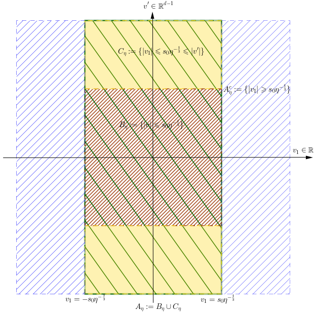
Figure 3.1: Decomposition of $\mathbb{R}^{d}$ into $A_{\eta}$ and $A_{\eta}^{c}$.

The part $A_{\eta}^{c}$ is represented by the blue zone, while the part $A_{\eta}$, in green stripes, is broken down into two other parts: the brown zone $B_{\eta}$ for $|v^{\prime}|$ small, and the yellow zone $C_{\eta}$ for $|v^{\prime}|$ large.

The parts $\tilde{A}_{\eta}$, $\tilde{C}_{\eta}$ and $D_{\eta}$ are an extensions “in the direction of $v_{1}$” of the parts $A_{\eta}$, $C_{\eta}$ and $A_{\eta}^{c}$ respectively, and are not shown in the figure above.

Step 1: Estimation of $\|M_{\lambda,\eta}\|_{L^{2}(A_{\eta}^{c})}$. We summarize this step in the following inequality:

$$\|M_{\lambda,\eta}\|^{2}_{L^{2}(A_{\eta}^{c})}\leqslant\frac{1}{s_{0}^{2}}\big{\|}\eta^{\frac{1}{3}}v_{1}M_{\lambda,\eta}\big{\|}^{2}_{L^{2}(A_{\eta}^{c})}\lesssim\frac{1}{s_{0}^{3}}\bigg{(}\|N_{\lambda,\eta}\|^{2}_{L^{2}(A_{\eta})}+c_{1}^{\eta}\bigg{)},$$ (3.2)

where $c_{1}^{\eta}=c_{1}(\lambda,\eta,s_{0})=s_{0}^{-2\delta}\eta^{\frac{2\delta}{3}}(|b(\lambda,\eta)|+1)\||v_{1}|^{\delta}M\|^{2}_{L^{2}(\mathbb{R}^{d})}$ where $\delta$ can be chosen as follows $\delta:=\frac{1}{2}(\gamma-\frac{d}{2})$ to ensure that $|v|^{\delta}M$ belongs to $L^{2}$.

$\bullet$ Estimation of $\|\eta^{\frac{1}{3}}v_{1}M_{\lambda,\eta}\|_{L^{2}(A_{\eta}^{c})}$. In order to localize the velocities on the part $A_{\eta}^{c}$ and to be able to use the equation of $M_{\lambda,\eta}$ and make integrations by part, we introduce the function $\chi_{\eta}$ defined by: $\chi_{\eta}(v_{1}):=\chi\big{(}\frac{v_{1}}{s_{0}\eta^{-1/3}}\big{)}$, where $\chi\in C^{\infty}(\mathbb{R})$ is such that $0\leqslant\chi\leqslant 1$, $\chi\equiv 0$ on $B(0,\frac{1}{2})$ and $\chi\equiv 1$ outside of $B(0,1)$. Then, one has: $\|\eta^{\frac{1}{3}}v_{1}M_{\lambda,\eta}\|_{L^{2}(A_{\eta}^{c})}\leqslant\|\eta^{\frac{1}{3}}v_{1}\chi_{\eta}M_{\lambda,\eta}\|_{L^{2}(D_{\eta})}$. Now, multiplying the equation of $M_{\lambda,\eta}$ by $v_{1}{\overline{M}}_{\lambda,\eta}\chi_{\eta}^{2}$, integrating it over $D_{\eta}$ and taking the imaginary part, we get:

$$\big{\|}\eta^{\frac{1}{3}}v_{1}\chi_{\eta}M_{\lambda,\eta}\big{\|}^{2}_{L^{2}(D_{\eta})} =-\eta^{-\frac{1}{3}}\mbox{Im}\bigg{(}\int_{D_{\eta}}Q(M_{\lambda,\eta})v_{1}{\overline{M}}_{\lambda,\eta}\chi_{\eta}^{2}\mathrm{d}v\bigg{)}+\mbox{Im}\bigg{(}\lambda\int_{D_{\eta}}\eta^{\frac{1}{3}}v_{1}|M_{\lambda,\eta}\chi_{\eta}|^{2}\mathrm{d}v\bigg{)}$$

$$\quad-\eta^{-\frac{1}{3}}\mbox{Im}\bigg{(}b(\lambda,\eta)\int_{D_{\eta}}\Phi v_{1}{\overline{M}}_{\lambda,\eta}\chi_{\eta}^{2}\mathrm{d}v\bigg{)}$$

$$=:-E^{\eta}_{1}+E^{\eta}_{2}+E^{\eta}_{3}.$$

Let’s start with $E^{\eta}_{2}$ and $E^{\eta}_{3}$ which are simpler.
$\bullet$ Estimation of $E^{\eta}_{2}$: For this term, we just use the fact that on $D_{\eta}$: $\frac{s_{0}}{2}\leqslant\eta^{\frac{1}{3}}|v_{1}|$. Thus,

$$|E^{\eta}_{2}|:=\bigg{|}\mbox{Im}\bigg{(}\lambda\int_{D_{\eta}}\eta^{\frac{1}{3}}v_{1}|M_{\lambda,\eta}\chi_{\eta}|^{2}\mathrm{d}v\bigg{)}\bigg{|}\leqslant\frac{2|\lambda|}{s_{0}}\big{\|}\eta^{\frac{1}{3}}v_{1}\chi_{\eta}M_{\lambda,\eta}\big{\|}^{2}_{L^{2}(D_{\eta})}.$$ (3.3)

$\bullet$ Estimation of $E^{\eta}_{3}$: First of all, since $\Phi(v):=\big{(}\int_{\mathbb{R}^{d}}\langle v\rangle^{-2-2\gamma}\mathrm{d}v\big{)}^{-1}\frac{M(v)}{\langle v\rangle^{2}}$ then:

$$\Phi(v)\chi_{\{|v_{i}|\geqslant s_{0}\eta^{-\frac{1}{3}}\}}(v)\leqslant Cs_{0}^{-2}\eta^{\frac{2}{3}}M(v).$$ (3.4)

In particular,

$$\Phi(v)\chi_{\eta}(v_{1})\leqslant Cs_{0}^{-2}\eta^{\frac{2}{3}}M(v).$$ (3.5)

Similarly, we have:

$$\|M\|_{L^{2}(\{|v_{i}|\geqslant s_{0}\eta^{-\frac{1}{3}}\})}\leqslant s_{0}^{-\delta}\eta^{\frac{\delta}{3}}\big{\|}|v|^{\delta}M\big{\|}_{L^{2}(\mathbb{R}^{d})}.$$ (3.6)

Then, using (3.5), we get

$$|E^{\eta}_{3}|:=\bigg{|}\eta^{-\frac{1}{3}}\mbox{Im}\bigg{(}b(\lambda,\eta)\int_{D_{\eta}}\Phi v_{1}{\overline{M}}_{\lambda,\eta}\chi_{\eta}^{2}\mathrm{d}v\bigg{)}\bigg{|}\leqslant 4\frac{|b(\lambda,\eta)|}{s_{0}^{2}}\|\chi_{\eta}M\|_{L^{2}(D_{\eta})}\big{\|}\eta^{\frac{1}{3}}v_{1}\chi_{\eta}M_{\lambda,\eta}\big{\|}_{L^{2}(D_{\eta})}.$$

Finally, by inequality (3.6)

$$|E^{\eta}_{3}|\leqslant 2\frac{|b(\lambda,\eta)|}{s_{0}^{2}}\bigg{(}\big{\|}\eta^{\frac{1}{3}}v_{1}\chi_{\eta}M_{\lambda,\eta}\big{\|}^{2}_{L^{2}(D_{\eta})}+4s_{0}^{-2\delta}\eta^{\frac{2\delta}{3}}\big{\|}|v|^{\delta}M\big{\|}_{L^{2}(\mathbb{R}^{d})}^{2}\bigg{)}.$$ (3.7)

$\bullet$ Estimation of $E^{\eta}_{1}$: By an integration by parts, we write

$$E^{\eta}_{1}:=\eta^{-\frac{1}{3}}\mbox{Im}\int_{D_{\eta}}Q(M_{\lambda,\eta})v_{1}{\overline{M}}_{\lambda,\eta}\chi_{\eta}^{2}\mathrm{d}v=\eta^{-\frac{1}{3}}\mbox{Im}\int_{D_{\eta}}\big{[}\chi_{\eta}{\overline{M}}_{\lambda,\eta}+2v_{1}\chi_{\eta}^{\prime}{\overline{M}}_{\lambda,\eta}\big{]}\partial_{v_{1}}\bigg{(}\frac{M_{\lambda,\eta}}{M}\bigg{)}M\chi_{\eta}\mathrm{d}v.$$

Thus, by Cauchy-Schwarz

$$|E^{\eta}_{1}|\leqslant\eta^{-\frac{1}{3}}\bigg{\|}\partial_{v_{1}}\bigg{(}\frac{M_{\lambda,\eta}}{M}\bigg{)}M\chi_{\eta}\bigg{\|}_{L^{2}(D_{\eta})}\bigg{(}\|\chi_{\eta}M_{\lambda,\eta}\|_{L^{2}(D_{\eta})}+2\|v_{1}\chi_{\eta}^{\prime}M_{\lambda,\eta}\|_{L^{2}(D_{\eta})}\bigg{)}.$$

Since $\chi_{\eta}^{\prime}\equiv 0$ except on: $D_{\eta}\setminus A_{\eta}^{c}=\{\frac{s_{0}}{2}\eta^{-\frac{1}{3}}\leqslant|v_{1}|\leqslant s_{0}\eta^{-\frac{1}{3}}\}\subset A_{\eta}:=\{|v_{1}|\leqslant s_{0}\eta^{-\frac{1}{3}}\}$. Then,

$$\|v_{1}\chi_{\eta}^{\prime}M_{\lambda,\eta}\|_{L^{2}(D_{\eta})}=\|v_{1}\chi_{\eta}^{\prime}M_{\lambda,\eta}\|_{L^{2}(D_{\eta}\setminus A_{\eta}^{c})}\leqslant C\|M_{\lambda,\eta}\|_{L^{2}(D_{\eta}\setminus A_{\eta}^{c})},$$

where $C=\underset{\frac{1}{2}\leqslant|t|\leqslant 1}{\mathop{\rm sup}}|t\chi^{\prime}(t)|$. Also, we have: $\|\chi_{\eta}M_{\lambda,\eta}\|_{L^{2}(D_{\eta})}\leqslant\frac{1}{s_{0}}\|\eta^{\frac{1}{3}}v_{1}\chi_{\eta}M_{\lambda,\eta}\|_{L^{2}(D_{\eta})}$. Thus,

$$|E^{\eta}_{1}|\leqslant\eta^{-\frac{1}{3}}\bigg{\|}\partial_{v_{1}}\bigg{(}\frac{M_{\lambda,\eta}}{M}\bigg{)}M\chi_{\eta}\bigg{\|}_{L^{2}(D_{\eta})}\bigg{(}\frac{1}{s_{0}}\|\eta^{\frac{1}{3}}v_{1}\chi_{\eta}M_{\lambda,\eta}\|_{L^{2}(D_{\eta})}+C\|M_{\lambda,\eta}\|_{L^{2}(D_{\eta}\setminus A_{\eta}^{c})}\bigg{)}.$$

Finally, by Young’s inequality:

$$|E^{\eta}_{1}|\lesssim s_{0}\eta^{-\frac{2}{3}}\bigg{\|}\partial_{v_{1}}\bigg{(}\frac{M_{\lambda,\eta}}{M}\bigg{)}M\chi_{\eta}\bigg{\|}^{2}_{L^{2}(D_{\eta})}+\frac{1}{s_{0}^{3}}\|\eta^{\frac{1}{3}}v_{1}\chi_{\eta}M_{\lambda,\eta}\|^{2}_{L^{2}(D_{\eta})}+\frac{1}{s_{0}}\|M_{\lambda,\eta}\|^{2}_{L^{2}(D_{\eta}\setminus A_{\eta}^{c})}.$$ (3.8)

It remains to estimate $\big{\|}\partial_{v_{1}}\big{(}\frac{M_{\lambda,\eta}}{M}\big{)}M\chi_{\eta}\big{\|}_{L^{2}(D_{\eta})}$. For this, one has

$$\bigg{\|}\partial_{v_{1}}\bigg{(}\frac{M_{\lambda,\eta}}{M}\bigg{)}M\chi_{\eta}\bigg{\|}^{2}_{L^{2}(D_{\eta})} \leqslant\bigg{\|}\nabla_{v}\bigg{(}\frac{M_{\lambda,\eta}}{M}\bigg{)}M\chi_{\eta}\bigg{\|}^{2}_{L^{2}(D_{\eta})}$$

$$=\mbox{Re}\int_{D_{\eta}}\bigg{[}Q(M_{\lambda,\eta}){\overline{M}}_{\lambda,\eta}\chi_{\eta}^{2}+2\zeta_{\eta}^{\prime}\zeta_{\eta}\frac{{\overline{M}}_{\lambda,\eta}}{M}\partial_{v_{1}}\bigg{(}\frac{M_{\lambda,\eta}}{M}\bigg{)}M^{2}\bigg{]}\mathrm{d}v$$

$$=:F^{\eta}_{1}+F^{\eta}_{2}.$$ (3.9)

By integrating the equation of $M_{\lambda,\eta}$, multiplied by ${\overline{M}}_{\lambda,\eta}\chi_{\eta}^{2}$, over $D_{\eta}$, and using (3.4), we obtain

$$|F^{\eta}_{1}|\lesssim\frac{\eta^{\frac{2}{3}}}{s_{0}^{2}}\bigg{[}\bigg{(}|\lambda|+\frac{|b(\lambda,\eta)|}{s_{0}^{2}}\bigg{)}\big{\|}\eta^{\frac{1}{3}}v_{1}\chi_{\eta}M_{\lambda,\eta}\big{\|}^{2}_{L^{2}(D_{\eta})}+|b(\lambda,\eta)|\|M\|^{2}_{L^{2}(D_{\eta})}\bigg{]}.$$ (3.10)

For $F^{\eta}_{2}$, by inequality $(2Cab\leqslant 2C^{2}a^{2}+\frac{b^{2}}{2})$:

$$|F^{\eta}_{2}| \leqslant 2\|\chi_{\eta}^{\prime}M_{\lambda,\eta}\|_{L^{2}(D_{\eta})}\bigg{\|}\partial_{v_{1}}\bigg{(}\frac{M_{\lambda,\eta}}{M}\bigg{)}M\chi_{\eta}\bigg{\|}_{L^{2}(D_{\eta})}$$

$$\leqslant 2C\frac{\eta^{\frac{1}{3}}}{s_{0}}\|M_{\lambda,\eta}\|_{L^{2}(D_{\eta}\setminus A_{\eta}^{c})}\bigg{\|}\partial_{v_{1}}\bigg{(}\frac{M_{\lambda,\eta}}{M}\bigg{)}M\chi_{\eta}\bigg{\|}_{L^{2}(D_{\eta})}$$

$$\leqslant C^{\prime}\frac{\eta^{\frac{2}{3}}}{s_{0}^{2}}\|M_{\lambda,\eta}\|^{2}_{L^{2}(D_{\eta}\setminus A_{\eta}^{c})}+\frac{1}{2}\bigg{\|}\partial_{v_{1}}\bigg{(}\frac{M_{\lambda,\eta}}{M}\bigg{)}M\chi_{\eta}\bigg{\|}^{2}_{L^{2}(D_{\eta})},$$ (3.11)

where $C=\underset{\frac{1}{2}\leqslant|t|\leqslant 1}{\mathop{\rm sup}}|t\chi^{\prime}(t)|$ and $C^{\prime}=2C^{2}$. Then, we obtain by returning to (3.1)

$$\bigg{\|}\partial_{v_{1}}\bigg{(}\frac{M_{\lambda,\eta}}{M}\bigg{)}M\chi_{\eta}\bigg{\|}^{2}_{L^{2}(D_{\eta})}\leqslant|F^{\eta}_{1}|+C^{\prime}\frac{\eta^{\frac{2}{3}}}{s_{0}^{2}}\|M_{\lambda,\eta}\|^{2}_{L^{2}(D_{\eta}\setminus A_{\eta}^{c})}+\frac{1}{2}\bigg{\|}\partial_{v_{1}}\bigg{(}\frac{M_{\lambda,\eta}}{M}\bigg{)}M\chi_{\eta}\bigg{\|}^{2}_{L^{2}(D_{\eta})}.$$

Therefore,

$$\bigg{\|}\partial_{v_{1}}\bigg{(}\frac{M_{\lambda,\eta}}{M}\bigg{)}M\chi_{\eta}\bigg{\|}^{2}_{L^{2}(D_{\eta})}\lesssim|F^{\eta}_{1}|+\frac{\eta^{\frac{2}{3}}}{s_{0}^{2}}\|M_{\lambda,\eta}\|^{2}_{L^{2}(D_{\eta}\setminus A_{\eta}^{c})}.$$

Hence, from (3.10), (3.6) and the last inequality

$$\bigg{\|}\partial_{v_{1}}\bigg{(}\frac{M_{\lambda,\eta}}{M}\bigg{)}M\chi_{\eta}\bigg{\|}^{2}_{L^{2}(D_{\eta})}\lesssim\frac{\eta^{\frac{2}{3}}}{s_{0}^{2}} \bigg{[}\bigg{(}|\lambda|+\frac{|b(\lambda,\eta)|}{s_{0}^{2}}\bigg{)}\big{\|}\eta^{\frac{1}{3}}v_{1}\chi_{\eta}M_{\lambda,\eta}\big{\|}^{2}_{L^{2}(D_{\eta})}+\|M_{\lambda,\eta}\|^{2}_{L^{2}(D_{\eta}\setminus A_{\eta}^{c})}$$

$$+s_{0}^{-2\delta}\eta^{\frac{2\delta}{3}}|b(\lambda,\eta)|\big{\|}|v_{1}|^{\delta}M\big{\|}^{2}_{L^{2}(\mathbb{R}^{d})}\bigg{]}.$$

Which implies, by inequality (3.8), that

$$|E^{\eta}_{1}|\lesssim\frac{1}{s_{0}} \bigg{[}\bigg{(}|\lambda|+\frac{1+|b(\lambda,\eta)|}{s_{0}^{2}}\bigg{)}\big{\|}\eta^{\frac{1}{3}}v_{1}\chi_{\eta}M_{\lambda,\eta}\big{\|}^{2}_{L^{2}(D_{\eta})}+\|M_{\lambda,\eta}\|^{2}_{L^{2}(D_{\eta}\setminus A_{\eta}^{c})}$$

$$+s_{0}^{-2\delta}\eta^{\frac{2\delta}{3}}|b(\lambda,\eta)|\big{\|}|v_{1}|^{\delta}M\big{\|}^{2}_{L^{2}(\mathbb{R}^{d})}\bigg{]}.$$ (3.12)

Thus, by summing the inequalities obtained from $E^{\eta}_{1}$, $E^{\eta}_{2}$ and $E^{\eta}_{3}$, namely (3.12), (3.3) and (3.7) respectively, we obtain

$$\big{\|}\eta^{\frac{1}{3}}v_{1}\chi_{\eta}M_{\lambda,\eta}\big{\|}^{2}_{L^{2}(D_{\eta})}\lesssim\frac{1}{s_{0}} \bigg{[}\bigg{(}|\lambda|+\frac{1+|b(\lambda,\eta)|}{s_{0}^{2}}\bigg{)}\big{\|}\eta^{\frac{1}{3}}v_{1}\chi_{\eta}M_{\lambda,\eta}\big{\|}^{2}_{L^{2}(D_{\eta})}+\|M_{\lambda,\eta}\|^{2}_{L^{2}(D_{\eta}\setminus A_{\eta}^{c})}$$

$$+s_{0}^{-2\delta}\eta^{\frac{2\delta}{3}}|b(\lambda,\eta)|\big{\|}|v_{1}|^{\delta}M\big{\|}^{2}_{L^{2}(\mathbb{R}^{d})}\bigg{]}.$$

Hence the following estimate

$$\big{\|}\eta^{\frac{1}{3}}v_{1}\chi_{\eta}M_{\lambda,\eta}\big{\|}^{2}_{L^{2}(D_{\eta})}\lesssim\frac{1}{s_{0}}\bigg{(}\|M_{\lambda,\eta}\|^{2}_{L^{2}(D_{\eta}\setminus A_{\eta}^{c})}+s_{0}^{-2\delta}\eta^{\frac{2\delta}{3}}|b(\lambda,\eta)|\big{\|}|v_{1}|^{\delta}M\big{\|}^{2}_{L^{2}(\mathbb{R}^{d})}\bigg{)}$$ (3.13)

holds true for $s_{0}>0$ large enough and for all $|\lambda|\leqslant\lambda_{0}$ and $\eta\in[0,\eta_{0}]$, with $\lambda_{0}$ and $\eta_{0}$ small enough. Finally, (3.2) comes from the previous inequality (3.13), and since $D_{\eta}\setminus A_{\eta}^{c}\subset A_{\eta}$ and $D_{\eta}\setminus A_{\eta}^{c}\subset D_{\eta}$ implies that,

$$\|M_{\lambda,\eta}\|^{2}_{L^{2}(D_{\eta}\setminus A_{\eta}^{c})}\leqslant\|N_{\lambda,\eta}\|^{2}_{L^{2}(A_{\eta})}+\|M\|^{2}_{L^{2}(D_{\eta})}\leqslant\|N_{\lambda,\eta}\|^{2}_{L^{2}(A_{\eta})}+4s_{0}^{-2\delta}\eta^{\frac{2\delta}{3}}\big{\|}|v_{1}|^{\delta}M\big{\|}^{2}_{L^{2}(\mathbb{R}^{d})}.$$

Step 2: Estimation of $\|N_{\lambda,\eta}\|_{L^{2}(C_{\eta})}$. In this step, we will establish the following inequality:

$$\|N_{\lambda,\eta}\|^{2}_{L^{2}(C_{\eta})}\lesssim\|N_{\lambda,\eta}\|^{2}_{L^{2}(A_{\eta}^{c})}+c_{2}^{\eta},$$ (3.14)

where $c_{2}^{\eta}:=s_{0}^{-\delta}\eta^{\frac{\delta}{3}}\big{(}s_{0}^{2}|\lambda|+s_{0}^{3}+|b(\lambda,\eta)|\big{)}\||v|^{\delta}M\|^{2}_{L^{2}(\mathbb{R}^{d})}$, and where we recall that $\delta:=\frac{1}{2}(\gamma-\frac{d}{2})$, $C_{\eta}:=\{|v_{1}|\leqslant s_{0}\eta^{-\frac{1}{3}}\leqslant|v^{\prime}|\}$ and $A_{\eta}^{c}:=\{|v_{1}|\geqslant s_{0}\eta^{-\frac{1}{3}}\}$. We start with the following Lemma:

Lemma 3.2 (Poincaré-type inequality)

Let $R>0$ be fixed and let $C_{R}$ be the set defined by: $C_{R}:=\{v\in\mathbb{R}^{d};\ |v_{1}|\leqslant R\leqslant|v^{\prime}|\}$. Then, there exists a constant $C>0$ such that, for any function $\psi$ in the space $\mathcal{H}:=\big{\{}\int_{C_{R}}\big{|}\partial_{v_{1}}\big{(}\frac{\psi}{M}\big{)}\big{|}^{2}M^{2}\mathrm{d}v<\infty;\ \psi(-R,\cdot)=\psi(R,\cdot)=0\big{\}}$, the inequality

$$\|\psi\|^{2}_{L^{2}(C_{R})}\leqslant CR^{2}\big{\|}\partial_{v_{1}}\big{(}\frac{\psi}{M}\big{)}M\big{\|}^{2}_{L^{2}(C_{R})}$$ (3.15)

holds true.

Proof of Lemma 3.2. We have for $\psi\in\mathcal{H}$: $\ \displaystyle\frac{\psi}{M}=\int_{-R}^{v_{1}}\partial_{v_{1}}\big{(}\frac{\psi}{M}\big{)}\mathrm{d}w$.
Then, by taking the square and applying the Cauchy-Schwarz inequality, we get:

$$|\psi|^{2}\leqslant M^{2}(v_{1},v^{\prime})\bigg{(}\int_{-R}^{v_{1}}\partial_{v_{1}}\bigg{(}\frac{\psi}{M}\bigg{)}\mathrm{d}w_{1}\bigg{)}^{2}\leqslant\int_{-R}^{R}\frac{M^{2}(v_{1},v^{\prime})}{M^{2}(w_{1},v^{\prime})}\mathrm{d}w_{1}\int_{-R}^{R}\bigg{|}\partial_{v_{1}}\bigg{(}\frac{\psi}{M}\bigg{)}M\bigg{|}^{2}\mathrm{d}w_{1}.$$

Now, we have for $v_{1},w_{1}\in[-R,R]$ and $|v^{\prime}|\geqslant R$, $\frac{M^{2}(v_{1},v^{\prime})}{M^{2}(w_{1},v^{\prime})}\lesssim 1$. Therefore,

$$|\psi|^{2}\lesssim R\int_{-R}^{R}\bigg{|}\partial_{v_{1}}\bigg{(}\frac{\psi}{M}\bigg{)}M\bigg{|}^{2}\mathrm{d}w_{1}.$$

Thus, we obtain the inequality (3.15) by integrating the last one over $C_{R}$.

$\square$
Now back to the estimate of $\|N_{\lambda,\eta}\|_{L^{2}(C_{\eta})}$. Let $\zeta\in C^{\infty}(\mathbb{R})$ such that $0\leqslant\zeta\leqslant 1$, $\zeta\equiv 1$ on $B(0,1)$ and $\zeta\equiv 0$ outside of $B(0,2)$. We define $\zeta_{\eta}$ by: $\zeta_{\eta}(v_{1}):=\zeta\big{(}\frac{v_{1}}{s_{0}\eta^{-1/3}}\big{)}$. Then, for $\eta>0$ and $s_{0}>0$ fixed, by applying Lemma 3.2 for $R=s_{0}\eta^{-\frac{1}{3}}$, we obtain:

$$\|N_{\lambda,\eta}\|^{2}_{L^{2}(C_{\eta})}\leqslant\|\zeta_{\eta}N_{\lambda,\eta}\|^{2}_{L^{2}(\tilde{C}_{\eta})}\lesssim\ s_{0}^{2}\eta^{-\frac{2}{3}}\bigg{\|}\partial_{v_{1}}\bigg{(}\frac{\zeta_{\eta}N_{\lambda,\eta}}{M}\bigg{)}M\bigg{\|}^{2}_{L^{2}(\tilde{C}_{\eta})},$$ (3.16)

recalling that $\tilde{C}_{\eta}:=\{|v_{1}|\leqslant 2s_{0}\eta^{-\frac{1}{3}}\leqslant 2|v^{\prime}|\}$. Furthermore,

$$\bigg{\|}\partial_{v_{1}}\bigg{(}\frac{\zeta_{\eta}N_{\lambda,\eta}}{M}\bigg{)}M\bigg{\|}^{2}_{L^{2}(\tilde{C}_{\eta})}\leqslant\bigg{\|}\nabla_{v}\bigg{(}\frac{\zeta_{\eta}N_{\lambda,\eta}}{M}\bigg{)}M\bigg{\|}^{2}_{L^{2}(\tilde{C}_{\eta})}=\mbox{Re}\int_{\tilde{C}_{\eta}}Q(\zeta_{\eta}N_{\lambda,\eta})\zeta_{\eta}{\overline{N}}_{\lambda,\eta}\mathrm{d}v.$$

However,

$$\mbox{Re}\int_{\tilde{C}_{\eta}}Q(\zeta_{\eta}N_{\lambda,\eta})\zeta_{\eta}{\overline{N}}_{\lambda,\eta}\mathrm{d}v =\mbox{Re}\int_{\tilde{C}_{\eta}}\big{[}Q(N_{\lambda,\eta}){\overline{N}}_{\lambda,\eta}\zeta_{\eta}^{2}-\zeta_{\eta}\zeta_{\eta}^{\prime\prime}|N_{\lambda,\eta}|^{2}-2\zeta_{\eta}\zeta_{\eta}^{\prime}{\overline{N}}_{\lambda,\eta}\partial_{v_{1}}N_{\lambda,\eta}\big{]}\mathrm{d}v$$

$$=\mbox{Re}\int_{\tilde{C}_{\eta}}Q(N_{\lambda,\eta}){\overline{N}}_{\lambda,\eta}\zeta_{\eta}^{2}\mathrm{d}v+\int_{\tilde{C}_{\eta}}|\zeta_{\eta}^{\prime}N_{\lambda,\eta}|^{2}\mathrm{d}v,$$ (3.17)

where we used the fact that $Q(\zeta_{\eta}N_{\lambda,\eta})=Q(N_{\lambda,\eta})\zeta_{\eta}-\zeta_{\eta}^{\prime\prime}N_{\lambda,\eta}-2\zeta_{\eta}^{\prime}\partial_{v_{1}}N_{\lambda,\eta}$ in the first line, since $Q:=-\frac{1}{M}\nabla_{v}\big{(}M^{2}\nabla\big{(}\frac{\cdot}{M}\big{)}\big{)}=-\Delta_{v}+W(v)$, and did an integration by parts for the term $\int_{\tilde{C}_{\eta}}\zeta_{\eta}\zeta_{\eta}^{\prime\prime}|N_{\lambda,\eta}|^{2}\mathrm{d}v$, and used the identity: $\mbox{Re}\big{(}{\overline{f}}\partial_{v_{1}}f\big{)}=\frac{1}{2}\partial_{v_{1}}|f|^{2}$ in the second line.
To handle $\int_{\tilde{C}_{\eta}}|\zeta_{\eta}^{\prime}N_{\lambda,\eta}|^{2}\mathrm{d}v$, we have:

$$\int_{\tilde{C}_{\eta}}|\zeta_{\eta}^{\prime}N_{\lambda,\eta}|^{2}\mathrm{d}v=\int_{\tilde{C}_{\eta}\setminus B_{\eta}^{c}}|\zeta_{\eta}^{\prime}N_{\lambda,\eta}|^{2}\mathrm{d}v\leqslant\|\zeta^{\prime}\|^{2}_{L^{\infty}(\tilde{C}_{\eta}\setminus B_{\eta}^{c})}\|N_{\lambda,\eta}\|^{2}_{L^{2}({\tilde{C}_{\eta}\setminus B_{\eta}^{c}})},$$

since $\zeta_{\eta}^{\prime}\equiv 0$ except on: $\tilde{C}_{\eta}\setminus B_{\eta}^{c}=\{s_{0}\eta^{-\frac{1}{3}}\leqslant|v_{1}|\leqslant 2s_{0}\eta^{-\frac{1}{3}}\leqslant 2|v^{\prime}|\}\subset A_{\eta}^{c}$, and that on $\tilde{C}_{\eta}\setminus B_{\eta}^{c}$ we have: $|\zeta_{\eta}^{\prime}(v_{1})|\lesssim\frac{\eta^{\frac{1}{3}}}{s_{0}}$. Then,

$$\int_{\tilde{C}_{\eta}}|\zeta_{\eta}^{\prime}N_{\lambda,\eta}|^{2}\mathrm{d}v\lesssim\frac{\eta^{\frac{2}{3}}}{s_{0}^{2}}\|N_{\lambda,\eta}\|^{2}_{L^{2}(A_{\eta}^{c})}.$$ (3.18)

To handle $\mbox{Re}\int_{\tilde{C}_{\eta}}Q(N_{\lambda,\eta}){\overline{N}}_{\lambda,\eta}\zeta_{\eta}^{2}\mathrm{d}v$, we will proceed as in $E^{\eta}_{1}$. Indeed, recall that $N_{\lambda,\eta}$ satisfies the equation:

$$Q(N_{\lambda,\eta})=(\lambda\eta^{\frac{2}{3}}-\mathrm{i}\eta v_{1})N_{\lambda,\eta}+(\lambda\eta^{\frac{2}{3}}-\mathrm{i}\eta v_{1})M-b(\lambda,\eta)\Phi.$$

Then, multiplying this equation by ${\overline{N}}_{\lambda,\eta}\zeta_{\eta}^{2}$ and integrating it over $\tilde{C}_{\eta}$, we get

$$\bigg{|}\mbox{Re}\int_{\tilde{C}_{\eta}}Q(N_{\lambda,\eta}){\overline{N}}_{\lambda,\eta}\zeta_{\eta}^{2}\mathrm{d}v\bigg{|} \lesssim|\lambda|\eta^{\frac{2}{3}}\big{(}\|\zeta_{\eta}N_{\lambda,\eta}\|^{2}_{L^{2}(\tilde{C}_{\eta})}+\|M\|^{2}_{L^{2}({\tilde{C}_{\eta}})}\big{)}+\int_{\tilde{C}_{\eta}}\big{|}\eta v_{1}M{\overline{N}}_{\lambda,\eta}\zeta_{\eta}^{2}\big{|}\mathrm{d}v$$

$$+|b(\lambda,\eta)|\int_{\tilde{C}_{\eta}}\big{|}\Phi{\overline{N}}_{\lambda,\eta}\zeta_{\eta}^{2}\big{|}\mathrm{d}v.$$ (3.19)

Note that: $\displaystyle\mbox{Re}\int_{\tilde{C}_{\eta}}\mathrm{i}\eta v_{1}|N_{\lambda,\eta}\zeta_{\eta}|^{2}\mathrm{d}v=0$. Since inequality (3.4) remains true on $\tilde{C}_{\eta}$: $|v^{\prime}|\geqslant s_{0}\eta^{-\frac{1}{3}}$, we have

$$\int_{\tilde{C}_{\eta}}\big{|}\Phi{\overline{N}}_{\lambda,\eta}\zeta_{\eta}^{2}\big{|}\mathrm{d}v \lesssim s_{0}^{-2}\eta^{\frac{2}{3}}\|M\|_{L^{2}({\tilde{C}_{\eta}})}\|N_{\lambda,\eta}\zeta_{\eta}\|_{L^{2}({\tilde{C}_{\eta}})}$$ (3.20)

$$\lesssim s_{0}^{-2-\delta}\eta^{\frac{2+\delta}{3}}\big{\|}|v^{\prime}|^{\delta}M\big{\|}_{L^{2}(\mathbb{R}^{d})}\|N_{\lambda,\eta}\zeta_{\eta}\|_{L^{2}({\tilde{C}_{\eta}})}$$

$$\lesssim s_{0}^{-2-\delta}\eta^{\frac{2+\delta}{3}}\bigg{(}\|\zeta_{\eta}N_{\lambda,\eta}\|^{2}_{L^{2}(\tilde{C}_{\eta})}+\big{\|}|v|^{\delta}M\big{\|}^{2}_{L^{2}(\mathbb{R}^{d})}\bigg{)}.$$ (3.21)

Now, the right hand term of the first line in (3.19) is treated as follows:

$$\int_{\tilde{C}_{\eta}}\big{|}\eta v_{1}M{\overline{N}}_{\lambda,\eta}\zeta_{\eta}^{2}\big{|}\mathrm{d}v \leqslant 2s_{0}^{1-\delta}\eta^{\frac{2+\delta}{3}}\|\zeta_{\eta}N_{\lambda,\eta}\|_{L^{2}(\tilde{C}_{\eta})}\big{\|}|v|^{\delta}\zeta_{\eta}M\big{\|}_{L^{2}({\tilde{C}_{\eta}})}$$

$$\leqslant s_{0}^{1-\delta}\eta^{\frac{2+\delta}{3}}\bigg{(}\|\zeta_{\eta}N_{\lambda,\eta}\|^{2}_{L^{2}(\tilde{C}_{\eta})}+\big{\|}|v|^{\delta}M\big{\|}^{2}_{L^{2}(\mathbb{R}^{d})}\bigg{)}.$$ (3.22)

Hence, from (3.16), (3.18) and the estimates obtained for the terms of (3.19) we obtain

$$\|\zeta_{\eta}N_{\lambda,\eta}\|^{2}_{L^{2}(\tilde{C}_{\eta})} \lesssim\big{(}s_{0}^{2}|\lambda|+s_{0}^{3-\delta}\eta^{\frac{\delta}{3}}+s_{0}^{-\delta}\eta^{\frac{\delta}{3}}|b(\lambda,\eta)|\big{)}\|\zeta_{\eta}N_{\lambda,\eta}\|^{2}_{L^{2}(\tilde{C}_{\eta})}+\|N_{\lambda,\eta}\|^{2}_{L^{2}(A_{\eta}^{c})}$$

$$+\eta^{\frac{\delta}{3}}\big{(}s_{0}^{2-\delta}|\lambda|+s_{0}^{3-\delta}+s_{0}^{-\delta}|b(\lambda,\eta)|\big{)}\big{\|}|v|^{\delta}M\big{\|}^{2}_{L^{2}(\mathbb{R}^{d})}.$$

So, for $s_{0}$ fixed and $|\lambda|$ and $\eta$ small enough, $\big{(}s_{0}^{2}|\lambda|+s_{0}^{3-\delta}\eta^{\frac{\delta}{3}}+s_{0}^{-\delta}\eta^{\frac{\delta}{3}}|b(\lambda,\eta)|\big{)}\leqslant\frac{1}{2}$ and the term $\|\zeta_{\eta}N_{\lambda,\eta}\|^{2}_{L^{2}(\tilde{C}_{\eta})}$ in the right side of the previous inequality is absorbed. Thus,

$$\|\zeta_{\eta}N_{\lambda,\eta}\|^{2}_{L^{2}(\tilde{C}_{\eta})}\lesssim\|N_{\lambda,\eta}\|^{2}_{L^{2}(A_{\eta}^{c})}+\eta^{\frac{\delta}{3}}\big{(}s_{0}^{2-\delta}|\lambda|+s_{0}^{3-\delta}+s_{0}^{-\delta}|b(\lambda,\eta)|\big{)}\big{\|}|v|^{\delta}M\big{\|}^{2}_{L^{2}(\mathbb{R}^{d})}.$$

Hence the inequality (3.14) holds.

Step 3: Estimation of $\|N_{\lambda,\eta}\|_{L^{2}(B_{\eta})}$. Recall that $B_{\eta}:=\{|v|\leqslant s_{0}\eta^{-\frac{1}{3}}\}$.We claim that:

$$\|N_{\lambda,\eta}\|^{2}_{L^{2}(B_{\eta})} \lesssim\nu_{1}\|N_{\lambda,\eta}\|^{2}_{L^{2}(A_{\eta})}+s_{0}^{2}|\lambda|\|N_{\lambda,\eta}\|^{2}_{L^{2}(A_{\eta}^{c})}+s_{0}^{2-\delta}\eta^{\frac{\delta}{3}}\big{\|}\eta^{\frac{1}{3}}v_{1}M_{\lambda,\eta}\big{\|}^{2}_{L^{2}(A_{\eta}^{c})}$$

$$+(s_{0}^{2}|\lambda|+|c_{\eta}-1|)\|M\|^{2}_{2}+s_{0}^{3-\delta}\eta^{\frac{\delta}{3}}\big{\|}|v_{1}|^{\delta}M\big{\|}^{2}_{2}$$ (3.23)

where $\nu_{1}:=\nu_{1}(\lambda,\eta,s_{0})=s_{0}^{2}|\lambda|+s_{0}^{3-\delta}\eta^{\frac{\delta}{3}}$ and $\displaystyle c_{\eta}:=\bigg{(}\int_{\mathbb{R}^{d}}\frac{M^{2}}{\langle v\rangle^{2}}\mathrm{d}v\bigg{)}^{-1}\int_{\mathbb{R}^{d}}\frac{MM_{\lambda,\eta}}{\langle v\rangle^{2}}\mathrm{d}v$.

Let us denote $\displaystyle\tilde{N}_{\lambda,\eta}:=M_{\lambda,\eta}-c_{\eta}M$ the orthogonal projection of $M_{\lambda,\eta}$ to $M$ for the weighted scalar product $\int\frac{\cdot}{\langle v\rangle^{2}}$. On the one hand, we have:

$$\|N_{\lambda,\eta}\|^{2}_{L^{2}(B_{\eta})}\lesssim\|\tilde{N}_{\lambda,\eta}\|^{2}_{L^{2}(B_{\eta})}+|c_{\eta}-1|\|M\|^{2}_{L^{2}(B_{\eta})}$$

and

$$\|\tilde{N}_{\lambda,\eta}\|^{2}_{L^{2}(B_{\eta})}\lesssim s_{0}^{2}\eta^{-\frac{2}{3}}\bigg{\|}\frac{\tilde{N}_{\lambda,\eta}}{\langle v\rangle}\bigg{\|}^{2}_{L^{2}(\mathbb{R}^{d})},$$

since $\langle v\rangle\lesssim s_{0}\eta^{-\frac{1}{3}}$ on $B_{\eta}$. On the other hand, applying the inequality (2.3) to $\tilde{N}_{\lambda,\eta}$ which satisfies condition (2.4), we obtain:

$$\int_{\mathbb{R}^{d}}\frac{|\tilde{N}_{\lambda,\eta}|^{2}}{\langle v\rangle^{2}}\mathrm{d}v\leqslant C_{\gamma,d}\int_{\mathbb{R}^{d}}\bigg{|}\nabla_{v}\bigg{(}\frac{N_{\lambda,\eta}}{M}\bigg{)}\bigg{|}^{2}M^{2}\mathrm{d}v.$$

Therefore,

$$\|N_{\lambda,\eta}\|^{2}_{L^{2}(B_{\eta})}\lesssim s_{0}^{2}\eta^{-\frac{2}{3}}\bigg{\|}\nabla_{v}\bigg{(}\frac{N_{\lambda,\eta}}{M}\bigg{)}M\bigg{\|}^{2}_{L^{2}(\mathbb{R}^{d})}+|c_{\eta}-1|\|M\|^{2}_{L^{2}(\mathbb{R}^{d})}.$$ (3.24)

We have moreover,

$$\bigg{\|}\nabla_{v}\bigg{(}\frac{N_{\lambda,\eta}}{M}\bigg{)}M\bigg{\|}^{2}_{L^{2}(\mathbb{R}^{d})}=\int_{\mathbb{R}^{d}}Q(N_{\lambda,\eta}){\overline{N}}_{\lambda,\eta}\mathrm{d}v.$$

Then, by integrating the equation of $N_{\lambda,\eta}$ multiplied by ${\overline{N}}_{\lambda,\eta}$, we obtain

$$\int_{\mathbb{R}^{d}}Q(N_{\lambda,\eta}){\overline{N}}_{\lambda,\eta}\mathrm{d}v+|\langle N_{\lambda,\eta},\Phi\rangle|^{2}=\mbox{Re}\int_{\mathbb{R}^{d}}\bigg{(}\lambda\eta^{\frac{2}{3}}\big{(}|N_{\lambda,\eta}|^{2}+M{\overline{N}}_{\lambda,\eta}\big{)}-\mathrm{i}\eta v_{1}M{\overline{N}}_{\lambda,\eta}\bigg{)}\mathrm{d}v.$$

From where,

$$\bigg{\|}\nabla_{v}\bigg{(}\frac{N_{\lambda,\eta}}{M}\bigg{)}M\bigg{\|}^{2}_{L^{2}(\mathbb{R}^{d})}\lesssim|\lambda|\eta^{\frac{2}{3}}\big{(}\|N_{\lambda,\eta}\|^{2}_{2}+\|M\|^{2}_{2}\big{)}+\eta\int_{\mathbb{R}^{d}}|v_{1}M\mbox{Im}N_{\lambda,\eta}|\mathrm{d}v.$$ (3.25)

For the last term, using the fact that $\ \mbox{Im}N_{\lambda,\eta}=\mbox{Im}M_{\lambda,\eta}$, we write

$$\eta^{\frac{1}{3}}\int_{\mathbb{R}^{d}}|v_{1}M\mbox{Im}N_{\lambda,\eta}|\mathrm{d}v=\int_{A_{\eta}}\eta^{\frac{1}{3}}|v_{1}|^{1-\delta}|v_{1}|^{\delta}M|\mbox{Im}N_{\lambda,\eta}|\mathrm{d}v+\int_{A_{\eta}^{c}}\eta^{\frac{1}{3}}|v_{1}\mbox{Im}M_{\lambda,\eta}|M\mathrm{d}v,$$ (3.26)

and since on $A_{\eta}:=\{|v_{1}|\leqslant s_{0}\eta^{-\frac{1}{3}}\}$ we have: $|v_{1}|^{1-\delta}\leqslant s_{0}^{1-\delta}\eta^{\frac{\delta-1}{3}}$, and on $A_{\eta}^{c}:=\{|v_{1}|\geqslant s_{0}\eta^{-\frac{1}{3}}\}$, $M(v)\leqslant s_{0}^{-\delta}\eta^{\frac{\delta}{3}}|v_{1}|^{\delta}M(v)$ then, we obtain

$$\eta^{\frac{1}{3}}\int_{\mathbb{R}^{d}}|v_{1}M\mbox{Im}N_{\lambda,\eta}|\mathrm{d}v \leqslant\frac{\eta^{\frac{\delta}{3}}}{s_{0}^{\delta}}\big{\|}|v_{1}|^{\delta}M\big{\|}_{2}\bigg{(}s_{0}\|N_{\lambda,\eta}\|_{L^{2}(A_{\eta})}+\big{\|}\eta^{\frac{1}{3}}v_{1}M_{\lambda,\eta}\big{\|}_{L^{2}(A_{\eta}^{c})}\bigg{)}$$

$$\leqslant\frac{1}{2}\frac{\eta^{\frac{\delta}{3}}}{s_{0}^{\delta}}\bigg{(}s_{0}\|N_{\lambda,\eta}\|^{2}_{L^{2}(A_{\eta})}+\big{\|}\eta^{\frac{1}{3}}v_{1}M_{\lambda,\eta}\big{\|}^{2}_{L^{2}(A_{\eta}^{c})}+2s_{0}\big{\|}|v_{1}|^{\delta}M\big{\|}^{2}_{2}\bigg{)}.$$ (3.27)

Thus, returning to (3.25) we get:

$$\bigg{\|}\nabla_{v}\bigg{(}\frac{N_{\lambda,\eta}}{M}\bigg{)}M\bigg{\|}^{2}_{L^{2}(\mathbb{R}^{d})} \lesssim\eta^{\frac{2}{3}}(|\lambda|+s_{0}^{1-\delta}\eta^{\frac{\delta}{3}})\|N_{\lambda,\eta}\|^{2}_{L^{2}(A_{\eta})}+\eta^{\frac{2}{3}}|\lambda|\|N_{\lambda,\eta}\|^{2}_{L^{2}(A_{\eta}^{c})}$$

$$+s_{0}^{-\delta}\eta^{\frac{2+\delta}{3}}\big{\|}\eta^{\frac{1}{3}}v_{1}M_{\lambda,\eta}\big{\|}^{2}_{L^{2}(A_{\eta}^{c})}+\eta^{\frac{2}{3}}|\lambda|\|M\|^{2}_{2}+s_{0}^{1-\delta}\eta^{\frac{2+\delta}{3}}\big{\|}|v_{1}|^{\delta}M\big{\|}^{2}_{L^{2}(\mathbb{R}^{d})}.$$

Hence the inequality (3.1) holds by multiplying the previous one by $s_{0}^{2}\eta^{-\frac{2}{3}}$ and adding the term $|c_{\eta}-1|\|M\|^{2}_{L^{2}(\mathbb{R}^{d})}$.

Step 4: Conclusion. In this step, we will combine all the estimates obtained in the previous steps in order to conclude. First, by summing the inequalities (3.14) and (3.1) obtained in steps 2 and 3 respectively, and since $A_{\eta}=B_{\eta}\cup C_{\eta}$, we obtain:

$$\|N_{\lambda,\eta}\|^{2}_{L^{2}(A_{\eta})} \lesssim\nu_{1}\|N_{\lambda,\eta}\|^{2}_{L^{2}(A_{\eta})}+(s_{0}^{2}|\lambda|+1)\|N_{\lambda,\eta}\|^{2}_{L^{2}(A_{\eta}^{c})}+\frac{\eta^{\frac{\delta}{3}}}{s_{0}^{\delta}}\big{\|}\eta^{\frac{1}{3}}v_{1}M_{\lambda,\eta}\big{\|}^{2}_{L^{2}(A_{\eta}^{c})}$$

$$+(s_{0}^{2}|\lambda|+|c_{\eta}-1|)\|M\|_{L^{2}(\mathbb{R}^{d})}^{2}+c_{2}^{\eta},$$ (3.28)

where $\nu_{1}:=s_{0}^{2}|\lambda|+s_{0}^{3-\delta}\eta^{\frac{\delta}{3}}$ and $c_{2}^{\eta}:=s_{0}^{-\delta}\eta^{\frac{\delta}{3}}\big{(}s_{0}^{3}+s_{0}^{2}|\lambda|+|b(\lambda,\eta)|\big{)}\big{\|}|v|^{\delta}M\big{\|}^{2}_{L^{2}(\mathbb{R}^{d})}$. Now, since

$$\|N_{\lambda,\eta}\|^{2}_{L^{2}(A_{\eta}^{c})}\lesssim\|M_{\lambda,\eta}\|^{2}_{L^{2}(A_{\eta}^{c})}+s_{0}^{-2\delta}\eta^{\frac{2\delta}{3}}\big{\|}|v_{1}|^{\delta}M\big{\|}^{2}_{L^{2}(A_{\eta}^{c})},$$

then, using inequality (3.2) for the two terms $\|M_{\lambda,\eta}\|^{2}_{L^{2}(A_{\eta}^{c})}$ (in the previous inequality) and $\big{\|}\eta^{\frac{1}{3}}v_{1}M_{\lambda,\eta}\big{\|}^{2}_{L^{2}(A_{\eta}^{c})}$ (in (3.1)), returning to inequality (3.1) we obtain:

$$\|N_{\lambda,\eta}\|^{2}_{L^{2}(A_{\eta})} \lesssim\big{(}\nu_{1}+\frac{1}{s_{0}^{3}}\big{)}\|N_{\lambda,\eta}\|^{2}_{L^{2}(A_{\eta})}+(s_{0}^{2}|\lambda|+|c_{\eta}-1|)\|M\|_{L^{2}(\mathbb{R}^{d})}^{2}+c_{2}^{\eta}.$$

Therefore, we first set $s_{0}$ large enough so that $\frac{1}{s_{0}^{3}}\leqslant\frac{1}{4}$, then for $|\lambda|$ and $\eta$ small enough so that $\nu_{1}:=s_{0}^{2}|\lambda|+s_{0}^{3-\delta}\eta^{\frac{\delta}{3}}\leqslant\frac{1}{4}$, we get:

$$\|N_{\lambda,\eta}\|^{2}_{L^{2}(A_{\eta})}\lesssim(s_{0}^{2}|\lambda|+|c_{\eta}-1|)\|M\|_{L^{2}(\mathbb{R}^{d})}^{2}+c_{2}^{\eta}\lesssim 1.$$ (3.29)

The right-hand side of the inequality above is uniformly bounded since $s_{0}^{2}|\lambda|\leqslant\frac{1}{4}$, $|c_{\eta}-1|\to 0$ and $c_{2}^{\eta}\to 0$ when $\eta$ goes $0$. Indeed, we have

$$|c_{\eta}-1| =\bigg{(}\int_{\mathbb{R}^{d}}\frac{M^{2}}{\langle v\rangle^{2}}\mathrm{d}v\bigg{)}^{-1}\bigg{|}\int_{\mathbb{R}^{d}}\frac{M(M_{\lambda,\eta}-M)}{\langle v\rangle^{2}}\mathrm{d}v\bigg{|}$$

$$\leqslant\bigg{\|}\frac{M}{\langle v\rangle}\bigg{\|}^{-1}_{2}\bigg{\|}\frac{N_{\lambda,\eta}}{\langle v\rangle}\bigg{\|}_{2}\leqslant C\|N_{\lambda,\eta}\|_{\mathcal{H}_{0}}\underset{\eta\to 0}{\longrightarrow}0.$$ (3.30)

For $c^{\eta}_{2}$, we have $c^{\eta}_{2}\lesssim\eta^{\frac{\delta}{3}}$ since $|v|^{\delta}M\in L^{2}$ for all $\gamma>\frac{d}{2}$ and since $|b(\lambda,\eta)|\lesssim 1$ thanks to the second point of Remark 2.19.

Now, we resume all the assumptions we did on $s_{0}$, $\lambda$ et $\eta$:

$$\frac{C_{1}}{s_{0}}\bigg{(}|\lambda|+\frac{1+|b(\lambda,\eta)|}{s_{0}^{2}}\bigg{)}\leqslant\frac{1}{2},\quad\frac{C_{2}}{s_{0}^{3}}\leqslant\frac{1}{4},\quad C_{3}\big{(}s_{0}^{2}|\lambda|+s_{0}^{3-\delta}\eta^{\frac{\delta}{3}}\big{)}\leqslant\frac{1}{4}$$

and

$$C_{4}\big{(}s_{0}^{2}|\lambda|+s_{0}^{3-\delta}\eta^{\frac{\delta}{3}}+s_{0}^{-\delta}\eta^{\frac{\delta}{3}}|b(\lambda,\eta)|\big{)}\leqslant\frac{1}{2}.$$

Recall that $\delta:=\frac{1}{2}(\gamma-\frac{d}{2})>0$ for all $\gamma>\frac{d}{2}$. So, if we start by setting $s_{0}$ large enough, then $\lambda$ small enough, then $\eta$ small enough, we recover all the previous inequalities.

Finally, by injecting the inequality (3.1) into (3.2), we obtain:

$$\|M_{\lambda,\eta}\|^{2}_{L^{2}(A_{\eta}^{c})}\leqslant\frac{1}{s_{0}^{2}}\big{\|}\eta^{\frac{1}{3}}v_{1}M_{\lambda,\eta}\big{\|}_{L^{2}(A_{\eta}^{c})}\lesssim\frac{1}{s_{0}^{3}}\big{(}\nu_{1}+c_{2}^{\eta}\big{)}\lesssim 1.$$ (3.31)

Hence, $N_{\lambda,\eta}$ as well as $M_{\lambda,\eta}$ are uniformly bounded in $L^{2}(\mathbb{R}^{d})$. Now, from (3.1) and (3.31) we obtain:

$$\|N_{\lambda,\eta}\|_{L^{2}(\mathbb{R}^{d})}^{2}\lesssim|\lambda|+|c_{\eta}-1|+c_{2}^{\eta}.$$

Hence the inequality (3.1) holds with $\nu_{\eta}:=|c_{\eta}-1|+c_{2}^{\eta}\underset{\eta\to 0}{\longrightarrow}0$. $\square$

3.2 Study of the constraint

In this subsection, we will show the existence of a $\mu$, a function of $\eta$, such that the constraint $\langle M_{\mu(\eta),\eta}-M,\Phi\rangle=0$ is satisfied. Let us start by giving the following result, which is a Corollary of Proposition 3.1.

Corollary 3.3

Let $M_{\lambda,\eta}$ be the solution to equation (2.19). Then, for all $\lambda\in\mathbb{C}$ such that, $|\lambda|\leqslant\lambda_{0}$ with $\lambda_{0}$ small enough, the following limit holds:

$$\underset{\eta\to 0}{\mathop{\rm lim}}\int_{\mathbb{R}^{d}}\eta^{\frac{1}{3}}v_{1}M_{\lambda,\eta}(v)M(v)\mathrm{d}v=0.$$ (3.32)

For $\lambda=0$, one has

$$\underset{\eta\to 0}{\mathop{\rm lim}}\int_{\mathbb{R}^{d}}M_{0,\eta}(v)M(v)\mathrm{d}v=\int_{\mathbb{R}^{d}}M^{2}(v)\mathrm{d}v.$$ (3.33)

Proof. For the first point, we proceed exactly as in (3.26), i.e. cutting the integral into two parts $A_{\eta}:=\{|v_{1}|\leqslant s_{0}\eta^{-\frac{1}{3}}\}$ and $A_{\eta}^{c}$, we write:

$$\bigg{|}\int_{\mathbb{R}^{d}}\eta^{\frac{1}{3}}v_{1}M_{\lambda,\eta}(v)M(v)\mathrm{d}v\bigg{|} \leqslant\eta^{\frac{1}{3}}\int_{A_{\eta}}|v_{1}|^{1-\delta}|v_{1}|^{\delta}M(v)|M_{\lambda,\eta}(v)|\mathrm{d}v$$

$$\hskip 56.9055pt+\int_{A_{\eta}^{c}}|v_{1}|^{-\delta}|v_{1}|^{\delta}M(v)|\eta^{\frac{1}{3}}v_{1}M_{\lambda,\eta}(v)|\mathrm{d}v$$

$$\leqslant s_{0}^{-\delta}\eta^{\frac{\delta}{3}}\big{\|}|v_{1}|^{\delta}M\big{\|}_{2}\bigg{(}s_{0}\|M_{\lambda,\eta}\|_{L^{2}(A_{\eta})}+\big{\|}\eta^{\frac{1}{3}}v_{1}M_{\lambda,\eta}\big{\|}_{L^{2}(A_{\eta}^{c})}\bigg{)}$$

$$\lesssim\eta^{\frac{\delta}{3}}\underset{\eta\to 0}{\longrightarrow}0,\quad\mbox{ thanks to }\eqref{N_eta sur A}\mbox{ and }\eqref{M_eta sur A^c fin}.$$

For the second point, for $\lambda=0$, we write

$$\bigg{|}\int_{\mathbb{R}^{d}}\big{[}M_{0,\eta}(v)-M(v)\big{]}M(v)\mathrm{d}v\bigg{|}\leqslant\|N_{0,\eta}\|_{L^{2}(\mathbb{R}^{d})}\|M\|_{L^{2}(\mathbb{R}^{d})},$$

and the limit (3.33) holds true thanks to the inequality (3.1) of Proposition 3.1. $\square$

Proposition 3.4 (Constraint)

Define

$$B(\lambda,\eta):=\eta^{-\frac{2}{3}}b(\lambda,\eta).$$

1. The expression of $B(\lambda,\eta)$ is given by

   $$B(\lambda,\eta)=\eta^{-\frac{2}{3}}\langle N_{\lambda,\eta},\Phi\rangle=\int_{\mathbb{R}^{d}}(\lambda-\mathrm{i}\eta^{\frac{1}{3}}v)M_{\lambda,\eta}(v)M(v)\mathrm{d}v.$$ (3.34)

2. The $\eta$ order of $B(\lambda,\eta)$ in its expansion with respect to $\lambda$ is given by

   $$\underset{\eta\rightarrow 0}{\mathop{\rm lim}}\ \frac{\partial B}{\partial\lambda}(0,\eta)=\int_{\mathbb{R}^{d}}M^{2}(v)\mathrm{d}v.$$ (3.35)

3. There exists $\tilde{\eta}_{0},\tilde{\lambda}_{0}>0$ small enough, a function $\tilde{\lambda}:\{|\eta|\leqslant\tilde{\eta}_{0}\}\longrightarrow\{|\lambda|\leqslant\tilde{\lambda}_{0}\}$ such that,
   for all $(\lambda,\eta)\in[0,\tilde{\eta}_{0}[\times\{|\lambda|<\tilde{\lambda}_{0}\}$, $\lambda=\tilde{\lambda}(\eta)$ and the constraint is satisfied:

   $$B(\lambda,\eta)=B(\tilde{\lambda}(\eta),\eta)=0.$$

Consequently, $\mu(\eta)=\eta^{\frac{2}{3}}\tilde{\lambda}(\eta)$ is the eigenvalue associated to the eigenfunction $M_{\eta}:=M_{\tilde{\lambda}(\eta),\eta}$ for the operator $\mathcal{L}_{\eta}$, and the couple $\big{(}\mu(\eta),M_{\eta}\big{)}$ is solution to the spectral problem (1.7).

Proof. 1. The first point is obtained by integrating the equation of $M_{\lambda,\eta}$ multiplied by $M$, and using the assumption $\langle M,\Phi\rangle=1$.
2. This point is exactly the limit (3.33) of Corollary 3.3.
3. The third point follows from the Implicit Function Theorem applied to the function $B$ around the point $(\lambda,\eta)=(0,0)$. $\square$

3.3 Approximation of the eigenvalue

In this subsection, we will give an approximation for the eigenvalue $\mu(\eta)$ given in Proposition 3.4. The study of this limit is based on some estimates on $M_{0,\eta}$, the solution of equation (2.1) for $\lambda=0$, as well as the solution of the rescaled equation.

Before giving the Proposition which summarizes the essential points of this subsection, we will first start by introducing the rescaled function of $M_{0,\eta}$ as well as the equation satisfied by this function. Recall that $M_{0,\eta}$ satisfies the equation:

$$\big{[}Q+\mathrm{i}\eta v_{1}\big{]}M_{0,\eta}(v)=-b(0,\eta)\Phi(v),\quad v\in\mathbb{R}^{d},$$

with $Q=-\frac{1}{M}\nabla_{v}\cdot\big{(}M^{2}\nabla_{v}\big{(}\frac{\cdot}{M}\big{)}\big{)}$ and $b(0,\eta)=\langle M_{0,\eta}-M,\Phi\rangle$. Then, the rescaled function $H_{\eta}$ defined by $H_{\eta}(s):=\eta^{-\frac{\gamma}{3}}M_{0,\eta}(\eta^{-\frac{1}{3}}s)$ is solution to the rescaled equation

$$\big{[}Q_{\eta}+\mathrm{i}s_{1}\big{]}H_{\eta}(s)=-\eta^{-\frac{\gamma+2}{3}}b(0,\eta)\Phi_{\eta}(s),\quad s\in\mathbb{R}^{d},$$ (3.36)

where

$$Q_{\eta}:=-\frac{1}{|s|_{\eta}^{-\gamma}}\nabla_{s}\cdot\bigg{(}|s|_{\eta}^{-2\gamma}\nabla_{s}\bigg{(}\frac{\cdot}{|s|_{\eta}^{-\gamma}}\bigg{)}\bigg{)}\ ,\quad|s|_{\eta}^{-\gamma}:=\eta^{-\frac{\gamma}{3}}M(\eta^{-\frac{1}{3}}s)=\big{(}\eta^{\frac{2}{3}}+|s|^{2}\big{)}^{-\frac{\gamma}{2}}$$

and

$$\Phi_{\eta}(s):=\Phi(\eta^{-\frac{1}{3}}s)=c_{\gamma,d}\ \eta^{\frac{\gamma+2}{3}}|s|_{\eta}^{-\gamma-2}.$$ (3.37)

Note that: $Q(M)=0$ implies that $Q_{\eta}(|s|_{\eta}^{-\gamma})=0$.

Proposition 3.5 (Approximation of the eigenvalue)

Let $\alpha:=\frac{2\gamma-d+2}{3}$ for all $\gamma\in(\frac{d}{2},\frac{d+4}{2})$. The eigenvalue $\mu(\eta)$ satisfies

$$\mu(\eta)=\overline{\mu}(-\eta)=\kappa|\eta|^{\alpha}\big{(}1+O(|\eta|^{\alpha})\big{)},$$ (3.38)

where $\kappa$ is a positive constant given by

$$\kappa:=-2C_{\beta}^{2}\int_{\{s_{1}>0\}}s_{1}|s|^{-\gamma}\mbox{Im}H_{0}(s)\mathrm{d}s,$$ (3.39)

and where $H_{0}$ is the unique solution to

$$\bigg{[}-\Delta_{s}+\frac{\gamma(\gamma-d+2)}{|s|^{2}}+\mathrm{i}s_{1}\bigg{]}H_{0}(s)=0,\ s\in\mathbb{R}^{d}\setminus\{0\},$$ (3.40)

satisfying

$$\int_{\{|s_{1}|\geqslant 1\}}|H_{0}(s)|^{2}\mathrm{d}s<+\infty\ \mbox{ and }\ H_{0}(s)\underset{0}{\sim}|s|^{-\gamma}.$$ (3.41)

In order to get the Proposition 3.5, we need to prove the following series of lemmas:

The first one show that the small velocities in the first direction do not participate in the limit of the diffusion coefficient.

Lemma 3.6 (Small velocities)

1. For all $\gamma\in(\frac{d+1}{2},\frac{d+4}{2})$, one has

   $$\int_{\{|v_{1}|\leqslant R\}}\bigg{|}\frac{\mbox{Im}M_{0,\eta}(v)}{\langle v\rangle}\bigg{|}^{2}\mathrm{d}v\lesssim\eta.$$ (3.42)

2. For all $\gamma\in(\frac{d}{2},\frac{d+4}{2})$

   $$\underset{\eta\to 0}{\mathop{\rm lim}}\ \eta^{1-\alpha}\int_{\{|v_{1}|\leqslant R\}}v_{1}M_{0,\eta}(v)M(v)\mathrm{d}v=0.$$ (3.43)

The second one contains some important estimates on the rescaled solution for large velocities.

Lemma 3.7 (Large velocities)

Let $s_{0}>0$ be fixed, large enough. We have the following estimates, uniform with respect to $\eta$, for the rescaled solution:

1. For all $\gamma\in(\frac{d}{2},\frac{d+1}{2})$, one has

   $$\big{\|}|s_{1}|^{\frac{1}{2}}\mbox{Im}H_{\eta}\big{\|}_{L^{2}(\{|s_{1}|\leqslant s_{0}\})}+\|s_{1}\mbox{Im}H_{\eta}\|_{L^{2}(\{|s_{1}|\geqslant s_{0}\})}\lesssim 1.$$ (3.44)

2. For all $\gamma\in(\frac{d+1}{2},\frac{d+4}{2})$, one has

   $$\bigg{\|}\frac{\mbox{Im}H_{\eta}}{|s|_{\eta}}\bigg{\|}_{L^{2}(\{|s_{1}|\leqslant s_{0}\})}+\|s_{1}\mbox{Im}H_{\eta}\|_{L^{2}(\{|s_{1}|\geqslant s_{0}\})}\lesssim 1.$$ (3.45)

Proof of Lemma 3.6. 1. By Remark 2.19, since $M_{0,\eta}$ is symmetric with respect to $v_{1}$ in the following sense: ${\overline{M}}_{{\overline{\lambda}},\eta}(-v_{1},v^{\prime})=M_{\lambda,\eta}(v_{1},v^{\prime})$ then, $\mbox{Im}M_{0,\eta}$ is odd with respect to $v_{1}$. Therefore,

$$\int_{\mathbb{R}^{d}}\frac{M\mbox{Im}M_{0,\eta}}{\langle v\rangle^{2}}\mathrm{d}v =\int_{\mathbb{R}^{d-1}}\bigg{[}\int_{-\infty}^{0}M\mbox{Im}M_{0,\eta}(v_{1},v^{\prime})\frac{\mathrm{d}v_{1}}{\langle v\rangle^{2}}+\int_{0}^{\infty}M\mbox{Im}M_{0,\eta}(v_{1},v^{\prime})\frac{\mathrm{d}v_{1}}{\langle v\rangle^{2}}\bigg{]}\mathrm{d}v^{\prime}$$

$$=\int_{\mathbb{R}^{d-1}}\int_{0}^{\infty}\bigg{[}\mbox{Im}{\overline{M}}_{0,\eta}(v_{1},v^{\prime})+\mbox{Im}M_{0,\eta}(v_{1},v^{\prime})\bigg{]}M\frac{\mathrm{d}v_{1}}{\langle v\rangle^{2}}\mathrm{d}v^{\prime}$$

$$=0.$$

Note that we used the symmetry of $M$ in the previous equalities. Thus, the function $\mbox{Im}M_{0,\eta}$ satisfies the condition (2.4). Then, by the Hardy-Poincaré inequality (2.3), there exists a positive constant $C_{\gamma,d}$ such that:

$$\int_{\{|v_{1}|\leqslant R\}}\bigg{|}\frac{\mbox{Im}M_{0,\eta}(v)}{\langle v\rangle}\bigg{|}^{2}\mathrm{d}v\leqslant\bigg{\|}\frac{\mbox{Im}M_{0,\eta}}{\langle v\rangle}\bigg{\|}^{2}_{2}\leqslant C_{\gamma,d}\bigg{\|}\nabla_{v}\bigg{(}\frac{\mbox{Im}M_{0,\eta}}{M}\bigg{)}M\bigg{\|}^{2}_{L^{2}(\mathbb{R}^{d})}.$$

Now, as in step 3 of the proof of Proposition 3.1, we have on the one hand,

$$\bigg{\|}\nabla_{v}\bigg{(}\frac{\mbox{Im}M_{0,\eta}}{M}\bigg{)}M\bigg{\|}^{2}_{2}=\int_{\mathbb{R}^{d}}Q(\mbox{Im}M_{0,\eta})\mbox{Im}M_{0,\eta}\mathrm{d}v.$$

On the other hand,

$$Q(\mbox{Im}M_{0,\eta})=\eta v_{1}\mbox{Re}M_{0,\eta}-\eta\bigg{(}\int_{\mathbb{R}^{d}}v_{1}M\mbox{Re}M_{0,\eta}\mathrm{d}v\bigg{)}\Phi.$$

Which implies that,

$$\bigg{|}\int_{\mathbb{R}^{d}}Q(\mbox{Im}M_{0,\eta})\mbox{Im}M_{0,\eta}\mathrm{d}v\bigg{|}\leqslant\eta\big{\|}|v_{1}|^{\frac{1}{2}}M_{0,\eta}\big{\|}_{2}\bigg{(}\big{\|}|v_{1}|^{\frac{1}{2}}M_{0,\eta}\big{\|}_{2}+\big{\|}|v_{1}|^{\frac{1}{2}}M\big{\|}_{2}\|M_{0,\eta}\|_{2}\|\Phi\|_{2}\bigg{)}.$$

Hence the inequality (3.42) holds thanks to $\big{(}1+|v_{1}|^{\frac{1}{2}}\big{)}M_{0,\eta}\in L^{2}(\mathbb{R}^{d})$ for $\gamma>\frac{d+1}{2}$ (Proposition 3.1).
2. First, since $v_{1}\mbox{Im}M_{0,\eta}$ and $M$ are even functions with respect to $v_{1}$, then

$$\int_{\{|v_{1}|\leqslant R\}}v_{1}M_{0,\eta}(v)M(v)\mathrm{d}v=2\int_{0}^{R}\int_{\mathbb{R}^{d-1}}v_{1}\mbox{Im}M_{0,\eta}(v)M(v)\mathrm{d}v^{\prime}\mathrm{d}v_{1}.$$ (3.46)

Case 1: $\gamma\in]\frac{d}{2},\frac{d+1}{2}]$. We have by Cauchy-Schwarz,

$$\eta^{1-\alpha}\bigg{|}\int_{0}^{R}\int_{\mathbb{R}^{d-1}}v_{1}\mbox{Im}M_{0,\eta}(v)M(v)\mathrm{d}v\bigg{|}\leqslant R\eta^{1-\alpha}\|\mbox{Im}M_{0,\eta}\|_{2}\|M\|_{2}\leqslant R\eta^{1-\alpha}\|N_{0,\eta}\|_{2}\|M\|_{2}\underset{\eta\to 0}{\longrightarrow}0,$$

since $1-\alpha=\frac{1+d-2\gamma}{3}\geqslant 0$ for all $\gamma\leqslant\frac{d+1}{2}$ and $\|\mbox{Im}M_{0,\eta}\|_{2}=\|\mbox{Im}N_{0,\eta}\|_{2}\leqslant\|N_{0,\eta}\|_{2}\underset{\eta\to 0}{\longrightarrow}0$.
Case 2: $\gamma\in]\frac{d+1}{2},\frac{d+4}{2}[$. Similary, we have by Cauchy-Schwarz,

$$\eta^{1-\alpha}\bigg{|}\int_{\{|v_{1}|\leqslant R\}}v_{1}M_{0,\eta}(v)M(v)\mathrm{d}v\bigg{|} \leqslant\eta^{1-\alpha}\big{\|}v_{1}\langle v\rangle M\big{\|}_{L^{2}(\{|v_{1}|\leqslant R\})}\bigg{\|}\frac{\mbox{Im}M_{0,\eta}}{\langle v\rangle}\bigg{\|}_{L^{2}(\{|v_{1}|\leqslant R\})}$$

$$\lesssim\eta^{2-\alpha}\underset{\eta\to 0}{\longrightarrow}0,$$

thanks to the inequality (3.42) and since $\alpha<2$ for $\gamma<\frac{d+4}{2}$ and $v_{1}\langle v\rangle M\in L^{2}(\{|v_{1}|\leqslant R\})$ for $\gamma<\frac{d+4}{2}$. $\square$

Proof of Lemma 3.7. We will establish estimates on different ranges of (rescalated) velocities, and in order to avoid long expressions in the proof, we will fix some notations of “sets” as in the proof of Proposition 3.1. Let denote $s:=(s_{1},s^{\prime})\in\mathbb{R}\times\mathbb{R}^{d-1}$. Let $s_{0}>0$. We set: $A:=\{|s_{1}|\leqslant s_{0}\}$ (resp., $\tilde{A}:=\{|s_{1}|\leqslant 2s_{0}\}$), $B:=\{|s|\leqslant s_{0}\}$, $C:=\{|s_{1}|\leqslant s_{0}\leqslant|s^{\prime}|\}$ (resp., $\tilde{C}:=\{|s_{1}|\leqslant 2s_{0}\leqslant 2|s^{\prime}|\}$) and finally $D:=\{|s_{1}|\geqslant\frac{s_{0}}{2}\}$. Also, for $\eta>0$, we denote by $\tilde{K}_{\eta}$ the function defined by $\tilde{K}_{\eta}:=H_{\eta}-c_{\eta}|s|_{\eta}^{-\gamma}$, with $c_{\eta}$ given by

$$c_{\eta}:=\bigg{(}\int_{\mathbb{R}^{d}}|s|_{\eta}^{-2\gamma-2}\mathrm{d}s\bigg{)}^{-1}\int_{\mathbb{R}^{d}}\frac{|s|_{\eta}^{-\gamma}H_{\eta}(s)}{|s|_{\eta}^{2}}\mathrm{d}s,\quad\forall\eta>0.$$

Note that

$$\int_{\mathbb{R}^{d}}\frac{|s|_{\eta}^{-\gamma}\tilde{K}_{\eta}(s)}{|s|_{\eta}^{2}}\mathrm{d}s=0.$$

Thus, $\tilde{K}_{\eta}$ satisfies the orthogonality condition (2.4) of the Hardy-Poincaré Lemma 2.5.

Remark 3.8

1. Observe that

   $$c_{\eta}:=\bigg{(}\int_{\mathbb{R}^{d}}\frac{M^{2}}{\langle v\rangle^{2}}\mathrm{d}v\bigg{)}^{-1}\int_{\mathbb{R}^{d}}\frac{M(v)M_{0,\eta}(v)}{\langle v\rangle^{2}}\mathrm{d}v.$$

   Hence, $\ \displaystyle c_{\eta}\underset{\eta\to 0}{\longrightarrow}1$ by (3.1).

2. Since ${\overline{M}}_{0,\eta}(-v_{1},v^{\prime})=M_{0,\eta}(v_{1},v^{\prime})$ for all $(v_{1},v^{\prime})\in\mathbb{R}\times\mathbb{R}^{d-1}$, then

   $$\mbox{Im}H_{\eta}(-s_{1},s^{\prime})=-\mbox{Im}H_{\eta}(s_{1},s^{\prime}),\quad\forall(s_{1},s^{\prime})\in\mathbb{R}\times\mathbb{R}^{d-1}.$$

   Therefore, $\mbox{Im}\ c_{\eta}=0$.

1. Let $\gamma\in(\frac{d}{2},\frac{d+1}{2})$. To prove the first point of this lemma, we will proceed exactly as in the proof of Proposition 3.1. We estimate $\big{\|}|s_{1}|^{\frac{1}{2}}K_{\eta}\big{\|}_{L^{2}(B)}$ using the Hardy-Poincaré inequality, $\big{\|}|s_{1}|^{\frac{1}{2}}K_{\eta}\big{\|}_{L^{2}(C)}$ using the weighted Poincaré inequality, Lemma 3.2, and estimate $\|s_{1}H_{\eta}\|_{L^{2}(A^{c})}$ using the equation of $H_{\eta}$. Thus, we obtain the inequality (3.44) by combining these estimates and since $|s_{1}|^{\frac{1}{2}}|s|_{\eta}^{-\gamma}\leqslant|s_{1}|^{\frac{1}{2}}|s|^{-\gamma}\in L^{2}(A)$ for $\gamma<\frac{d+1}{2}$.

Estimation of $\big{\|}|s_{1}|^{\frac{1}{2}}K_{\eta}\big{\|}_{L^{2}(B)}$. Recall that $B:=\{|s|\leqslant s_{0}\}$. On the one hand, we have:

$$\big{\|}|s_{1}|^{\frac{1}{2}}K_{\eta}\big{\|}^{2}_{L^{2}(B)}\lesssim\big{\|}|s_{1}|^{\frac{1}{2}}\tilde{K}_{\eta}\big{\|}^{2}_{L^{2}(B)}+|c_{\eta}-1|\big{\|}|s_{1}|^{\frac{1}{2}}|s|_{\eta}^{-\gamma}\big{\|}^{2}_{L^{2}(B)},$$

and by the Hardy-Poincaré inequality (2.3) we get

$$\big{\|}|s_{1}|^{\frac{1}{2}}\tilde{K}_{\eta}\big{\|}^{2}_{L^{2}(B)}\leqslant s_{0}^{3}\bigg{\|}\frac{\tilde{K}_{\eta}}{|s|_{\eta}}\bigg{\|}^{2}_{L^{2}(B)}\lesssim_{\gamma,d}s_{0}^{3}\bigg{\|}\nabla_{s}\bigg{(}\frac{\tilde{K}_{\eta}}{|s|_{\eta}^{-\gamma}}\bigg{)}|s|_{\eta}^{-\gamma}\bigg{\|}^{2}_{2}.$$

Therefore,

$$\big{\|}|s_{1}|^{\frac{1}{2}}K_{\eta}\big{\|}^{2}_{L^{2}(B)}\lesssim s_{0}^{3}\bigg{\|}\nabla_{s}\bigg{(}\frac{\tilde{K}_{\eta}}{|s|_{\eta}^{-\gamma}}\bigg{)}|s|_{\eta}^{-\gamma}\bigg{\|}^{2}_{2}+|c_{\eta}-1|\big{\|}|s_{1}|^{\frac{1}{2}}|s|_{\eta}^{-\gamma}\big{\|}^{2}_{L^{2}(B)}.$$ (3.47)

On the other hand, since $\nabla_{s}\big{(}\frac{\tilde{K}_{\eta}}{|s|_{\eta}^{-\gamma}}\big{)}=\nabla_{s}\big{(}\frac{K_{\eta}}{|s|_{\eta}^{-\gamma}}\big{)}$, then

$$\bigg{\|}\nabla_{s}\bigg{(}\frac{\tilde{K}_{\eta}}{|s|_{\eta}^{-\gamma}}\bigg{)}|s|_{\eta}^{-\gamma}\bigg{\|}^{2}_{2}=\mbox{Re}\int_{\mathbb{R}^{d}}Q_{\eta}(K_{\eta}){\overline{K}}_{\eta}\mathrm{d}s\leqslant\bigg{|}\mbox{Re}\int_{\mathbb{R}^{d}}\mathrm{i}s_{1}|s|_{\eta}^{-\gamma}{\overline{K}}_{\eta}\mathrm{d}s\bigg{|}=\bigg{|}\mbox{Re}\int_{\mathbb{R}^{d}}s_{1}|s|_{\eta}^{-\gamma}\mbox{Im}K_{\eta}\mathrm{d}s\bigg{|}.$$

Now, since $\mbox{Im}\ c_{\eta}=0$, by the second item of Remark 3.8, we write $|\mbox{Im}K_{\eta}|=|\mbox{Im}H_{\eta}|\leqslant|H_{\eta}|$. Thus, by splitting the integral above into two parts, on $A:=\{|s_{1}|\leqslant s_{0}\}$ and on $A^{c}$, we obtain:

$$\bigg{\|}\nabla_{s}\bigg{(}\frac{\tilde{K}_{\eta}}{|s|_{\eta}^{-\gamma}}\bigg{)}|s|_{\eta}^{-\gamma}\bigg{\|}^{2}_{2}\leqslant\big{\|}|s_{1}|^{\frac{1}{2}}|s|_{\eta}^{-\gamma}\big{\|}_{L^{2}(A)}\big{\|}|s_{1}|^{\frac{1}{2}}K_{\eta}\big{\|}_{L^{2}(A)}+\big{\|}|s|_{\eta}^{-\gamma}\big{\|}_{L^{2}(A^{c})}\big{\|}s_{1}H_{\eta}\big{\|}_{L^{2}(A^{c})}.$$

Hence, returning to (3.47), we get:

$$\big{\|}|s_{1}|^{\frac{1}{2}}K_{\eta}\big{\|}^{2}_{L^{2}(B)} \leqslant\frac{1}{4}\big{\|}|s_{1}|^{\frac{1}{2}}K_{\eta}\big{\|}^{2}_{L^{2}(A)}+Cs_{0}^{3}\big{\|}|s|^{-\gamma}\big{\|}_{L^{2}(A^{c})}\big{\|}s_{1}H_{\eta}\big{\|}_{L^{2}(A^{c})}$$

$$+C\bigg{(}s_{0}^{6}\big{\|}|s_{1}|^{\frac{1}{2}}|s|^{-\gamma}\big{\|}^{2}_{L^{2}(A)}+|c_{\eta}-1|\big{\|}|s_{1}|^{\frac{1}{2}}|s|^{-\gamma}\big{\|}^{2}_{L^{2}(B)}\bigg{)}$$ (3.48)

Estimation of $\big{\|}|s_{1}|^{\frac{1}{2}}K_{\eta}\big{\|}_{L^{2}(C)}$. Recall that $C:=\{|s_{1}|\leqslant s_{0}\leqslant|s^{\prime}|\}$. This step is identical to step 2 of the proof of Proposition 3.1. We start with estimate on $\big{\|}\zeta_{s_{0}}K_{\eta}\big{\|}^{2}_{L^{2}(\tilde{C})}$. We have by using the inequality (3.15):

$$\big{\|}\zeta_{s_{0}}K_{\eta}\big{\|}^{2}_{L^{2}(\tilde{C})}\lesssim s_{0}^{2}\bigg{\|}\partial_{s_{1}}\bigg{(}\frac{\zeta_{s_{0}}K_{\eta}}{|s|_{\eta}^{-\gamma}}\bigg{)}|s|_{\eta}^{-\gamma}\bigg{\|}^{2}_{L^{2}(\tilde{C})},$$ (3.49)

where $\zeta_{s_{0}}(s_{1}):=\zeta\big{(}\frac{s_{1}}{s_{0}}\big{)}$, with $\zeta\in C^{\infty}(\mathbb{R})$ such that: $0\leqslant\zeta\leqslant 1$, $\zeta\equiv 1$ on $B(0,1)$ and $\zeta\equiv 0$ outside of $B(0,2)$, and where $\tilde{C}:=\{|s_{1}|\leqslant 2s_{0}\leqslant 2|s^{\prime}|\}$. We have

$$\bigg{\|}\partial_{s_{1}}\bigg{(}\frac{\zeta_{s_{0}}K_{\eta}}{|s|_{\eta}^{-\gamma}}\bigg{)}|s|_{\eta}^{-\gamma}\bigg{\|}^{2}_{L^{2}(\tilde{C})}\leqslant\bigg{\|}\nabla_{s}\bigg{(}\frac{\zeta_{s_{0}}K_{\eta}}{|s|_{\eta}^{-\gamma}}\bigg{)}|s|_{\eta}^{-\gamma}\bigg{\|}^{2}_{L^{2}(\tilde{C})}=\mbox{Re}\int_{\tilde{C}}Q_{\eta}(\zeta_{s_{0}}K_{\eta})\zeta_{s_{0}}{\overline{K}}_{\eta}\mathrm{d}s.$$

On the other hand, as in (3.1):

$$\mbox{Re}\int_{\tilde{C}}Q_{\eta}(\zeta_{s_{0}}K_{\eta})\zeta_{s_{0}}{\overline{K}}_{\eta}\mathrm{d}s =\mbox{Re}\int_{\tilde{C}}Q_{\eta}(K_{\eta}){\overline{K}}_{\eta}\zeta_{s_{0}}^{2}\mathrm{d}s+\int_{\tilde{C}}|\zeta_{s_{0}}^{\prime}{\overline{K}}_{\eta}|^{2}\mathrm{d}s$$

$$\leqslant\bigg{|}\mbox{Re}\int_{\tilde{C}}-\mathrm{i}s_{1}|s|_{\eta}^{-\gamma}{\overline{K}}_{\eta}\zeta_{s_{0}}^{2}\mathrm{d}s\bigg{|}+\eta^{-\frac{2+\gamma}{3}}|b(0,\eta)|\int_{\tilde{C}}\big{|}\Phi_{\eta}{\overline{K}}_{\eta}\zeta_{s_{0}}^{2}\big{|}\mathrm{d}s$$

$$\hskip 56.9055pt+\int_{\tilde{C}}|\zeta_{s_{0}}^{\prime}K_{\eta}|^{2}\mathrm{d}s.$$

For the first term, we get

$$\bigg{|}\mbox{Re}\int_{\tilde{C}}-\mathrm{i}s_{1}|s|_{\eta}^{-\gamma}{\overline{K}}_{\eta}\zeta_{s_{0}}^{2}\mathrm{d}s\bigg{|}\leqslant\big{\|}|s_{1}|^{\frac{1}{2}}|s|_{\eta}^{-\gamma}\big{\|}_{L^{2}(\tilde{C})}\big{\|}|s_{1}|^{\frac{1}{2}}\zeta_{s_{0}}K_{\eta}\big{\|}_{L^{2}(\tilde{C})}.$$

For the second term, recall that $\Phi_{\eta}(s):=c_{\gamma,d}\ \eta^{\frac{\gamma+2}{3}}|s|_{\eta}^{-\gamma-2}$, (3.37), we get:

$$\eta^{-\frac{2+\gamma}{3}}|b(0,\eta)|\int_{\tilde{C}}\big{|}\Phi_{\eta}{\overline{K}}_{\eta}\zeta_{s_{0}}^{2}\big{|}\mathrm{d}s \lesssim s_{0}^{-\frac{5}{2}}|b(0,\eta)|\big{\|}|s_{1}|^{\frac{1}{2}}|s|_{\eta}^{-\gamma}\big{\|}_{L^{2}(\tilde{C})}\|\zeta_{s_{0}}K_{\eta}\|_{L^{2}(\tilde{C})}$$

$$\lesssim s_{0}^{-\frac{5}{2}}|b(0,\eta)|\bigg{(}\big{\|}|s_{1}|^{\frac{1}{2}}|s|^{-\gamma}\big{\|}^{2}_{L^{2}(\tilde{C})}+\|\zeta_{s_{0}}K_{\eta}\|^{2}_{L^{2}(\tilde{C})}\bigg{)}.$$

For the last term, since $\zeta_{s_{0}}^{\prime}\equiv 0$ except on $\tilde{C}\setminus B^{c}:=\{s_{0}\leqslant|s_{1}|\leqslant 2s_{0}\leqslant 2|s^{\prime}|\}$ where $|\zeta_{s_{0}}^{\prime}(s_{1})|\lesssim\frac{1}{s_{0}}$, and since $\tilde{C}\setminus B^{c}\subset A^{c}$, then

$$\int_{\tilde{C}}|\zeta_{s_{0}}^{\prime}K_{\eta}|^{2}\mathrm{d}s=\int_{\tilde{C}\setminus B^{c}}|\zeta_{s_{0}}^{\prime}K_{\eta}|^{2}\mathrm{d}s\lesssim\frac{1}{s_{0}^{2}}\|K_{\eta}\|^{2}_{L^{2}(\tilde{C}\setminus B^{c})}\lesssim\frac{1}{s_{0}^{4}}\big{\|}s_{1}H_{\eta}\big{\|}^{2}_{L^{2}(A^{c})}+\frac{1}{s_{0}^{2}}\||s|_{\eta}^{-\gamma}\|^{2}_{L^{2}(A^{c})}.$$

Therefore,

$$\|\zeta_{s_{0}}K_{\eta}\|^{2}_{L^{2}(\tilde{C})} \lesssim s_{0}^{2}\big{\|}|s_{1}|^{\frac{1}{2}}|s|^{-\gamma}\big{\|}_{L^{2}(\tilde{C})}\big{\|}|s_{1}|^{\frac{1}{2}}\zeta_{s_{0}}K_{\eta}\big{\|}_{L^{2}(\tilde{C})}+s_{0}^{-\frac{1}{2}}|b(0,\eta)|\|\zeta_{s_{0}}K_{\eta}\|^{2}_{L^{2}(\tilde{C})}$$

$$+s_{0}^{-\frac{1}{2}}|b(0,\eta)|\big{\|}|s_{1}|^{\frac{1}{2}}|s|^{-\gamma}\big{\|}^{2}_{L^{2}(\tilde{C})}+\frac{1}{s_{0}^{2}}\big{\|}s_{1}H_{\eta}\big{\|}^{2}_{L^{2}(A^{c})}+\||s|^{-\gamma}\|^{2}_{L^{2}(A^{c})}$$

Since $|b(0,\eta)|\lesssim\eta^{\frac{2}{3}}$, thanks to (3.32) and (3.34), then for $\eta$ small enough we get

$$\|\zeta_{s_{0}}K_{\eta}\|^{2}_{L^{2}(\tilde{C})} \lesssim s_{0}^{2}\big{\|}|s_{1}|^{\frac{1}{2}}|s|^{-\gamma}\big{\|}_{L^{2}(\tilde{C})}\big{\|}|s_{1}|^{\frac{1}{2}}\zeta_{s_{0}}K_{\eta}\big{\|}_{L^{2}(\tilde{C})}+\frac{1}{s_{0}^{2}}\big{\|}s_{1}H_{\eta}\big{\|}^{2}_{L^{2}(A^{c})}$$

$$+s_{0}^{-\frac{1}{2}}|b(0,\eta)|\big{\|}|s_{1}|^{\frac{1}{2}}|s|^{-\gamma}\big{\|}^{2}_{L^{2}(\tilde{C})}+\||s|^{-\gamma}\|^{2}_{L^{2}(A^{c})}.$$

Now, by (3.49), we get

$$\big{\|}|s_{1}|^{\frac{1}{2}}\zeta_{s_{0}}K_{\eta}\big{\|}^{2}_{L^{2}(\tilde{C})}\leqslant 2s_{0}\big{\|}\zeta_{s_{0}}K_{\eta}\big{\|}^{2}_{L^{2}(\tilde{C})}\lesssim s_{0}^{3}\bigg{\|}\partial_{s_{1}}\bigg{(}\frac{\zeta_{s_{0}}K_{\eta}}{|s|_{\eta}^{-\gamma}}\bigg{)}|s|_{\eta}^{-\gamma}\bigg{\|}^{2}_{L^{2}(\tilde{C})}.$$

Then,

$$\big{\|}|s_{1}|^{\frac{1}{2}}\zeta_{s_{0}}K_{\eta}\big{\|}^{2}_{L^{2}(\tilde{C})} \lesssim s_{0}^{3}\big{\|}|s_{1}|^{\frac{1}{2}}|s|^{-\gamma}\big{\|}_{L^{2}(\tilde{C})}\big{\|}|s_{1}|^{\frac{1}{2}}\zeta_{s_{0}}K_{\eta}\big{\|}_{L^{2}(\tilde{C})}+\frac{1}{s_{0}}\big{\|}s_{1}H_{\eta}\big{\|}^{2}_{L^{2}(A^{c})}$$

$$+s_{0}^{\frac{1}{2}}|b(0,\eta)|\big{\|}|s_{1}|^{\frac{1}{2}}|s|^{-\gamma}\big{\|}^{2}_{L^{2}(\tilde{C})}+s_{0}\||s|^{-\gamma}\|^{2}_{L^{2}(A^{c})}$$

Finally, since $\big{\|}|s_{1}|^{\frac{1}{2}}K_{\eta}\big{\|}^{2}_{L^{2}(C)}\leqslant\big{\|}|s_{1}|^{\frac{1}{2}}\zeta_{s_{0}}K_{\eta}\big{\|}^{2}_{L^{2}(\tilde{C})}$, we get:

$$\big{\|}|s_{1}|^{\frac{1}{2}}K_{\eta}\big{\|}^{2}_{L^{2}(C)}\lesssim\frac{1}{s_{0}}\big{\|}s_{1}H_{\eta}\big{\|}^{2}_{L^{2}(A^{c})}+s_{0}^{6}\big{\|}|s_{1}|^{\frac{1}{2}}|s|^{-\gamma}\big{\|}^{2}_{L^{2}(\tilde{C})}+s_{0}\||s|^{-\gamma}\|^{2}_{L^{2}(A^{c})}$$ (3.50)

Conclusion: Since $A=B\cup C$ then, by summing the two inequalities (3.3) and (3.50) we find:

$$\big{\|}|s_{1}|^{\frac{1}{2}}K_{\eta}\big{\|}^{2}_{L^{2}(A)} \leqslant\frac{1}{4}\big{\|}|s_{1}|^{\frac{1}{2}}K_{\eta}\big{\|}^{2}_{L^{2}(A)}+\frac{C}{s_{0}}\big{\|}s_{1}H_{\eta}\big{\|}^{2}_{L^{2}(A^{c})}+C(s_{0}^{6}+|c_{\eta}-1|)\big{\|}|s_{1}|^{\frac{1}{2}}|s|^{-\gamma}\big{\|}^{2}_{L^{2}(\tilde{A})}$$

$$+Cs_{0}^{3}\||s|^{-\gamma}\|^{2}_{L^{2}(A^{c})}$$

Hence,

$$\big{\|}|s_{1}|^{\frac{1}{2}}K_{\eta}\big{\|}^{2}_{L^{2}(A)}\lesssim\frac{1}{s_{0}}\big{\|}s_{1}H_{\eta}\big{\|}^{2}_{L^{2}(A^{c})}+(s_{0}^{6}+|c_{\eta}-1|)\big{\|}|s_{1}|^{\frac{1}{2}}|s|^{-\gamma}\big{\|}^{2}_{L^{2}(\tilde{A})}+s_{0}^{3}\big{\|}|s|^{-\gamma}\big{\|}^{2}_{L^{2}(A^{c})},$$ (3.51)

where $\tilde{A}:=\{|s_{1}|\leqslant 2s_{0}\}$. So it remains to estimate $\big{\|}s_{1}H_{\eta}\big{\|}_{L^{2}(A^{c})}$, where $A^{c}:=\{|s_{1}|\geqslant s_{0}\}$.

Estimation of $\big{\|}s_{1}H_{\eta}\big{\|}_{L^{2}(A^{c})}$. We have $\big{\|}s_{1}H_{\eta}\big{\|}_{L^{2}(A^{c})}\leqslant\big{\|}s_{1}\chi_{s_{0}}H_{\eta}\big{\|}_{L^{2}(D)}$, where $\chi_{s_{0}}(s_{1}):=\chi\big{(}\frac{s_{1}}{s_{0}}\big{)}$, with $\chi\in C^{\infty}(\mathbb{R})$ such that $0\leqslant\chi\leqslant 1$, $\chi\equiv 0$ on $B(0,\frac{1}{2})$ and $\chi\equiv 1$ outside $B(0,1)$ and where $D:=\{|s_{1}|\geqslant s_{0}\}$. Now, integrating the equation of $H_{\eta}$ against $s_{1}{\overline{H}}_{\eta}\chi_{s_{0}}^{2}$ and take the imaginary part, we obtain:

$$\int_{D}\big{|}s_{1}\chi_{s_{0}}H_{\eta}\big{|}^{2}\mathrm{d}s=-\mbox{Im}\bigg{(}\int_{D}Q_{\eta}(H_{\eta})s_{1}{\overline{H}}_{\eta}\chi_{s_{0}}^{2}\mathrm{d}s\bigg{)}-\eta^{-\frac{\gamma+2}{3}}\mbox{Im}\bigg{(}b(0,\eta)\int_{D}\Phi_{\eta}s_{1}{\overline{H}}_{\eta}\chi_{s_{0}}^{2}\mathrm{d}s\bigg{)}$$ (3.52)

Let’s start with the second term which is simpler, by (3.37) we have,

$$\eta^{-\frac{\gamma+2}{3}}\bigg{|}\mbox{Im}\bigg{(}b(0,\eta)\int_{D}\Phi_{\eta}s_{1}{\overline{H}}_{\eta}\chi_{s_{0}}^{2}\mathrm{d}s\bigg{)}\bigg{|} \lesssim\frac{1}{s_{0}^{2}}|b(0,\eta)|\||s|_{\eta}^{-\gamma}\|_{L^{2}(D)}\big{\|}s_{1}\chi_{s_{0}}H_{\eta}\big{\|}_{L^{2}(D)}$$

$$\lesssim\frac{1}{s_{0}^{2}}|b(0,\eta)|\bigg{(}\||s|^{-\gamma}\|^{2}_{L^{2}(D)}+\big{\|}s_{1}\chi_{s_{0}}H_{\eta}\big{\|}^{2}_{L^{2}(D)}\bigg{)}.$$

For the first term, we will proceed exactly as for $E^{\eta}_{1}$ (first step in the proof of the Proposition 3.1). By integration by parts, we write:

$$\bigg{|}\mbox{Im}\int_{D}Q_{\eta}(H_{\eta})s_{1}{\overline{H}}_{\eta}\chi_{s_{0}}^{2}\mathrm{d}s\bigg{|} =\bigg{|}\mbox{Im}\int_{D}\partial_{s_{1}}\bigg{(}\frac{H_{\eta}}{|s|_{\eta}^{-\gamma}}\bigg{)}|s|_{\eta}^{-\gamma}\chi_{s_{0}}\big{[}\chi_{s_{0}}{\overline{H}}_{\eta}+2s_{1}{\overline{H}}_{\eta}\chi_{s_{0}}^{\prime}\big{]}\mathrm{d}s\bigg{|}$$

$$\leqslant\bigg{\|}\partial_{s_{1}}\bigg{(}\frac{H_{\eta}}{|s|_{\eta}^{-\gamma}}\bigg{)}|s|_{\eta}^{-\gamma}\chi_{s_{0}}\bigg{\|}_{L^{2}(D)}\bigg{(}\|\chi_{s_{0}}H_{\eta}\|_{L^{2}(D)}+2\big{\|}s_{1}\chi_{s_{0}}^{\prime}H_{\eta}\big{\|}_{L^{2}(D)}\bigg{)}$$

$$\leqslant\frac{1}{2}\bigg{\|}\partial_{s_{1}}\bigg{(}\frac{H_{\eta}}{|s|_{\eta}^{-\gamma}}\bigg{)}|s|_{\eta}^{-\gamma}\chi_{s_{0}}\bigg{\|}^{2}_{L^{2}(D)}+\frac{2}{s_{0}^{2}}\|s_{1}\chi_{s_{0}}H_{\eta}\|^{2}_{L^{2}(D)}$$

$$+\frac{s_{0}}{2}\bigg{\|}\partial_{s_{1}}\bigg{(}\frac{H_{\eta}}{|s|_{\eta}^{-\gamma}}\bigg{)}|s|_{\eta}^{-\gamma}\chi_{s_{0}}\bigg{\|}^{2}_{L^{2}(D)}+\frac{1}{s_{0}}\big{\|}s_{1}\chi_{s_{0}}^{\prime}H_{\eta}\big{\|}^{2}_{L^{2}(D)}.$$

Now, since $\chi_{s_{0}}^{\prime}\equiv 0$ except on: $D\setminus A^{c}:=\{\frac{s_{0}}{2}\leqslant|s_{1}|\leqslant s_{0}\}\subset A$ where $|\chi_{s_{0}}^{\prime}(s_{1})|\lesssim\frac{1}{s_{0}}$, and since $|H_{\eta}|\leqslant|K_{\eta}|+|s|_{\eta}^{-\gamma}$ then,

$$\big{\|}s_{1}\chi_{s_{0}}^{\prime}H_{\eta}\big{\|}^{2}_{L^{2}(D)}\lesssim\|H_{\eta}\|^{2}_{L^{2}(D\setminus A^{c})} \lesssim\|K_{\eta}\|^{2}_{L^{2}(D\setminus A^{c})}+\||s|_{\eta}^{-\gamma}\|^{2}_{L^{2}(D\setminus A^{c})}$$

$$\lesssim\frac{1}{s_{0}}\bigg{(}\big{\|}|s_{1}|^{\frac{1}{2}}K_{\eta}\big{\|}^{2}_{L^{2}(A)}+\big{\|}|s_{1}|^{\frac{1}{2}}|s|_{\eta}^{-\gamma}\big{\|}^{2}_{L^{2}(A)}\bigg{)}.$$

Therefore,

$$\bigg{|}\mbox{Im}\int_{D}Q_{\eta}(H_{\eta})s_{1}{\overline{H}}_{\eta}\chi_{s_{0}}^{2}\mathrm{d}s\bigg{|} \leqslant s_{0}\bigg{\|}\partial_{s_{1}}\bigg{(}\frac{H_{\eta}}{|s|_{\eta}^{-\gamma}}\bigg{)}|s|_{\eta}^{-\gamma}\chi_{s_{0}}\bigg{\|}^{2}_{L^{2}(D)}+\frac{2}{s_{0}^{2}}\|s_{1}\chi_{s_{0}}H_{\eta}\|^{2}_{L^{2}(D)}$$

$$+\frac{C}{s_{0}^{2}}\bigg{(}\big{\|}|s_{1}|^{\frac{1}{2}}K_{\eta}\big{\|}^{2}_{L^{2}(A)}+\big{\|}|s_{1}|^{\frac{1}{2}}|s|^{-\gamma}\big{\|}^{2}_{L^{2}(A)}\bigg{)}.$$ (3.53)

Let us now deal with the term $\big{\|}\partial_{s_{1}}\big{(}\frac{H_{\eta}}{|s|_{\eta}^{-\gamma}}\big{)}|s|_{\eta}^{-\gamma}\chi_{s_{0}}\big{\|}_{L^{2}(D)}$. By an integration by parts, we can see that:

$$\bigg{\|}\nabla_{s}\bigg{(}\frac{H_{\eta}}{|s|_{\eta}^{-\gamma}}\bigg{)}|s|_{\eta}^{-\gamma}\chi_{s_{0}}\bigg{\|}^{2}_{L^{2}(D)}=\mbox{Re}\int_{D}\bigg{[}Q_{\eta}(H_{\eta}){\overline{H}}_{\eta}\chi_{s_{0}}^{2}-2\chi_{s_{0}}\chi_{s_{0}}^{\prime}\frac{{\overline{H}}_{\eta}}{|s|_{\eta}^{-\gamma}}\partial_{s_{1}}\bigg{(}\frac{H_{\eta}}{|s|_{\eta}^{-\gamma}}\bigg{)}|s|_{\eta}^{-2\gamma}\bigg{]}\mathrm{d}s.$$

Therefore,

$$\bigg{\|}\partial_{s_{1}}\bigg{(}\frac{H_{\eta}}{|s|_{\eta}^{-\gamma}}\bigg{)}|s|_{\eta}^{-\gamma}\chi_{s_{0}}\bigg{\|}^{2}_{L^{2}(D)} \leqslant\bigg{|}\mbox{Re}\int_{D}Q_{\eta}(H_{\eta}){\overline{H}}_{\eta}\chi_{s_{0}}^{2}\mathrm{d}s\bigg{|}$$

$$+2\|\chi_{s_{0}}^{\prime}H_{\eta}\|_{L^{2}(D)}\bigg{\|}\partial_{s_{1}}\bigg{(}\frac{H_{\eta}}{|s|_{\eta}^{-\gamma}}\bigg{)}|s|_{\eta}^{-\gamma}\chi_{s_{0}}\bigg{\|}_{L^{2}(D)}$$

$$\leqslant\bigg{|}\mbox{Re}\int_{D}Q_{\eta}(H_{\eta}){\overline{H}}_{\eta}\chi_{s_{0}}^{2}\mathrm{d}s\bigg{|}$$

$$+2\|\chi_{s_{0}}^{\prime}H_{\eta}\|^{2}_{L^{2}(D)}+\frac{1}{2}\bigg{\|}\partial_{s_{1}}\bigg{(}\frac{H_{\eta}}{|s|_{\eta}^{-\gamma}}\bigg{)}|s|_{\eta}^{-\gamma}\chi_{s_{0}}\bigg{\|}^{2}_{L^{2}(D)}.$$

Which implies that,

$$\bigg{\|}\partial_{s_{1}}\bigg{(}\frac{H_{\eta}}{|s|_{\eta}^{-\gamma}}\bigg{)}|s|_{\eta}^{-\gamma}\chi_{s_{0}}\bigg{\|}^{2}_{L^{2}(D)} \leqslant 2\bigg{|}\mbox{Re}\int_{D}Q_{\eta}(H_{\eta}){\overline{H}}_{\eta}\chi_{s_{0}}^{2}\mathrm{d}s\bigg{|}+4\|\chi_{s_{0}}^{\prime}H_{\eta}\|^{2}_{L^{2}(D\setminus A^{c})}$$

$$\lesssim\frac{1}{s_{0}^{2}}\bigg{(}|b(0,\eta)|\||s|_{\eta}^{-\gamma}\|_{L^{2}(D)}\|\chi_{s_{0}}H_{\eta}\|_{L^{2}(D)}+\|H_{\eta}\|^{2}_{L^{2}(D\setminus A^{c})}\bigg{)}$$

$$\lesssim\frac{1}{s_{0}^{3}}|b(0,\eta)|\bigg{(}\big{\|}s_{1}\chi_{s_{0}}H_{\eta}\big{\|}^{2}_{L^{2}(D)}+\||s|^{-\gamma}\|^{2}_{L^{2}(D)}\bigg{)}$$

$$+\frac{1}{s_{0}^{3}}\bigg{(}\big{\|}|s_{1}|^{\frac{1}{2}}K_{\eta}\big{\|}^{2}_{L^{2}(A)}+\big{\|}|s_{1}|^{\frac{1}{2}}|s|^{-\gamma}\big{\|}^{2}_{L^{2}(A)}\bigg{)}.$$

Thus, injecting this last inequality into (3.3) we obtain:

$$\bigg{|}\mbox{Im}\int_{D}Q_{\eta}(H_{\eta})s_{1}{\overline{H}}_{\eta}\chi_{s_{0}}^{2}\mathrm{d}s\bigg{|} \lesssim\frac{1}{s_{0}^{2}}\bigg{[}(1+|b(0,\eta)|)\|s_{1}\chi_{s_{0}}H_{\eta}\|^{2}_{L^{2}(D)}+\big{\|}|s_{1}|^{\frac{1}{2}}K_{\eta}\big{\|}^{2}_{L^{2}(A)}$$

$$+\big{\|}|s_{1}|^{\frac{1}{2}}|s|^{-\gamma}\big{\|}^{2}_{L^{2}(A)}+|b(0,\eta)|\||s|^{-\gamma}\|^{2}_{L^{2}(D)}\bigg{]},$$

and going back to (3.52), using the fact that $|b(0,\eta)|\lesssim 1$ by Remark 2.19, we get:

$$\|s_{1}\chi_{s_{0}}H_{\eta}\|^{2}_{L^{2}(D)} \lesssim\frac{1}{s_{0}^{2}}\bigg{[}\|s_{1}\chi_{s_{0}}H_{\eta}\|^{2}_{L^{2}(D)}+\big{\|}|s_{1}|^{\frac{1}{2}}K_{\eta}\big{\|}^{2}_{L^{2}(A)}+\big{\|}|s_{1}|^{\frac{1}{2}}|s|^{-\gamma}\big{\|}^{2}_{L^{2}(A)}+\||s|^{-\gamma}\|^{2}_{L^{2}(D)}\bigg{]}.$$

Finally, for $s_{0}$ large enough, the term $\frac{1}{s_{0}^{2}}\|s_{1}\chi_{s_{0}}H_{\eta}\|^{2}_{L^{2}(D)}$ is absorbed and we obtain thanks to the inequality $\|s_{1}H_{\eta}\|^{2}_{L^{2}(A^{c})}\leqslant\|s_{1}\chi_{s_{0}}H_{\eta}\|^{2}_{L^{2}(D)}$:

$$\|s_{1}H_{\eta}\|^{2}_{L^{2}(A^{c})}\lesssim\frac{1}{s_{0}^{2}}\bigg{(}\big{\|}|s_{1}|^{\frac{1}{2}}K_{\eta}\big{\|}^{2}_{L^{2}(A)}+\big{\|}|s_{1}|^{\frac{1}{2}}|s|^{-\gamma}\big{\|}^{2}_{L^{2}(A)}+\||s|^{-\gamma}\|^{2}_{L^{2}(D)}\bigg{)}.$$ (3.54)

Now, by injecting the inequality (3.54) into (3.51), we get:

$$\big{\|}|s_{1}|^{\frac{1}{2}}K_{\eta}\big{\|}^{2}_{L^{2}(A)}\leqslant C\bigg{(}\frac{1}{s_{0}^{3}}\big{\|}|s_{1}|^{\frac{1}{2}}K_{\eta}\big{\|}^{2}_{L^{2}(A)}+s_{0}^{6}\big{\|}|s_{1}|^{\frac{1}{2}}|s|_{\eta}^{-\gamma}\big{\|}^{2}_{L^{2}(\tilde{A})}+s_{0}^{3}\big{\|}|s|_{\eta}^{-\gamma}\big{\|}^{2}_{L^{2}(D)}\bigg{)}.$$

Where we used the fact that $A^{c}\subset D$ and $|c_{\eta}-1|\lesssim 1$ by Remark 3.8. Finally, for $s_{0}$ large enough, the norm $\big{\|}|s_{1}|^{\frac{1}{2}}K_{\eta}\big{\|}^{2}_{L^{2}(A)}$ which appears in the right hand side of the previous inequality is absorbed, from where:

$$\big{\|}|s_{1}|^{\frac{1}{2}}K_{\eta}\big{\|}^{2}_{L^{2}(A)}\lesssim s_{0}^{6}\big{\|}|s_{1}|^{\frac{1}{2}}|s|^{-\gamma}\big{\|}^{2}_{L^{2}(\tilde{A})}+s_{0}^{3}\big{\|}|s|^{-\gamma}\big{\|}^{2}_{L^{2}(A^{c})}\lesssim 1,$$ (3.55)

since for $\gamma\in]\frac{d}{2},\frac{d+1}{2}[$: $|s_{1}|^{\frac{1}{2}}|s|^{-\gamma}\in L^{2}(\tilde{A})$ and $|s|^{-\gamma}\in L^{2}(A^{c})$. From the inequality (3.54) we deduce that $\big{\|}|s_{1}|^{\frac{1}{2}}K_{\eta}\big{\|}^{2}_{L^{2}(A)}\lesssim 1$ implies that $\|s_{1}H_{\eta}\|^{2}_{L^{2}(A^{c})}\lesssim 1$. Thus we obtain (3.44).

2. Recall that $\tilde{K}_{\eta}:=H_{\eta}-c_{\eta}|s|_{\eta}^{-\gamma}$ satisfies the orthogonality condition (2.4) of Hardy-Poincaré inequality (2.3) and that $\mbox{Im}c_{\eta}=0$. It follows that, $\mbox{Im}\tilde{K}_{\eta}=\mbox{Im}K_{\eta}=\mbox{Im}H_{\eta}$, so by (2.3), we get on the one hand

$$\bigg{\|}\frac{\mbox{Im}H_{\eta}}{|s|_{\eta}}\bigg{\|}^{2}_{L^{2}(A)}=\bigg{\|}\frac{\mbox{Im}\tilde{K}_{\eta}}{|s|_{\eta}}\bigg{\|}^{2}_{L^{2}(A)}\leqslant\bigg{\|}\frac{\tilde{K}_{\eta}}{|s|_{\eta}}\bigg{\|}^{2}_{2}\lesssim_{\gamma,d}\bigg{\|}\nabla_{s}\bigg{(}\frac{\tilde{K}_{\eta}}{|s|_{\eta}^{-\gamma}}\bigg{)}|s|_{\eta}^{-\gamma}\bigg{\|}^{2}_{2}=\bigg{\|}\nabla_{s}\bigg{(}\frac{K_{\eta}}{|s|_{\eta}^{-\gamma}}\bigg{)}|s|_{\eta}^{-\gamma}\bigg{\|}^{2}_{2}.$$

On the other hand,

$$\bigg{\|}\nabla_{s}\bigg{(}\frac{K_{\eta}}{|s|_{\eta}^{-\gamma}}\bigg{)}|s|_{\eta}^{-\gamma}\bigg{\|}^{2}_{2}=\int_{\mathbb{R}^{d}}Q_{\eta}(K_{\eta}){\overline{K}}_{\eta}\mathrm{d}s=\mbox{Re}\bigg{(}-\mathrm{i}\int_{\mathbb{R}^{d}}s_{1}|s|_{\eta}^{-\gamma}{\overline{K}}_{\eta}\mathrm{d}s\bigg{)}-\eta^{-\frac{\gamma+2}{3}}b(0,\eta)\int_{\mathbb{R}^{d}}\Phi_{\eta}{\overline{K}}_{\eta}\mathrm{d}s.$$

We have: $b(0,\eta)\int_{\mathbb{R}^{d}}\Phi_{\eta}{\overline{K}}_{\eta}\mathrm{d}s\geqslant 0$. Indeed, by performing the change of variable $s=\eta^{\frac{1}{3}}v$, we obtain:

$$\int_{\mathbb{R}^{d}}\Phi_{\eta}{\overline{K}}_{\eta}\mathrm{d}s=\eta^{\frac{\gamma+d}{3}}\int_{\mathbb{R}^{d}}\Phi{\overline{N}}_{0,\eta}\mathrm{d}v=\eta^{\frac{\gamma+d}{3}}\overline{b(0,\eta)}.$$

Now, since $\displaystyle\mbox{Re}\bigg{(}-i\int_{\mathbb{R}^{d}}s_{1}|s|_{\eta}^{-\gamma}{\overline{K}}_{\eta}\mathrm{d}s\bigg{)}=\int_{\mathbb{R}^{d}}s_{1}|s|_{\eta}^{-\gamma}\mbox{Im}K_{\eta}\mathrm{d}s$, then we write:

$$\bigg{\|}\nabla_{s}\bigg{(}\frac{K_{\eta}}{|s|_{\eta}^{-\gamma}}\bigg{)}|s|_{\eta}^{-\gamma}\bigg{\|}^{2}_{2} \leqslant\int_{\mathbb{R}^{d}}|s_{1}|s|_{\eta}^{-\gamma}\mbox{Im}K_{\eta}|\mathrm{d}s$$

$$=\int_{A}|s_{1}|s|_{\eta}^{-\gamma}\mbox{Im}K_{\eta}|\mathrm{d}s+\int_{A^{c}}|s_{1}|s|_{\eta}^{-\gamma}\mbox{Im}H_{\eta}|\mathrm{d}s$$ (3.56)

$$\leqslant\big{\|}s_{1}|s|^{1-\gamma}\big{\|}_{L^{2}(A)}\bigg{\|}\frac{\mbox{Im}\tilde{K}_{\eta}}{|s|_{\eta}}\bigg{\|}_{L^{2}(A)}$$

$$\quad+s_{0}^{-\frac{1}{2}}\big{\|}|s_{1}|^{\frac{1}{2}}|s|^{-\gamma}\big{\|}_{L^{2}(A^{c})}\|s_{1}H_{\eta}\|_{L^{2}(A^{c})}.$$ (3.57)

It remains to estimate the norm $\|s_{1}H_{\eta}\|_{L^{2}(A^{c})}$. Recall that $D:=\{|s_{1}|\geqslant\frac{s_{0}}{2}\}$. We start by estimating $\|s_{1}\chi_{s_{0}}H_{\eta}\|_{L^{2}(D)}$. We have; as before; the two equalities:

$$\int_{D}\big{|}s_{1}\chi_{s_{0}}H_{\eta}\big{|}^{2}\mathrm{d}s=-\mbox{Im}\bigg{(}\int_{D}Q_{\eta}(H_{\eta})s_{1}{\overline{H}}_{\eta}\chi_{s_{0}}^{2}\mathrm{d}s\bigg{)}-\eta^{-\frac{\gamma+2}{3}}\mbox{Im}\bigg{(}b(0,\eta)\int_{D}\Phi_{\eta}s_{1}{\overline{H}}_{\eta}\chi_{s_{0}}^{2}\mathrm{d}s\bigg{)}$$

and

$$\bigg{|}\mbox{Im}\int_{D}Q_{\eta}(H_{\eta})s_{1}{\overline{H}}_{\eta}\chi_{s_{0}}^{2}\mathrm{d}s\bigg{|}=\bigg{|}\mbox{Im}\int_{D}\partial_{s_{1}}\bigg{(}\frac{H_{\eta}}{|s|_{\eta}^{-\gamma}}\bigg{)}\chi_{s_{0}}|s|_{\eta}^{-\gamma}\big{[}\chi_{s_{0}}{\overline{H}}_{\eta}+2s_{1}{\overline{H}}_{\eta}\chi_{s_{0}}^{\prime}\big{]}\mathrm{d}s\bigg{|}.$$

The term on the right in the first equality is treated in the same way as before and we have:

$$\eta^{-\frac{\gamma+2}{3}}\bigg{|}\mbox{Im}\bigg{(}b(0,\eta)\int_{D}\Phi_{\eta}s_{1}{\overline{H}}_{\eta}\chi_{s_{0}}^{2}\mathrm{d}s\bigg{)}\bigg{|} \lesssim s_{0}^{-\frac{5}{2}}|b(0,\eta)|\big{\|}|s_{1}|^{\frac{1}{2}}|s|_{\eta}^{-\gamma}\big{\|}_{L^{2}(D)}\big{\|}s_{1}\chi_{s_{0}}H_{\eta}\big{\|}_{L^{2}(D)}$$

$$\lesssim s_{0}^{-\frac{5}{2}}|b(0,\eta)|\bigg{(}\big{\|}|s_{1}|^{\frac{1}{2}}|s|_{\eta}^{-\gamma}\big{\|}^{2}_{L^{2}(D)}$$

$$\hskip 71.13188pt+\big{\|}s_{1}\chi_{s_{0}}H_{\eta}\big{\|}^{2}_{L^{2}(D)}\bigg{)}$$ (3.58)

For the left term in the first equality we write:

$$\bigg{|}\mbox{Im}\int_{D}\partial_{s_{1}}\bigg{(}\frac{H_{\eta}}{|s|_{\eta}^{-\gamma}}\bigg{)}\chi_{s_{0}}|s|_{\eta}^{-\gamma}\big{[}\chi_{s_{0}}{\overline{H}}_{\eta}+2s_{1}{\overline{H}}_{\eta}\chi_{s_{0}}^{\prime}\big{]}\mathrm{d}s\bigg{|}\leqslant I^{\eta}_{1}+I^{\eta}_{2}.$$

where

$$I^{\eta}_{1}:=\bigg{|}\mbox{Im}\int_{D}\chi_{s_{0}}{\overline{H}}_{\eta}\partial_{s_{1}}\bigg{(}\frac{H_{\eta}}{|s|_{\eta}^{-\gamma}}\bigg{)}\chi_{s_{0}}|s|_{\eta}^{-\gamma}\mathrm{d}s\bigg{|}\quad\mbox{and}\quad I^{\eta}_{2}:=\bigg{|}\mbox{Im}\int_{D}s_{1}\chi_{s_{0}}{\overline{H}}_{\eta}\partial_{s_{1}}\bigg{(}\frac{H_{\eta}}{|s|_{\eta}^{-\gamma}}\bigg{)}|s|_{\eta}^{-\gamma}\chi_{s_{0}}^{\prime}\mathrm{d}s\bigg{|}.$$

Then we write

$$I^{\eta}_{1} \leqslant\|\chi_{s_{0}}H_{\eta}\|_{L^{2}(D)}\bigg{\|}\partial_{s_{1}}\bigg{(}\frac{H_{\eta}}{|s|_{\eta}^{-\gamma}}\bigg{)}\chi_{s_{0}}|s|_{\eta}^{-\gamma}\bigg{\|}_{L^{2}(D)}$$

$$\leqslant\frac{1}{s_{0}}\|s_{1}\chi_{s_{0}}H_{\eta}\|_{L^{2}(D)}\bigg{\|}\nabla_{s}\bigg{(}\frac{H_{\eta}}{|s|_{\eta}^{-\gamma}}\bigg{)}|s|_{\eta}^{-\gamma}\bigg{\|}_{2}$$

$$\leqslant\frac{1}{2s_{0}}\bigg{(}\|s_{1}\chi_{s_{0}}H_{\eta}\|^{2}_{L^{2}(D)}+\bigg{\|}\nabla_{s}\bigg{(}\frac{H_{\eta}}{|s|_{\eta}^{-\gamma}}\bigg{)}|s|_{\eta}^{-\gamma}\bigg{\|}^{2}_{2}\bigg{)},$$ (3.59)

and

$$I^{\eta}_{2} \leqslant\|s_{1}\chi_{s_{0}}H_{\eta}\|_{L^{2}(D)}\|\chi_{s_{0}}^{\prime}\|_{L^{\infty}(D\setminus A^{c})}\bigg{\|}\partial_{s_{1}}\bigg{(}\frac{H_{\eta}}{|s|_{\eta}^{-\gamma}}\bigg{)}|s|_{\eta}^{-\gamma}\bigg{\|}_{L^{2}(D)}$$

$$\lesssim\frac{1}{s_{0}}\bigg{(}\|s_{1}\chi_{s_{0}}H_{\eta}\|^{2}_{L^{2}(D)}+\bigg{\|}\nabla_{s}\bigg{(}\frac{H_{\eta}}{|s|_{\eta}^{-\gamma}}\bigg{)}|s|_{\eta}^{-\gamma}\bigg{\|}^{2}_{2}\bigg{)}.$$ (3.60)

Hence, by the inequalities (3.3), (3.3) and (3.3) to estimate $\|s_{1}\chi_{s_{0}}H_{\eta}\|^{2}_{L^{2}(D)}$, and by inequality (3.57) to estimate $\big{\|}\nabla_{s}\big{(}\frac{H_{\eta}}{|s|_{\eta}^{-\gamma}}\big{)}|s|_{\eta}^{-\gamma}\big{\|}^{2}_{2}$, we get:

$$\|s_{1}\chi_{s_{0}}H_{\eta}\|^{2}_{L^{2}(D)} \lesssim\frac{1}{s_{0}}\big{\|}s_{1}|s|^{1-\gamma}\big{\|}_{L^{2}(A)}\bigg{\|}\frac{\mbox{Im}\tilde{K}_{\eta}}{|s|_{\eta}}\bigg{\|}_{L^{2}(A)}+s_{0}^{-\frac{3}{2}}\big{\|}|s_{1}|^{\frac{1}{2}}|s|^{-\gamma}\big{\|}_{L^{2}(A^{c})}\|s_{1}H_{\eta}\|_{L^{2}(A^{c})}$$

$$+\frac{1}{s_{0}}\|s_{1}\chi_{s_{0}}H_{\eta}\|^{2}_{L^{2}(D)}+s_{0}^{-\frac{5}{2}}|b(0,\eta)|\bigg{(}\big{\|}|s_{1}|^{\frac{1}{2}}|s|^{-\gamma}\big{\|}^{2}_{L^{2}(D)}+\big{\|}s_{1}\chi_{s_{0}}H_{\eta}\big{\|}^{2}_{L^{2}(D)}\bigg{)}$$

$$\lesssim\frac{1}{s_{0}}\big{\|}s_{1}|s|^{1-\gamma}\big{\|}_{L^{2}(A)}\bigg{\|}\frac{\mbox{Im}\tilde{K}_{\eta}}{|s|_{\eta}}\bigg{\|}_{L^{2}(A)}+\frac{1}{s_{0}}\|s_{1}\chi_{s_{0}}H_{\eta}\|^{2}_{L^{2}(D)}+\frac{1}{s_{0}^{3/2}}\big{\|}|s_{1}|^{\frac{1}{2}}|s|^{-\gamma}\big{\|}^{2}_{L^{2}(D)}.$$

Hence, for $s_{0}$ large enough and since $\|s_{1}H_{\eta}\|^{2}_{L^{2}(A^{c})}\leqslant\|s_{1}\chi_{s_{0}}H_{\eta}\|^{2}_{L^{2}(D)}$:

$$\|s_{1}H_{\eta}\|^{2}_{L^{2}(A^{c})}\lesssim\frac{1}{s_{0}}\bigg{\|}\frac{\mbox{Im}H_{\eta}}{|s|_{\eta}}\bigg{\|}^{2}_{L^{2}(A)}+\frac{1}{s_{0}}\big{\|}s_{1}|s|^{1-\gamma}\big{\|}^{2}_{L^{2}(A)}+s_{0}^{-\frac{3}{2}}\big{\|}|s_{1}|^{\frac{1}{2}}|s|^{-\gamma}\big{\|}^{2}_{L^{2}(D)}.$$ (3.61)

So, going back to (3.57) and using inequality $ab\leqslant Ca^{2}+\frac{b^{2}}{4C}$, we get:

$$\bigg{\|}\frac{\mbox{Im}H_{\eta}}{|s|_{\eta}}\bigg{\|}^{2}_{L^{2}(A)}\leqslant C\bigg{\|}\nabla_{s}\bigg{(}\frac{K_{\eta}}{|s|_{\eta}^{-\gamma}}\bigg{)}|s|_{\eta}^{-\gamma}\bigg{\|}^{2}_{2} \leqslant\frac{1}{4}\bigg{\|}\frac{\mbox{Im}H_{\eta}}{|s|_{\eta}}\bigg{\|}^{2}_{L^{2}(A)}+C^{2}\big{\|}s_{1}|s|^{1-\gamma}\big{\|}^{2}_{L^{2}(A)}$$

$$+\frac{C}{2}\big{\|}|s_{1}|^{\frac{1}{2}}|s|^{-\gamma}\big{\|}^{2}_{L^{2}(D)}+\frac{C}{2s_{0}}\|s_{1}H_{\eta}\|^{2}_{L^{2}(A^{c})}$$

Thus, by (3.61) we obtain

$$\bigg{\|}\frac{\mbox{Im}H_{\eta}}{|s|_{\eta}}\bigg{\|}^{2}_{L^{2}(A)}\leqslant\bigg{(}\frac{1}{4}+\frac{C^{\prime}}{s_{0}^{2}}\bigg{)}\bigg{\|}\frac{\mbox{Im}H_{\eta}}{|s|_{\eta}}\bigg{\|}^{2}_{L^{2}(A)}+C^{\prime}\bigg{(}\big{\|}s_{1}|s|^{1-\gamma}\big{\|}^{2}_{L^{2}(A)}+\big{\|}|s_{1}|^{\frac{1}{2}}|s|^{-\gamma}\big{\|}^{2}_{L^{2}(D)}\bigg{)}.$$

Finally, for $s_{0}$large enough

$$\bigg{\|}\frac{\mbox{Im}H_{\eta}}{|s|_{\eta}}\bigg{\|}^{2}_{L^{2}(A)}\lesssim\big{\|}s_{1}|s|^{1-\gamma}\big{\|}^{2}_{L^{2}(A)}+\big{\|}|s_{1}|^{\frac{1}{2}}|s|^{-\gamma}\big{\|}^{2}_{L^{2}(D)}\lesssim 1.$$ (3.62)

By (3.61), it follows that $\|s_{1}H_{\eta}\|^{2}_{L^{2}(A^{c})}\lesssim 1$. Note that for $\gamma\in]\frac{d+1}{2},\frac{d+4}{2}[$ we have:

$$s_{1}|s|_{\eta}|s|_{\eta}^{-\gamma}\leqslant s_{1}|s|^{1-\gamma}\in L^{2}(A)\ \mbox{ and }\ |s_{1}|^{\frac{1}{2}}|s|_{\eta}^{-\gamma}\leqslant|s_{1}|^{\frac{1}{2}}|s|^{-\gamma}\in L^{2}(A^{c}).$$

Hence the inequality (3.45) holds. $\square$

The third Lemma contains some complementary estimates on the rescaled solution.

Lemma 3.9 (Complementary estimates)

For all $\eta\in[0,\eta_{0}]$ and for all $\gamma\in(\frac{d}{2},\frac{d+4}{2})$, the following estimate holds

$$\bigg{\|}\frac{H_{\eta}-c_{\eta}|s|_{\eta}^{-\gamma}}{|s|_{\eta}}\bigg{\|}_{L^{2}(\mathbb{R}^{d})}\lesssim_{\gamma,d}\bigg{\|}\nabla_{s}\bigg{(}\frac{H_{\eta}}{|s|_{\eta}^{-\gamma}}\bigg{)}|s|_{\eta}^{-\gamma}\bigg{\|}_{L^{2}(\mathbb{R}^{d})}\lesssim 1.$$ (3.63)

The last one gives the formula of the diffusion coefficient.

Lemma 3.10

We have the following limit:

$$\underset{\eta\rightarrow 0}{\mathop{\rm lim}}\ \mathrm{i}\eta^{1-\alpha}\int_{\{|v_{1}|\geqslant R\}}vM_{0,\eta}(v)M(v)\mathrm{d}v=-2\int_{0}^{\infty}\int_{\mathbb{R}^{d-1}}s_{1}|s|^{-\gamma}\mbox{Im}H_{0}(s)\mathrm{d}s,$$ (3.64)

where $H_{0}$ is the unique solution to (3.40) satisfying the conditions (3.41).

Proof of Lemma 3.9. We have by the Hardy-Poincaré inequality and the inequality (3.56):

$$\Lambda_{\gamma,d}\bigg{\|}\frac{H_{\eta}-c_{\eta}|s|_{\eta}^{-\gamma}}{|s|_{\eta}}\bigg{\|}^{2}_{L^{2}(\mathbb{R}^{d})} \leqslant\bigg{\|}\nabla_{s}\bigg{(}\frac{H_{\eta}-|s|_{\eta}^{-\gamma}}{|s|_{\eta}^{-\gamma}}\bigg{)}|s|_{\eta}^{-\gamma}\bigg{\|}^{2}_{L^{2}(\mathbb{R}^{d})}$$

$$\leqslant\int_{\mathbb{R}^{d}}|s_{1}||s|_{\eta}^{-\gamma}|\mbox{Im}H_{\eta}|\mathrm{d}s$$

$$=\int_{\{|s_{1}|\leqslant s_{0}\}}|s_{1}||s|_{\eta}^{-\gamma}|\mbox{Im}H_{\eta}|\mathrm{d}s+\int_{\{|s_{1}|\geqslant s_{0}\}}|s_{1}||s|_{\eta}^{-\gamma}|\mbox{Im}H_{\eta}|\mathrm{d}s.$$

Case 1: $\gamma\in(\frac{d}{2},\frac{d+1}{2})$. By Cauchy-Schwarz and inequality (3.44) of Lemma 3.7 we get:

$$\int_{\{|s_{1}|\leqslant s_{0}\}}|s_{1}|s|_{\eta}^{-\gamma}|\mbox{Im}H_{\eta}|\mathrm{d}s\leqslant\big{\|}|s_{1}|^{\frac{1}{2}}|s|_{\eta}^{-\gamma}\big{\|}_{L^{2}(\{|s_{1}|\leqslant s_{0}\})}\big{\|}|s_{1}|^{\frac{1}{2}}\mbox{Im}H_{\eta}\big{\|}_{L^{2}(\{|s_{1}|\leqslant s_{0}\})}\lesssim 1$$

and

$$\int_{\{|s_{1}|\geqslant s_{0}\}}|s_{1}||s|_{\eta}^{-\gamma}|\mbox{Im}H_{\eta}|\mathrm{d}s\leqslant\big{\|}|s|_{\eta}^{-\gamma}\big{\|}_{L^{2}(\{|s_{1}|\geqslant s_{0}\})}\big{\|}s_{1}H_{\eta}\big{\|}_{L^{2}(\{|s_{1}|\geqslant s_{0}\})}\lesssim 1.$$

Case 2: $\gamma\in(\frac{d+1}{2},\frac{d+4}{2})$. Similary, by Cauchy-Schwarz and inequality (3.45) we get:

$$\int_{\{|s_{1}|\leqslant s_{0}\}}|s_{1}||s|_{\eta}^{-\gamma}|\mbox{Im}H_{\eta}|\mathrm{d}s\leqslant\big{\|}s_{1}|s|_{\eta}^{1-\gamma}\big{\|}_{L^{2}(\{|s_{1}|\leqslant s_{0}\})}\bigg{\|}\frac{\mbox{Im}H_{\eta}}{|s|_{\eta}}\bigg{\|}_{L^{2}(\{|s_{1}|\leqslant s_{0}\})}\lesssim 1$$

and

$$\int_{\{|s_{1}|\geqslant s_{0}\}}|s_{1}||s|_{\eta}^{-\gamma}|\mbox{Im}H_{\eta}|\mathrm{d}s\leqslant\big{\|}|s|_{\eta}^{-\gamma}\big{\|}_{L^{2}(\{|s_{1}|\geqslant s_{0}\})}\big{\|}s_{1}H_{\eta}\big{\|}_{L^{2}(\{|s_{1}|\geqslant s_{0}\})}\lesssim 1.$$

This completes the proof of the Lemma. $\square$

Proof of Lemma 3.10. First of all, since ${\overline{M}}_{0,\eta}(-v_{1},v^{\prime})=M_{0,\eta}(v_{1},v^{\prime})$ and $M(-v_{1},v^{\prime})=M(v_{1},v^{\prime})$ for all $v_{1}\in\mathbb{R}$ and for all $v^{\prime}\in\mathbb{R}^{d-1}$, thus

$$\mathrm{i}\int_{\{|v_{1}|\geqslant R\}}v_{1}M_{0,\eta}(v)M(v)\mathrm{d}v=-2\int_{\{v_{1}\geqslant R\}}v_{1}\mbox{Im}M_{0,\eta}(v)M(v)\mathrm{d}v.$$

Then, in order to compute the limit

$$\underset{\eta\rightarrow 0}{\mathop{\rm lim}}\ \mathrm{i}\eta^{\frac{d+1-2\gamma}{3}}\int_{\{|v_{1}|\geqslant R\}}v_{1}M_{0,\eta}(v)M(v)\mathrm{d}v=-2\underset{\eta\rightarrow 0}{\mathop{\rm lim}}\ \eta^{\frac{d+1-2\gamma}{3}}\int_{\{v_{1}\geqslant R\}}v_{1}\mbox{Im}M_{0,\eta}(v)M(v)\mathrm{d}v,$$

we proceed to a change of variable $v=\eta^{-\frac{1}{3}}s$, which means that we compute

$$\underset{\eta\rightarrow 0}{\mathop{\rm lim}}\ \int_{\{|s_{1}|\geqslant\eta^{\frac{1}{3}}R\}}s_{1}|s|_{\eta}^{-\gamma}\mbox{Im}H_{\eta}(s)\mathrm{d}s.$$

For that purpose, we use the weak-strong convergence in the Hilbert space $L^{2}(\mathbb{R}_{+}\times\mathbb{R}^{d-1})$.

The estimates of Lemma 3.7 imply that the sequence $\mathsf{H}_{\eta}$ defined by

$$\mathsf{H}_{\eta}(s):=\left\{\begin{array}[]{l}s_{1}^{\frac{1}{2}}\mbox{Im}H_{\eta}(s),\qquad\ \ \qquad\gamma\in(\frac{d}{2},\frac{d+1}{2}],0<s_{1}\leqslant s_{0},\\ \\ |s|_{\eta}^{-1}\mbox{Im}H_{\eta}(s),\ \qquad\quad\ \gamma\in(\frac{d+1}{2},\frac{d+4}{2}),0<s_{1}\leqslant s_{0},\\ \\ s_{1}\mbox{Im}H_{\eta}(s)\ \quad\mbox{ for all }\ \ \gamma\in(\frac{d}{2},\frac{d+4}{2})\mbox{ and }s_{1}\geqslant s_{0},\end{array}\right.$$

is bounded in $L^{2}(\mathbb{R}^{d})$, uniformly with respect to $\eta$, which implies that $\mathsf{H}_{\eta}$ converges weakly in $L^{2}(\mathbb{R}^{d})$, up to a subsequence. Let’s identify this limit that we denote by $\mathsf{H}_{0}\in L^{2}(\mathbb{R}^{d})$. We have on the one hand, $H_{\eta}$ converges to $H_{0}$ in $\mathcal{D}^{\prime}(\mathbb{R}^{d}\setminus\{0\})$. Indeed, recall that $H_{\eta}$ satisfies the equation

$$\bigg{[}-\Delta_{s}+\frac{\gamma(\gamma-d+2)}{|s|^{2}_{\eta}}+\mathrm{i}s_{1}\bigg{]}H_{\eta}(s)=\eta^{\frac{2}{3}}\frac{\gamma(\gamma+2)}{|s|^{4}_{\eta}}H_{\eta}(s)-\eta^{-\frac{2+\gamma}{3}}b(0,\eta)\Phi_{\eta}(s).$$

Let $\varphi\in\mathcal{D}(\mathbb{R}^{d}\setminus\{0\})$. Then, by integrating the previous equation against $\varphi$, we obtain:

$$\int_{\mathbb{R}^{d}\setminus\{0\}}\bigg{[}-\Delta_{s}+\frac{\gamma(\gamma-d+2)}{|s|^{2}_{\eta}}+\mathrm{i}s_{1}\bigg{]}\varphi(s)H_{\eta}(s)\mathrm{d}s =\eta^{\frac{2}{3}}\int_{\mathbb{R}^{d}\setminus\{0\}}\frac{\gamma(\gamma+2)}{|s|^{4}_{\eta}}\varphi(s)H_{\eta}(s)\mathrm{d}s$$

$$-\eta^{-\frac{2+\gamma}{3}}b(0,\eta)\int_{\mathbb{R}^{d}\setminus\{0\}}\Phi_{\eta}(s)\varphi(s)\mathrm{d}s.$$

Thanks to the uniform bound (3.63) and since $\Phi_{\eta}(s)\lesssim\eta^{\frac{2+\gamma}{3}}|s|^{-2-\gamma}$ and $b(0,\eta)\to 0$ then, passing to the limit when $\eta$ goes to $0$ in the last equality, we obtain that $H_{\eta}$ converges to $H_{0}$ in $\mathcal{D}^{\prime}(\mathbb{R}^{d}\setminus\{0\})$, solution to the equation

$$\bigg{[}-\Delta_{s}+\frac{\gamma(\gamma-d+2)}{|s|^{2}}+is_{1}\bigg{]}H_{0}(s)=0.$$ (3.65)

Moreover, for all $\gamma\in(\frac{d}{2},\frac{d+4}{2})$, the function $H_{\eta}$ satisfies the estimate

$$\bigg{\|}\frac{H_{\eta}-c_{\eta}|s|_{\eta}^{-\gamma}}{|s|_{\eta}}\bigg{\|}_{L^{2}(\{|s_{1}|\leqslant s_{0}\})}+\|s_{1}H_{\eta}\|_{L^{2}(\{|s_{1}|\geqslant s_{0}\})}\lesssim 1,$$

thanks to the inequality (3.63) and the first point of Lemma 3.7 for $\gamma\in(\frac{d}{2},\frac{d+1}{2}]$, and thanks to the second point of Lemma 3.7 for $\gamma\in(\frac{d+1}{2},\frac{d+4}{2})$. Therefore $H_{0}$ satisfies the estimate

$$\bigg{\|}\frac{H_{0}-|s|^{-\gamma}}{|s|}\bigg{\|}_{L^{2}(\{|s_{1}|\leqslant s_{0}\})}+\|s_{1}H_{0}\|_{L^{2}(\{|s_{1}|\geqslant s_{0}\})}\lesssim 1.$$

Now, $\|s_{1}H_{0}\|_{L^{2}(\{|s_{1}|\geqslant s_{0}\})}\lesssim 1$ implies that $H_{0}\in L^{2}(\{|s_{1}|\geqslant 1\})$ and $\big{\|}\frac{H_{0}-|s|^{-\gamma}}{|s|}\big{\|}_{L^{2}(\{|s_{1}|\leqslant s_{0})}\lesssim 1$ implies that $H_{0}(s)\underset{0}{\sim}|s|^{-\gamma}$, a different behaviour near zero would make the latter norm infinite. These two conditions imply that $H_{0}$ is the unique solution of the equation (3.65). Thanks to the uniqueness of this limit, the whole sequence $\mathsf{H}_{\eta}$ converges weakly to

$$\mathsf{H}_{0}(s):=\left\{\begin{array}[]{l}s_{1}^{\frac{1}{2}}\mbox{Im}H_{0}(s),\ \ \ \quad\qquad\gamma\in(\frac{d}{2},\frac{d+1}{2}],0<s_{1}\leqslant s_{0},\\ \\ |s|^{-1}\mbox{Im}H_{0}(s),\ \ \quad\quad\ \gamma\in(\frac{d+1}{2},\frac{d+4}{2}),0<s_{1}\leqslant s_{0},\\ \\ s_{1}\mbox{Im}H_{0}(s)\ \quad\mbox{ for all }\ \gamma\in(\frac{d}{2},\frac{d+4}{2})\mbox{ and }s_{1}\geqslant s_{0}.\end{array}\right.$$

Finally, we conclude by passing to the limit in the scalar product $\langle\mathsf{H}_{\eta},\mathsf{I}_{\eta}\rangle$, where $\mathsf{I}_{\eta}$ definded by

$$\mathsf{I}_{\eta}:=\left\{\begin{array}[]{l}s_{1}^{\frac{1}{2}}|s|_{\eta}^{-\gamma},\quad\qquad\gamma\in(\frac{d}{2},\frac{d+1}{2}],\ 0<|s_{1}|\leqslant s_{0},\\ \\ s_{1}|s|_{\eta}^{1-\gamma},\quad\quad\ \ \gamma\in(\frac{d+1}{2},\frac{d+4}{2}),\ 0<s_{1}\leqslant s_{0},\\ \\ |s|_{\eta}^{-\gamma},\qquad\qquad\gamma\in(\frac{d}{2},\frac{d+4}{2}),\ s_{1}\geqslant s_{0},\end{array}\right.$$

converges strongly in $L^{2}(\mathbb{R}_{+}\times\mathbb{R}^{d-1})$ to

$$\mathsf{I}_{0}:=\left\{\begin{array}[]{l}s_{1}^{\frac{1}{2}}|s|^{-\gamma},\quad\qquad\gamma\in(\frac{d}{2},\frac{d+1}{2}],\ 0<s_{1}\leqslant s_{0},\\ \\ s_{1}|s|^{1-\gamma},\quad\quad\ \ \gamma\in(\frac{d+1}{2},\frac{d+4}{2}),\ 0<s_{1}\leqslant s_{0},\\ \\ |s|^{-\gamma},\qquad\qquad\gamma\in(\frac{d}{2},\frac{d+4}{2}),\ s_{1}\geqslant s_{0}.\end{array}\right.$$

Hence the limit (3.64) holds true. $\square$

Proof of Proposition 3.5. By doing an expansion in $\lambda$ for $B$ and by Proposition 3.4, we get

$$B(\lambda,\eta)=\eta^{-\frac{2}{3}}b(\lambda,\eta)=\eta^{-\frac{2}{3}}b(0,\eta)+\lambda\int_{\mathbb{R}^{d}}M_{0,\eta}M\mathrm{d}v+O(\lambda^{2}).$$

Then, for $\lambda=\tilde{\lambda}(\eta)$ and since $B(\tilde{\lambda}(\eta),\eta)=0$, we obtain:

$$\tilde{\lambda}(\eta)=-\eta^{-\frac{2}{3}}b(0,\eta)\bigg{(}\int_{\mathbb{R}^{d}}M_{0,\eta}M\mathrm{d}v\bigg{)}^{-1}+o\big{(}\eta^{-\alpha}b(0,\eta)\big{)},$$

which implies that

$$\eta^{-\alpha}\mu(\eta)=\eta^{\frac{2}{3}-\alpha}\tilde{\lambda}(\eta)=-\eta^{-\alpha}b(0,\eta)\bigg{(}\int_{\mathbb{R}^{d}}M_{0,\eta}M\mathrm{d}v\bigg{)}^{-1}.$$

By (3.33) and (3.64),

$$\underset{\eta\rightarrow 0}{\mathop{\rm lim}}\int_{\mathbb{R}^{d}}M_{0,\eta}(v)M(v)\mathrm{d}v=\|M\|^{2}_{2}=C_{\beta}^{-2}$$

and

$$\underset{\eta\rightarrow 0}{\mathop{\rm lim}}\ \eta^{-\alpha}b(0,\eta)=2C_{\beta}^{2}\int_{0}^{\infty}\int_{\mathbb{R}^{d-1}}s_{1}|s|^{-\gamma}\mbox{Im}H_{0}(s)\mathrm{d}s^{\prime}\mathrm{d}s_{1}$$

respectively. Hence, $\underset{\eta\rightarrow 0}{\mathop{\rm lim}}\eta^{-\alpha}\mu(\eta)=\kappa$. For $\eta\in[-\eta_{0},0]$, the symmetry $\mu(\eta)=\overline{\mu}(-\eta)$ holds by complex conjugation on the equation. So it remains to prove the positivity of $\kappa$. By integrating the equation of $M_{\eta}:=M_{\tilde{\lambda}(\eta),\eta}$ against ${\overline{M}}_{\eta}$ we obtain:

$$\int_{\mathbb{R}^{d}}\bigg{|}\nabla_{v}\bigg{(}\frac{M_{\eta}}{M}\bigg{)}\bigg{|}^{2}M^{2}\mathrm{d}v+\mathrm{i}\eta\int_{\mathbb{R}^{d}}v_{1}|M_{\eta}|^{2}\mathrm{d}v=\mu(\eta)\int_{\mathbb{R}^{d}}|M_{\eta}|^{2}\mathrm{d}v.$$

Now, taking the real part and using the equality $\displaystyle\mu(\eta)\|M_{\eta}\|_{2}^{2}=\kappa\eta^{\alpha}\big{(}1+o(\eta^{\alpha})\big{)}$ we get:

$$\int_{\mathbb{R}^{d}}\bigg{|}\nabla_{v}\bigg{(}\frac{M_{\eta}}{M}\bigg{)}\bigg{|}^{2}M^{2}\mathrm{d}v=\kappa\eta^{\alpha}\big{(}1+o(\eta^{\alpha})\big{)}.$$ (3.66)

Therefore, multiplying this last equality by $\eta^{-\alpha}$ and performing the change of variable $v=\eta^{-\frac{1}{3}}s$ we obtain:

$$\int_{\mathbb{R}^{d}}\bigg{|}\nabla_{s}\bigg{(}\frac{H_{\eta}}{|s|_{\eta}^{-\gamma}}\bigg{)}\bigg{|}^{2}|s|_{\eta}^{-2\gamma}\mathrm{d}s=\kappa\big{(}1+o_{\eta}(1)\big{)}.$$

Thus, $\kappa\geqslant 0$. If $\kappa=0$ then,

$$\int_{\mathbb{R}^{d}}\bigg{|}\nabla_{s}\bigg{(}\frac{H_{0}}{|s|^{-\gamma}}\bigg{)}\bigg{|}^{2}|s|^{-2\gamma}\mathrm{d}s\leqslant\liminf\int_{\mathbb{R}^{d}}\bigg{|}\nabla_{s}\bigg{(}\frac{H_{\eta}}{|s|_{\eta}^{-\gamma}}\bigg{)}\bigg{|}^{2}|s|_{\eta}^{-2\gamma}\mathrm{d}s=0.$$

Therefore, $H_{0}=|s|^{-\gamma}$. Which leads to a contradiction since $H_{0}$ is solution to equation (3.40). Hence, the proof of Proposition 3.5 is complete. $\square$

Proof of Theorem 1.1. The existence of the eigen-solution $(\mu(\eta),M_{\eta})$ is given by Proposition 3.4. The limit (1.8) follows from the inequality (3.1) for $|\lambda|=|\tilde{\lambda}(\eta)|\lesssim\eta^{\frac{2\gamma-d}{3}}\underset{\eta\to 0}{\longrightarrow}0$, thanks to (3.38), with the limit (2.20) obtained by Theorem 2.18. Finally, the second point of Theorem 1.1 is given by Proposition 3.5.

4 Derivation of the fractional diffusion equation

The goal of this section is to prove Theorem 1.2. The proof was taken from Section 3 in [21] and adapted for the dimension $d$.

Let’s start by defining the two weighted $L^{p}$ spaces, $L^{p}_{F^{1-p}}(\mathbb{R}^{d})$ and $Y^{p}_{F}(\mathbb{R}^{2d})$:

$$L^{p}_{F^{1-p}}(\mathbb{R}^{d}):=\left\{f:\mathbb{R}^{d}\rightarrow\mathbb{R},\int_{\mathbb{R}^{d}}|f|^{p}\ F^{1-p}\ \mathrm{d}v<\infty\right\}\ \mbox{ and }\ Y^{p}_{F}(\mathbb{R}^{2d}):=L^{p}\big{(}\mathbb{R}^{d},L^{p}_{F^{1-p}}(\mathbb{R}^{d})\big{)}.$$

Recall that our goal is to show that the solution $f^{\varepsilon}$ of the Fokker-Planck equation (1.3) converges; weakly star in $L^{\infty}\left([0,T],L^{2}_{F^{-1}}(\mathbb{R}^{2})\right)$; towards $\rho(t,x)F(v)$ when $\varepsilon$ goes to $0$, where $\rho$ is the solution of the following fractional diffusion equation:

$$\partial_{t}\rho+\kappa(-\Delta)^{\frac{\beta+1}{6}}\rho=0,\quad\rho(0,x)=\int_{\mathbb{R}^{d}}f_{0}\mathrm{d}v.$$ (4.1)

Remark 4.1

Note that we will work with the Fourier transform of $\rho$ and we will prove that $\hat{\rho}(t,\xi)=\int e^{-\mathrm{i}x\cdot\xi}\rho(t,x)\mathrm{d}x$ satisfies

$$\partial_{t}\hat{\rho}+\kappa|\xi|^{\frac{\beta+1}{3}}\hat{\rho}=0.$$ (4.2)

4.1 A priori estimates

We start by recalling the following compactness lemma:

Lemma 4.2

$\cite[cite]{[\@@bibref{}{LebPu}{}{}]},\cite[cite]{[\@@bibref{}{NaPu}{}{}]}$ For initial datum $f_{0}\in Y^{p}_{F}(\mathbb{R}^{2d})$ where $p\geqslant 2$ and a positive time $T$.

1. The solution $f^{\varepsilon}$ of (1.3) is bounded in $L^{\infty}\big{(}[0,T];Y^{p}_{F}(\mathbb{R}^{2d})\big{)}$ uniformly with respect to $\varepsilon$ since it satisfies

   $$\|f^{\varepsilon}(T)\|^{p}_{Y^{p}_{F}(\mathbb{R}^{2d})}+\frac{p(p-1)}{\theta(\varepsilon)}\int_{0}^{T}\int_{\mathbb{R}^{2d}}\bigg{|}\nabla_{v}\bigg{(}\frac{f^{\varepsilon}}{F}\bigg{)}\bigg{|}^{2}\bigg{|}\frac{f^{\varepsilon}}{F}\bigg{|}^{p-2}\ F\ \mathrm{d}v\mathrm{d}x\mathrm{d}t\leqslant\|f_{0}\|^{p}_{Y^{p}_{F}(\mathbb{R}^{2d})}.$$ (4.3)

2. The density $\rho^{\varepsilon}(t,x)=\int_{\mathbb{R}^{d}}f^{\varepsilon}\ \mathrm{d}v$ is such that

   $$\|\rho^{\varepsilon}(t)\|^{p}_{p}\leqslant C_{\beta}^{-2(p-1)}\|f_{0}\|^{p}_{Y^{p}_{F}(\mathbb{R}^{2d})}\quad\mbox{ for all }\quad t\in[0,T].$$ (4.4)

3. Up to a subsequence, the density $\rho^{\varepsilon}$ converges weakly star in $L^{\infty}\big{(}[0,T];L^{p}(\mathbb{R}^{d})\big{)}$ to $\rho$.

4. Up to a subsequence, the sequence $f^{\varepsilon}$ converges weakly star in $L^{\infty}\big{(}[0,T];Y^{p}_{F}(\mathbb{R}^{2d})\big{)}$ to the function $f=\rho(t,x)F(v)$.

As a consequence, we have the following estimate:

Corollary 4.3

[21] Let $F=C_{\beta}^{2}M^{2}$ with $M=(1+|v|^{2})^{-\frac{\gamma}{2}}$ and $\beta=2\gamma\in(d,d+4)$. Let $f^{\varepsilon}$ solution to (1.3) with $\theta(\varepsilon)=\varepsilon^{\frac{2\gamma-d+2}{3}}$. Assume that $\|f_{0}/F\|_{\infty}\leqslant C$. Then $g^{\varepsilon}=f^{\varepsilon}F^{-\frac{1}{2}}$ satisfies the following estimate

$$\int_{0}^{T}\int_{\mathbb{R}^{d}}\left(\int_{\mathbb{R}^{d}}\big{|}g^{\varepsilon}-\rho^{\varepsilon}F^{\frac{1}{2}}\big{|}^{2}\mathrm{d}v\right)^{\frac{2\gamma-d+2}{2\gamma-d}}ds\mathrm{d}x\leqslant C\varepsilon^{\frac{2\gamma-d+2}{3}}.$$ (4.5)

Proof. Recall the Nash type inequality [8][26] [1]: for any $h$ such that $\int hF\mathrm{d}v=0$, we have

$$\int_{\mathbb{R}^{d}}h^{2}F\mathrm{d}v\leqslant C\left(\int_{\mathbb{R}^{d}}\big{|}\nabla_{v}h\big{|}^{2}F\mathrm{d}v\right)^{\frac{2\gamma-d}{2\gamma-d+2}}(\|h\|_{\infty}^{2})^{\frac{2}{2\gamma-d+2}}\ .$$ (4.6)

Define $h=g^{\varepsilon}F^{-\frac{1}{2}}-\rho^{\varepsilon}=\frac{f^{\varepsilon}}{F}-\rho^{\varepsilon}$, define $\alpha=\frac{2\gamma-d+2}{3}$. Observe that from $\|f\|_{L^{p}_{F^{1-p}}(\mathbb{R}^{2d})}=\big{\|}\frac{f}{F}\big{\|}_{L^{p}_{F}}$ and Lemma 4.2, formula (4.3), we have

$$\|h_{0}\|_{L^{\infty}}=\mathop{\rm lim}_{p\rightarrow\infty}\|h_{0}\|_{L^{p}_{F^{1-p}}(\mathbb{R}^{2d})}\geqslant\mathop{\rm lim}_{p\rightarrow\infty}\|h\|_{L^{p}_{F^{1-p}}(\mathbb{R}^{2d})}\geqslant\|h\|_{L^{\infty}}\ .$$

Thus by Lemma 4.2, formula (4.3) taking $p=2$, we get

$$\begin{array}[]{rcl}\displaystyle\int_{0}^{T}\int_{\mathbb{R}^{d}}\left(\int_{\mathbb{R}^{d}}|g^{\varepsilon}-\rho^{\varepsilon}F^{\frac{1}{2}}|^{2}\mathrm{d}v\right)^{\frac{2\gamma-d+2}{2\gamma-d}}\mathrm{d}s\mathrm{d}x&=&\displaystyle\int_{0}^{T}\int_{\mathbb{R}^{d}}\left(\int_{\mathbb{R}^{d}}h^{2}F\mathrm{d}v\right)^{\frac{2\gamma-d+2}{2\gamma-d}}\mathrm{d}s\mathrm{d}x\\ &\leqslant&\displaystyle C\int_{0}^{T}\int_{\mathbb{R}^{d}}\left(\int_{\mathbb{R}^{d}}\big{|}\nabla_{v}h\big{|}^{2}F\mathrm{d}v\right)(\|h\|_{\infty}^{2})^{\frac{2}{2\gamma-d}}\mathrm{d}s\mathrm{d}x\\ &\displaystyle\leqslant&C\displaystyle\int_{0}^{T}\int_{\mathbb{R}^{d}}\bigg{(}\int_{\mathbb{R}^{d}}\bigg{|}\nabla_{v}\bigg{(}\frac{f^{\varepsilon}}{F}\bigg{)}\bigg{|}^{2}F\mathrm{d}v\bigg{)}\mathrm{d}s\mathrm{d}x\leqslant C\varepsilon^{\alpha}.\end{array}$$

$\square$

4.2 Weak limit and proof of Theorem 1.2

By solving equation (1.6), we write

$$\hat{g}^{\varepsilon}(t,\xi,v)=e^{-t\theta(\varepsilon)\mathcal{L}_{\eta}}\hat{g}(0,\xi,v),$$

which gives going back to the rescaled space variable $x$

$$g^{\varepsilon}(t,x,v)=\frac{1}{2\pi}\int e^{\mathrm{i}x\cdot\xi}\hat{g}^{\varepsilon}(t,\xi,v)\mathrm{d}\xi.$$

Our purpose is to pass to the limit when $\varepsilon\rightarrow 0$.
Recall that $f^{\varepsilon}(t,x,v)\geqslant 0$ and $\int f^{\varepsilon}(t,x,v)\mathrm{d}x\mathrm{d}v=\int f_{0}(x,v)\mathrm{d}x\mathrm{d}v$ for all $t\geqslant 0$.
Let $\hat{\rho}^{\varepsilon}(t,\xi)=\int e^{-\mathrm{i}x\cdot\xi}\rho^{\varepsilon}(t,x)\mathrm{d}x\$ be the Fourier transform in $x$ of $\rho^{\varepsilon}=\int f^{\varepsilon}\mathrm{d}v=\int g^{\varepsilon}F^{\frac{1}{2}}\mathrm{d}v$ .

Proposition 4.4

For all $\xi\in\mathbb{R}^{d}$, $\hat{\rho}^{\varepsilon}(\cdot,\xi)$ converges to $\hat{\rho}(\cdot,\xi)$, unique solution to the ode

$$\partial_{t}\hat{\rho}+\kappa|\xi|^{\alpha}\hat{\rho}=0,\quad\hat{\rho}_{0}=\int_{\mathbb{R}^{d}}\hat{f}_{0}\mathrm{d}v\ .$$ (4.7)

Proof. Let $\xi\in\mathbb{R}^{d}$ and let $M_{\eta}$ be the unique solution in $L^{2}(\mathbb{R}^{d},\mathbb{C})$ of $\ \mathcal{L}_{\eta}(M_{\eta})=\mu(\eta)M_{\eta}\$ given in Theorem 1.1. One has

$$\begin{array}[]{rcl}\displaystyle\frac{\mathrm{d}}{\mathrm{d}t}\int\hat{g}^{\varepsilon}(t,\xi,v)M_{\eta}\mathrm{d}v&=&\displaystyle\int\partial_{t}\hat{g}^{\varepsilon}M_{\eta}\mathrm{d}v=-\varepsilon^{-\alpha}\int\mathcal{L}_{\varepsilon}(\hat{g}^{\varepsilon})M_{\eta}\mathrm{d}v\\ &=&\displaystyle-\varepsilon^{-\alpha}\int\hat{g}^{\varepsilon}\mathcal{L}_{\varepsilon}(M_{\eta})\mathrm{d}v=-\varepsilon^{-\alpha}\mu(\eta)\int\hat{g}^{\varepsilon}(t,\xi,v)M_{\eta}\mathrm{d}v.\end{array}$$

Therefore one has, with $F^{\varepsilon}(t,x)=C_{\beta}\int g^{\varepsilon}(t,x,v)M_{\eta}\mathrm{d}v$,

$$\hat{F}^{\varepsilon}(t,\xi)=e^{-t\varepsilon^{-\alpha}\mu(\varepsilon|\xi|)}\hat{F}^{\varepsilon}(0,\xi),\quad\forall t\geqslant 0.$$ (4.8)

By Theorem 1.1, we have $\varepsilon^{-\alpha}\mu(\varepsilon|\xi|)\rightarrow\kappa|\xi|^{\alpha}$. Moreover, the following limit holds true:

$$\forall\xi\in\mathbb{R}^{d},\quad\hat{F}^{\varepsilon}(0,\xi)=C_{\beta}\int\hat{g}^{\varepsilon}(0,\xi,v)M_{\eta}\mathrm{d}v\rightarrow\hat{\rho}_{0}(\xi)\ .$$ (4.9)

The verification of (4.9) is easy. One has $\hat{g}^{\varepsilon}(0,v,\xi)=\hat{f}_{0}(v,\xi)F^{-\frac{1}{2}}(v)=\frac{\hat{f}_{0}(v,\xi)}{C_{\beta}M(v)}$ and $M_{\eta}\to M$ in $L^{2}(\mathbb{R}^{d})$ thanks to (1.8). Thus, (4.9) holds true by Cauchy-Schwarz inequality by writing:

$$\bigg{|}C_{\beta}\int\hat{g}^{\varepsilon}(0,\xi,v)M_{\eta}\mathrm{d}v-\hat{\rho}_{0}(\xi)\bigg{|}\leqslant C_{\beta}\bigg{(}\int\frac{f_{0}^{2}}{F}\mathrm{d}v\bigg{)}^{\frac{1}{2}}\bigg{(}\int|M_{\eta}-M|^{2}\mathrm{d}v\bigg{)}^{\frac{1}{2}}.$$

It remains to verify

$$\forall\xi\in{\mathbb{R}^{d}},\quad C_{\beta}\int\hat{g}^{\varepsilon}(t,\xi,v)M_{\eta}\mathrm{d}v\longrightarrow\hat{\rho}(t,\xi)\quad\text{in}\ \mathcal{D}^{\prime}\big{(}]0,\infty[\times\mathbb{R}^{d}\big{)}.$$ (4.10)

By (4.8) and (4.9), for all $\xi\in\mathbb{R}^{d}$ and $t\geqslant 0$, one has $\underset{\varepsilon\rightarrow 0}{\mathop{\rm lim}}\ \hat{F}^{\varepsilon}(t,\xi)=e^{-t\kappa|\xi|^{\alpha}}\hat{\rho}_{0}(\xi)$, thus (4.10) will be consequence of the weaker

$$\quad C_{\beta}\int g^{\varepsilon}(t,x,v)M_{\eta}\mathrm{d}v\rightarrow\rho(t,x)\quad\text{in}\ \mathcal{D}^{\prime}\big{(}]0,\infty[\times\mathbb{R}^{d}\big{)}\ .$$ (4.11)

Let us now verify (4.11). For that purpose, we write

$$C_{\beta}\int g^{\varepsilon}M_{\eta}\mathrm{d}v-\rho=C_{\beta}\int(g^{\varepsilon}-\rho^{\varepsilon}F^{\frac{1}{2}})M_{\eta}\mathrm{d}v+\rho^{\varepsilon}\int(C_{\beta}M_{\eta}-F^{\frac{1}{2}})F^{\frac{1}{2}}\mathrm{d}v+\rho^{\varepsilon}-\rho\ .$$

By using (4.5) and the first point of Theorem 1.1, the limit (1.8), we pass to the limit. The proof of Proposition 4.4 is complete. $\square$

Proof of Theorem 1.2. From the two last items in Lemma 4.2, we have just to prove that for any given $\xi$, the Fourier transform $\hat{\rho}(t,\xi)$ of the weak limit $\rho(t,y)$, is solution of the equation (4.2), which is precisely Proposition 4.4.

References

[1] D. Bakry, F. Barthe, P. Cattiaux, A. Guillin. A simple proof of the Poincaré inequality for a large class of probability measures including the log-concave case. Electron. Commun. Probab. 13 (2008), 60-66.
[2]
C. Bardos, R. Santos, R. Sentis. Diffusion approximation and computation of the critical size. Numerical solutions of nonlinear problems (Rocquencourt, 1983), INRIA, Rocquencourt, (1984), 139.
[3]
N. Ben Abdallah, A. Mellet, M. Puel. Fractional diffusion limit for collisional kinetic equations: a Hilbert expansion approach. Kinet. Relat. Models 4 (2011), no. 4, 873–900.
[4]
A. Bensoussan, J-L. Lions, G. Papanicolaou. Boundary layers and homogenization of transport processes. Publ. Res. Inst. Math. Sci. 15 (1979), no. 1, 53–157.
[5]
M. Bonforte, J. Dolbeault, G. Grillo, J.L. Vázquez. Sharp rates of decay of solutions to the nonlinear fast diffusion equation via functional inequalities.
Proc. Natl. Acad. Sci. USA 107 (2010), no. 38, 16459–16464.
[6]
E. Bouin, J. Dolbeault, L. Lafleche. Fractional hypocoercivity. Comm. Math. Phys. 390 (2022), no. 3, 1369–1411.
[7]
E. Bouin, C. Mouhot. Quantitative fluid approximation in transport theory: a unified approach. Probab. Math. Phys. 3 (2022), no. 3, 491–542.
[8]
P. Cattiaux, N. Gozlan, A. Guillin, C. Roberto.
Functional inequalities for heavy tailed distributions and application to isoperimetry. Electronic J. Prob. 15, 346-385, (2010).
[9]
P. Cattiaux, E. Nasreddine, M. Puel. Diffusion limit for kinetic Fokker-Planck equation with heavy tails equilibria: the critical case. Kinet. Relat. Models 12 (2019), no. 4, 727–748.
[10]
D. Dechicha, M. Puel. Construction of an eigen-solution for the
Fokker-Planck operator with heavy tail equilibrium:
an à la Koch method in dimension 1. Preprint (2023).
[11]
P. Degond. Macroscopic limits of the Boltzmann equation: a review. Modeling and computational methods for kinetic equations, 357, Model. Simul. Sci. Eng. Technol., Birkhauser Boston, Boston, MA, 2004.
[12]
P. Degond, T. Goudon, F. Poupaud. Diffusion limit for nonhomogeneous and non-micro-reversible processes. Indiana Univ. Math. J. 49 (2000), no. 3, 1175–1198.
[13]
P. Degond, P. Mas-Gallic. Existence of solutions and diffusion approximation for a model Fokker-Planck equation. Proceedings of the conference on mathematical methods applied to kinetic equations (Paris, 1985). Transport Theory Statist. Phys. 16 (1987), no. 4-6, 589–636.
[14]
N. Fournier, C. Tardif. Anomalous diffusion for multi-dimensional critical kinetic Fokker-Planck equations. Ann. Probab. 48 (2020), no. 5, 2359–2403.
[15]
N. Fournier, C. Tardif. One dimensional critical kinetic Fokker-Planck equations, Bessel and stable processes. Comm. Math. Phys. 381 (2021), no. 1, 143–173.
[16]
P. Gervais. A spectral study of the linearized Boltzmann operator in -spaces with polynomial and Gaussian weights. Kinet. Relat. Models, 14(4) : 725–747, 2021.
[17]
M. P. Gualdani, S. Mischler, C. Mouhot. Factorization of non-symmetric operators and exponential H-theorem. Mém. Soc. Math. Fr., Nouv. Sér. No. 153 (2017).
[18]
Vo-Khac Khoan. Distributions, analyse de Fourier, opérateurs aux dérivées partielles: cours et exercices résolus, Volume 2. Vuibert, 1972.
[19] H. Koch. Self-similar solutions to super-critical gKdV. Nonlinearity 28 (2015), no. 3, 545-575.
[20]
E. Larsen, J. Keller. Asymptotic solution of neutron transport problems for small mean free paths. J. Mathematical Phys. 15 (1974), 75–81.
[21]
G. Lebeau, M. Puel. Diffusion approximation for Fokker Planck with heavy tail equilibria: a spectral method in dimension 1. Comm. Math. Phys. 366 (2019), no. 2, 709–735.
[22]
A. Mellet. Fractional diffusion limit for collisional kinetic equations: a moments method. Indiana Univ. Math. J. 59 (2010), no. 4, 1333–1360.
[23]
A. Mellet, S. Mischler, C. Mouhot. Fractional diffusion limit for collisional kinetic equations. Arch. Ration. Mech. Anal. 199 (2011), no. 2, 493–525.
[24]
J. Milton, T. Komorowski, S. Olla. Limit theorems for additive functionals of a Markov chain. Ann. Appl. Probab. 19 (2009), 2270–2300.
[25]
E. Nasreddine, M. Puel. Diffusion limit of Fokker-Planck equation with heavy tail equilibria. ESAIM Math. Model. Numer. Anal. 49 (2015), no. 1, 1–17.
[26]
M. Röckner, F. Y. Wang.
Weak Poincaré inequalities and -convergence rates of Markov semigroups. J. Funct. Anal. 185 (2), 564–603, (2001).