Uniform Pessimistic Risk and Optimal Portfolio

Abstract

The optimality of allocating assets has been widely discussed with the theoretical analysis of risk measures. Pessimism is one of the most attractive approaches beyond the conventional optimal portfolio model, and the $\alpha$-risk plays a crucial role in deriving a broad class of pessimistic optimal portfolios. However, estimating an optimal portfolio assessed by a pessimistic risk is still challenging due to the absence of an available estimation model and a computational algorithm. In this study, we propose a version of integrated $\alpha$-risk called the uniform pessimistic risk and the computational algorithm to obtain an optimal portfolio based on the risk. Further, we investigate the theoretical properties of the proposed risk in view of three different approaches: multiple quantile regression, the proper scoring rule, and distributionally robust optimization. Also, the uniform pessimistic risk is applied to estimate the pessimistic optimal portfolio models for the Korean stock market and compare the result of the real data analysis. It is empirically confirmed that the proposed pessimistic portfolio presents a more robust performance than others when the stock market is unstable.

Keywords: $\alpha$-risk, coherent risk measure, pessimistic portfolio, distributionally robust optimization

1 Introduction

In modern portfolio theory, the concept of optimal allocation involves assumptions regarding investor’s utility, risk, and behavior. While the utility is commonly assumed to be the return rate of a portfolio, the risk has been generalized to account for various financial market phenomena. Markowitz, (1952) defined optimality based on the $\sigma$-risk or the variance of the portfolio. Since the optimal portfolio of the Markowitz model is obtained by fitting a linear regression model, various extensions of the Markowitz model have been developed by modern regularization methods (Brodie et al.,, 2009; DeMiguel et al., 2009a, ; Das et al.,, 2014; Chen et al.,, 2019). For example, the group lasso has been applied to derive an optimal portfolio under structural constraints in managing the portfolio (Das et al.,, 2014; Chen et al.,, 2019).

Even though the Markowitz model provides a useful analytic framework for optimality, its assumption has been criticized by Bradley and Taqqu, (2003) and Nock et al., (2011). The Markowitz model fails to explain the biased behavior during unfavorable events. The failure can be explained by the limitation in explaining the asymmetric preferences and heavy-tailed distribution of underlying assets. The $\sigma$-risk is an averaged dispersion centered at the mean, essentially discounting the asymmetry of preferences. In addition, the $\sigma$-risk cannot be defined under a heavy-tailed distribution as the estimated optimal portfolio is inconsistent. The optimality achieved by the $\sigma$-risk tends to be misleading under extremely volatile markets. The concern about the limitations of the Markowitz model raises a new concept of optimality, i.e., the pessimism.

Pessimism is a modeling scheme to evaluate risk with more weightage to the least favorable event. The optimal portfolio derived from pessimism is called the pessimistic optimal portfolio. One of the most popular pessimistic models is the $\alpha$-risk model (Bassett Jr et al.,, 2004). Interestingly, the $\alpha$-risk model is formulated as a quantile regression model. Thus, like the Markowitz model, the $\alpha$-risk model has been extended by various regularization methods (Bonaccolto et al.,, 2018; Bonaccolto,, 2019).

The $\alpha$-risk model modulates through the parameter $\alpha$ to judge whether an event is favorable or not. Thus, the optimality induced by the $\alpha$-risk depends on the selection of the $\alpha$ (Taniai and Shiohama,, 2012). However, what value of $\alpha$ produces a realistic model accounting for the behavioral bias during more unfavorable events is unknown. Bassett Jr et al., (2004) proposed an integrated $\alpha$-risk in which $\alpha$ has been modeled as a random variable following a distribution function on $(0,1)$. Their idea established a family of pessimistic risks and expanded the range of applications. Bassett Jr et al., (2004) considered an integrated $\alpha$-risk with only discrete $\alpha$, but they did not apply the integrated $\alpha$-risk to the optimal portfolio model. Developing such an integrated $\alpha$-risk model has been challenging because of the computational cost and the complexity of modeling.

Motivated by this practical necessity, we propose the uniform pessimistic risk (UPR) model with a continuous random variable $\alpha$. The UPR is an integrated risk equipped with the uniform measure for $\alpha\in(0,1)$. Further, it is shown that the UPR is a limit of weighted composite quantile risk and a special case of a proper scoring rule (Gneiting and Raftery,, 2007; Gneiting and Ranjan,, 2011). As an application of the UPR, the optimal portfolio minimizing the UPR is presented. Since minimizing the UPR requires not only an optimal weight of assets but also the distribution of the optimal portfolio, we tackle the problem of estimating the distribution function by introducing a semi-parametric model. Section 3 presents that minimizing the UPR is equivalent to the estimation of a truthful cumulative distribution function (CDF) as an inverse of the quantile function. From the estimated CDF, the uncertainty of the return rates attained from the estimated portfolio can be quantified.

In addition, we discuss whether the uniform probability measure used in the UPR is sufficiently large to cover a general class of the pessimistic portfolio model. Rahimian and Mehrotra, (2019) elicited the relationship between the law invariant coherent risk measures and distributionally robust optimization (DRO). As the UPR is a law invariant coherent risk measure (Kusuoka,, 2001; Shapiro,, 2013), hence its portfolio optimization is equivalent to DRO. There exists a proper set of probability measures for $\alpha\in(0,1)$ such that UPR is the maximum risk measure. Thus, the UPR portfolio model is robust to distribution-shift under some probability measure set. Our data analysis with Korean Stock Price Index 200 (KOSPI200) shows that the UPR portfolio model is robust under an unstable market.

The remainder of the paper is organized as follows. Section 2 reviews the pessimistic portfolio theory and statistical models to estimate optimal portfolios proposed by Bassett Jr et al., (2004). Section 3 defines the UPR and proposes an algorithm to estimate the optimal portfolio assessed by the proposed risk measure. The connection between the UPR and the integrated $\alpha$-risk is described, and the proper scoring rule used in the UPR model is explained. Section 4 proposes an algorithm to estimate the optimal portfolio where the UPR can be minimized. Section 5 shows our method’s performance by the data analyses conducted with synthetic and real data. Finally, Section 6 discusses an extension of our method.

2 Background

2.1 $\alpha$-risk and optimal portfolio

The $\alpha$-risk is a popular alternative measure to the $\sigma$-risk. The $\alpha$-risk can be applied to the analysis of a broader class of uncertain assets because it can be defined without the existence of the second moment. Let $Y$ be a continuous real-valued random variable, such that the CDF and the quantile function of $Y$ can be denoted by $F$ and $G$. Assume that $Y$ denotes the return rate of a portfolio and $\mbox{{\rm E}}|Y|<\infty$. The $\alpha$-risk of $Y$ is defined by

$$\varrho_{\alpha}(Y)=-\int_{0}^{1}G(t)d\nu_{\alpha}(t),$$ (1)

where $\nu_{\alpha}(\cdot)$ is the CDF of the uniform distribution on $(0,\alpha)$ for $\alpha\in(0,1)$. Thus the $\alpha$-risk can also be written as

$$\varrho_{\alpha}(Y)=-\alpha^{-1}\int_{0}^{\alpha}G(t)dt.$$

Since the weight of $G(t)$ depends on $\nu_{\alpha}(t)$, $\nu_{\alpha}(t)$ is called the distortion function. For a continuous random variable, the $\alpha$-risk is also referred to as the expected shortfall (Acerbi and Tasche,, 2002), the conditional value at risk (Rockafellar et al.,, 2000), the tail conditional expectation (Artzner et al.,, 1999). Bassett Jr et al., (2004) showed that the $\alpha$-risk is proportional to the $\alpha$-quantile risk when $\mbox{{\rm E}}(Y)=0$. Proposition 1 shows the relation between the $\alpha$-risk and the $\alpha$-quantile risk.

Proposition 1.

Let $\mu_{0}=\mbox{{\rm E}}(Y)$ and $\ell_{\alpha}(x)=(\alpha-I(x<0))x$. Then,

$$\min_{\beta_{0}\in\mathbb{R}}\mbox{{\rm E}}(\ell_{\alpha}(Y-\beta_{0}))=\alpha(\mu_{0}+\varrho_{\alpha}(Y)).$$

Proof.

See the Supplementary material S1.1.

In the view of portfolio theory Proposition 1 implies that the optimal portfolio assessed by the $\alpha$-risk can be obtained from a quantile regression model. Let $X\in\mathbb{R}^{p}$ be a random vector denoting the return rates of $p$ assets, and let $Y=X^{\top}\mbox{\boldmath{$\beta$}}$ be the return rate of the portfolio with weight $\mbox{\boldmath{$\beta$}}\in\mathbb{R}^{p}$. Denote the set of portfolios with the return rate $\mu_{0}$ by $C=\{\mbox{\boldmath{$\beta$}}\in\mathbb{R}^{p}:\mbox{{\rm E}}(X^{\top}\mbox{\boldmath{$\beta$}})=\mu_{0}\}$. If $C\neq\emptyset$, then the optimization problem to minimize $\alpha$-risk equivalently is written by

$$\underset{\beta\in C}{\mbox{argmin}}\Big{(}\min_{\beta_{0}\in\mathbb{R}}\mbox{{\rm E}}(\ell_{\alpha}(X^{\top}\mbox{\boldmath{$\beta$}}-\beta_{0}))\Big{)}=\underset{\beta\in C}{\mbox{argmin }}\varrho_{\alpha}(X^{\top}\mbox{\boldmath{$\beta$}})$$

from Proposition 1. That is, the $\alpha$-risk of two optimal portfolios obtained by minimizing the $\alpha$-risk and the quantile risk are equal if the two portfolios have an equal expected return rate.

2.2 Pessimistic risk and optimal portfolio

The pessimism in risk analysis can be understood as a regime change of the conventional optimality in portfolio management. Extending the $\alpha$-risk, Bassett Jr et al., (2004) proposed an integrated $\alpha$-risk and referred to it as the pessimistic risk because more weights are assigned to the least-favorable events. Bassett Jr et al., (2004) defined the pessimistic risk measure with the $\alpha$-risk.

Definition 1.

A risk measure $\varrho$ is pessimistic if, for a CDF $\varphi$ on $(0,1)$,

$$\varrho(Y;\varphi)=\int^{1}_{0}\varrho_{\alpha}(Y)d\varphi(\alpha).$$ (2)

Bassett Jr et al., (2004) considered a discrete measure $\varphi_{d}$ on $\{\alpha_{k}\in(0,1):\alpha_{1}<\cdots<\alpha_{K}\}$, where $\varphi_{d}(\{\alpha_{k}\})=w_{k}$ for $w_{k}>0$ and $\sum_{k=1}^{K}w_{k}=1$, and defined the general pessimistic risk by

$$\varrho(Y;\varphi_{d})=\sum_{k=1}^{K}w_{k}\varrho_{\alpha_{k}}(Y).$$ (3)

Obviously, $\varrho(Y;\varphi_{d})$ is a typical example of the pessimistic risk measure, and it is written by

$$\varrho(Y;\varphi_{d}) = -\sum_{k=1}^{K}\int_{0}^{\alpha_{k}}G(t)\frac{w_{k}}{\alpha_{k}}dt=-\int_{0}^{1}\left(\sum_{k=1}^{K}\frac{w_{k}}{\alpha_{k}}I(t\leq\alpha_{k})\right)G(t)dt$$

in terms of $\alpha$-risk. Because $\sum_{k=1}^{K}\frac{w_{k}}{\alpha_{k}}I(t\leq\alpha_{k})$ is non-increasing function of $t$, more weights are assigned to the lower quantiles in $\varrho(Y;\varphi_{d})$. As shown in Proposition 1, $\varrho(Y;\varphi_{d})$ can also be written as a quantile risk function. Proposition 2 shows that the general pessimistic risk is equal to a weighted composite quantile risk(Jiang et al.,, 2016).

Proposition 2.

Assume that $Y$ is a random variable with $\mbox{{\rm E}}|Y|<\infty$, and $\varphi_{d}$ be a discrete probability measure on $\{\alpha_{k}\in(0,1):\alpha_{1}<\cdots<\alpha_{K}\}$, where $\varphi_{d}(\{\alpha_{k}\})=w_{k}>0$. Then $\varrho(Y;\varphi_{d})+\mu_{0}$ is equal to the weighted composite quantile risk, where weight for $\alpha_{k}$ quantile loss is $w_{k}/\alpha_{k}$ for $k=1,\cdots,K$.

Proof.

See the Supplementary material S1.2.

Proposition 2 implies that the optimal portfolio minimizing the general pessimistic risk with a discrete measure $\varphi_{d}$ can be estimated by solving a composite quantile regression problem. Let $X\in\mathbb{R}^{p}$ be the return rate of $p$ assets, $\mbox{\boldmath{$\mu$}}\in\mathbb{R}^{p}$ be the expected return rate, and $\mu_{0}\in\mathbb{R}$ be the target return rate of a portfolio. For an arbitrary $\varphi_{d}$, the optimization problem minimizing $\varrho(X\mbox{\boldmath{$\beta$}};\varphi_{d})$ with respect to $\beta$ is given by

$$\min_{({\beta},{\beta_{0}})\in\mathbb{R}^{p}\times\mathbb{R}^{K}} \sum_{k=1}^{K}w^{\ast}_{k}\mbox{{\rm E}}(\ell_{\alpha_{k}}(X\mbox{\boldmath{$\beta$}}-\beta_{k0})),$$ (4)

subject to $$\hat{\mbox{\boldmath{$\mu$}}}^{\top}\mbox{\boldmath{$\beta$}}=\mu_{0}\mbox{ and }{\bf 1}^{\top}\mbox{\boldmath{$\beta$}}=1,$$

where $w^{\ast}_{k}=w_{k}/\alpha_{k}$ for $k=1,\cdots,K$. Conversely, when $w_{k}^{*}$s are all equal, the solution of (4) is equal to the optimal portfolio minimizing $\varrho(\cdot;\varphi_{d})$ with $\alpha_{k}=w_{k}$ for all $k$.

3 Uniform Pessimistic Risk

This section defines the uniform pessimistic risk (UPR). We show three different representations of the UPR as: a limit of composite quantile risk, the proper scoring rule, and a dual form of a coherent risk. The proper scoring rule provides the framework to estimate the optimal portfolio with the UPR, and the dual form accounts for the distributional robustness of the optimal portfolio.

3.1 UPR as a limit of composite quantile risk

Definition 1 is the general form of the pessimistic risk measure for a probability measure $\varphi~{}\mbox{on}~{}(0,1)$. We consider the uniform distribution on $(0,1)$ as $\varphi$. To define the uniform pessimistic risk of $Y$, we make the following assumptions regarding the class of distribution of $Y$.

Assumption A. (lower tail condition)

1. $Y$ is a continuous random variable with $\mbox{{\rm E}}|Y|<\infty$.

2. Let $f(y)$ be the probability density function of $Y$. There exists $r>1$ such that

   $$\lim_{y\rightarrow-\infty}|y|^{(r+1)}f(y)=0.$$

3. The cumulative distribution function $F(y)$ is strictly monotonically increasing.

The assumption of lower tail condition is slightly stronger than $\mbox{{\rm E}}|X|<\infty$. Therefore, the condition can be replaced by $\mbox{{\rm E}}|X|^{r}<\infty$ for an arbitrary $r>1$. The further discussion will be based on the assumption of lower tail condition of $Y$.

Definition 2.

$\varphi_{u}$ denotes the uniform probability measure on $(0,1)$. The uniform pessimistic risk of $Y$ is defined by

$$\varrho(Y;\varphi_{u})=\int^{1}_{0}\varrho_{\alpha}(Y)d\alpha.$$

The UPR is a special case of the pessimistic risk (1) and it can be similarly written by an integral of the quantile function of $Y$ as (1). Proposition 3 shows that the UPR is represented by the similar form as (1) and its distortion function is given by $\phi(t)=-t\log t+t$ for $t\in(0,1)$. It considers the definition of $\alpha$-risk in (1) in which the distortion measure is given by the uniform distribution on $(0,\alpha)$.

Proposition 3.

The UPR of $Y$ is always finite. In addition,

$$\varrho(Y;\varphi_{u})=-\int_{0}^{1}G(t)d\phi(t),$$

where $\phi(t)=-t\log t+t$.

Assumption A is required for the finiteness of the UPR because the UPR is defined by improper integrals. $d\phi(t)=-\log t$ in Proposition 3 is an admissible risk spectrum(Acerbi,, 2002) which imposes larger weights on worse cases. Therefore, $\varrho(Y;\varphi_{u})$ is coherent risk measure which satisfies the axioms of coherency(Artzner et al.,, 1999; Adam et al.,, 2008) by Theorem 2.5 in Acerbi, (2002).

Proof.

See the Supplementary materials S1.3.

For a continuous random variable $Y$, $\varrho_{\alpha}(Y)$ is a continuous function of $\alpha$ on $(0,1)$, which shows that the UPR is the limit of the general pessimistic risk (3) with equal weights. The definition of Riemann integral proves Proposition 4.

Proposition 4.

Let $\varphi_{d_{K}}$ be a discrete uniform probability measure on $\{1/K,2/K,\cdots,(K-1)/K,1\}$. Then,

$$\lim_{K\rightarrow\infty}\varrho(Y;\varphi_{d_{K}})=\varrho(Y;\varphi_{u}).$$

From Proposition 2 and 4 we know that the optimality induced by the UPR is equivalent to the limit of composite quantile risk because

$$\min_{{\beta_{0}}\in\mathbb{R}^{K}}\sum_{k=1}^{K}w^{\ast}_{k}\mbox{{\rm E}}(\ell_{\alpha_{k}}(Y-\beta_{k0}))=\varrho(Y;\varphi_{d_{K}})+\mbox{{\rm E}}(Y)\rightarrow\varrho(Y;\varphi_{u})+\mbox{{\rm E}}(Y),$$ (5)

as $K\rightarrow\infty$, where $w_{k}^{*}=1/k$ for $k=1,\cdots,K$.

3.2 UPR as a proper scoring rule

Motivated by Proposition 4, we can show the relationship between the quantile risk and the UPR. The UPR is represented as a limit of $\underset{{\beta_{0}}\in\mathbb{R}^{K}}{\min}\sum_{k=1}^{K}k^{-1}\mbox{{\rm E}}(\ell_{\alpha_{k}}(Y-\beta_{k0}))$ as $K\rightarrow\infty$, where $\alpha_{k}=k/K$ as seen in (5). Interestingly, the UPR is closely related to the negative expected score (Gneiting and Raftery,, 2007). To elicit the relation, we first define the integrated quantile risk as a functional. Assumption B defines the domain of the functional.

Assumption B. (integrability condition)

Let $g$ be a continuous and non-decreasing function on $(0,1)$ and $\int_{0}^{1}|g(\alpha)|d\alpha<\infty$.

We denote a set of the functions satisfying Assumption B by $\mathcal{G}$. Further we define the risk functional of $g\in\mathcal{G}$ by

$$\mathcal{R}(g,G) = \int_{0}^{1}\alpha^{-1}\mbox{{\rm E}}(\ell_{\alpha}(Y-g(\alpha)))d\alpha.$$ (6)

So Proposition 5 shows that $0\leq\mathcal{R}(G,G)\leq\mathcal{R}(g,G)<\infty$.

Proposition 5.

Under Assumption B, if $g$ is unbounded from below and there exists $0<q<1$ such that $|g(\alpha)|\asymp\alpha^{-q}$ as $\alpha\downarrow 0$, then

$$0\leq\mathcal{R}(G,G)\leq\mathcal{R}(g,G)<\infty.$$

Proof.

See the Supplementary material S1.4.

Since $\mbox{{\rm E}}(\ell_{\alpha}(Y-G(\alpha)))\leq\mbox{{\rm E}}(\ell_{\alpha}(Y-g(\alpha)))$ for each $\alpha\in(0,1)$, $\mathcal{R}(G,G)\leq\mathcal{R}(g,G)$ for any function $g\in\mathcal{G}$. That is, we can obtain the UPR of $Y$ by minimizing $\mathcal{R}(g,G)$ with respect to a function $g(\cdot)$, where $\mbox{{\rm E}}(Y)$ is fixed. For a $g(\cdot)$ minimizing $\mathcal{R}(g,G)$, $g(\alpha)$ for each $\alpha\in(0,1)$ is the $\alpha$-quantile of $Y$, such that the estimation of the true quantile function $G(\cdot)$ can be viewed as an extension of multiple quantiles estimation. In particular, the problem of minimizing $\mathcal{R}(g,G)$ can be addressed through proper scoring rule (Matheson and Winkler,, 1976; Gneiting and Raftery,, 2007). Thus the UPR of $Y$ can be computed by minimizing $\mathcal{R}(g,G)$ with respect to $g$.

We employ the method of Gasthaus et al., (2019) that parameterizes the function $g\in\mathcal{G}$ by a linear isotonic regression spline as follows:

$$g_{\theta}(\alpha)=\gamma+\sum_{m=0}^{M}b_{m}(\alpha-d_{m})_{+}~{}\mbox{ subject to }\sum_{m=0}^{j}b_{m}\geq 0,~{}j=0,\dots,M,$$ (7)

where $\theta=(\gamma,{\bf b})$, $\gamma\in\mathbb{R}$, ${\bf b}=(b_{0},\dots,b_{M})\in\mathbb{R}^{M+1}$, ${\bf d}=(d_{0},\dots,d_{M})\in[0,1]^{M+1}$, $0=d_{0}<\cdots<d_{M}=1$, and $(z)_{+}=\max(0,z)$. In our paper, knot points are fixed constants and let $\Theta$ be the parameter space of $\theta$. Unfortunately, when $g$ is bounded from below, then $\mathcal{R}(g,G)$ is infinite. Proposition 6 shows that $\mathcal{R}(g,G)$ is infinite for a bounded from below $g$, when $G$ is unbounded.

Proposition 6.

Suppose that $G$ is an unbounded quantile function of a continuous distribution. If $g$ is bounded from below, then

$$\mathcal{R}(g,G)=\infty.$$

Proof.

See the Supplementary material S1.5.
To estimate the true quantile function $G$, the empirical risk for $\mathcal{R}(g,G)$ can be used as an objective function. In the presence of the unboundedness of $\mathcal{R}(g,G)$, the approximation of the empirical risk cannot be theoretically guaranteed, and the instability of computation increases in the middle of estimating the quantile function. To resolve the problem of $\mathcal{R}(g,G)$, we define $\mathcal{R}_{\eta}(g,G)$ for $\eta>0$ as

$$\mathcal{R}_{\eta}(g,G)=\int_{\eta}^{1}\alpha^{-1}\mbox{{\rm E}}(\ell_{\alpha}(Y-g(\alpha)))d\alpha.$$ (8)

Lemma 1 shows that $\mathcal{R}_{\eta}(g,G)$ is finite under Assumption B.

Lemma 1.

Under Assumption B, let $G$ be a quantile function of $Y$ and $g\in\mathcal{G}$ be bounded from below function. For $\eta\in(0,1)$

$$0\leq\mathcal{R}_{\eta}(G,G)\leq\mathcal{R}_{\eta}(g,G)<\infty$$

and

$$\lim_{\eta\downarrow 0}R_{\eta}(G,G)=R(G,G).$$

Proof.

See the Supplementary material S1.6.

For random samples $y_{1},\cdots,y_{n}$ from $F$ a natural approximation of $\mathcal{R}_{\eta}(g_{\theta},G)$ is

$$\mathcal{R}_{\eta}^{n}(g_{\theta})=\frac{1}{n}\sum_{i=1}^{n}\int_{\eta}^{1}\alpha^{-1}\ell_{\alpha}(y_{i}-g_{\theta}(\alpha))d\alpha.$$

Theorem 1 shows that $\mathcal{R}_{\eta}^{n}(g_{\theta})$ is an empirical version of $\mathcal{R}_{\eta}(g_{\theta},G)$.

Theorem 1.

Suppose that $y_{i}$ for $i=1,\cdots,n$ are random samples of $Y$. Let $\mathcal{R}_{\eta}^{n}(g_{\theta})=\frac{1}{n}\sum_{i=1}^{n}\int_{\eta}^{1}\alpha^{-1}\ell_{\alpha}(y_{i}-g_{\theta}(\alpha))d\alpha$, then $\mathcal{R}_{\eta}^{n}(g_{\theta})\rightarrow\mathcal{R}_{\eta}(g_{\theta},G)$ with probability 1 as $n\rightarrow\infty$ for each $\theta$.

Proof.

See the Supplementary material S1.7.

In addition, the M-estimator minimizing $\mathcal{R}_{\eta}^{n}(g_{\theta})$ converges to a minimizer of $\mathcal{R}_{\eta}(g_{\theta},G)$. If the parameter space of $\theta$ is restricted to a compact space on which $\mathcal{R}_{\eta}^{n}(g_{\theta},G)$ is continuous at $\theta$ for almost surely, then the result of Wald’s consistency implies the convergence of the M-estimator to $\theta_{0}$ minimizing $\mathcal{R}_{\eta}^{n}(g_{\theta},G)$. Theorem 2 is proved by Theorem 5.14 of Van der Vaart, (2000). See the Supplementary material S1.8.

Theorem 2.

Let $\Theta$ be a compact subset of $\{(\gamma,{\bf b})\in\mathbb{R}\times\mathbb{R}^{M+1}:\sum_{m=0}^{j}b_{m}\geq 0,~{}j=0,\dots,M\}$ satisfying the following conditions:

1. For each $\theta\in\Theta$ there exist $\omega:[\eta,1)\rightarrow\mathbb{R}$ and a small neighborhood $U$ of $\theta$, such that $\underset{\theta\in U}{\sup}\frac{1}{\alpha}|g_{\theta}(\alpha)|\leq\omega(\alpha)$ and $\int_{\eta}^{1}|\omega(\alpha)|d\alpha<\infty$.

2. For a sequence $\theta_{n}\in\Theta$ goes to $\theta$, a pointwise limit $g_{\theta}(\alpha)=\underset{\theta_{n}\rightarrow\theta}{\lim}g_{\theta_{n}}(\alpha)$ exists.

Let $\Theta_{0}=\{\theta_{0}\in\Theta:\mathcal{R}_{\eta}(g_{\theta_{0}},G)=\underset{\theta\in\Theta}{\inf}\mathcal{R}_{\eta}(g_{\theta},G)\}$ and suppose that we have $\hat{\theta}_{n}$ satisfying $\mathcal{R}_{\eta}^{n}(g_{\hat{\theta}_{n}})\leq\mathcal{R}_{\eta}^{n}(g_{\theta_{0}})$ for $\theta_{0}\in\Theta_{0}$. Then,

$$\Pr\left(d(\hat{\theta}_{n},\Theta_{0})>\epsilon,\hat{\theta}_{n}\in\Theta\right)\rightarrow 0$$

as $n\rightarrow\infty$.

3.3 UPR as a law invariant coherent risk measure

Kusuoka, (2001) showed that for a bounded random variable $Y$, the law invariant coherent risk measure $\varrho(Y)$ is represented by a term of $\alpha$-risk as (9).

$$\varrho(Y)=\sup_{\varphi\in\mathcal{P}}\int_{0}^{1}\varrho_{\alpha}(Y)d\varphi(\alpha),$$ (9)

where $\mathcal{P}$, referred to as risk envelope, denotes a set of probability measures on the interval $(0,1)$. Intuitively, the right term of (9) can be thought of as the worst-case pessimistic risk under $\varphi\in\mathcal{P}$. Shapiro, (2012) and Ruszczyński and Shapiro, (2006) generalize (9) for a random variable $Y$ in $L_{p}$ space with $p\in[1,\infty]$. Because the $\alpha$-risk is coherent and the UPR is a nonnegative weighted sum, the UPR is also coherent (Acerbi and Tasche,, 2002). Thus, the UPR can be written by a worst-case pessimistic risk (Ruszczyński and Shapiro,, 2006), as in Proposition 7.

Proposition 7.

Let $Y\in L_{p}$ for $p\geq 1$ and $Z\in L_{q}$ with $1/p+1/q=1$. Denote the cumulative distribution function of $Z$ by $Q$ and the class of all cumulative distribution functions associated with $Z\in L_{q}$ by $\mathfrak{M}_{q}$. Then, there exists a convex subset $\mathcal{M}_{u}\subset\mathfrak{M}_{q}$ such that

$$\varrho(Y;\varphi_{u})=\sup_{Q\in\mathcal{M}_{u}}-\mbox{{\rm E}}_{Q}(Z),$$

where

$$\mathcal{M}_{u}=\{Q\in\mathfrak{M}_{q}~{}|~{}-\int_{0}^{1}Q^{-1}(t)dt\leq\varrho(Y;\varphi_{u})\}.$$

Proof.

See Corollary 1 (Ruszczyński and Shapiro,, 2006).

According to Proposition 7, UPR is equivalent to worst-case expectation under all probability measures in $\mathcal{M}_{u}$. When the worst-case expectation is applied to define a risk function, the problem of minimizing the risk is known as distributionally robust optimization (DRO) (Rahimian and Mehrotra,, 2019).

If $Z\sim Q$ denotes an asset’s distributionally shifted return rate, $-\mbox{{\rm E}}_{Q}(Z)$ represents the expected loss under $Q$, then Proposition 7 implies that $\varrho(Y;\varphi)$ is the maximum expected loss among a distribution class $\mathcal{M}_{u}$. Thus, the optimality based on the UPR implies minimizing the worst-case expected loss under a suitable distribution class. In Section 5, we show the robustness of UPR in numerical studies.

Remark. The coherent risk presented in Ruszczyński and Shapiro, (2006) measures the risk associated with the loss of an asset. If $Y$ is the negative loss, then Proposition 7 is consistent with the result of Corollary 1 (Ruszczyński and Shapiro,, 2006).

3.4 Extension of the UPR

The UPR is naturally generalized by employing a different distortion measure instead of the uniform distribution. Here, we consider a class of beta distribution that includes the uniform distribution. Denote the density function of the beta distribution with parameters $(s,h)$ by $b(\cdot;s,h)$, and define the family of the pessimistic risk by

$$\varrho_{(s,h)}(Y)=\int_{0}^{1}\varrho_{\alpha}(Y)b(\alpha;s,h)d\alpha,$$ (10)

for $s>0$ and $h>0$. Further, (10) can be rewritten in terms of the quantile function of $Y$ and the associated distortion function as

$$\varrho_{(s,h)}(Y) = -\int_{0}^{1}G(t)\phi(t;s,h)dt,$$

where $\phi(t;s,h)=\frac{B(1,s-1,h)-B(t,s-1,h)}{B(1,s,h)}$ and $B(x,s,h)=\int_{0}^{x}\alpha^{s-1}(1-\alpha)^{h-1}d\alpha$.

For a fixed $Y$ with $Y\in L_{p}$, the value of $\varrho_{(s,h)}(Y)$ determines the class of shifted distributions presented in Proposition 7,

$$\mathcal{M}_{(s,h)}=\{Q\in\mathfrak{M}_{q}|-\int_{0}^{1}Q^{-1}(t)dt\leq\varrho_{(s,h)}(Y)\},$$

where $1/p+1/q=1$. Because $\mathcal{M}_{(s,h)}$ depends on $\varrho_{(s,h)}(Y)$, the distributional robustness can be modulated by choice of $s$ and $h$. Especially, when $Y$ follows the generalized extreme value (GEV) distribution (Coles et al.,, 2001), we can show that $\varrho_{(s,1)}(Y)$ is a decreasing function of $s\geq 1$. That is, for the special case of $Y$, we verify that $\varrho(Y;\varphi_{u})=\sup_{s\geq 1}\varrho_{(s,1)}(Y)$, which implies that the UPR provides the most conservative risk against distribution shift. Theorem 3 presents the example that the generalized risk has nested classes of shifted distributions.

Theorem 3.

Let $Y$ be the random variable following the generalized extreme value distribution. If $\mbox{{\rm E}}|Y|<\infty$, then $\varrho_{(s,1)}(Y)$ is non-decreasing function of $s\geq 1$. That is, $\mathcal{M}_{(s,1)}\subset\mathcal{M}_{(1,1)}$ for all $s\geq 1$.

Proof.

See the Supplementary material S1.9.

Another advantage of using the beta distribution is that the risk functional (6) converges even when the function $g$ is bounded from below. For convenience and pessimistic viewpoint, we only consider the beta distribution with $h\geq 1$. Theorem 4 gives the condition of beta distribution for finite risk functional whether $g$ is bounded from below or not.

Theorem 4.

Let $b(\alpha;s,h)$ be a density function of the beta distribution with parameters $s,h\geq 1$. Assume that a continuous and non-decreasing function $g$ satisfies Assumption B. If $g$ is not bounded from below, suppose that there exists $0<q<1$ such that $|g(\alpha)|\asymp\alpha^{-q}$ as $\alpha\downarrow 0$ then

$$\int_{0}^{1}\frac{1}{\alpha}\mbox{{\rm E}}(\ell_{\alpha}(Y-g(\alpha)))b(\alpha;s,h)d\alpha<\infty.$$

While, if $g$ is bounded from below, the finiteness above holds for $s>1$.

Proof.

See the Supplementary materials S1.10.

If the pessimistic risk is defined by $b(\alpha;2,1)$, i.e. $\varrho_{(2,1)}(Y)$, its risk functional of $g$ is formed by the continuous ranked probability score (CPRS), which is the most well-known example of proper scoring rule (see Gneiting and Raftery,, 2007; Gneiting and Ranjan,, 2011) as follows:

$$\int_{0}^{1}2\mbox{{\rm E}}(\ell_{\alpha}(Y-g(\alpha)))d\alpha=\mbox{{\rm E}}\left(\int_{0}^{1}2\ell_{\alpha}(Y-g(\alpha))d\alpha\right)=\mbox{{\rm E}}\left[CRPS(Y,g(\alpha))\right].$$

For $Y$ with $\mbox{{\rm E}}|Y|<\infty$, $\mbox{{\rm E}}[CRPS(Y,g)]$ is finite. By Theorem 3, UPR is more robust than CRPS when underlying distribution of $Y$ is the GEV distribution.

4 Optimal portfolio assessed by the UPR

Section 4 explains the minimization problem to obtain the optimal portfolio based on the UPR. We consider $p$ as the number of underlying assets and denote the vector of their log return rates by $X\in\mathbb{R}^{p}$. Then, the return rate of a portfolio with a weight $\mbox{\boldmath{$\beta$}}\in\mathbb{R}^{p}$ is given by $Y=X^{\top}\mbox{\boldmath{$\beta$}}$ with ${\bf 1}^{\top}\mbox{\boldmath{$\beta$}}=1$.

4.1 Optimal portfolio with UPR

Let the expected return on $p$ assets be $\mbox{{\rm E}}(X)=\mbox{\boldmath{$\mu$}}$ and denote the UPR of the portfolio $X^{\top}\mbox{\boldmath{$\beta$}}$ by $\varrho(X^{\top}\mbox{\boldmath{$\beta$}};\varphi_{u})$. $G_{\beta}$ denotes the quantile function of $X^{\top}\mbox{\boldmath{$\beta$}}$. The UPR of the portfolio $X^{\top}\mbox{\boldmath{$\beta$}}$ is written by the infimum of the risk functional, $\inf_{g\in\mathcal{G}}\mathcal{R}_{\eta}(g,G_{\beta})$ defined in (8). Abusing notation, denote $\mathcal{R}_{\eta}(g,G_{\beta})$ by $\mathcal{R}_{\eta}(g,\mbox{\boldmath{$\beta$}})$ and let $\mathcal{R}_{\eta}^{n}(g,\mbox{\boldmath{$\beta$}})=\frac{1}{n}\sum_{i=1}^{n}\int_{\eta}^{1}\alpha^{-1}\ell_{\alpha}({\bf x}_{i}^{\top}\mbox{\boldmath{$\beta$}}-g(\alpha))d\alpha$, where ${\bf x}_{i}$s are random samples of $X$.

For a fixed target return $\mbox{{\rm E}}(X^{\top}\mbox{\boldmath{$\beta$}})=\mu_{0}$, we can estimate an optimal portfolio weight by minimizing $\mathcal{R}_{\eta}^{n}(g,\mbox{\boldmath{$\beta$}})$, an empirical analog of $\mathcal{R}_{\eta}(g,\mbox{\boldmath{$\beta$}})$.

$$\min_{(\beta,g)\in\mathbb{R}^{p}\times\mathcal{G}} \mathcal{R}_{\eta}^{n}(g,\mbox{\boldmath{$\beta$}})$$ (11)

subject to $$\hat{\mbox{\boldmath{$\mu$}}}^{\top}\mbox{\boldmath{$\beta$}}=\mu_{0}\mbox{ and }{\bf 1}^{\top}\mbox{\boldmath{$\beta$}}=1,$$

where $\hat{\mbox{\boldmath{$\mu$}}}$ denotes the sample mean of ${\bf X}$.
For computational stability and efficiency as we mentioned in Lemma 1, we set $d_{1}=\eta$. Then, parametrization of $g$ with $g_{\theta}$ in (7) leads a closed form $\mathcal{R}_{\eta}^{n}(g_{\theta},\mbox{\boldmath{$\beta$}})$,
$~{}~{}~{}~{}\mathcal{R}_{\eta}^{n}(g_{\theta},\mbox{\boldmath{$\beta$}})=\frac{1}{n}\sum_{i=1}^{n}\left((1-\eta+\log\tilde{\alpha}_{i})({\bf x}_{i}^{\top}\mbox{\boldmath{$\beta$}}-\gamma)+\sum_{m=1}^{M}b_{m}\left(1-\frac{(1-d_{m})^{2}}{2}-\max(\tilde{\alpha}_{i},d_{m})+\max(\log\tilde{\alpha}_{i},\log d_{m})d_{m}\right)\right),$
where $\tilde{\alpha}_{i}=g^{-1}_{\theta}({\bf x}_{i}^{\top}\mbox{\boldmath{$\beta$}})=\frac{{\bf x}_{i}^{\top}\footnotesize\mbox{\boldmath{$\beta$}}-\gamma+\sum_{m=1}^{m_{i}}b_{m}d_{m}}{\sum_{m=1}^{m_{i}}b_{m}}$ with $d_{m_{i}}\leq\tilde{\alpha}_{i}\leq d_{m_{i+1}}$, and $m_{i}$ is the largest knot position index such that $g_{\theta}(d_{m_{i}})\leq g_{\theta}(\tilde{\alpha}_{i})$. Additionally, we adjust $\tilde{\alpha}_{i}$ as $\max(\eta,\tilde{\alpha}_{i})$. Consider that $\theta=(\gamma,{\bf b})\in\mathbb{R}\times\mathbb{R}^{M}$ and $\gamma$ and $\bf b$ are model parameters of the monotone spline function $g_{\theta}$. The detail of derivation is in Supplementary material S2.

Finally, an optimal portfolio with UPR can be obtained by solving the following problem:

$$\min_{(\beta,\theta)\in\mathbb{R}^{p}\times\mathbb{R}^{M+1}} \mathcal{R}_{\eta}^{n}(g_{\theta},\mbox{\boldmath{$\beta$}})$$ (12)

subject to $$\hat{\mbox{\boldmath{$\mu$}}}^{\top}\mbox{\boldmath{$\beta$}}=\mu_{0}\mbox{ and }{\bf 1}^{\top}\mbox{\boldmath{$\beta$}}=1,$$

$$\sum_{m=1}^{j}b_{m}\geq 0,~{}j=1,\dots,M.$$

The constraints of $b_{m}$ guarantee the non-decreasing property of $g_{\theta}(\cdot)$ on $(\eta,1)$. The optimal portfolio minimizing UPR is the solution to the problem (12). Let $(\hat{\mbox{\boldmath{$\beta$}}},\hat{\theta})$ be the solution of the problem (12), then $\beta$ is the optimal portfolio weight and $g_{\hat{\theta}}(\cdot)$ is the estimated quantile function of the portfolio.

4.2 Optimal portfolio with UPR and $l_{1}$-regularization

We propose an optimal portfolio selection model with UPR. With $l_{1}$-regularization on $\beta$, i.e., the portfolio weight, the objective function (12) can be written as follows:

$$\min_{(\beta,\theta)\in\mathbb{R}^{p}\times\mathbb{R}^{M+1}} \mathcal{R}_{\eta}^{n}(g_{\theta},\mbox{\boldmath{$\beta$}})+\lambda\|\mbox{\boldmath{$\beta$}}\|_{1},$$ (13)

subject to $$\hat{\mbox{\boldmath{$\mu$}}}^{\top}\mbox{\boldmath{$\beta$}}=\mu_{0}\mbox{ and }{\bf 1}^{\top}\mbox{\boldmath{$\beta$}}=1,$$

$$\sum_{m=1}^{j}b_{m}\geq 0,~{}j=1,\dots,M.$$

By the regularization method, we reduce model variance under finite samples and select sparse optimal assets in terms of UPR. In addition, the portfolio selection makes the portfolio robust to out-of-sample volatility.

To solve (13) we reparametrize $\bf b$ and use the two-step alternating updating rules of $\beta$ and $\theta=(\gamma,\mbox{\bf b})$. Here, we reparameterize b as $\delta$, where $\delta_{0}=0$ and $b_{m}=\delta_{m}-\delta_{m-1}$ for $m=1,\cdots,M$. The inequality constraints in (13) are rewritten as $\delta_{m}\geq 0,~{}m=1,\dots,M$.

First, $\beta$ and $(\gamma,\mbox{\boldmath{$\delta$}})$ are updated by Adam (Kingma and Ba,, 2015) and $\delta$ is projected onto feasible set, $\{\delta_{m};\delta_{m}\geq 0,~{}m=1,\dots,M\}$. Next, the projected gradient method is applied to update $\beta$ with the constraint of $\hat{\mbox{\boldmath{$\mu$}}}^{\top}\mbox{\boldmath{$\beta$}}=\mu_{0}$ and ${\bf 1}^{\top}\mbox{\boldmath{$\beta$}}=1$ . For stability of the algorithm, we select an earlier time-step solution of (12) for initial values of problem (13). Details of the algorithm are provided through Supplementary material S3.

5 Numerical study

The numerical study aims to show that: 1) the quantile function is well estimated by the proposed method, 2) the optimal portfolio based on the UPR is robust to the distribution shift, and 3) the UPR provides an appropriate measure to assess the future risk of the pessimistic portfolio. There are three sets of simulations where synthetic data and real data are used. In the real data analysis, an out-of-sample performance is evaluated with the adjusted closing price of KOSPI200. The algorithms are implemented with Python package Tensorflow (Abadi et al.,, 2015) on a Mac with 3.2GHz 8 Core Intel Xeon W and 32.0GB RAM. The Python code is provided at https://github.com/chulhongsung/UPR.

5.1 Estimation of quantile function

We use the exponential and the generalized extreme value distributions as generative models of synthetic data. The three simulation models are given by:

1. $Y_{1}\sim\text{Exp}(2)$

2. $Y_{2}\sim\text{GEV}(2,1,-0.3)$

3. $Y_{3}\sim\text{GEV}(2,1,0.3)$

$\text{Exp}(\upsilon)$ denotes the exponential distribution with the rate parameter $\upsilon$, and $\mbox{GEV}(\xi,\zeta,\kappa)$ denotes the GEV distribution with location $\xi$, scale $\zeta$, and shape parameter $\kappa$. The exponential distribution is bounded from below and has an exponential tail. The GEV distribution with a negative $\kappa$ is bounded from below, and one with a positive $\kappa$ is bounded from above. The PDF(probability density function)s of the generative models are displayed in Figure 1 (a).

We obtain 200 random samples for each generative model and estimate the quantile function of the underlying distribution by minimizing $\mathcal{R}_{n}(g_{\theta})$ defined in Theorem 1. We fix 13 knots($M=13$) by letting ${\bf d}=(0.0001,0.05,0.1,0.2,\dots,0.8,0.9,0.95,1.0)$. Figure 1 shows that the estimated quantile function is well-fitted to the true quantile for all the cases.

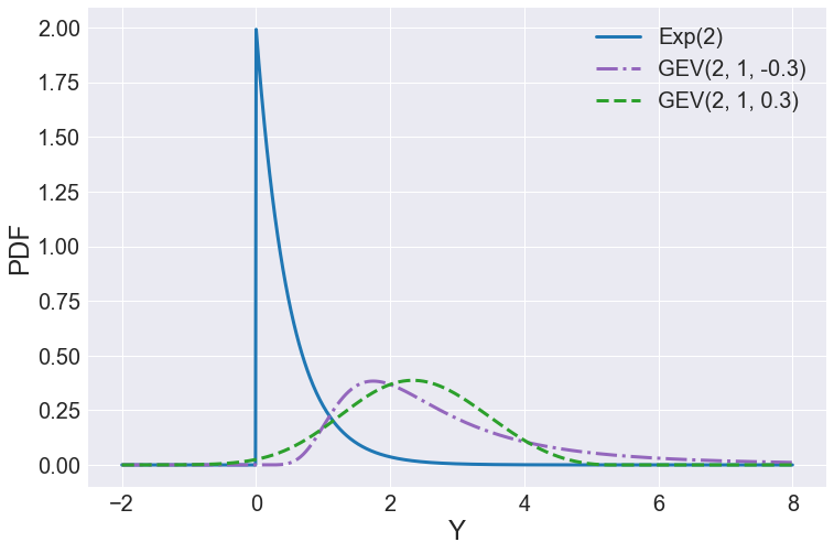
(a) PDFs

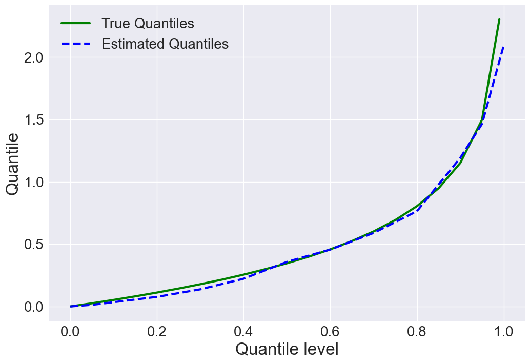
(b) Exp$(2)$

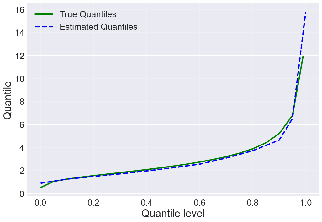
(c) GEV$(2,1,-0.3)$

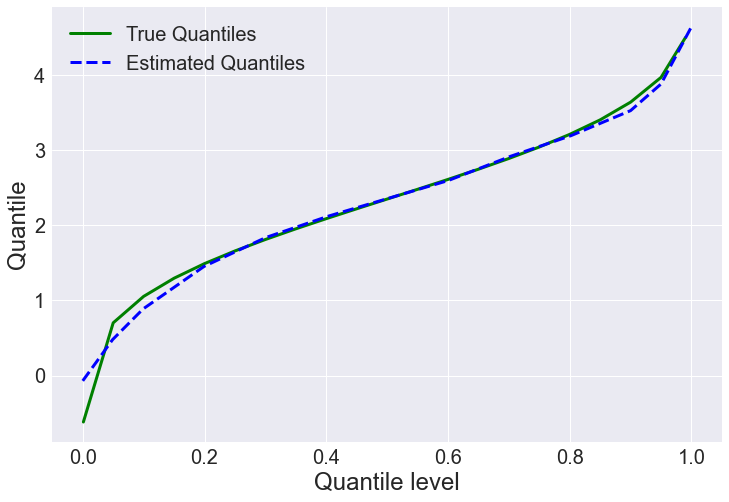
(d) GEV$(2,1,0.3)$

Figure 1: PDFs of the simulation settings (a) and quantile estimation results (b) - (d).

5.2 Robustness to distribution shift

Section 3.3 discussed the robustness of the UPR to the discrepancy between the true underlying distribution $F$ and a shifted one $Q$. A typical example of this discrepancy is a distribution shift during a test phase. To confirm the robustness, we consider a multivariate normal distribution and obtain the optimal portfolios by three models: our model (UPR) without $l_{1}$-regularization, the pessimistic portfolio model with $\alpha=0.1$ of Bassett Jr et al., (2004) (QR(0.1)) and the mean-variance model (MV). We consider three assets whose return rates are denoted by $X_{1},~{}X_{2}$, and $X_{3}$, and we postulate a distribution shift by manipulating the mean parameter of $X_{1}$ on a test phase. The distribution of the assets in a training phase is given by $(X_{1},X_{2},X_{3})^{\top}\sim F=\text{MVN}((0,0,0)^{\top},\Sigma)$, and the distribution in a test phase is given by $(X_{1},X_{2},X_{3})^{\top}\sim Q=\text{MVN}((-1,0,0)^{\top},\Sigma)$, where

$$\Sigma=\left(\begin{array}[]{ccc}0.30&0.07&0.08\\ 0.07&0.40&0.09\\ 0.08&0.09&0.50\end{array}\right).$$

Note that $\mbox{{\rm Var}}(X_{1})=0.30,\mbox{{\rm Var}}(X_{2})=0.40,\mbox{{\rm Var}}(X_{3})=0.50$ and correlation of Asset $i$ and $j$, $\rho_{ij}=0.2,~{}i\neq j.$

We fit each model with 200 random samples from $F$ and evaluate the average return rate of the optimal portfolio with 200 random samples from $Q$. This process is repeated 50 times. Table 1 summarizes the average return rates computed after 50 repeated simulations. It shows that each model assigns the largest weight to Asset 1, which also presents the smallest variance. Henceforth, Asset 1 is the most favorable asset on average under $F$. When portfolio returns follow Gaussian distribution, Bertsimas et al., (2004) showed that spectral risk measures are linear to portfolio expected return and standard deviation. Therefore, all methods allocate more weight to Asset 1 than other assets. Another important issue is that the optimal portfolio based on the UPR has smaller average weights of Asset 1 than QR(0.1) and MV. The difference in preference degree for Asset 1 is based on the difference in the distortion functions. We compare the shape of the distortion function of UPR with that of $\alpha$-risk in Supplemental material S4. For the distortion function of QR($\alpha$), $\nu_{\alpha}(t)$ only considers the $\alpha$-sized sub-population of loss. On the contrary, for the distortion function of uniform pessimistic risk, $\phi(t)$ encompasses the population’s total loss(or return) with decaying weights.

Through the former result, we found that any models prefer Asset 1 to others in $F$. In distribution $Q$, however, we change the mean of Asset 1 from $0$ to $-1$. The optimal portfolio models under $F$ could incur a larger loss as the most favorable asset becomes adverse. It is that we compel the portfolio models to confront the worse scenarios. The average returns of UPR, QR(0.1), and MV are $-0.411,-0.436$, and $-0.442$ respectively. Additionally, transitions of mean returns under the methods are presented in Figure 2 when $F$ goes to $Q$. The UPR yields smaller losses and standard errors as compared to others. That is, our proposed model has the robustness to distribution shift, which incurs the worse scenario.

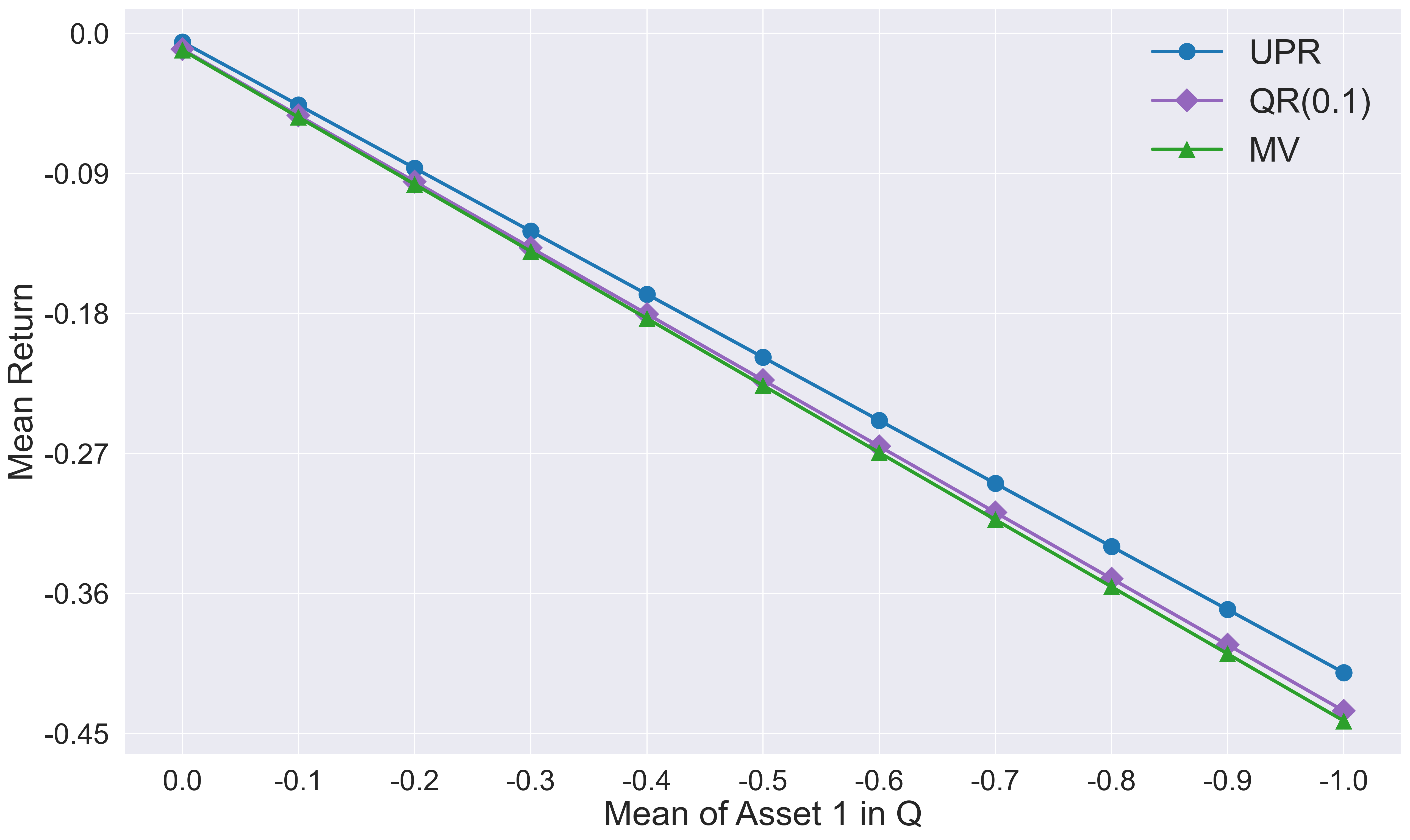
Figure 2: Mean returns of portfolio models with varying mean of Asset 1 in $Q$ distribution.

Table 1: Averages(standard errors) of weights, $\varrho_{\mbox{emp}}$ under $F$, and returns under $Q$ of the portfolio models. $\varrho_{\mbox{emp}}$ is an empirical version of the UPR. The detail of the $\varrho_{\mbox{emp}}$ is discussed in Section 5.3, real data analysis.

Model	Asset 1	Asset 2	Asset 3	$\varrho_{\mbox{emp}}$	Return($Q$)
UPR	0.405(0.404)	0.295(0.461)	0.300(0.464)	0.614(0.247)	-0.411(0.565)
QR(0.1)	0.425(0.579)	0.323(0.661)	0.252(0.509)	0.698(0.354)	-0.436(0.618)
MV	0.431(0.576)	0.315(0.662)	0.254(0.498)	0.697(0.352)	-0.442(0.614)

5.3 Real data analysis: Out-of-sample performance

We use the KOSPI200 dataset of daily log return rates of 162 assets from 2010 to 2018. The log return rates are computed with the adjusted closing stock price. To evaluate the performance of an optimal portfolio, we consider UPR, $\alpha$-risk, and Sharpe ratio (Sharpe,, 1994). All measures are computed with adjusted stock prices in the evaluation period. To explain the empirical UPR, we introduce new notations. Let $y_{i}$ for $i=1,\cdots,m$ be the logarithmic return rates and denote its empirical CDF by $F_{m}(y_{i})$. Let $\phi(j/m)=\frac{\log j/m}{\sum_{k=1}^{m}\log k/m}$ for $k=1,\cdots,m$ be a discrete distortion measure. Then, the empirical UPR is given by $\varrho_{\text{emp}}=-\sum_{j=1}^{m}F^{-1}(j/m)\phi(j/m).$ Note that $F^{-1}(j/m)=y_{(j)}$, where $y_{(j)}$ is the $j$th smallest element among $y_{i}$s. Thus,

$$\varrho_{\text{emp}}=-\sum_{j=1}^{m}y_{(j)}\phi(j/m).$$

The distortion measure satisfies the conditions of positivity and decreasing property for the admissible risk spectrum (Acerbi,, 2002). As such, $\varrho_{\text{emp}}$ is a coherent risk measure. The empirical version of $\alpha$-risk is similarly defined as the UPR. The empirical Sharpe ratio is computed by realized return rate and variance in the evaluation period.

To measure the out-of-sample performance, we consider the rolling sample estimation (DeMiguel et al., 2009b, ). Each optimal portfolio is estimated with the daily log return rates from the previous three quarters in the training time window, and daily returns of the optimal portfolio are computed in the next single quarter of the evaluation time window. Then, the quarterly return and the associated risk are obtained by the daily returns. The estimation and evaluation time windows are shifted to the next quarter forward three months, and the estimation and evaluation are repeated. By this rolling sample estimation, the portfolio performances are evaluated.

We compare the out-of-sample performances of our model with those of three benchmark models; simple quantile regression model (Bassett Jr et al.,, 2004), composite quantile regression model (4), and the mean-variance model (Markowitz,, 1952). Note that our model minimizes the UPR; the simple quantile regression minimizes the $\alpha$-risk; the composite quantile regression model minimizes the generalized pessimistic risk defined in Proposition 2; and the mean-variance model reduces the variance of the portfolio. “UPR”, “UPR($\lambda=0.01$)”, “QR($0.1$),” “CQR” and “MV” denote the UPR portfolio model without and with lasso regularization, quantile regression model at 10% quantile level, the composite quantile regression model, and the mean-variance model, respectively.

Table 2: Averages of risks and ranks over all periods of UPR portfolio models and benchmark models

Measure	UPR	UPR($\lambda=0.01$)	QR(0.1)	CQR	MV
$\varrho_{\text{emp}}$	0.0148(2.5)	0.0141(2.22)	0.0207(4.53)	0.0172(3.16)	0.0166(2.59)
$\alpha(0.1)$	0.0319(2.66)	0.0307(2.22)	0.0433(4.53)	0.0362(3.06)	0.0347(2.53)
Return	0.0012(2.59)	0.0012(2.59)	0.0004(3.44)	0.0006(3.13)	0.0006(3.25)
Sharpe ratio	0.0597(2.78)	0.0805(2.97)	0.0270(3.34)	0.0461(2.93)	0.0442(2.97)

Table 2 presents averages of measures and ranks for overall evaluation. The optimal portfolios based on UPR have a higher return and lower risk than other models. UPR($\lambda=0.01$) selects 122.6 assets on average over 162 assets. The optimal selection improves the out-of-sample performance. Our proposed methods have high-ranking, and they surpass the other methods. Figure 3 presents the results of out-of-sample performance. It can be inferred from figure that UPR($\lambda=0.01$) is the best in terms of $\varrho_{\text{emp}}$ and $\alpha(0.1)$. UPR($\lambda=0.01$) shows the best performance 15, 14 times out of 32 forecasting periods in terms of $\varrho_{\text{emp}}$ and $\alpha(0.1)$-risk. In the $29^{\small\text{th}}$ evaluation step between 2018 and 2019, the risks under other methods sharply increase. The extreme risk is not remarkably identified in the results of the Sharpe ratio. But it could incur an extreme loss for investors. In contrast, our proposed models are more risk-free in extreme situations in out-of-sample performance. Results of quantile estimation are appended in Supplemental material S5.

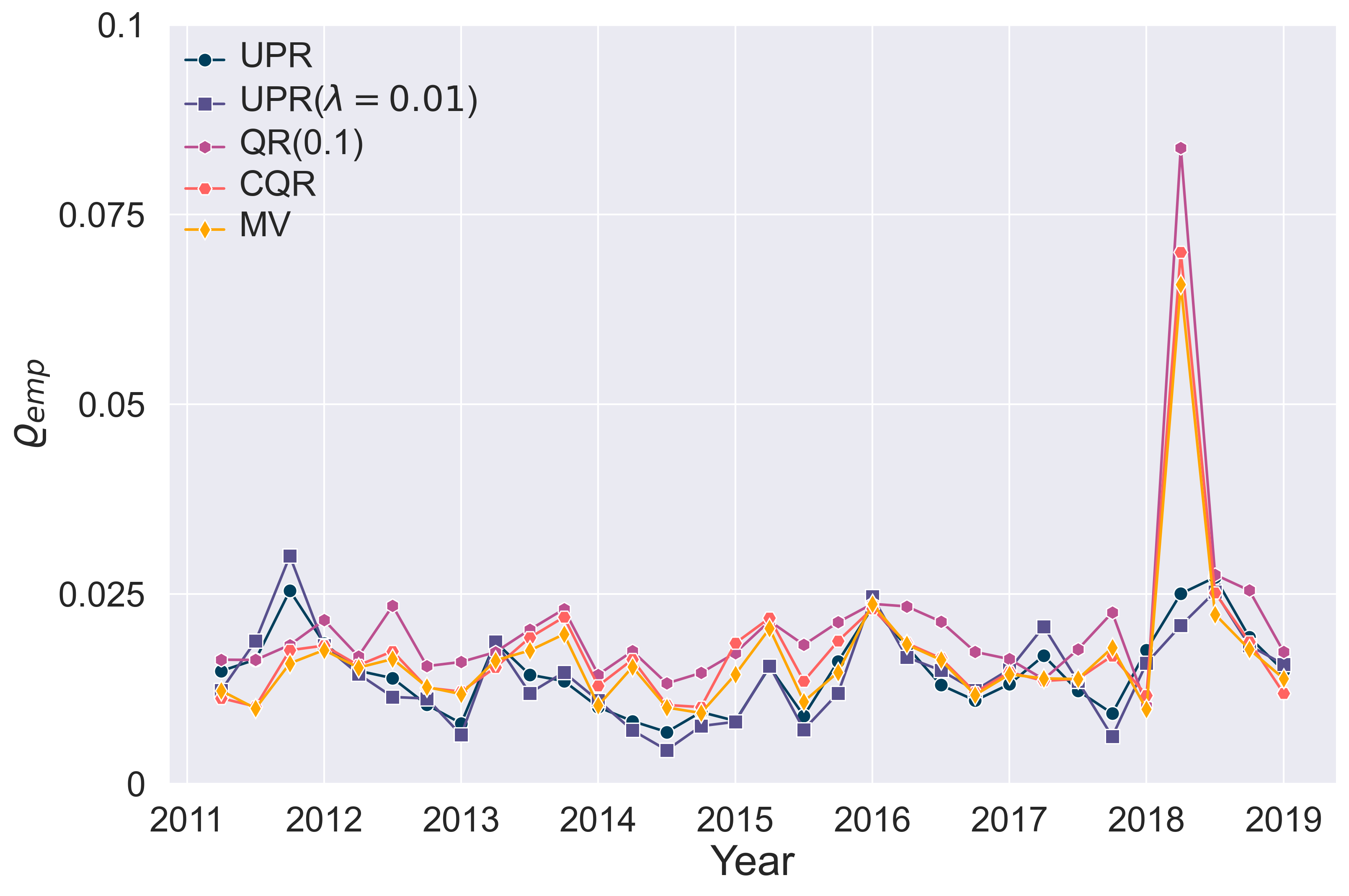
(a) Empirical UPR

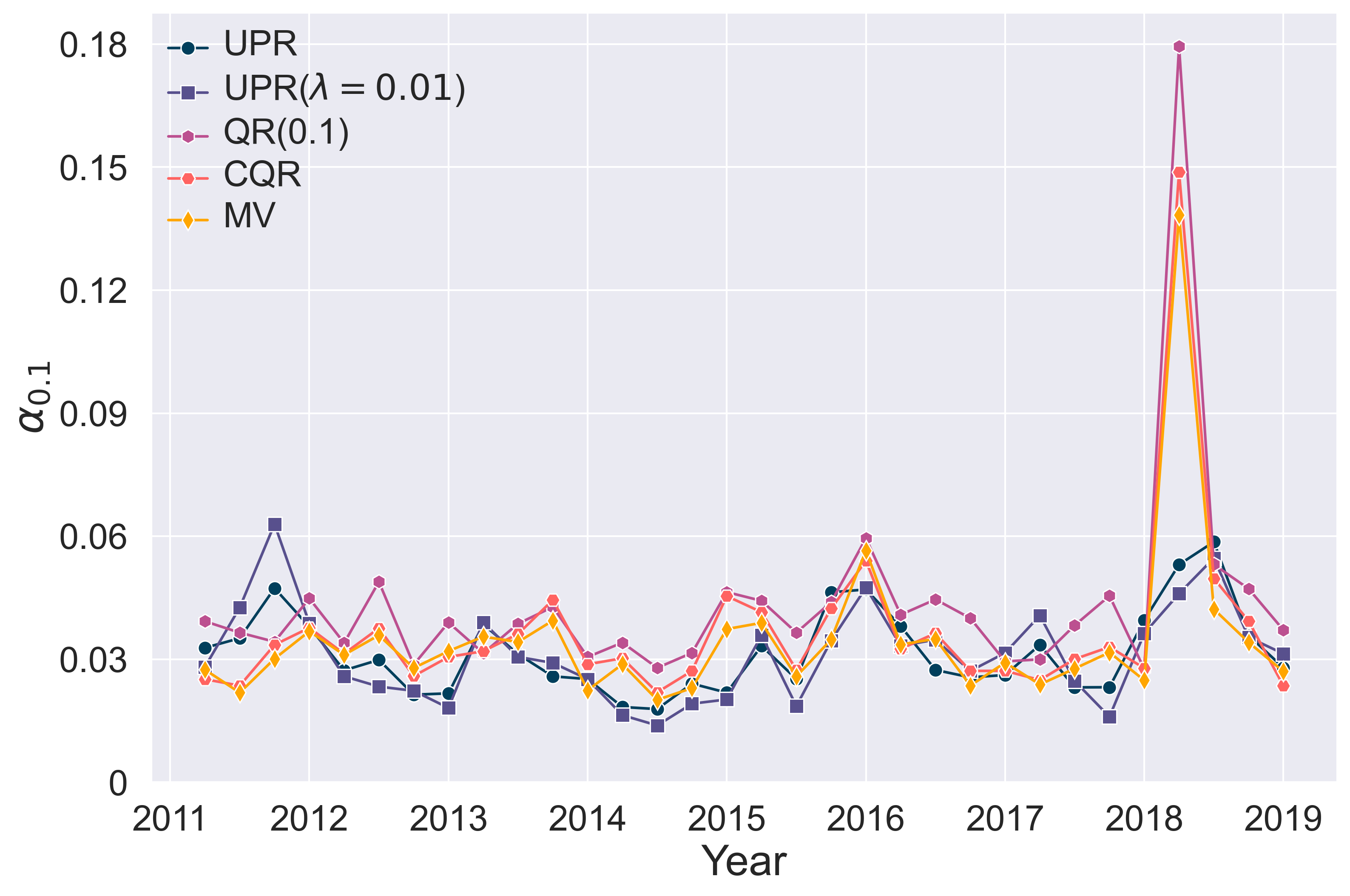
(b) $\alpha(0.1)$-risk

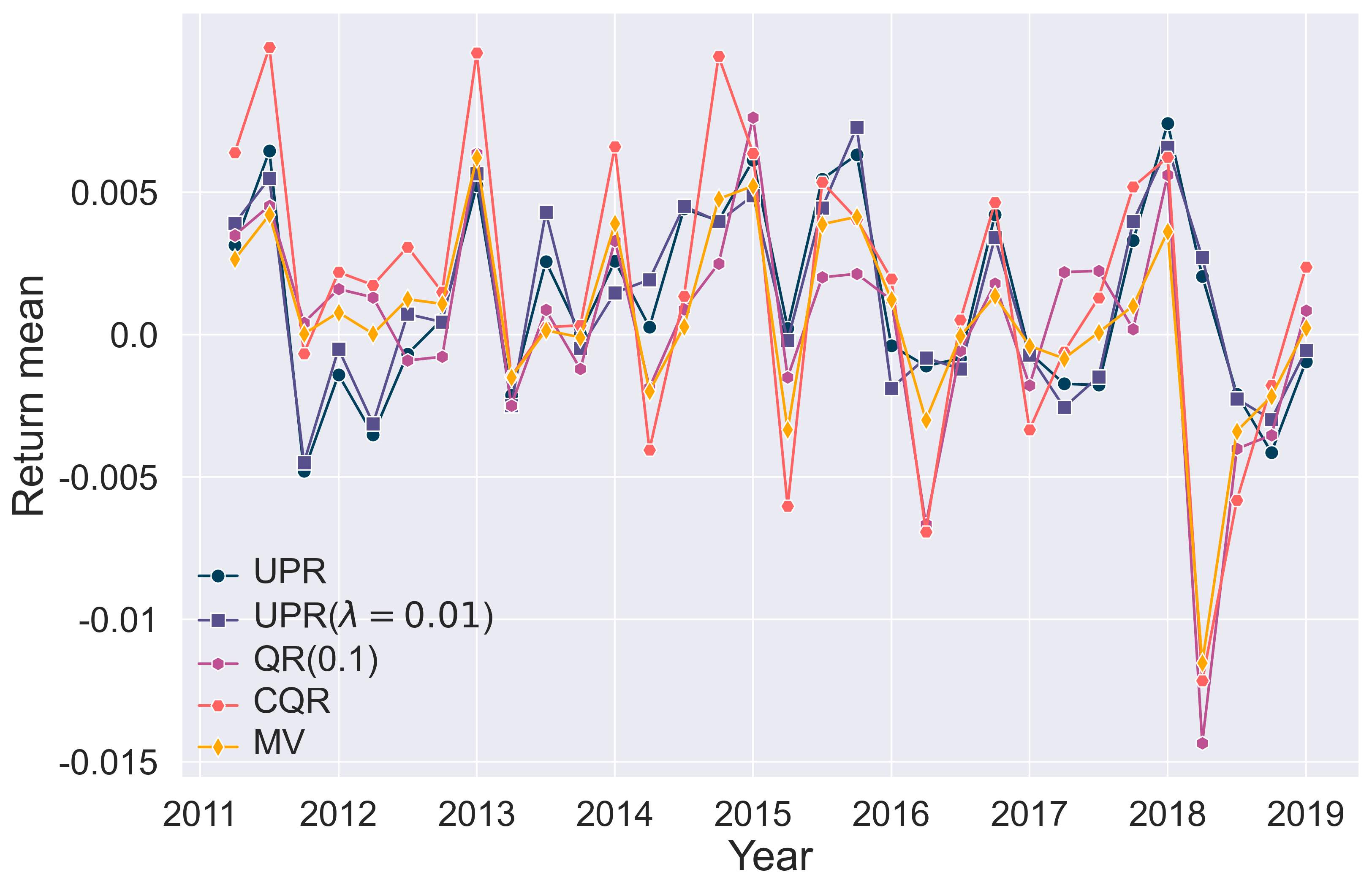
(c) Return mean

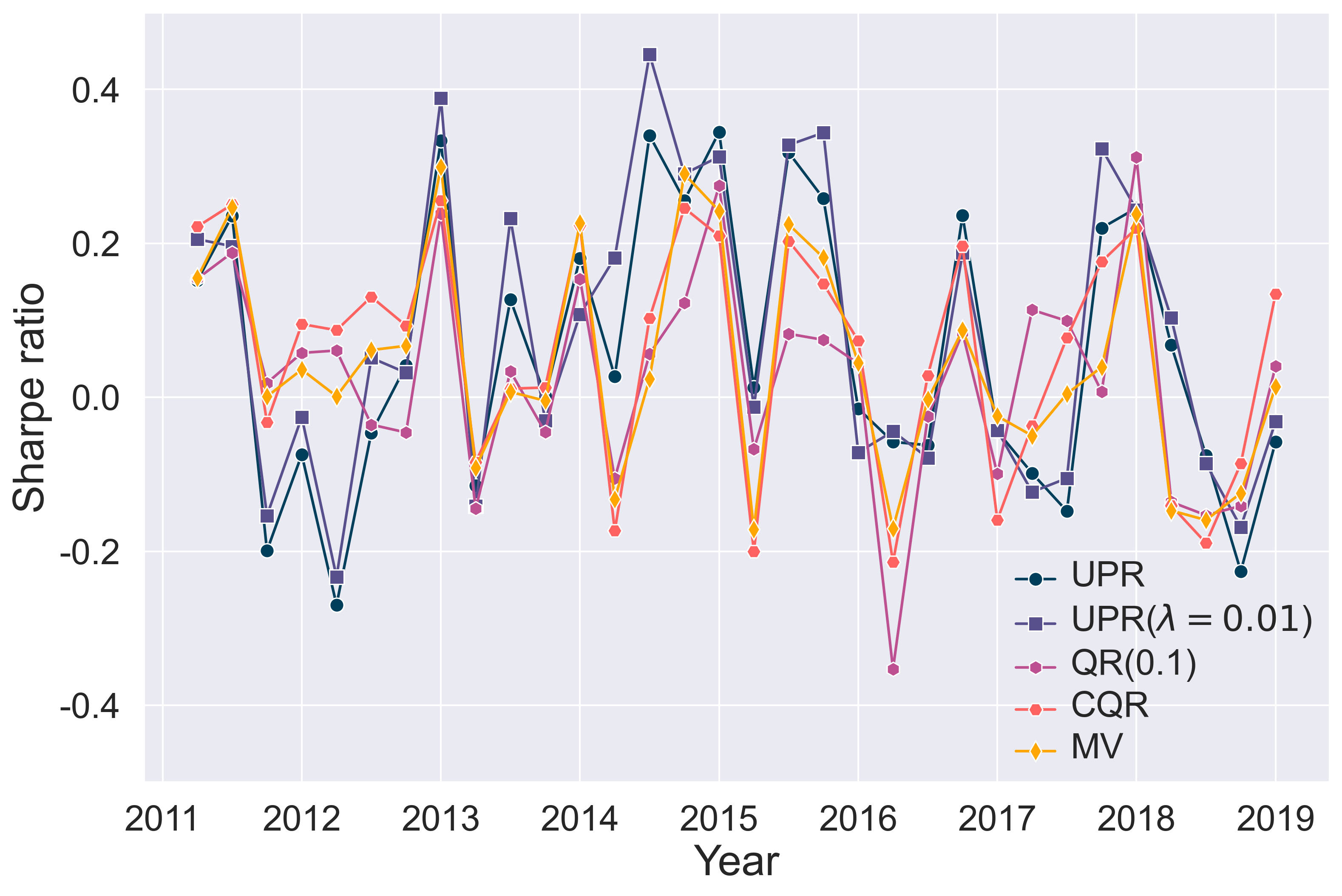
(d) Sharpe ratio

Figure 3: Out-of-sample performance of UPR portfolio models and benchmark models. All measures are calculated empirically.

We conduct data analysis to investigate the out-of-sample performance. Let $X^{\text{in}}_{i,r}$ and $X^{\text{out}}_{i,r}$ denote the in-sample and out-of-sample of $i$th asset in $r$th rolling period, $i=1,\dots 162$ and $r=1,\dots,32$. We evaluate the difference of sample mean ($\bar{X}^{\text{in}}_{i,r}-\bar{X}^{\text{out}}_{i,r}$) and standard error ($\text{se}(X^{\text{in}}_{i,r})-\text{se}(X^{\text{out}}_{i,r})$) between in-sample and out-of-sample so that we roughly detect distribution shift. Figure 4 represents the difference in statistics between the in-sample and out-of-sample of each asset. In the $29^{\small\text{th}}$ rolling period, the glaring difference in SE is detected in a specific asset. This shift produces the discrepancy of in-sample and out-of-sample and extreme loss in CQR, QR(0.1), and MV methods.

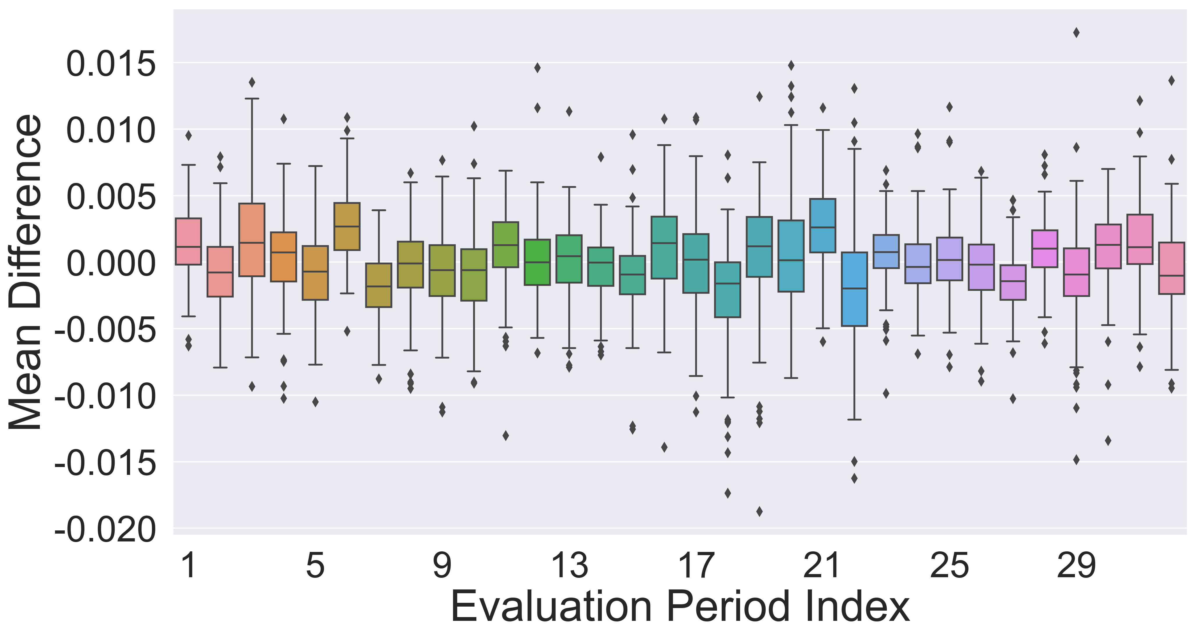
(a) Mean

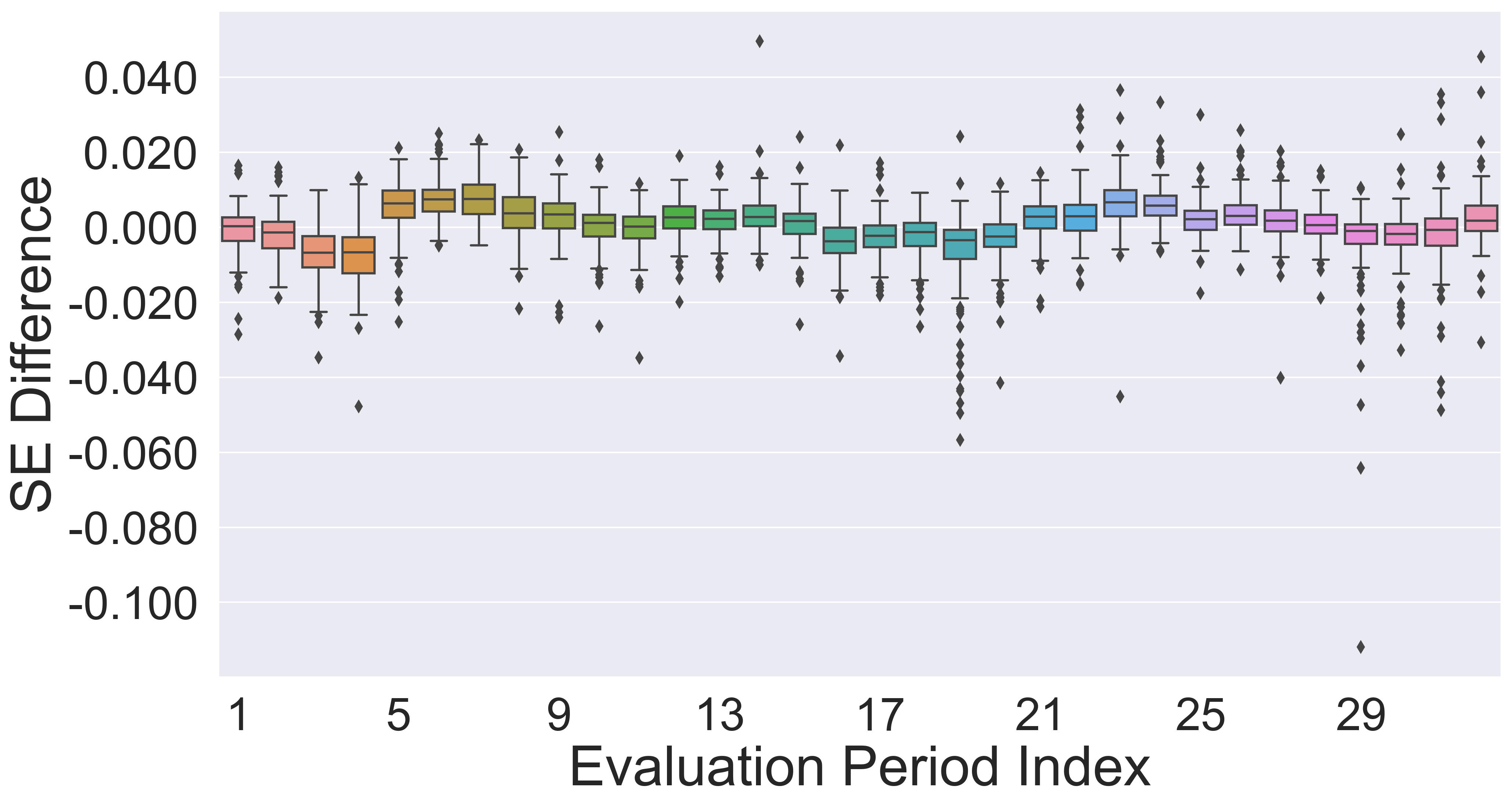
(b) Standard error (SE)

Figure 4: Boxplots of difference of statistics, mean (left), and standard error (right) between in-sample and out-of-sample of each asset.

In real data analysis, we can estimate $g_{\theta}$ of portfolio returns by using a linear isotonic regression spline. In UPR and UPR($\lambda=0.01$) cases, the estimated quantile functions are compared with empirical quantile estimates of in-sample and out-of-sample.

First, we investigate the $29^{\small\text{th}}$ evaluation period when tough losses are incurred. Figure 5 presents quantile estimation results of portfolio models: UPR, UPR($\lambda=0.01$), and CQR in the $29^{\small\text{th}}$ evaluation period. The dashed and solid lines present the estimated and empirical quantile functions of the in-sample, respectively. The dotted line presents the empirical quantiles of out-of-sample. All models have significant discrepancies between in-sample and out-of-sample quantiles in this period. Nevertheless, our proposed models have better performances of quantile estimation in in-sample and a short range of portfolio return than CQR.

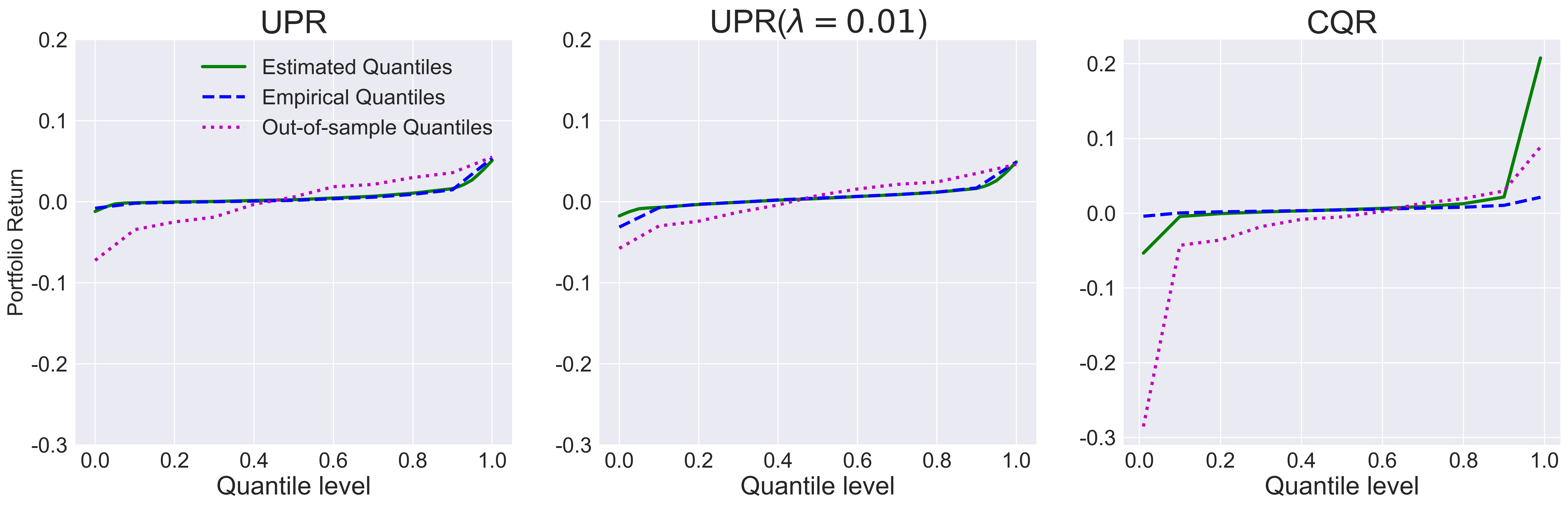
Figure 5: Quantile estimation results of UPR (left), UPR($\lambda=0.01$) (middle), CQR (right) portfolio models in $29^{\small\text{th}}$ evaluation period.

6 Concluding Remarks

In this work, we analyze three types of representation of the pessimistic risk. Based on the work of Bassett Jr et al., (2004), we derive a closed form of the general pessimistic risk, enabling the computation of the risk with a composite quantile regression model. When the expected return rate of the portfolio is fixed, the optimality based on the general pessimistic risk is equally induced by minimizing the composite quantile risk of which corresponding weights are correctly given.

The relation between the pessimistic risk and the composite quantile risk still holds even when the number of quantiles goes to infinity. As a result, we can extend the pessimistic risk with a continuous distortion measure and show that the UPR is a limit of the composite quantile risk computed by minimizing the proper score. The monotone spline regression model Gasthaus et al., (2019) derives the closed form of the UPR, and the evaluation and optimization problems for the portfolio allocation are easily solved.

In addition, the UPR is represented by the worst-case expectation. A dual representation of the convex coherent risk shows that the UPR is the worst-case expected portfolio loss when the underlying distributions of individual return rates are shifted. Thus, the optimality of the UPR implies the distributional robustness of the optimal portfolio. The real data analysis of KOSPI200 accounts for the superiority of the optimal portfolio based on the UPR partly by the robustness.

Our work leaves two interesting questions for future research. Sections 3.4 and 3.5 show that the uniform measure used in the UPR guarantees distributional robustness against distribution shift. Nevertheless, it is still unclear whether we can define an optimal selection of a distortion function in terms of robustness against the worst-case loss. One possible solution is the extension of the distortion measures by the beta distribution. Because the pessimistic risk with the beta distribution has a closed form, the class of beta mixture distribution is adequate for the extension of UPR with regard to the richness of the distribution class and the easiness of computation of the pessimistic risk. Second, we do not provide an asymptotic theory of the estimated portfolio. A semiparametric estimation theory can prove the asymptotic properties of the proposed estimator. We leave these two problems as our future work.

S1 Proofs of Propositions and Theorems

S1.1 Proof of Proposition 1

Proof.

Let $\ell_{\alpha}(z)=(\alpha-I(z<0))z$, then

$$\mbox{{\rm E}}(\ell_{\alpha}(Y-\beta_{0})) = \mbox{{\rm E}}((\alpha-I(Y-\beta_{0}<0))(Y-\beta_{0}))$$ (14)

$$= \alpha(\mbox{{\rm E}}(Y)-\beta_{0})-\int^{\beta_{0}}_{-\infty}(y-\beta_{0})dF(y)$$

$$= \alpha\mbox{{\rm E}}(Y)-\alpha\beta_{0}-\int_{-\infty}^{\beta_{0}}ydF(y)+\beta_{0}F(\beta_{0})$$

$$= \alpha\mbox{{\rm E}}(Y)-\int_{0}^{F(\beta_{0})}G(t)dt+\beta_{0}(F(\beta_{0})-\alpha).$$

Because $\underset{\beta_{0}}{\mbox{min}}~{}\mbox{{\rm E}}(\ell_{\alpha}(Y-\beta_{0}))=\mbox{{\rm E}}(\ell_{\alpha}(Y-G(\alpha))$, plugging $G(\alpha)$ into $\beta_{0}$ in (14) leads to

$$\underset{\beta_{0}}{\min}~{}\mbox{{\rm E}}(\ell_{\alpha}(Y-\beta_{0})) = \alpha\mbox{{\rm E}}(Y)-\int_{0}^{\alpha}G(t)dt$$

$$= \alpha(\mu_{0}+\varrho_{\alpha}(Y)).$$

$\square$

S1.2 Proof of Proposition 2

Proof.

For given $\{\alpha_{k}\}_{k=1,\dots,K}$, let $\beta_{k0}^{*}$ be the minimizer of $\mbox{{\rm E}}(\ell_{\alpha_{k}}(Y-\beta_{k0}))$ with respect to $\beta_{k0}$ for $k=1,\cdots,K.$ Then,

$$\varrho(Y;\varphi_{d})+\mbox{{\rm E}}(Y) = \sum_{k=1}^{K}w_{k}\left(\varrho_{\nu_{\alpha_{k}}}(Y)+\mbox{{\rm E}}(Y)\right)$$

$$= \sum_{k=1}^{K}\frac{w_{k}}{\alpha_{k}}\mbox{{\rm E}}(\ell_{\alpha_{k}}(Y-{\beta}_{k0}^{*}))$$

$$= \sum_{k=1}^{K}w^{\ast}_{k}\mbox{{\rm E}}(\ell_{\alpha_{k}}(Y-{\beta}_{k0}^{*}))$$

where $w^{\ast}_{k}=w_{k}/\alpha_{k}$. The second equality holds by Proposition 1. $\square$

S1.3 Proof of Proposition 3

Proof.

Denote the probability density function of $Y$ by $f(\cdot)$. By change of variables with $G(\alpha)=t$, we can rewrite $\varrho(Y;\varphi_{u})$ as follows:

$$\varrho(Y;\varphi_{u}) = -\int_{0}^{1}\frac{1}{\alpha}\int_{0}^{\alpha}G(t)dtd\alpha$$

$$= -\int_{0}^{1}\int_{-\infty}^{G(\alpha)}\frac{1}{\alpha}yf(y)dyd\alpha$$

$$= -\int_{-\infty}^{\infty}\int_{-\infty}^{t}\frac{1}{F(t)}yf(y)f(t)dydt$$

$$= -\int_{-\infty}^{\infty}yf(y)\left[\log F(t)\right]_{t=y}^{\infty}dy=\int_{-\infty}^{\infty}yf(y)\log F(y)dy.$$

By Fubini’s theorem the third equality above holds whenever $\int_{-\infty}^{\infty}|yf(y)\log F(y)|dy<\infty$, which is guaranteed by Assumption A. Thus, the exchange of double integrals in $\varrho(Y;\varphi_{u})$ leads to

$$\varrho(Y;\varphi_{u}) = -\int^{1}_{0}\frac{1}{\alpha}\int_{0}^{\alpha}G(t)dtd\alpha$$

$$= -\int_{0}^{1}G(t)\int_{t}^{1}\frac{1}{\alpha}d\alpha dt$$

$$= -\int_{0}^{1}G(t)(-\log t)dt.$$

$\square$

S1.4 Proof of Proposition 5

Proof.

$\mathcal{R}(G,G)\geq 0$ is trivial because $\ell_{\alpha}(Y-G(\alpha))\geq 0$ almost surely. Proposition 1 implies that $\int_{0}^{1}\left(\varrho_{\alpha}(Y)+\mbox{{\rm E}}(Y)\right)d\alpha=\int_{0}^{1}\alpha^{-1}\mbox{{\rm E}}(\ell_{\alpha}(Y-G(\alpha)))d\alpha=\mathcal{R}(G,G)$, which concludes $\mathcal{R}(G,G)<\infty$ by Proposition 3.

From Proposition 1, we have $\mbox{{\rm E}}[\ell_{\alpha}(Y-G(\alpha))]\leq\mbox{{\rm E}}[\ell_{\alpha}(Y-g(\alpha))]$ for any $g$. Therefore,

$$\mathcal{R}(G,G)-\mathcal{R}(g,G)$$

$$= \int_{0}^{1}\left(\frac{1}{\alpha}\mbox{{\rm E}}\left[\ell_{\alpha}(Y-G(\alpha))\right]-\frac{1}{\alpha}\mbox{{\rm E}}[\ell_{\alpha}(Y-g(\alpha))]\right)d\alpha$$

$$\leq 0,$$

then $0\leq\mathcal{R}(G,G)\leq\mathcal{R}(g,G)$.

Now we will show that $\mathcal{R}(g,G)<\infty$. Assumption A and the assumption of proposition 5 imply that

$$|F(g(\alpha))g(\alpha)|\asymp|\alpha^{-q}|^{-r}(\alpha^{-q})=\alpha^{q(r-1)}$$

for some $r>1$ ane $0<q<1$ as $\alpha\downarrow 0$. Because $|F(g(\alpha))g(\alpha)|\asymp\alpha^{q(r-1)}$ with $q(r-1)>0$ as $\alpha\downarrow 0$ and $\int_{0}^{1}|g(\alpha)|d\alpha<\infty$,

$$\left|\int_{0}^{1}\frac{1}{\alpha}F(g(\alpha))g(\alpha)d\alpha\right|<\infty.$$ (15)

Similarly, it is shown that $\int_{-\infty}^{g(\alpha)}ydF(y)\asymp\alpha^{q(r-1)}$ as $\alpha\downarrow 0$, which implies

$$\left|\int_{0}^{1}\frac{1}{\alpha}\int_{-\infty}^{g(\alpha)}ydF(y)\right|<\infty$$ (16)

with $\mbox{{\rm E}}(Y)<\infty$. Then,

$$\mathcal{R}(g,G) = \int_{0}^{1}\frac{1}{\alpha}\mbox{{\rm E}}\left[\ell_{\alpha}(Y-g(\alpha))\right]d\alpha$$

$$= \int_{0}^{1}\frac{1}{\alpha}\left[\int_{-\infty}^{\infty}(\alpha-I(y\leq g(\alpha)))(y-g(\alpha))dF(y)\right]d\alpha$$

$$= \int_{0}^{1}\frac{1}{\alpha}\left[\int_{-\infty}^{\infty}\alpha y-\alpha g(\alpha)+g(\alpha)I(y\leq g(\alpha))-yI(y\leq g(\alpha))dF(y)\right]d\alpha$$

$$= \int_{0}^{1}\frac{1}{\alpha}\left[\alpha\mbox{{\rm E}}(Y)-\alpha g(\alpha)+g(\alpha)F(g(\alpha))-\int_{-\infty}^{g(\alpha)}ydF(y)\right]d\alpha$$

$$= \mbox{{\rm E}}(Y)-\int_{0}^{1}g(\alpha)d\alpha+\int_{0}^{1}\frac{1}{\alpha}F(g(\alpha))g(\alpha)d\alpha-\int_{0}^{1}\frac{1}{\alpha}\int_{-\infty}^{g(\alpha)}ydF(y)d\alpha$$

$$< \infty.$$

The last equality holds because $\mbox{{\rm E}}|Y|<\infty$, $\int_{0}^{1}|g(\alpha)|d\alpha<\infty$, (15), and (16). $\square$

S1.5 Proof of Proposition 6

Proof.

By Proposition 5, $R(G,G)<\infty$ and

$$\mathcal{R}(G,G)-\mathcal{R}(g,G)$$ (17)

$$= \int_{0}^{1}\frac{1}{\alpha}\mbox{{\rm E}}\left[\ell_{\alpha}(Y-G(\alpha))\right]-\frac{1}{\alpha}\mbox{{\rm E}}[\ell_{\alpha}(Y-g(\alpha))]d\alpha$$

$$= \int_{0}^{1}\bigg{[}g(\alpha)-G(\alpha)+\frac{1}{\alpha}\int y(I(y\leq g(\alpha))-I(y\leq G(\alpha)))$$

$$~{}~{}~{}~{}~{}~{}~{}~{}~{}~{}~{}~{}~{}~{}~{}~{}~{}~{}~{}~{}~{}~{}~{}~{}~{}~{}~{}~{}~{}~{}~{}~{}~{}+I(y\leq G(\alpha))G(\alpha)-I(y\leq g(\alpha))g(\alpha)dF(y)\bigg{]}d\alpha.$$

Let the integrand of (17) be $D(\alpha;g,G)$, and then it suffices to prove that $\int_{0}^{1}D(\alpha;g,G)d\alpha=-\infty$ for an arbitrary continuous, bounded, and non-decreasing function $g_{\theta}$.
Define a function $m:(0,1)\mapsto\mathbb{R}$ satisfying

$$\min(g(\alpha),G(\alpha))\leq m(\alpha)\leq\max(g(\alpha),G(\alpha)).$$

Then, it follows that

$$\int y\big{(}I(y\leq g(\alpha))-I(y\leq G(\alpha))\big{)}dF(y)$$ (18)

$$\leq \int m(\alpha)\big{(}I(y\leq g(\alpha))-I(y\leq G(\alpha))\big{)}dF(y).$$ (19)

By replacing the term (18) in $D(\alpha;g,G)$ by (19), we obtain for all $\alpha\in(0,1)$

$$D(\alpha;g,G) \leq g(\alpha)-G(\alpha)+\frac{1}{\alpha}\int\bigg{[}m(\alpha)(I(y\leq g(\alpha))-I(y\leq G(\alpha)))$$ (20)

$$~{}~{}~{}~{}~{}~{}~{}~{}~{}~{}~{}~{}~{}~{}~{}~{}~{}~{}~{}~{}~{}~{}~{}~{}~{}~{}+I(y\leq G(\alpha))G(\alpha)-I(y\leq g(\alpha))g(\alpha)\bigg{]}dF(y)$$

$$= g(\alpha)-G(\alpha)+\frac{1}{\alpha}\bigg{[}m(\alpha)(F(g(\alpha))-\alpha)+\alpha G(\alpha)-F(g(\alpha))g(\alpha)\bigg{]}$$

$$= (g(\alpha)-m(\alpha))\left(1-\frac{F(g(\alpha))}{\alpha}\right)=D^{*}(\alpha;g,G).$$

$g:(0,1)\mapsto\mathbb{R}$ is a continuous, bounded, and non-decreasing function, and we can set $x_{1}\in\mathbb{R}$ and $\alpha_{1}\in(0,1)$ such that $g(\alpha)=x_{1}$ for all $0<\alpha\leq\alpha_{1}$. While, $G(\alpha)$ is unbounded, non-decreasing function, we can set $\alpha_{1}^{\prime}$ such that $G(\alpha)\leq x_{1}-\epsilon$ for $0<\alpha\leq\alpha_{1}^{\prime}$. Let $\alpha_{L}=\min(\alpha_{1},\alpha_{1}^{\prime})$. Then, by definition of $m(\alpha)$, we can choose the $m(\cdot)$ satisfying $m(\alpha)=x_{1}-\epsilon/2$ for $0<\alpha\leq\alpha_{L}$, which implies $g(\alpha)-m(\alpha)=\epsilon/2$ for $\alpha\in(0,\alpha_{L})$. Similarly, we can set $\alpha_{U}\in(\alpha_{L},1)$, such that $g(\alpha)-m(\alpha)=-\epsilon/2$. Because $g(\cdot)$ and $G(\cdot)$ is continuous, $g(\alpha)-m(\alpha)$ is bounded on $[\alpha_{L},\alpha_{U}]$. Thus, without loss of generality, we can assume that $g(\alpha)-m(\alpha)$ is bounded.

Here, it is shown that $\int_{0}^{\alpha_{L}}D^{*}(\alpha;g,G)d\alpha=-\infty$, since $\underset{\alpha\downarrow 0}{\lim}~{}F(g(\alpha))=F(x_{1})>0$. Because $\int_{\alpha_{L}}^{1}D^{*}(\alpha;g,G)d\alpha<\infty$, we can conclude that $\int_{0}^{1}D^{*}(\alpha;g,G)d\alpha=-\infty$, which completes the proof. $\square$

S1.6 Proof of Lemma 1

Proof.

Firstly, we induce a lower bound of $D(\alpha;g,G)$. Consider two cases as follows:

1. $g(\alpha)\geq G(\alpha)$

2. $G(\alpha)>g(\alpha)$

In both cases, we obtain

$$\int G(\alpha)(I(y\leq g(\alpha))-I(y\leq G(\alpha)))dF(y)$$

$$\leq \int y(I(y\leq g(\alpha))-I(y\leq G(\alpha)))dF(y)$$

$$\leq \int g(\alpha)(I(y\leq g(\alpha))-I(y\leq G(\alpha)))dF(y).$$ (22)

By replacing (18) with (Proof.) in $D(\alpha;g,G)$ and using $D^{*}(\alpha;g,G)$, we obtain

$$\int_{\eta}^{1}(g(\alpha)-G(\alpha))\left(1-\frac{F(g(\alpha))}{\alpha}\right)d\alpha\leq\int_{\eta}^{1}D(\alpha;g,G)d\alpha\leq\int_{\eta}^{1}D^{*}(\alpha;g,G)d\alpha.$$

There is a constant $K$ such that $0<F(g(\alpha))/\alpha\leq K<\infty$ where $\alpha\in[\eta,1)$. Under Assumption B,

$$\int_{\eta}^{1}\left|g(\alpha)\frac{F(g(\alpha))}{\alpha}\right|d\alpha\leq K\int_{\eta}^{1}|g(\alpha)|d\alpha<\infty.$$

Under $\mbox{{\rm E}}|Y|<\infty$ implying $\int_{0}^{1}G(\alpha)d\alpha<\infty$, we have $\int_{\eta}^{1}|G(\alpha)|d\alpha<\infty$. Then,

$$\int_{\eta}^{1}\left|G(\alpha)\frac{F(g(\alpha))}{\alpha}\right|d\alpha<\infty.$$

Therefore, there are constants, $-\infty<M_{1}\leq M_{2}\leq 0$ such that

$$M_{1}=\int_{\eta}^{1}(g(\alpha)-G(\alpha))\left(1-\frac{F(g(\alpha))}{\alpha}\right)d\alpha\leq\int_{\eta}^{1}D(\alpha;g,G)d\alpha\leq\int_{\eta}^{1}D^{*}(\alpha;g,G)d\alpha=M_{2}.$$

Thus,

$$\left|\int_{\eta}^{1}D(\alpha;g,G)\right|<\infty,$$

which concludes $\mathcal{R}_{\eta}(g,G)<\infty$.

Because replacing the term (18) in $D(\alpha;g,G)$ with (22) leads to $\mathcal{R}_{\eta}(G,G)-\mathcal{R}_{\eta}(g,G)\leq 0$, we obtain $0\leq\mathcal{R}_{\eta}(G,G)\leq\mathcal{R}_{\eta}(g,G)<\infty$. Finally, $\underset{\eta\downarrow 0}{\lim}~{}\mathcal{R}_{\eta}(G,G)=\mathcal{R}(G,G)$ by $\mathcal{R}(G,G)<\infty$. $\square$

S1.7 Proof of Theorem 1

Proof.

By Lemma 1, $\mathcal{R}_{\eta}(g_{\theta},G)<\infty$. In addition, $\mathcal{R}_{\eta}(g_{\theta},G)=\int_{\eta}^{1}\alpha^{-1}\mbox{{\rm E}}[\ell_{\alpha}(Y-g_{\theta}(\alpha))]d\alpha=\mbox{{\rm E}}\left(\int_{\eta}^{1}\alpha^{-1}\ell_{\alpha}(Y-g_{\theta}(\alpha))d\alpha\right)$ by Fubini-Tonelli theorem, such that $E|\int_{\eta}^{1}\alpha^{-1}\ell_{\alpha}(Y-g_{\theta}(\alpha))d\alpha|<\infty$. Thus, it follows that

$$\frac{1}{n}\sum_{i=1}^{n}\int_{\eta}^{1}\alpha^{-1}\ell_{\alpha}(y_{i}-g_{\theta}(\alpha))d\alpha\rightarrow E\left(\int_{\eta}^{1}\alpha^{-1}\ell_{\alpha}(Y-g_{\theta}(\alpha))d\alpha\right)$$

almost surely as $n\rightarrow\infty$ by the law of large numbers. $\square$

S1.8 Proof of Theorem 2

Proof.

Let $S_{\eta}(\theta,y)=\int_{\eta}^{1}\alpha^{-1}\ell_{\alpha}(y-g_{\theta}(\alpha))d\alpha$. Suppose that the following conditions hold:

1. For each $\theta\in\Theta$ there exist $\omega:[\eta,1)\rightarrow\mathbb{R}$, and a small neighborhood $U$ of $\theta$ such that $\underset{\theta\in U}{\sup}\frac{1}{\alpha}|g_{\theta}(\alpha)|\leq\omega(\alpha)$ and $\int_{\eta}^{1}|\omega(\alpha)|d\alpha<\infty$.

2. For a sequence $\theta_{n}$ going to $\theta$, a pointwise limit $g_{\theta}(\alpha)=\underset{\theta_{n}\rightarrow\theta}{\lim}g_{\theta_{n}}(\alpha)$ exists.

$$|S_{\eta}(\theta_{n},y)-S_{\eta}(\theta,y)| = \Big{|}\int_{\eta}^{1}\alpha^{-1}\left(\ell_{\alpha}(y-g_{\theta_{n}}(\alpha))-\ell_{\alpha}(y-g_{\theta}(\alpha))\right)d\alpha\Big{|}$$

$$= \Big{|}\int_{\eta}^{1}\alpha^{-1}\Big{[}-(\alpha-I(y\leq g_{\theta_{n}}(\alpha)))(g_{\theta_{n}}(\alpha)-g_{\theta}(\alpha))$$

$$+ \int_{0}^{G_{\theta_{n}}(\alpha)-G_{\theta}(\alpha)}I(y\leq g_{\theta_{n}}(\alpha)+s)-I(y\leq g_{\theta_{n}}(\alpha))ds\Big{]}d\alpha\Big{|}$$

$$\leq 2\int_{\eta}^{1}\alpha^{-1}|(g_{\theta_{n}}(\alpha)-g_{\theta}(\alpha))|d\alpha,$$

where the second equality follows from Knight’s identity.
Because $\alpha^{-1}|g_{\theta_{n}}(\alpha)-g_{\theta}(\alpha)|$ is bounded from above by $2\omega(\alpha)$,

$$\underset{\theta_{n}\rightarrow\theta}{\lim}\int_{\eta}^{1}\alpha^{-1}|(g_{\theta_{n}}(\alpha)-g_{\theta}(\alpha))|d\alpha=\int_{\eta}^{1}\alpha^{-1}|\underset{\theta_{n}\rightarrow\theta}{\lim}(g_{\theta_{n}}(\alpha)-g_{\theta}(\alpha))|d\alpha=0$$

by dominated convergence theorem. Thus, $S_{\eta}(\theta,y)$ is continuous at $\theta$. Then, by theorem 5.14(Van der Vaart,, 2000),

$$\Pr\left(d(\hat{\theta}_{n},\Theta_{0})>\epsilon,\hat{\theta}_{n}\in\Theta\right)\rightarrow 0$$

as $n\rightarrow\infty$. $\square$

S1.9 Proof of Theorem 3

Proof.

We introduce a beta distribution as $\varphi=b(\alpha;s,h)\sim\text{Beta}(s,h)$. Suppose that $\alpha\sim b(\alpha;s,h),~{}s\geq 1$ and $h=1$ then, pessimistic risk measure $\varrho_{(s,h)}(Y)$ can be written as follows:

$$\varrho_{(s,1)}(Y) = -\int_{0}^{1}\frac{b(\alpha;s,1)}{\alpha}\int_{0}^{\alpha}G(t)dtd\alpha$$

$$= -\int_{0}^{1}\frac{1}{B(1,s,1)}\alpha^{s-2}\int_{-\infty}^{G(\alpha)}yf(y)dyd\alpha$$

$$= -s\int_{0}^{1}\int_{-\infty}^{t}F(t)^{s-2}yf(y)f(t)dydt$$

$$= -s\int_{-\infty}^{\infty}yf(y)\int_{y}^{\infty}F(t)^{s-2}f(t)dtdy$$

$$= -\frac{s}{s-1}\int_{-\infty}^{\infty}yf(y)(1-F(y)^{s-1})dy,$$

where $s\neq 1$.
Under Assumption A, $\int_{-\infty}^{\infty}|yf(y)(1-F(y)^{s-1})|dy<\infty$. Therefore, the exchange of double integrals leads to

$$\varrho_{(s,1)}(Y) = -\int_{0}^{1}\frac{1}{B(1,s,1)}\alpha^{s-2}\int_{0}^{\alpha}G(t)dtd\alpha=-\int_{0}^{1}s\alpha^{s-2}\int_{0}^{\alpha}G(t)dtd\alpha$$

$$= -\int_{0}^{1}G(t)s\int_{t}^{1}\alpha^{s-2}d\alpha dt$$

$$= -\int_{0}^{1}G(t)s\left[\frac{\alpha^{s-1}}{s-1}\right]_{\alpha=t}^{1}dt$$

$$= -\int_{0}^{1}\frac{s}{s-1}G(t)(1-t^{s-1})dt.$$

Let $G(t)=y$, then

$$-\int_{0}^{1}\frac{s}{s-1}G(t)(1-t^{s-1})dt = -\int_{-\infty}^{\infty}\frac{s}{s-1}y(1-\{F(y)\}^{s-1})f(y)dy$$ (23)

$$= -\int_{-\infty}^{\infty}\frac{s}{s-1}(yf(y)-y\{F(y)\}^{s-1}f(y))dy$$

$$= -\frac{s}{s-1}\left[\mbox{{\rm E}}(Y)-\mbox{{\rm E}}(Y\{F(Y)\}^{s-1})\right].$$

The cumulative distribution function and probability density function of the GEV distribution are given as follows:

$$F(y;\xi,\zeta,\kappa) = \exp\left(-\left\{1-\kappa\left(\frac{y-\xi}{\zeta}\right)\right\}^{1/\kappa}\right),$$

$$f(y;\xi,\zeta,\kappa) = \exp\left(-\left\{1-\kappa\left(\frac{y-\xi}{\zeta}\right)\right\}^{1/\kappa}\right)\frac{1}{\zeta}\left\{1-\kappa\left(\frac{x-\xi}{\zeta}\right)\right\}^{1/\kappa-1}$$

s.t. $$\kappa\neq 0~{}\text{and}~{}1-\kappa\left(\frac{y-\xi}{\zeta}\right)>0,$$

where $\xi,\zeta,$ and $\kappa$ are the location, scale, and shape parameters, respectively.

For $Y\sim\text{GEV}(\xi,\zeta,\kappa)$ with $\kappa>-1$, the probability-weighted moments (Jeon et al.,, 2011), $\mbox{{\rm E}}(Y\{F(Y)\}^{s-1})$ is written in a closed form as

$$\mbox{{\rm E}}(Y\{F(Y)\}^{s-1})=\frac{1}{s}[\xi+\zeta(1-s^{-\kappa}\Gamma(1+\kappa))/\kappa],$$

and expectation of $Y$ is $\mbox{{\rm E}}(Y)=\xi+\frac{\zeta}{\kappa}(1-\Gamma(1+\kappa))$.
Then plugging them into above equation (23),

$$\varrho_{(s,1)}(Y) = -\frac{s}{s-1}\left[\xi+\frac{\zeta}{\kappa}(1-\Gamma(1+\kappa)-\frac{1}{s}\{\xi+\zeta(1-s^{-\kappa}\Gamma(1+\kappa))/\kappa\}\right]$$ (24)

$$= \frac{\zeta\Gamma(1+\kappa)}{\kappa}\cdot\frac{(s-s^{-\kappa})}{s-1}-\xi-\frac{\zeta}{\kappa}=\frac{a}{\kappa}\cdot\frac{(s-s^{-\kappa})}{s-1}+c$$

where $a>0$ and $c$ are constants which do not depend on $s$.
Then, for $s>1$,

$$\left(\frac{s-s^{-\kappa}}{s-1}\right)^{\prime}=\frac{(\kappa+1)s^{-\kappa}-\kappa s^{-\kappa-1}-1}{(s-1)^{2}}=\begin{cases}>0,&-1<\kappa<0,\\ <0,&\kappa>0.\end{cases}$$

Now we show that $\varrho_{(s,1)}(Y)$ is right-continuous at $s=1$. Let $(1-\kappa((y-\xi)/\zeta))^{1/\kappa}=x$ then,

$$\varrho_{(1,1)}(Y) = \int y(-\log F(y))f(y)dy$$

$$= \int y\left\{1-\kappa\left(\frac{y-\xi}{\zeta}\right)\right\}^{1/\kappa}\exp\left(-\left\{1-\kappa\left(\frac{y-\xi}{\zeta}\right)\right\}^{1/\kappa}\right)\frac{1}{\zeta}\left\{1-\kappa\left(\frac{x-\xi}{\zeta}\right)\right\}^{1/\kappa-1}dy$$

$$= \int_{0}^{\infty}\zeta\left(\frac{1-x^{\kappa}}{\kappa}+\xi\right)(-x)\exp(-x)dx$$

$$= \frac{\zeta\Gamma(2+\kappa)}{\kappa}-\xi-\frac{\zeta}{\kappa},$$

and the limit of (24) as $s\downarrow 1$ is given by,

$$\lim_{s\downarrow 1}\varrho_{(s,1)}(Y) = \lim_{s\downarrow 1}\frac{s-s^{-\kappa}}{s-1}\frac{\zeta\Gamma(1+\kappa)}{\kappa}-\xi-\frac{\zeta}{\kappa}$$

$$= (\kappa+1)\frac{\zeta\Gamma(1+\kappa)}{\kappa}-\xi-\frac{\zeta}{\kappa}$$

$$= \varrho_{(1,1)}(Y).$$

Therefore, $\varrho_{(s,1)}$ is right-continuous at $s=1$ when $\kappa\neq 0$. Similarly, we can show that $\varrho_{(s,1)}$ is decreasing w.r.t $s>1$ and right-continuous at $s=1$ when $\kappa=0$, i.e., $Y$ is a Gumbel random variable. As a consequence, $\varrho_{(s,1)}(Y)$ is a monotonically decreasing function of $s$ where $s\geq 1$. $\square$

S1.10 Proof of Theorem 4

Proof.

We have

$$\int_{0}^{1}\frac{1}{\alpha}\mbox{{\rm E}}(\ell_{\alpha}(Y-g(\alpha)))b(\alpha;s,h)d\alpha$$

$$= \int_{0}^{1}\frac{b(\alpha;s,h)}{\alpha}\left[\int\alpha y-\alpha g(\alpha)+I(y\leq g(\alpha))g(\alpha)-I(y\leq g(\alpha))ydF(y)\right]d\alpha$$

$$= \mbox{{\rm E}}(Y)-\int_{0}^{1}b(\alpha;s,h)g(\alpha)d\alpha+\int_{0}^{1}\frac{b(\alpha;s,h)}{\alpha}\left(F(g(\alpha))g(\alpha)-\int_{-\infty}^{g(\alpha)}ydF(y)\right)d\alpha.$$

When $s\geq 1$ and $h\geq 1$, then $\sup_{\alpha\in(0,1)}b(\alpha;s,h)<\infty$. Because $\int_{0}^{1}|g(\alpha)|d\alpha<\infty$,

$$\int_{0}^{1}|b(\alpha;s,h)g(\alpha)|d\alpha<\infty.$$

Now we prove that

$$\left|\int_{0}^{1}\frac{b(\alpha;s,h)}{\alpha}F(g(\alpha))g(\alpha)d\alpha\right|<\infty\mbox{ and }\left|\int_{0}^{1}\frac{b(\alpha;s,h)}{\alpha}\int_{-\infty}^{g(\alpha)}ydF(y)d\alpha\right|<\infty.$$

There are two possible cases listed as follows:

1. $g$ is not bounded from below.

2. $g$ is bounded from below.

If $g$ is not bounded from below, $b(\alpha;s,h)\int_{-\infty}^{g(\alpha)}ydF(y)\asymp\alpha^{(s-1)+q(r-1)}$ as $\alpha\downarrow 0$ for $s\geq 1$, $0<q<1$, and $r>1$, which implies

$$\left|\int_{0}^{1}\frac{b(\alpha;s,h)}{\alpha}\int_{-\infty}^{g(\alpha)}ydF(y)d\alpha\right|<\infty.$$ (25)

Similarly,

$$\left|\int_{0}^{1}\frac{b(\alpha;s,h)}{\alpha}F(g(\alpha))g(\alpha)d\alpha\right|<\infty,$$ (26)

because $b(\alpha;s,h)F(g(\alpha))g(\alpha)\asymp\alpha^{(s-1)+q(r-1)}$ as $\alpha\downarrow 0$ for $s\geq 1$, $0<q<1$.

If $g$ is bounded from below, let $\underset{\alpha\downarrow 0}{\lim}~{}g(\alpha)=k$. Assume that $s>1$, then

$$b(\alpha;s,h)\int_{-\infty}^{g(\alpha)}ydF(y)\asymp\alpha^{s-1},~{}~{}\mbox{as }\alpha\downarrow 0,$$

which also implies (26). Therefore, for $s>1$,

$$\int_{0}^{1}\frac{1}{\alpha}\mbox{{\rm E}}(\ell_{\alpha}(Y-g(\alpha)))b(\alpha;s,h)d\alpha<\infty.$$

$\square$

S2 Derivation of closed form $\mathcal{R}_{\eta}^{n}(g_{\theta},\mbox{\boldmath{$\beta$}})$

First, we consider the case where knot positions are fixed and $d_{1}=\eta$. The constraints $\sum_{m=1}^{j}b_{m}\geq 0,~{}j=1,\dots,M$ guarantee the non-decreasing $g_{\theta}$ on $(\eta,1)$. Using a linear isotonic regression spline $g_{\theta}$ for estimation of quantile function $G_{\beta}$, an empirical analog of $\alpha$-risk integrated over all quantile levels $\alpha\in[\eta,1)$ can be expressed in a closed form as follows:

$$\mathcal{R}_{\eta}^{n}(g_{\theta},\mbox{\boldmath{$\beta$}})$$

$$= \int_{\eta}^{1}\frac{1}{\alpha}\sum_{i=1}^{n}\left(\ell_{\alpha}({\bf x}_{i}^{\top}\mbox{\boldmath{$\beta$}}-g_{\theta}(\alpha))\right)d\alpha$$

$$= \int_{\eta}^{1}\frac{1}{\alpha}\sum_{i=1}^{n}\left(\ell_{\alpha}({\bf x}_{i}^{\top}\mbox{\boldmath{$\beta$}}-\gamma-\sum_{m=0}^{M}b_{m}(\alpha-d_{m})_{+})\right)d\alpha$$

$$= \sum_{i=1}^{n}\left(\int_{\eta}^{\tilde{\alpha}_{i}}({\bf x}_{i}^{\top}\mbox{\boldmath{$\beta$}}-\gamma-\sum_{m=1}^{M}b_{m}(\alpha-d_{m})_{+})d\alpha+\int_{\tilde{\alpha}_{i}}^{1}(1-\frac{1}{\alpha})({\bf x}_{i}^{\top}\mbox{\boldmath{$\beta$}}-\gamma-\sum_{m=1}^{M}b_{m}(\alpha-d_{m})_{+})d\alpha\right)$$

$$= \sum_{i=1}^{n}\left(\int_{\eta}^{1}({\bf x}_{i}^{\top}\mbox{\boldmath{$\beta$}}-\gamma-\sum_{m=1}^{M}b_{m}(\alpha-d_{m})_{+})d\alpha-\int_{\tilde{\alpha}_{i}}^{1}\frac{1}{\alpha}({\bf x}_{i}^{\top}\mbox{\boldmath{$\beta$}}-\gamma-\sum_{m=1}^{M}b_{m}(\alpha-d_{m})_{+})d\alpha\right)$$

$$= \sum_{i=1}^{n}\bigg{(}(1-\eta)\left({\bf x}_{i}^{\top}\mbox{\boldmath{$\beta$}}-\gamma\right)-\frac{1}{2}\sum_{m=1}^{M}b_{m}(1-d_{m})^{2}+\log\tilde{\alpha}_{i}({\bf x}_{i}^{\top}\mbox{\boldmath{$\beta$}}-\gamma)$$

$$\qquad\qquad\qquad\qquad\qquad\qquad\qquad\qquad\qquad+\sum_{m=1}^{M}b_{m}(1-\max(d_{m},\tilde{\alpha}_{i})+\max(\log\tilde{\alpha}_{i},\log d_{m})d_{m})\bigg{)}$$

$$= \sum_{i=1}^{n}\left((1-\eta+\log\tilde{\alpha}_{i})({\bf x}_{i}^{\top}\mbox{\boldmath{$\beta$}}-\gamma)+\sum_{m=1}^{M}b_{m}\left(1-\frac{(1-d_{m})^{2}}{2}-\max(\tilde{\alpha}_{i},d_{m})+\max(\log\tilde{\alpha}_{i},\log d_{m})d_{m}\right)\right),$$

where $\tilde{\alpha}_{i}=g^{-1}_{\theta}({\bf x}_{i}^{\top}\mbox{\boldmath{$\beta$}})=\frac{{\bf x}_{i}^{\top}\footnotesize\mbox{\boldmath{$\beta$}}-\gamma+\sum_{m=1}^{m_{i}}b_{m}d_{m}}{\sum_{m=1}^{m_{i}}b_{m}}$ with $d_{m_{i}}\leq\tilde{\alpha}_{i}\leq d_{m_{i+1}},~{}i=1,\dots,n$, and $m_{i}$ is the largest knot position index such that $g_{\theta}(d_{m_{i}})\leq g_{\theta}(\tilde{\alpha}_{i})$. We adjust $\tilde{\alpha}_{i}=\max(\eta,\tilde{\alpha}_{i})$ for computation stability.

S3 Optimization algorithms

All the steps for our optimal UPR portfolio are described in Algorithm 1. We use the projected gradient method for constraints of parameters.

Input : ${\bf X}=\{{\bf x}_{i}\}_{i=1,\dots,n}$, $\mu_{0}$, ${\bf d}$, and $\gamma_{0}$

Output : $\gamma,{\bf b}$, and $\beta$

1 Initialize with $t=0$,

$$\mbox{\boldmath{$\beta$}}^{(0)} = (1/p,\dots,1/p)\in\mathbb{R}^{p},$$

$$\delta^{(0)}_{0} = 0~{}\mbox{and}~{}\delta_{m}^{(0)}\sim U(0,1),~{}b_{m}^{(0)}=\delta^{(0)}_{m}-\delta^{(0)}_{m-1},~{}m=1,\dots,M,$$

$$\gamma^{(0)} = \gamma_{0}.$$

Let $L(\mbox{\boldmath{$\beta$}},\theta)=\mathcal{R}_{\eta}^{n}(g_{\theta};\mbox{\boldmath{$\beta$}})$. For equality constraints of $\beta$, define

$$\mathcal{C}_{1}=\{\mbox{\boldmath{$\beta$}}~{}|~{}\hat{\mbox{\boldmath{$\mu$}}}^{\top}\mbox{\boldmath{$\beta$}}=\mu_{0}\},~{}\mathcal{C}_{2}=\{\mbox{\boldmath{$\beta$}}~{}|~{}{\bf 1}^{\top}\mbox{\boldmath{$\beta$}}=1\}$$

for $t=0,1,\ldots$ do

2       For given learning rate $\nu$, update $(\tilde{\mbox{\boldmath{$\beta$}}}^{(t)},\gamma^{(t)},{\bf\delta}^{(t)})$ by stochastic gradient descent based algorithm:

$$\tilde{\mbox{\boldmath{$\beta$}}}^{(t+1)} = \mbox{\boldmath{$\beta$}}^{(t)}-\nu\frac{\partial L}{\partial\mbox{\boldmath{$\beta$}}},\gamma^{(t+1)}=\gamma^{(t)}-\nu\frac{\partial L}{\partial\gamma},{\bf\delta}^{(t+1)}={\bf\delta}^{(t)}-\nu\frac{\partial L}{\partial{\bf\delta}}.$$

3      Project $\beta$ into constraints.

$$\mbox{\boldmath{$\beta$}}^{(t+1)}=\operatorname*{arg~{}min}_{\beta}\|\tilde{\mbox{\boldmath{$\beta$}}}^{(t+1)}-\mbox{\boldmath{$\beta$}}\|^{2}+I_{\mathcal{C}_{1}}(\mbox{\boldmath{$\beta$}})+I_{\mathcal{C}_{2}}(\mbox{\boldmath{$\beta$}}),$$

where $I_{\mathcal{A}}(x)$ returns 0 for $x\in\mathcal{A}$ and $\infty$, otherwise.

4       For non-negativeness of $\delta_{m}$, $\delta^{(t+1)}_{m}=(\delta_{m}^{(t+1)})_{+},~{}m=1,\dots,M.$

5 end for

If the solution converges, $\gamma,\delta$, and $\beta$ are obtained.

Algorithm 1 Optimal portfolio with UPR

All the steps for our optimal UPR portfolio with $l_{1}$-regularization are described in Algorithm 2. Unlike Algorithm 1, we solve quadratic programming for projection of the first step solutions.

Input : ${\bf X}=\{{\bf x}_{i}\}_{i=1,\dots,n}$, $\mu_{0}$, ${\bf d}$, $\gamma_{0}$, and $\lambda$

Output : $\gamma,{\bf b}$, and $\beta$

1 Initialize with $t=0$, $\mbox{\boldmath{$\beta$}}^{(0)},\delta_{m}^{(0)},b_{m}^{(0)},\gamma^{(0)}$ are initialized by using earlier time-step solution of Algorithm 1.

2 Let $L(\theta,\mbox{\boldmath{$\beta$}})=\mathcal{R}_{\eta}^{n}(g_{\theta};\mbox{\boldmath{$\beta$}})+\lambda\|\mbox{\boldmath{$\beta$}}\|_{1}$.

3 for $t=0,1,\ldots$ do

4       For given learning rate $\nu$ and regularization parameter $\lambda$, update $(\tilde{\mbox{\boldmath{$\beta$}}}^{(t)},\gamma^{(t)},{\bf\delta}^{(t)})$ by stochastic gradient descent based algorithm:

$$\tilde{\mbox{\boldmath{$\beta$}}}^{(t+1)} = \mbox{\boldmath{$\beta$}}^{(t)}-\nu\frac{\partial L}{\partial\mbox{\boldmath{$\beta$}}},\gamma^{(t+1)}=\gamma^{(t)}-\nu\frac{\partial L}{\partial\gamma},{\bf\delta}^{(t+1)}={\bf\delta}^{(t)}-\nu\frac{\partial L}{\partial{\bf\delta}}.$$

Solve quadratic programming as follows:

$$\mbox{\boldmath{$\beta$}}^{(t+1)}=\operatorname*{arg~{}min}_{\beta} \frac{1}{2}\|\tilde{\mbox{\boldmath{$\beta$}}}^{(t+1)}-\mbox{\boldmath{$\beta$}}\|^{2}_{2}$$

subject to $$\mathbf{1}^{\top}\mbox{\boldmath{$\beta$}}=1,$$

$$\mu^{\top}\mbox{\boldmath{$\beta$}}=\mu_{0},$$

$$\|\mbox{\boldmath{$\beta$}}\|_{1}=\|\mbox{\boldmath{$\beta$}}^{(t+1)}\|_{1}.$$

For non-negativeness of $\delta_{m}$, $\delta^{(t+1)}_{m}=(\delta_{m}^{(t+1)})_{+},~{}m=1,\dots,M.$

5 end for

If the solution converges, $\gamma,\delta$ and $\beta$ are obtained.

Algorithm 2 Optimal portfolio selection with UPR

S4 Distortion function $\nu_{0.1}$(t) and $\phi(t)$

For comparison between $\alpha$-risk and UPR, Figure 6 presents the shape of distortion functions and derivatives. Through Figure 6, we identify the support covered by the risks and weights, i.e., derivatives. A risk using $d\nu_{0.1}(t)$ only takes the returns under 0.1 quantile level into account with equal weight, however UPR using $d\phi(t)$ considers all returns with decaying weights.

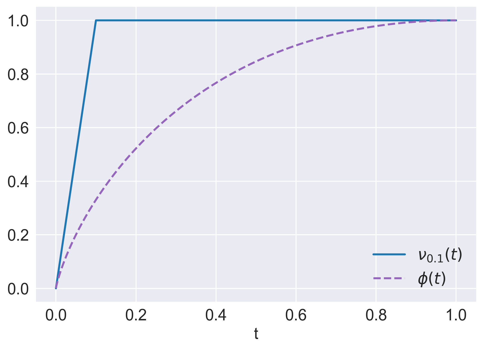
(a) Distortion function

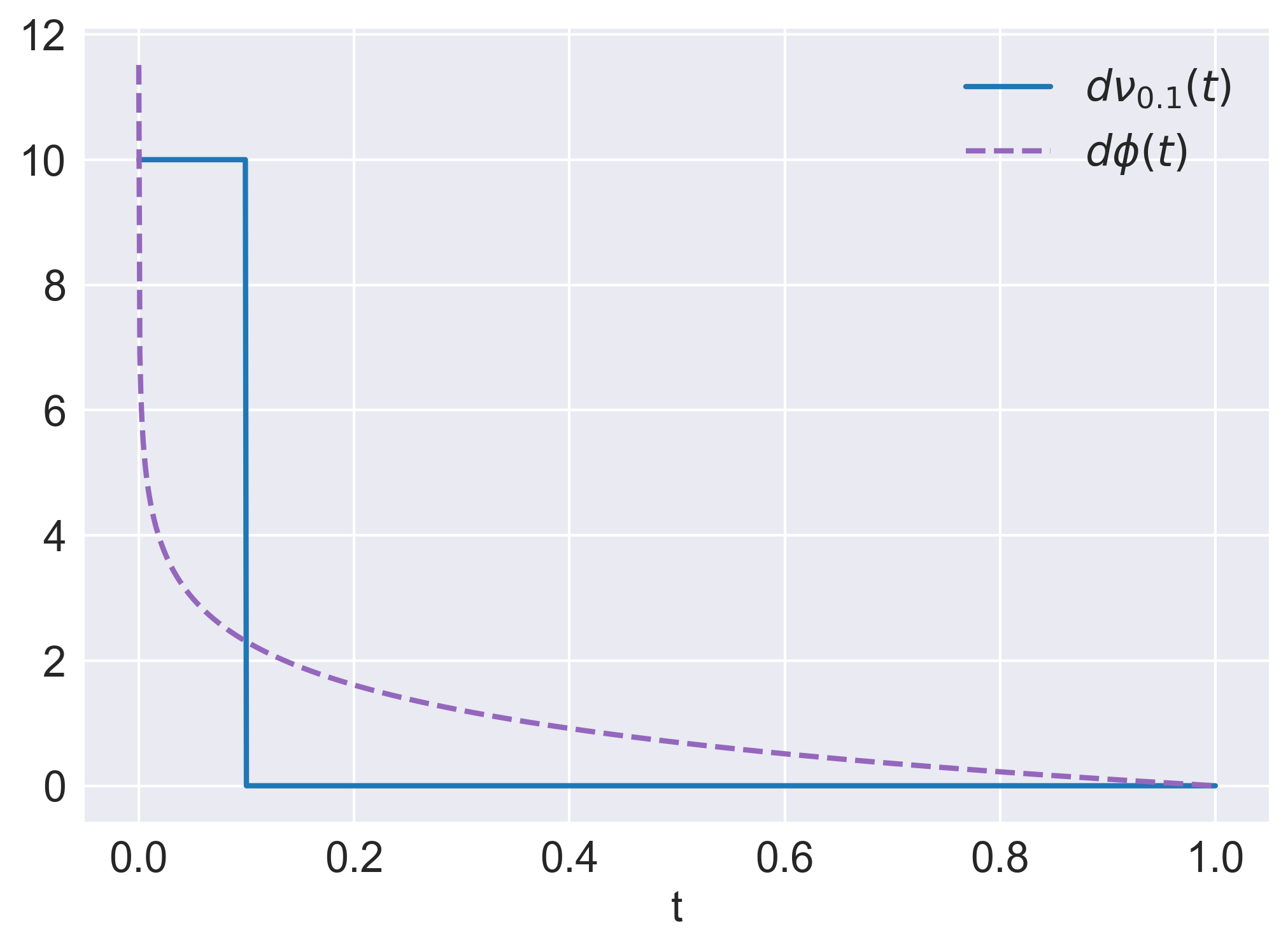
(b) Derivative of distortion function

Figure 6: Distortion functions and their derivatives. $\nu_{0.1}(t)$ and $\phi(t)$ denote the distortion function of $\alpha$-risk at the level $10\%$ and UPR respectively.

S5 Quantile matching between in-sample and out-of-sample for all rolling periods

Figure 7 - 10 present the results of quantile matching of UPR and UPR($\lambda=0.01$). In Figure 7 - 10, we show that the portfolio models based on UPR have the robustness of distribution shift in out-of-sample and regularization mitigates the discrepancy of quantiles between in-sample and out-of-sample.

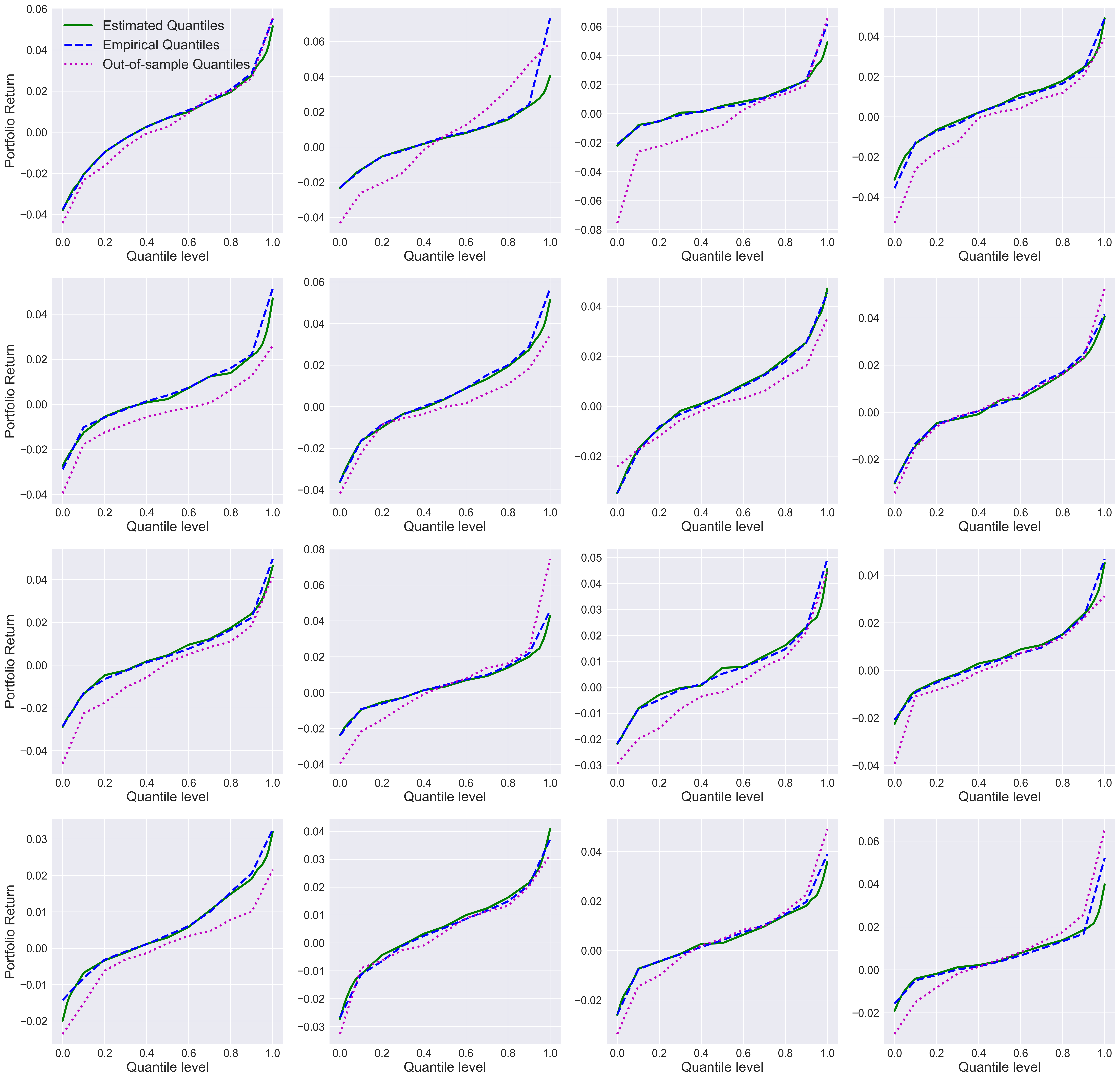
Figure 7: Quantile estimation results of UPR portfolio from evaluation period 1 to 16.

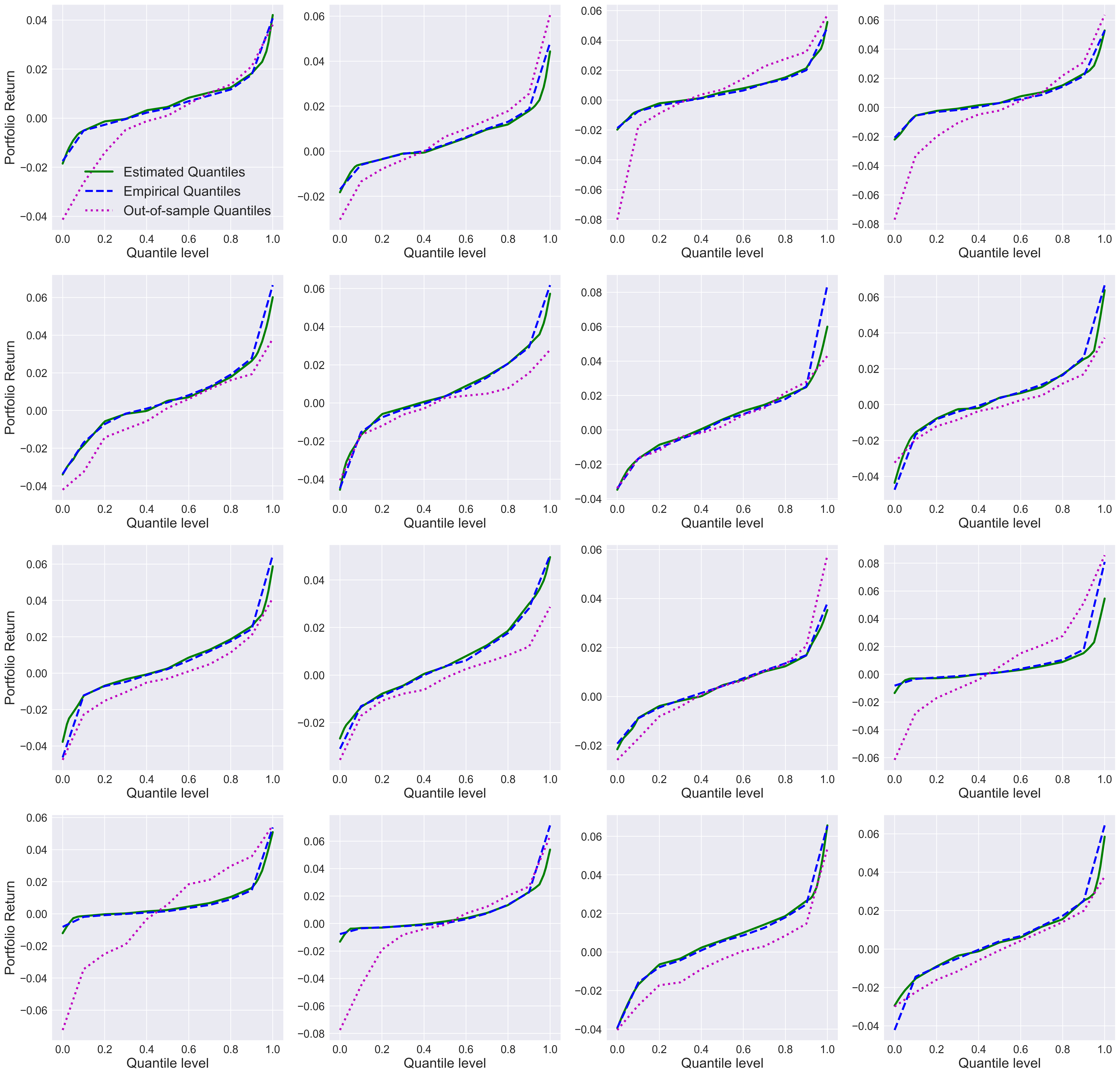
Figure 8: Quantile estimation results of UPR portfolio from evaluation period 17 to 32.

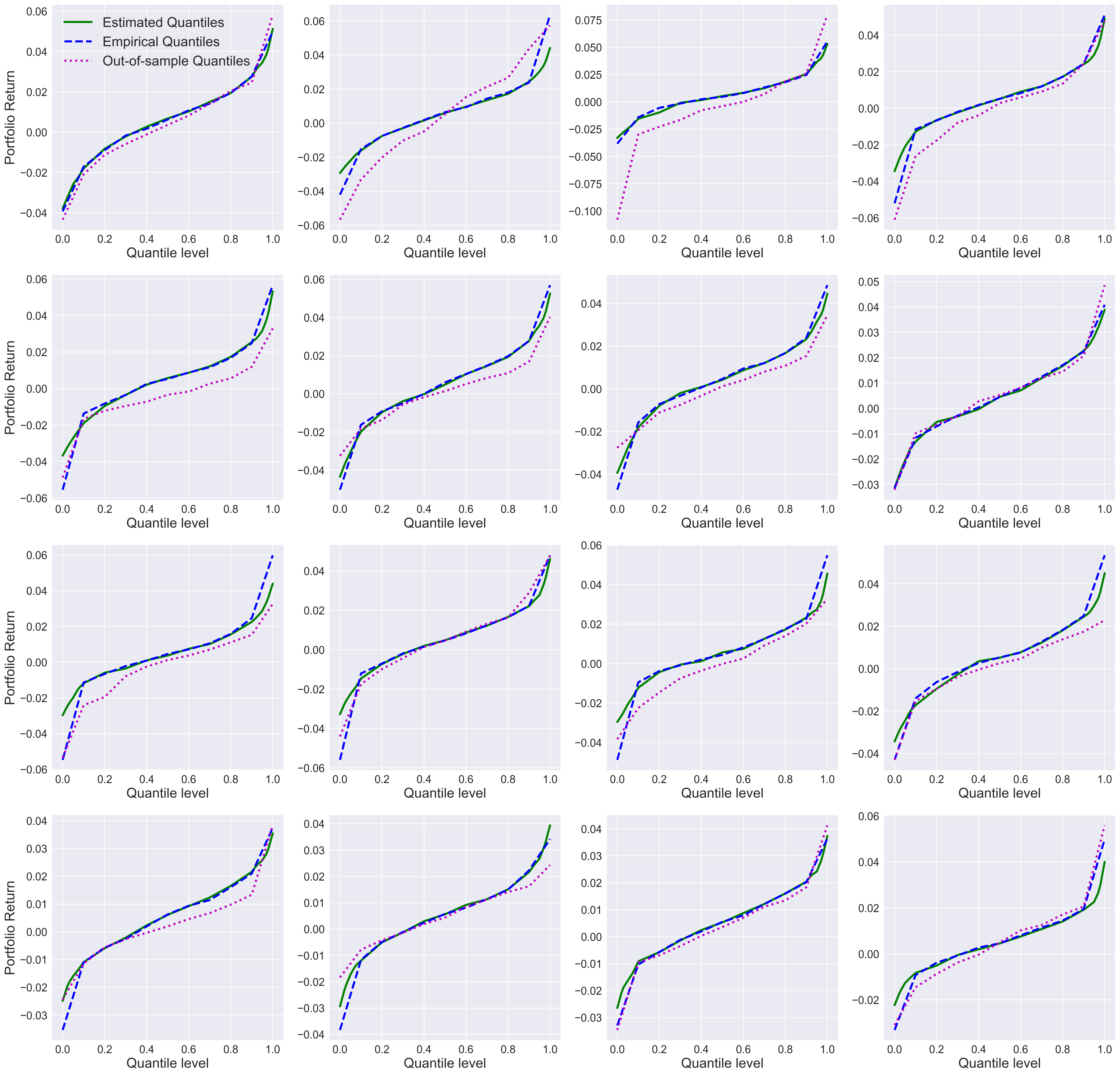
Figure 9: Quantile estimation results of UPR($\lambda=0.01$) portfolio from evaluation period 1 to 16.

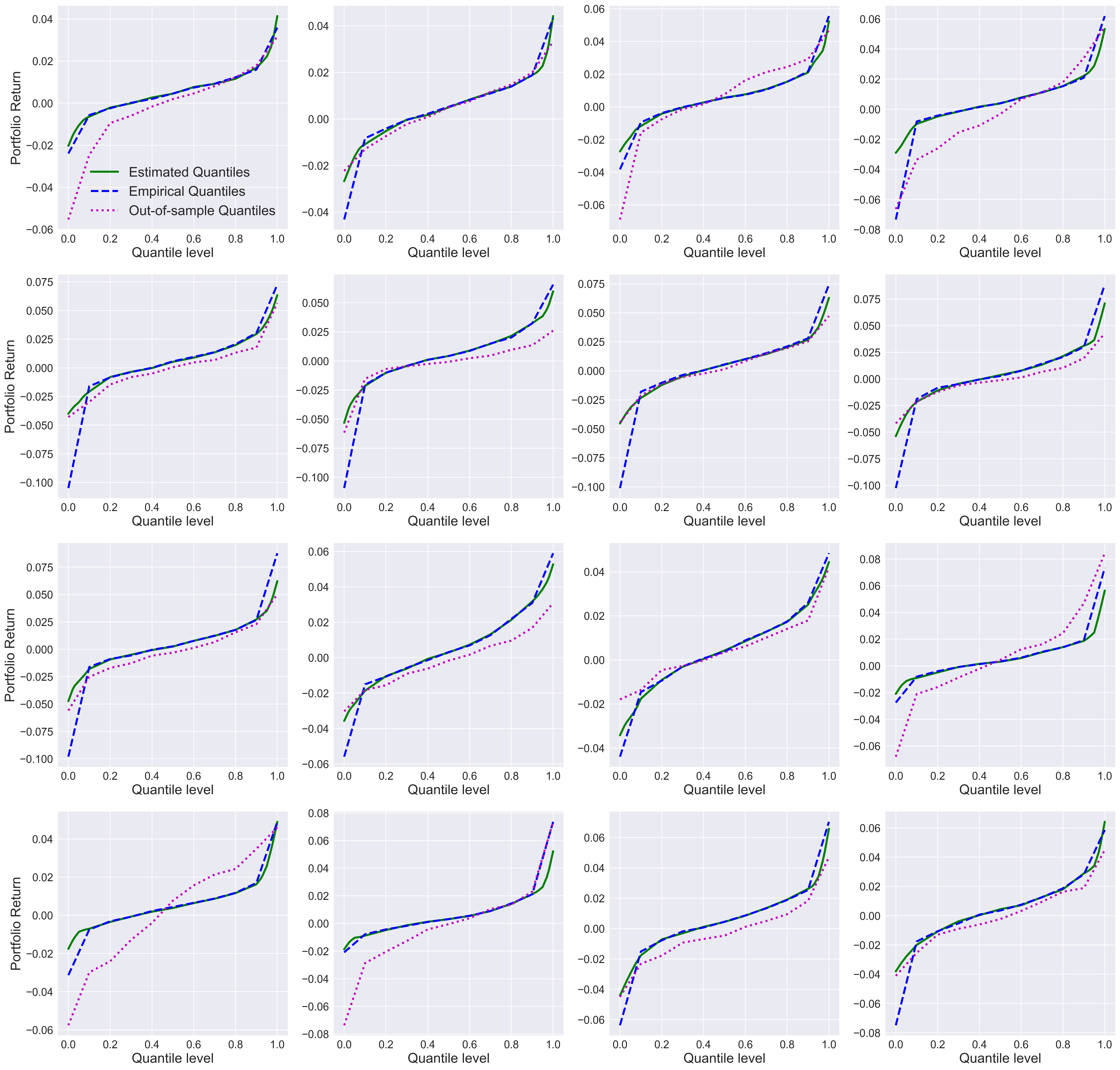
Figure 10: Quantile estimation results of UPR($\lambda=0.01$) portfolio from evaluation period 17 to 32.

References

- Abadi et al., (2015) Abadi, M., Agarwal, A., Barham, P., Brevdo, E., Chen, Z., Citro, C., Corrado, G. S., Davis, A., Dean, J., Devin, M., Ghemawat, S., Goodfellow, I., Harp, A., Irving, G., Isard, M., Jia, Y., Jozefowicz, R., Kaiser, L., Kudlur, M., Levenberg, J., Mané, D., Monga, R., Moore, S., Murray, D., Olah, C., Schuster, M., Shlens, J., Steiner, B., Sutskever, I., Talwar, K., Tucker, P., Vanhoucke, V., Vasudevan, V., Viégas, F., Vinyals, O., Warden, P., Wattenberg, M., Wicke, M., Yu, Y., and Zheng, X. (2015). TensorFlow: Large-scale machine learning on heterogeneous systems. Software available from tensorflow.org.
- Acerbi, (2002) Acerbi, C. (2002). Spectral measures of risk: A coherent representation of subjective risk aversion. Journal of Banking & Finance, 26(7):1505–1518.
- Acerbi and Tasche, (2002) Acerbi, C. and Tasche, D. (2002). Expected shortfall: a natural coherent alternative to value at risk. Economic notes, 31(2):379–388.
- Adam et al., (2008) Adam, A., Houkari, M., and Laurent, J.-P. (2008). Spectral risk measures and portfolio selection. Journal of Banking & Finance, 32(9):1870–1882.
- Artzner et al., (1999) Artzner, P., Delbaen, F., Eber, J.-M., and Heath, D. (1999). Coherent measures of risk. Mathematical finance, 9(3):203–228.
- Bassett Jr et al., (2004) Bassett Jr, G. W., Koenker, R., and Kordas, G. (2004). Pessimistic portfolio allocation and choquet expected utility. Journal of financial econometrics, 2(4):477–492.
- Bertsimas et al., (2004) Bertsimas, D., Lauprete, G. J., and Samarov, A. (2004). Shortfall as a risk measure: properties, optimization and applications. Journal of Economic Dynamics and control, 28(7):1353–1381.
- Bonaccolto, (2019) Bonaccolto, G. (2019). Critical decisions for asset allocation via penalized quantile regression. Mutual Funds.
- Bonaccolto et al., (2018) Bonaccolto, G., Caporin, M., and Paterlini, S. (2018). Asset allocation strategies based on penalized quantile regression. Computational Management Science, 15(1):1–32.
- Bradley and Taqqu, (2003) Bradley, B. O. and Taqqu, M. S. (2003). Financial risk and heavy tails. In Handbook of heavy tailed distributions in finance, pages 35–103. Elsevier.
- Brodie et al., (2009) Brodie, J., Daubechies, I., De Mol, C., Giannone, D., and Loris, I. (2009). Sparse and stable markowitz portfolios. Proceedings of the National Academy of Sciences, 106(30):12267–12272.
- Chen et al., (2019) Chen, J., Dai, G., and Zhang, N. (2019). An application of sparse-group lasso regularization to equity portfolio optimization and sector selection. Annals of Operations Research, pages 1–20.
- Coles et al., (2001) Coles, S., Bawa, J., Trenner, L., and Dorazio, P. (2001). An introduction to statistical modeling of extreme values, volume 208. Springer.
- Das et al., (2014) Das, P., Johnson, N., and Banerjee, A. (2014). Online portfolio selection with group sparsity. In Twenty-Eighth AAAI Conference on Artificial Intelligence.
- (15) DeMiguel, V., Garlappi, L., Nogales, F. J., and Uppal, R. (2009a). A generalized approach to portfolio optimization: Improving performance by constraining portfolio norms. Management science, 55(5):798–812.
- (16) DeMiguel, V., Garlappi, L., and Uppal, R. (2009b). Optimal versus naive diversification: How inefficient is the 1/n portfolio strategy? The review of Financial studies, 22(5):1915–1953.
- Gasthaus et al., (2019) Gasthaus, J., Benidis, K., Wang, Y., Rangapuram, S. S., Salinas, D., Flunkert, V., and Januschowski, T. (2019). Probabilistic forecasting with spline quantile function rnns. In The 22nd International Conference on Artificial Intelligence and Statistics, pages 1901–1910.
- Gneiting and Raftery, (2007) Gneiting, T. and Raftery, A. E. (2007). Strictly proper scoring rules, prediction, and estimation. Journal of the American statistical Association, 102(477):359–378.
- Gneiting and Ranjan, (2011) Gneiting, T. and Ranjan, R. (2011). Comparing density forecasts using threshold-and quantile-weighted scoring rules. Journal of Business & Economic Statistics, 29(3):411–422.
- Jeon et al., (2011) Jeon, J.-J., Kim, Y.-O., and Kim, Y. (2011). Expected probability weighted moment estimator for censored flood data. Advances in water resources, 34(8):933–945.
- Jiang et al., (2016) Jiang, X., Li, J., Xia, T., and Yan, W. (2016). Robust and efficient estimation with weighted composite quantile regression. Physica A: Statistical Mechanics and its Applications, 457:413–423.
- Kingma and Ba, (2015) Kingma, D. P. and Ba, J. (2015). Adam: A method for stochastic optimization. CoRR, abs/1412.6980.
- Kusuoka, (2001) Kusuoka, S. (2001). On law invariant coherent risk measures. In Advances in mathematical economics, pages 83–95. Springer.
- Markowitz, (1952) Markowitz, H. (1952). Portfolio selection. The journal of finance, 7(1):77–91.
- Matheson and Winkler, (1976) Matheson, J. E. and Winkler, R. L. (1976). Scoring rules for continuous probability distributions. Management science, 22(10):1087–1096.
- Nock et al., (2011) Nock, R., Magdalou, B., Briys, E., and Nielsen, F. (2011). On tracking portfolios with certainty equivalents on a generalization of markowitz model: the fool, the wise and the adaptive. In ICML.
- Rahimian and Mehrotra, (2019) Rahimian, H. and Mehrotra, S. (2019). Distributionally robust optimization: A review. arXiv preprint arXiv:1908.05659.
- Rockafellar et al., (2000) Rockafellar, R. T., Uryasev, S., et al. (2000). Optimization of conditional value-at-risk. Journal of risk, 2:21–42.
- Ruszczyński and Shapiro, (2006) Ruszczyński, A. and Shapiro, A. (2006). Optimization of convex risk functions. Mathematics of operations research, 31(3):433–452.
- Shapiro, (2012) Shapiro, A. (2012). Minimax and risk averse multistage stochastic programming. European Journal of Operational Research, 219(3):719–726.
- Shapiro, (2013) Shapiro, A. (2013). On kusuoka representation of law invariant risk measures. Mathematics of Operations Research, 38(1):142–152.
- Sharpe, (1994) Sharpe, W. F. (1994). The sharpe ratio. Journal of portfolio management, 21(1):49–58.
- Taniai and Shiohama, (2012) Taniai, H. and Shiohama, T. (2012). Statistically efficient construction of -risk-minimizing portfolio. Advances in Decision Sciences.
- Van der Vaart, (2000) Van der Vaart, A. W. (2000). Asymptotic statistics, volume 3. Cambridge university press.