Sublinear drag regime at mesoscopic scales in viscoelastic materials

Abstract

Stressed soft materials commonly present viscoelastic signatures in the form of power-law or exponential decay. Understanding the origins of such rheologic behaviors is crucial to find proper technological applications. Using an elastic network model of macromolecules immersed in a viscous fluid, we numerically reproduce those characteristic viscoelastic relaxations and show how the microscopic interactions determine the rheologic response. We find that exponential relaxations are indeed the most common behavior. However, power laws may arise when drag forces between the macromolecules and the fluid are sublinear, which is related to micro-deformations of the macromolecules.

Purely elastic and purely viscous behaviors are limited cases of constitutive equations of materials Lakes2017 . Actual substances may deform and flow, but one of these attributes usually dominates the other, depending on the applied conditions. This solid-liquid duality has teased researchers since at least the 19^th century. Back then, pioneers such as James Maxwell and Ludwig Boltzmann proposed analytical models based on series and parallel associations of springs and dashpots to explain the peculiar characteristics observed in silk, glass fibers, and steel wires Maxwell1867 ; Markovitz1977 . The effective response of such early models invariably presents exponential relaxation decays, regardless of how springs and dashpots are connected. However, these simple approaches are only suited for some viscoelastic materials nowadays.

In modern society, soft matter is ubiquitous and broadly accessible. The emergence of such complex materials has triggered new theoretical models and the improvement of proper experimental techniques to explain and control their viscoelastic properties Sousa2020 ; Sousa2021 . Nanoindentation methods, such as Atomic Force Microscopy, have become essential to characterize viscoelastic features at micro and nanometer scales by probing materials with nano-sized indenters Sousa2017 . The characterization of viscoelastic materials attempts to determine the relaxation function that possesses both qualitative and quantitative information.

Exponential and power-law relaxation functions are the two major types of experimentally probed responses. Polyacrylamide gels Song2017 ; Calvet2004 and aqueous solutions of cationic surfactants Rehage1988 , for instance, present exponential-like responses with a relaxation time for the material to achieve a new equilibrium configuration. On the other hand, living cells Efremov2017 , microgel dispersions Ketz1988 , soft glassy materials Sollich1998 , and hydrogels Larson1999 present a time-invariant power-law-like behavior. As observed in elastic materials Moreira2012 ; Oliveira2014 , macroscopic physical parameters are intrinsically connected to their microscopic interactions and structures Achar2012 ; Yucht2013 ; Milkus2017 .

Power laws and exponentials arise in many physical phenomena having a deep origin in their dynamic processes. For instance, in non-additive entropy systems, many physical variables are described by power-law distributions instead of the traditional exponential functions in the counterpart entropy Tsallis1988 ; Tsallis2009 . Exponential and power-law canonical distributions emerge naturally regarding whether the heat capacity of the heat bath is constant or diverges Murilo2001 . Moreover, power laws are associated with emergence phenomena where exponents display scaling behaviors as they approach criticality Stanley1971 . Systems with precisely the same critical exponents belong to the same universality class, and a small set of universality classes describes almost all material phase transitions.

One of the challenges in material science is linking the physical mechanisms at microscopic scales to macroscopic functional behavior. This approach is especially relevant for soft matter because properties on the molecular scale are linked to conformational and compositional fluctuations on the nanometer and micrometer scale and, in addition, span many orders of magnitude in length Praprotnik2007 ; Qu2011 . Soft matter holds rich structures and various interactions at the mesoscale, where thermal energy per unit volume is negligible, in contrast with the high energy density stored in atomic bonds of crystalline structures Doi2013 . While exponential materials can be modeled by an association of springs and dashpots, such as the so-called standard linear solid model, power-law materials are usually obtained by fractional rheology West2003 ; Jaishankar2012 or glassy rheology models Fabry2001 ; Fabry2003 . However, these models cannot explain the connection between macroscopic responses and their elastic and viscous components.

We design a model of viscoelastic materials composed of an immersed elastic network of macromolecules to study how mesoscopic interactions influence macroscopic rheological behavior in soft materials Araujo2020 . We assume non-linear hydrodynamic drag forces act between the macromolecule and the fluid, where the contribution of elastic and viscous interactions are controlled at the mesoscopic level. By changing the physical parameters of elastic and drag forces, we obtain materials with exponential or power-law relaxations or then an intermediary behavior for responses not clearly characterized. Our results show that exponential behavior is, in fact, the most common regime of deformation, being described by the standard linear solid model. Power-law responses are exceptional outcomes for a particular range of sublinear drag forces.

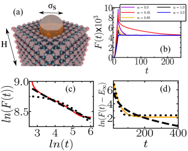
Figure 1: (a) Viscoelastic model made by a face-centered cubic (FCC) lattice of macromolecules immersed in a viscous fluid (not shown in the image). Each spherical particle of diameter $\sigma$ represents a collection of molecules interacting with an effective spring constant $k$ with its twelve closest neighbors. A rigid spherical punch of diameter $\sigma_{s}$ indents the network from top to bottom. $H$ is the number of layers in the vertical direction. (b) Computational force curves for $\gamma=80$ and $k=800$ and several values of $\alpha$ exhibiting different viscoelastic relaxations. The cases for $\alpha=0.45$ and $\alpha=0.85$ are shown in panels (c) and (d), respectively, where the dashed and the dotted lines represent fit with the exponential and power-law model of Eqs. 5 and 6.

Our model consists of $N$ spherical particles of diameter $\sigma$ and mass $m$ arranged in a face-centered cubic (FCC) lattice with dimensions $x\times y\times z$ given by $\sigma H\sin(\pi/3)\times\sigma H\sin(\pi/3)\times\sigma H$, where $H$ is the number of layers in $z$ direction, as shown in Fig. 1(a). Every particle interacts with its twelve nearest neighbors through an elastic potential with an effective spring constant $k$. The spring network is immersed in a viscous fluid, where drag forces act on moving particles. In this coarse-grained approach, the particles represent macromolecules commonly found in suspended polymer chains, colloidal aggregations, and other load-bearing structures of soft matter.

We perform computational indentation assays to probe this network’s effective viscoelastic properties. Firstly, a rigid spherical indenter presses down the network at a constant rate. This loading stage is done during a time $\tau_{l}$ until a maximum indentation depth $\delta_{max}$ is achieved. After that, called dwell stage, the indenter stays still while the network rearranges towards a minimum energy configuration. Particles in the bottom layer are not allowed to move along the $z$-axis (where deformation is applied) but are free to slide horizontally. To avoid finite-size effects, we limit the maximum indentation to less than 10% of the network height Garcia2018 , and thus we apply $\delta_{max}\approx\sigma$.

The equation of motion of the $i_{th}$ particle, at position $\vec{r}_{i}$, is given by the following equation Langevin1908 ; Lemons1997

$$m\frac{d^{2}\vec{r}_{i}}{dt^{2}}=-\nabla U_{i}-\gamma v^{\alpha}_{i}\hat{v}_{i},$$ (1)

where $U_{i}$ is the interaction potential of particle $i$ due to other particles and the indenter, given by

$$U_{i}=\frac{k}{2}\sum_{j}(r_{ij}-\ell)^{2}+\epsilon\left[\frac{\sigma}{r_{is}-(\sigma_{s}-\sigma)/2}\right]^{\xi}.$$ (2)

The summation in the first part runs over the neighbors, where $r_{ij}=|\vec{r}_{i}-\vec{r}_{j}|$ and $\ell$ are, respectively, the distance and the equilibrium distance between the centers of particles $i$ and $j$. The last term in Eq. (2) represents a hard-core potential applied only to those particles in contact with the indenter, where $\epsilon$ is an energy parameter, and $r_{is}=|\vec{r}_{i}-\vec{r}_{s}|$ is the distance between the center of the particle and the indenter. The exponent $\xi$ must be large enough to keep the stiffness of the indenter.

The last term of Eq. (1) represents a generalized drag force acting oppositely to the particle velocity, $\vec{v}_{i}=v_{i}\hat{v}_{i}$, with magnitude given by $\gamma v^{\alpha}_{i}$, where $\gamma$ and $\alpha$ are related to the particle geometry and the fluid properties in which the particles are immersed. Dissipation vanishes for $\gamma=0$, leading to purely elastic networks where our model reproduces the well-known Hertz behavior for mechanical contacts Araujo2020 . However, when local friction becomes relevant, $\gamma>0$, the model may produce distinguished behaviors of viscoelastic materials. Notice that $\alpha=1$ and $\alpha=2$ represent typical values for drag forces acting on rigid structures. The linear regime, known as Stoke’s law, arises for small Reynolds numbers when viscous forces dominate over inertial forces, where $\gamma$ is proportional to the medium’s viscosity and the particle’s diameter. On the other hand, the quadratic drag is dominant for large Reynolds numbers. In this case, $\gamma$ is proportional to the medium’s density and the cross-sectional area of the particle.

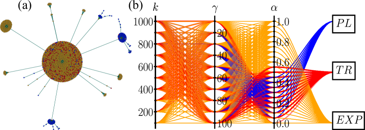
Figure 2: (a) Graph visualization of the clustering process using K-means method. Each dot represents a computational experiment for a given combination of $k$, $\gamma$, and $\alpha$, and the colors represent different relaxation outcomes, namely, power-law (PL) in blue, exponential (EXP) in yellow and transitional behavior (TR) in red. (b) Parallel plot showing how different values of the mesoscopic network parameters lead to different types of viscoelastic relaxation. Each line crosses a combination of $k$, $\gamma$, $\alpha$, and the corresponding rheological behavior.

The physical origins of the sublinear regime ($\alpha<1$), however, are entirely different and are related to the deformability/adaptability of bodies subjected to drag forces Vogel1994 . Many living beings present sublinear drag behaviors, where deformability is a survival strategy to protect their fragile structures under hydrodynamic conditions. Characterizing the drag exponents in deformable systems is recurrent in botany, aerodynamics, and hydrodynamics Vogel1989 ; Favier2009 ; Gosselin2010 ; John2015 . Typical drag exponents for algae are as small as 0.34 Vogel1984 . On the other hand, tulip and willow oak trees are more rigid and present exponents close to unity, $\alpha=0.92$ and $\alpha=0.94$ Vogel1989 , respectively. The limiting case of $\alpha=0$ corresponds to constant frictional forces, regardless of the particle velocity. In our model, micro deformations are associated with a new molecular arrangement of the macromolecules.

The numerical solution of Eq. (1) is performed through molecular dynamics simulations Rapaport2004 ; Araujo2017 with periodic boundary conditions applied to the horizontal plane, and time integration is done with the velocity Verlet algorithm with time step $dt$. See Param for the parameters used. The force is computed as the sum of all collisions on the indenter at each time step. Each set of $k$, $\gamma$, and $\alpha$ represents a specific material and defines the macroscopic viscoelastic responses. To investigate how microscopic properties lead to the rheological behavior of the entire network, we perform simulations varying the spring constant between 100 and 1000, the drag constant between 10 and 100, and the drag exponent between 0.0 and 1.0, totalizing 2100 different networks.

Figure 1(b) shows typical force curves for $\gamma=80$ and $k=800$ and different values of the drag exponent. $F(t)$ is the computational analogous of an indentation assay used to characterize macroscopic responses of actual materials. In the loading stage, the indenter slowly deforms the network until the contact force reaches its maximum value, which is inversely proportional to $\alpha$. In the dwell stage, when the indenter stays still, $F(t)$ relaxes until part of the mechanical energy is lost through friction. The timescale of such dissipation depends on $\alpha$ in a highly complex fashion. For $\alpha=2$, dissipation is fast enough so that the response behavior is qualitatively identical to a perfectly elastic network. For $\alpha<1$, drag forces slowly remove energy from the network leading to a viscoelastic decay.

In a continuum approach, the analytical time-dependent contact force of a viscoelastic sample indented by a spherical punch follows the convolution integral Araujo2020

$$\mathcal{F}(t)=\int_{0}^{t}R(t-t^{{}^{\prime}})\frac{d\delta^{\frac{3}{2}}(t^{{}^{\prime}})}{dt^{{}^{\prime}}}dt^{{}^{\prime}},$$ (3)

where $R(t)$ is the relaxation function and $\delta(t)$ the indentation depth history. The contact force in Eq. (3) is normalized by the constant $4\sqrt{\sigma_{s}}\delta_{max}^{\frac{3}{2}}/3(1-\nu^{2})$, where $\nu$ is the Poisson coefficient. Typical relaxation behaviors for viscoelastic materials are given by

$$R_{P}(t) = E_{\infty}+\Delta E\,\,t^{-\beta},$$

$$R_{E}(t) = E_{\infty}+\Delta E\,\,e^{-\frac{t}{\tau}},$$ (4)

where $R_{P}(t)$ is the relaxation model for power-law materials with an exponent $\beta$ and $R_{E}(t)$ for exponential materials with relaxation time $\tau$. In both models, $E_{\infty}$ is the elastic modulus at considerable times when the material is completely relaxed, and $\Delta E$ is the difference between the maximum value, at $t=\tau_{l}$, and $E_{\infty}$. We assume that materials become perfectly elastic after some time, although this long-time elasticity plateau is only sometimes observed in actual materials Footnote . However, micro-deformations are allowed only due to the movement of the pseudo-atoms, which is represented by the sublinear drag regime. Solving Eq. (3) with Eqs. (4) in the dwell stage leads, respectively, to

$$\mathcal{F}_{P}(t) = E_{\infty}+a\,t^{-\beta},$$ (5)

$$\mathcal{F}_{E}(t) = E_{\infty}+b\,e^{-\frac{(t-\tau_{l})}{\tau}}-c\,e^{-\frac{t}{\tau}},$$ (6)

where the constant $a\approx\frac{\Delta E}{\Gamma(1-\beta)}$ is obtained by expanding the incomplete beta function, $\Gamma(1-\beta)$ is the gamma function, and $b=\frac{3\tau}{2\tau_{l}}\Delta E$ and $c=\frac{3\sqrt{\pi}}{4}(\frac{\tau}{\tau_{l}})^{\frac{3}{2}}\Delta E\,\mathrm{erfi}(\sqrt{\frac{\tau_{l}}{\tau}})$, where erfi($\sqrt{\frac{\tau_{l}}{\tau}}$) is the imaginary error function of $x$.

Fitting the dwell part of the force curve allows us to map the macroscopic mechanical properties ($E_{\infty}$, $\Delta E$, $\tau$, $\beta$) with the mesoscopic parameters ($k$, $\gamma$ and $\alpha$) as done previously for $\alpha=1$ Araujo2020 . Here we focus on finding the qualitative rheological behavior rather than describing relations among parameters. Figures 1(c) and (d) show the same force curves as in (b) for $\alpha=0.45$ and $\alpha=0.85$, respectively, where the curves are fitted both with $\mathcal{F}_{P}(t)$ and $\mathcal{F}_{E}(t)$. Clearly, the $\alpha=0.45$ case is better fitted with the power-law model, while $\alpha=0.85$ with an exponential.

The mean-square error determines the goodness-of-fit parameter between the obtained numerical force curve $F(t)$ and the analytical force models given in Eqs. 5 and 6,

$$\chi_{M}=\frac{1}{N_{p}}\sum_{i=1}^{N_{p}}\left[F(t_{i})-\mathcal{F}_{M}(t_{i})\right]^{2},$$ (7)

where $N_{p}$ is the number of points in the force curves and $M$ stands for exponential ($E$) or power-law ($P$) model type. This statistical index, calculated for each combination of $k$, $\gamma$, $\alpha$, is used in a K-means method as an unsupervised clustering strategy Geron2019 ; Sinaga2020 to classify the computational force curves as either an exponential or a power-law behavior, or even a transitional regime that cannot be clearly classified. In this machine learning process, the classification of the material takes into account not only the values of $\chi_{E}$ and $\chi_{P}$ but also the trends and distributions in the phase space of $\chi_{E}$ and $\chi_{P}$. Figure 2(a) shows the graph visualization of this clustering process. The exponential behavior is indeed the most common one, as shown in the big cluster in Fig. 2(a), but small groups of power-law materials are also observed. The parallel coordinates plot in Fig. 2(b) summarizes the rheological outcomes. Each line passes through every combination of $k$, $\gamma$, and $\alpha$ ending up in one of the three boxes representing the response behavior of the network.

To understand why small clusters of power-law materials form in Fig. 2(a), we must investigate the impact of considering sublinear drag regimes. Fig. 3 shows the normalized probability $P(\alpha)$ of finding PL, EXP, or TR behavior for a given $\alpha$. In panel (a), $P(\alpha)$ is computed for all values of $k$ and $\gamma$ considered here. The three distributions strongly overlap, making classification a challenging exercise. In panel (b), on the other hand, we remove small values of $k$ and $\gamma$. For networks not too soft, $k\geq 800$, and not too elastic, $\gamma\geq 80$, those distributions split for different regions of $\alpha$, and the drag exponent becomes the central controller to characterize the macroscopic behavior. Exponential behaviors are found mainly for $\alpha\lessapprox 0.2$ and $\alpha\gtrapprox 0.55$, while the relaxation is a power law for $\alpha$ between 0.3 and 0.45. For intersecting values of $\alpha$, the superposition of the probabilities of PL and EXP leaves doubt in classifying the material either as an exponential or a power law.

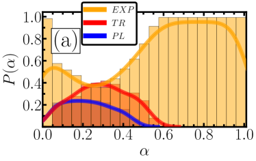
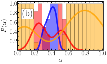
Figure 3: The probability that a given $\alpha$ leads to a power law (blue bars), an exponential (yellow bars), or a transitional response (red bars). The solid lines show the probability density computed by the KDE (kernel density estimation) algorithm. Panel (a) shows results for the whole range of $k$ and $\gamma$, while panel (b) considers only networks with $k$ ($k\geq 800$) and $\gamma$ ($\gamma\geq 80$).

For those cases where the network presents a power-law behavior, we show in Fig. 4 the relationship between the macroscopic relaxation exponent $\beta$ and the drag exponent. For each value of $\alpha$, there is a small dispersion distribution of $\beta$ whose mean range is between 1.05 and 1.35. Actual materials exhibiting power-law relaxation usually present smaller exponents and exhibit structural disorder and metastability Sollich1997 ; Fabry2001 ; Fabry2003 ; Jaishankar2012 . Computational investigations of disordered two-dimensional networks obtained relaxation exponents between 0.5 and 0.75, depending on the network arrangement Milkus2017 . Our simulations exhibit macroscopic relaxation exponents above 1.0, mainly because our viscoelastic solid model is structurally ordered and stable, restricting the viscoelastic responses to faster relaxation regimes. Our results clearly show that structural disorder is not a mandatory ingredient for power-law-like viscoelasticity and can only change the exponent.

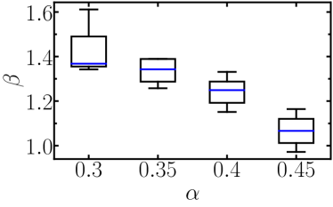
Figure 4: For those networks classified as a power-law material in Figure 2(b), we show the relationship between the relaxation exponent $\beta$ and the mesoscopic drag exponent $\gamma$.

In conclusion, we show why viscoelastic materials present power-law or exponential relaxation responses. Using molecular dynamics simulations, we perform numerical indentations onto a network of interacting macromolecules immersed in a fluid and reproduce typical viscoelastic signatures as those found experimentally. The macromolecules interact with the fluid through a non-linear drag regime given by $\gamma v^{\alpha}$, where $\gamma$ and $\alpha$ are mesoscopic parameters, and $v$ is the particle’s velocity. For each set of the interacting parameters, we classify the macroscopic viscoelasticity using an unsupervised clustering algorithm according to the type of relaxation of the deformed network, namely, exponential or power-law relaxations or transitional behavior between them. While exponential behaviors are predominant, power laws may arise in the sublinear regime. In fact, the drag exponent alone may explain the macroscopic viscoelastic relaxation for materials not too elastic nor too soft. More specifically, power-law responses are found for $0.3\lessapprox\alpha\lessapprox 0.45$, while exponential responses for $0.0\lessapprox\alpha\lessapprox 0.2$ and $0.55\lessapprox\alpha\lessapprox 1.0$.

- (1) R. S. Lakes, Viscoelastic Solids (CRC Press, 2017).
- (2) J. C. Maxwell, On the dynamical theory of gases, Phil. Trans. Royal Soc. London 157, 49 (1867).
- (3) H. Markovitz, Boltzmann and the beginning of linear viscoelasticity, Trans. Soc. Rheology 21, 381 (1977).
- (4) J. S. de Sousa, R. S. Freire, F. D. Sousa, M. Radmacher, A. F. B. Silva, M. V. Ramos, A. C. O. Monteiro-Moreira, F. P.Mesquita, M. E. A. Moraes, R. C. Montenegro, and C. L. N. Oliveira, Double power-law viscoelastic relaxation of livingcells encodes motility trends, Sci. Rep. 10, 4749 (2020).
- (5) F. B. de Sousa, P. K. V. Babu, M. Radmacher, C. L. N. Oliveira, and J S de Sousa Multiple power-law viscoelastic relaxation in time and frequency domains with atomic force microscopy, J. Phys. D: Appl. Phys. 54, 335401 (2021).
- (6) J. S. de Sousa, J. A. C. Santos, E. B. Barros, L. M. R. Alencar, W. T. Cruz, M. V. Ramos, and J. Mendes Filho, Analytical model of atomic-force-microscopy force curves in viscoelastic materials exhibiting power law relaxation, App. Phys. Rev. 1, 8 (2017).
- (7) R. Song, G. Jiang, and K. Wang, Gelation mechanism and rheological properties of polyacrylamide crosslinking with polyethyleneimine and its plugging performance in air-foam displacement, App. Polymer Sci. 4 11 (2017).
- (8) D. Calvet, J. Y. Wong, and S. Giasson, Rheological Monitoring of Polyacrylamide Gelation: Importance of Cross-Link Density and Temperature, Macromolecules 7769 7771 (2004).
- (9) H. Rehage and H. Hoffmann, Rheological properties of viscoelastic surfactant systems, The Journal of Physical Chemistry 4713 4719 (1988).
- (10) Y. M. Efremov, W.-H. Wang, S. D. Hardy, R. L. Geahlen and A. Raman, Measuring nanoscale viscoelastic parameters of cells directly from AFM force-displacement curves, Nature 4 11 (2017).
- (11) R. J. Ketz, Jr., R. K. Prud’homme and W. W. Graessley, Rheology of concentrated microgel solutions, Rheologica Acta 535 531 (1988).
- (12) P. Sollich, Rheological constitutive equation for a model of soft glassy materials, Phys. Rev. E 58 738 (1998).
- (13) R. G. Larson, The Structure and Rheology of Complex Fluids (Oxford University Press, 1999).
- (14) A. A. Moreira, C. L. N. Oliveira, A. Hansen, N. A. M. Araújo, H. J. Herrmann, and J. S. Andrade, Fracturing Highly Disordered Materials, Phys. Rev. Lett. 109, 255701 (2012).
- (15) C. L. N. Oliveira, J. H. T. Bates, and B. Suki, A network model of correlated growth of tissue stiffening in pulmonary fibrosis, New J. Phys. 16, 065022 (2014).
- (16) B. N. Achar, and J. W. Hanneken, ”Microscopic Formulation of Fractional Theory of Viscoelasticity”, in Viscoelasticity - From Theory to Biological Applications. London, United Kingdom: IntechOpen, 2012.
- (17) M. G. Yucht, M. Sheinmanb and C. P. Broedersz, Dynamical behavior of disordered spring networks, Soft Matter 9, 7000 (2013).
- (18) R. Milkus, and A. Zaccone, Atomic-scale origin of dynamic viscoelastic response and creep in disordered solids, Phys. Rev. E 95, 023001 (2017).
- (19) C. Tsallis, Possible Generalization of Boltzmann-Gibbs Statistics, J. Stat. Phys. 52, 479 (1998).
- (20) C. Tsallis, Nonadditive entropy and nonextensive statistical mechanics - an overview after 20 years, Braz. J. Phys. 39, (2a) (2009).
- (21) M. P. Almeida, Generalized entropies from first principles, Phys. A 300, 424 (2001).
- (22) H. E. Stanley, Introduction to Phase Transitions and Critical Phenomena (Oxford, 1971).
- (23) M. Praprotnik, L. D. Site and K. Kremer, Multiscale Simulation of Soft Matter: From Scale Bridging to Adaptive Resolution, Rev. Phys. Chem. 547, 571 (2007).
- (24) Z. Qu, A. Garfinkel, J. N. Weiss, M. Nivala, Multi-scale modeling in biology: How to bridge the gaps between scales?, ELSEVIER 21, 31 (2011).
- (25) M. Doi, Soft Matter Physics (Oxford, 2013).
- (26) B. J. West, M. Bologna, and P. Grigolini, Physics of Fractal Operators (Springer, 2003).
- (27) A. Jaishankar and G. H. McKinley, Power-law rheology in the bulk and at the interface: quasi-properties and fractional constitutive equations, Proc. R. Soc. A 469, 20120284 (2012).
- (28) B. Fabry, G. N. Maksym, J. P. Butler, M. Glogauer, D. Navajas, and J. J. Fredberg, Scaling the microrheology of living cells, Phys. Rev. Lett. 87, 148102 (2001).
- (29) B. Fabry, G. N. Maksym, J. P. Butler, M. Glogauer, D. Navajas, N. A. Taback, E. J. Millet, and J. J. Fredberg, Time scale and other invariants of integrative mechanical behavior in living cells, Phys. Rev. E 68, 041914 (2003).
- (30) J. L. B. de Araújo, J. S. de Sousa, W. P. Ferreira, and C. L. N. Oliveira, Viscoelastic multiscaling in immersed networks, Phys. Rev. Research 2, 033222 (2020).
- (31) P. D. Garcia and R. Garcia, Determination of the Elastic Moduli of a Single Cell Cultured on a Rigid Support by Force Microscopy, Biophys. J. 114, 2923 (2018).
- (32) P. Langevin, Sur la théorie du mouvement brownien, C. R. Acad. Sci. (Paris) 146, 530 (1908).
- (33) D. S. Lemons and A. Gythiel, Paul Langevin’s 1908 paper “On the Theory of Brownian Motion” [“Sur la théorie du mouvement brownien,” C. R. Acad. Sci. (Paris) 146, 530 (1908)], Am. J. Phys. 1081, 1081 (1997).
- (34) S. Vogel, Life in moving fluids: the philosophical biology of flow (Princeton University Press. 1994).
- (35) F. Gosselin, E. de Langre and B. A. Machado-Almeida, Drag reduction of flexible plates by reconfiguration, J. Fluid Mech. 650, 319 (2010).
- (36) S. Vogel, Drag and Reconfiguration of Broad Leaves in High Winds, Journal of Experimental Botany 945, 948 (1989).
- (37) J. A. Chapman, B. N. Wilson, and J. S. Gulliver, Drag force parameters of rigid and flexible vegetal elements, Water Resources Research 3293, 3292-3302 (2015).
- (38) J. Favier, A. Dauptain, D. Basso and A. Bottaro, Passive separation control using a self-adaptivehairy coating, J. Fluid Mech. 627, 451 (2009).
- (39) S. Vogel, Drag and Flexibility in Sessile Organisms 1, Amer. Zoll. 40, 44 (1984).
- (40) D. C. Rapaport, The Art of Molecular Dynamics Simulation - second edition (Cambridge University Press, 2004)
- (41) J. L. B. de Araújo, F. F. Munarin, G. A. Farias, F. M. Peeters, and W. P. Ferreira, Structure and reentrant percolation in an inverse patchy colloidal system, Phys. Rev. E 95, 062606 (2017).
- (42) The dimensionless length, mass, and energy units are given, respectively, by , , , and the timestep , where the time unit has the following relation . Other length parameters are given by , , and , and some exponents by and . The number of particles in the network is .
- (43) This assumption is necessary to avoid high-pressure effects in our numerical model. For instance, if the external force is large enough to ultimately compress the small particles until a condensate network is formed, any additional pressure would induce the deformation of those particles.
- (44) A. Geron, Hands-On Machine Learning with Scikit-Learn, Keras, and TensorFlow, Published by O’Reilly Media, Inc., 1005 Gravenstein Highway North, Sebastopol, CA 95472., 1150 (2019).
- (45) K. P. Sinaga and M. Yang, Unsupervised K-Means Clustering Algorithm, IEEE Access 8, 80716 (2020).
- (46) P. Sollich, F. Lequeux, P. Hébraud, M. E. Cates, Rheology of Soft Glassy Materials, Phys. Rev. Lett. 78, 2020 (1997).