Design, Control, and Motion Strategy of TRADY: Tilted-Rotor-Equipped Aerial Robot With Autonomous In-flight Assembly and Disassembly Ability

Abstract

Various types of aerial robots have been demonstrated in prior works with the intention of enhancing their maneuverability or manipulation capabilities. However, the problem remains in earlier researches that it is difficult to achieve both mobility and manipulation capability. This issue arises due to the fact that aerial robots with high mobility possess insufficient rotors to execute manipulation tasks, while aerial robots with manipulation ability are too large to achieve high mobility. To tackle this problem, we introduce in this article a novel aerial robot unit named TRADY. TRADY is a tilted-rotor-equipped aerial robot with autonomous in-flight assembly and disassembly capability. It can be autonomously combined and separated from another TRADY unit in the air, which alters the degree of control freedom of the aircraft by switching the control model between the under-actuated and fully-actuated models. To implement this system, we begin by introducing a novel design of the docking mechanism and an optimized rotor configuration. Additionally, we present the configuration of the control system, which enables the switching of controllers between under-actuated and fully-actuated modes in the air. We also include the state transition method, which compensates for discrete changes during the system switchover process. Furthermore, we introduce a new motion strategy for assembly/disassembly motion that incorporates recovery behavior from hazardous conditions. Finally, we evaluate the performance of our proposed platform through experiments, which demonstrated that TRADY is capable of successfully executing aerial assembly/disassembly motions with a rate of approximately 90%. Furthermore, we confirmed that in the assembly state, TRADY can utilize full-pose tracking, and it can generate more than nine times the torque of a single unit. To the best of our knowledge, this work represents the first time that a robot system has been developed that can perform both assembly and disassembly while seamlessly transitioning between fully-actuated and under-actuated models.

I Introduction

In recent years, aerial robots have undergone significant development [1], [2] and have proven to be useful for various practical applications. Compact aerial robots such as quadrotors with terrain-independent mobility have enabled

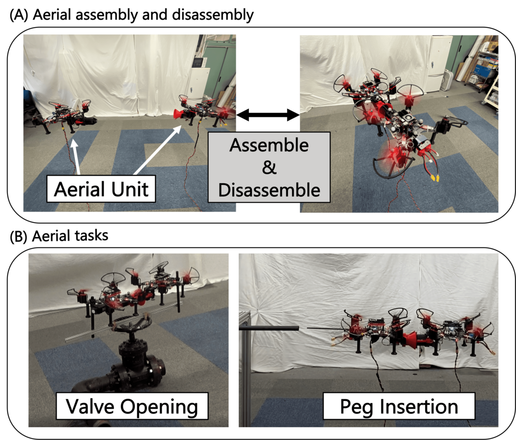
Figure 1: The proposed robot platform TRADY: Tilted-Rotor-Equipped Aerial Robot With Autonomous In-flight Assembly and Disassembly AbilitY. (A)The unitary state and the assembly state of TRADY. (B)Task execution capability of TRADY.

various autonomous applications such as cinematography [3], inspection [4], disaster response [5], and surveillance [6]. Furthermore, to enhance mobility, numerous designs that enable robots to navigate through narrow spaces have been proposed, such as quadrotors with morphing capabilities that allow their airframe to shrink [7, 8, 9, 10, 11]. On the other hand, there has been a growing demand for aerial robots to possess manipulation capabilities, which require larger controllable degrees of freedom (DoF) and available force and torque (wrench). As a solution, more intricate and sizable aerial robots have been developed, including multirotors equipped with over six tiltable rotors enabling omni-directional control [12], and arm-manipulator-installed multirotors capable of interacting with the environment [13, 14, 15].

However, a significant issue in the conventional works is the inherent trade-off between mobility and manipulation capability. To clarify, High-mobility under-actuated aerial robots often lack the necessary controllable DoF and available wrench to achieve manipulation tasks, whereas fully-actuated robots with manipulation capability often lack compactness. To address this problem, some researchers have proposed a transformable multilink design [16, 17, 18] that enables robots to navigate narrow spaces and perform manipulation tasks using their entire body [19]. Nonetheless, these transformable aerial robots require a significant number of additional actuators, making them heavy, and even with transforming capability, it remains challenging to achieve the same maneuverability as a small quadrotor in a narrow space with three-dimensional complexity.

In this article, we present a solution to the aforementioned trade-off problem by introducing TRADY, a novel aerial robot platform that can perform aerial assembly and disassembly motion, as depicted in Fig. 1 (A), while changing its controllable DoF and available wrench. In its unitary state, TRADY is a compact under-actuated quadrotor, however, in its assembly state, it becomes a fully-actuated octorotor, enabling it to execute aerial manipulation tasks as depicted in Fig. 1 (B).

I-A Related works

TRADY is a type of modular aerial robot, and previous studies have developed several other modular aerial robots. In [20], Naldi et al. introduce a single ducted-fan module, and in [21], a tetrahedron-shaped quadrotor module consisting of four fractal single-rotor submodules is presented. Furthermore, in [22], a modular quadrotor equipped with tilted rotors is proposed. These modular aerial robots can combine with one another and expand their degrees of freedom and wrench, however, [20, 21, 22] are currently not focused on self-assembly/disassembly. On the other hand, several aerial robots capable of self-assembly or self-disassembly have previously been developed. For instance, in [23], [24], a robot unit composed of wheels and rotors capable of docking on the ground and taking off afterwards is presented. Additionally, in [25], a modular quadrotor with the capability of aerial self-assembly is proposed, followed by one with the ability of aerial self-disassembly proposed in [26]. However, the issue that remains is that the robot presented in [23], [24] is restricted to assembly/disassembly on the ground, and mid-air assembly/disassembly are unfeasible, whereas [25], [26] virtually specialize in either aerial assembly or aerial disassembly but not both. Futhermore, assembly or disassembly motion demonstrated in [23, 24, 25, 26] are unaccompanied by the alternation of controllable DoF, implying that the robots are under the control of an under-actuated model in both the assembly and unitary states. The utilization instance of TRADY envisioned in this research comprises tasks illustrated in Fig. 2. To accomplish this, movement in a narrow space must be carried out in the unitary state, and during manipulation tasks, the units must assemble to extend the controllable DoF and wrench, then return to the unitary state afterwards. Therefore, the compatibility of aerial self-assembly and self-disassembly, and the consequent alteration of the controllable DoF, remain crucial unachieved issues that are necessary for realizing TRADY. In this study, we tackle this issue from the perspectives of design, control, and motion strategy.

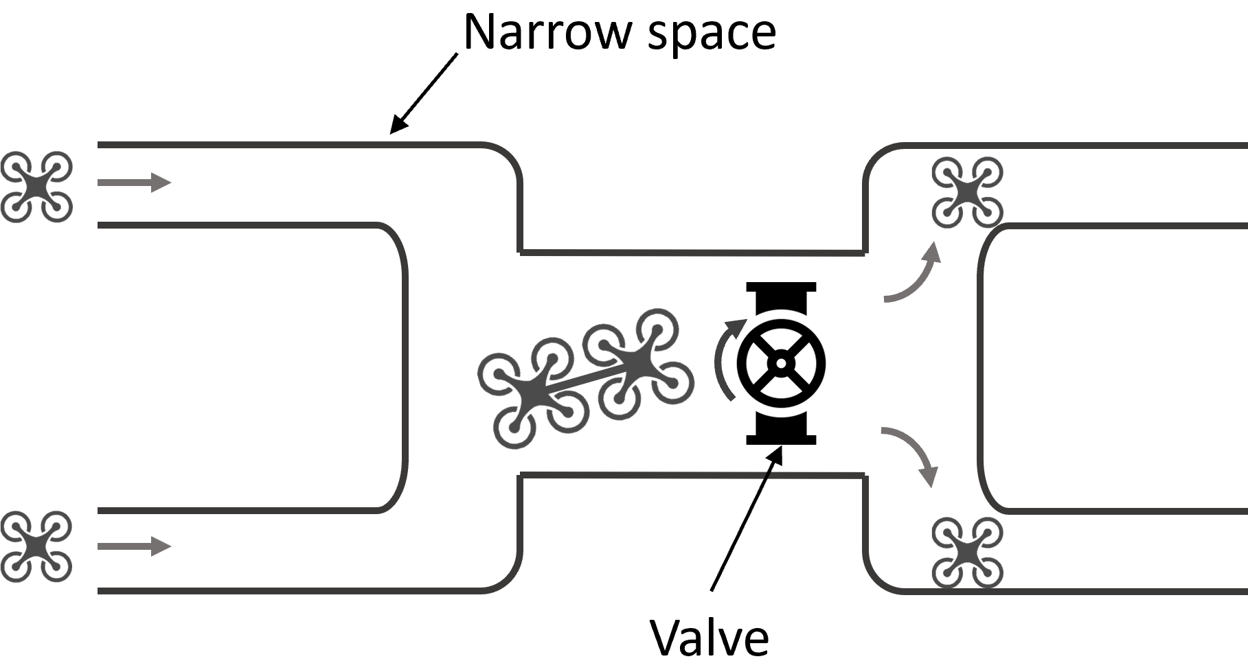
Figure 2: Application example that can be realized with TRADY developed in this work: Valve opening and closing tasks in narrow and complex spaces.

Concerning the design of the self-docking mechanism, various designs have been previously presented. For example, in [27], autonomous boats equipped with hook-string docking mechanisms are introduced. In this system, the hooks of the male mechanism attach to the loop of string on the female mechanism, and the female side winches the loop of thread and the male mechanism together, thereby merging the modules. While this mechanism works effectively on the water, the coupling force is not sufficiently strong to be applicable to aerial systems. On the other hand, in [25], to achieve aerial docking, a quadrotor is enclosed in a rectangular frame equipped with permanent magnets. While this mechanism can construct a highly rigid structure, it has the disadvantage of being unable to release the coupling once it has been established. On the contrary, a quadrotor unit that can undock through the torque generated by the unit itself is developed in [26]. However, to achieve undocking capability, the docking mechanism is significantly downsized in comparison to the one used in [25], and the design is not suitable for aerial docking. Furthermore, as the docking can be released through the torque output of a unit, the strength of the mechanism becomes a bottleneck for available torque, making it arduous to execute tasks that necessitate high torque. As an alternative method for releasing the magnetic coupling, the utilization of elastic energy is proposed in [28]. The mechanism proposed in [28] shortens the internal spring of the mechanism using an actuator, and releases it to generate restoring force, thereby releasing the magnetic coupling. In the case of this mechanism, it is possible to release high rigidity coupling by using a spring with a high spring constant and a powerful actuator. However, pulling and detaching magnets in the translational direction is an inefficient, resulting in the mechanism becoming extremely large. Furthermore, with the docking mechanism that uses magnets, in addition to the method of detachment, attention should be paid to the magnetic interference from the external environment. When the structure exposes the magnet to the outside as in [1], [2], although normal flight is not a problem, magnetic interference from the surroundings becomes a significant obstacle in manipulation tasks and interaction with the external environment. Therefore, in this work, we introduce a novel high-rigidity docking mechanism, which consists of a powerful magnetic mechanism that can be switched on and off by a low-torque motor and a movable peg, thus enabling both aerial docking and undocking to be achieved. Furthermore, we ensure that the magnets are not exposed to the outside during flight through appropriate structural design.

Regarding rotor configuration, in order to expand the controllable DoF and available wrench through assembly and change the control model from an under-actuated model to a fully-actuated model, it is necessary to use tilted rotors. As mentioned earlier, [22] has made it possible to achieve fully-actuated model control by combining four quadrotor units of different types with tilted rotors. In this case, the concept of the actuation ellipsoid is used to determine the appropriate rotor configuration. In this work, we propose a new rotor configuration optimization method that focuses not only on maximizing the performance in the assembly state, but also on achieving high-precision aerial self-assembly/disassembly motion. Additionally, in order to achieve simplicity in the system, TRADY acheive fully-actuated model by docking two unit quadrotors with the same rotor configuration.

Subsequently, regarding the controller, TRADY utilizes distinct controllers for the assembly and unitary states. The aircraft in the assembly state is a typical fully-actuated multirotor, which can employ a conventional hexarotor control method based on thrust allocation matrices, as presented in [29], [30]. By means of this method, TRADY in the assembly state is capable of controlling six DoF, which consist of forces and torques in all axes. On the other hand, TRADY in its unitary state is a tilted quadrotor that is controlled as a under-actuated model. In this case, the controllable DoF are four: the z-direction force and torque on all axes, but it is not possible to control the x and y-directional forces generated by the tilted rotors. Therefore, it is necessary to suppress the generation of these horizontal forces through some means. While in [22], which also uses a tilted quadrotor as a unit machine, the horizontal forces are suppressed solely through design method, in this work, we focuses on suppressing the horizontal forces through both design and control method. Therefore, LQI control is adopted for unit control, explicitly minimizing the horizontal forces generated during flight. Another important point to consider in the control of TRADY is the switching between under-actuated and fully-actuated models during aerial assembly/disassembly motion. When the control model is discretely changed during flight, the control of the vehicle becomes unstable (e.g., the vehicle suddenly rising or falling) due to the influence of model errors. The elimination of this instability is crucial for achieving stable assembly/disassembly. Therefore, in this study, we introduce a novel method to eliminate this instability by applying our own transition processing during the control model switching.

Finally, regarding motion strategy, several previous studies have presented strategies for self-assembly of robots. For instance, in [27], a path planning method based on global optimization is employed to enable self-assembly of boats on water surfaces, while [25] utilizes vehicle guidance via gradient method for quadrotor self-assembly in mid-air. These strategy are efficacious in circumstances where the high positional accuracy of unit vehicles can be maintained during the assembly motion. Nonetheless, when it comes to the aerial assembly motion of unit vehicles that are furnished with tilted rotors, as employed in this study, the thrust of each unit interferes with one another, resulting in unstable position control as the two units approach. Consequently, in this study, we assume the existence of positional errors and suggests a motion strategy that iteratively approaches until the assembly is successfully achieved, while avoiding dangerous situations. This facilitates an autonomous and reliable assembly motion. Additionally, we extend the strategy to encompass self-disassembly, providing a comprehensive approach.

To sum up, the main contribution of this work can be summarized as follows;

1. We propose the design of docking mechanisms that combines strong coupling and easy separation.

2. We present the optimized rotor configuration to achieve controllability with under-actuated model in the unitary state and with fully-actuated model in the assembly state. Moreover, this rotor configuration also takes into account the stability improvement of aerial assembly/disassembly motion.

3. We develop a control system that allows for switching between control models and includes transition processing to compensate for control instability during model switching.

4. We introduce the motion strategy that enables autonomous and stable aerial assembly/disassembly motion even in situations where position control is unstable.

Although we focus on the evaluation with two units, our methodology can be easily applied to more units by installing both male and female docking mechanisms in a single unit. Furthermore, to the best of our knowledge, this is the first time to achieve the both self-assembly and self-dessembly with the same robot platform in an autonomous manner, and also achieved the manipulation task by switching between under-actuated and fully-actuated models.

I-B Notation

From this section, nonbold lowercase symbols (e.g., $m$) represent scalars, nonbold uppercase symbols (e.g., $R$) represent sets or linear spaces, and bold symbols (e.g., $\bm{u},\bm{Q}$) represent vectors or matrices. Superscripts (e.g, ${}^{\{{CoG}\}}\bm{p}$) represent the frame in which the vector or matrics is expressed, and subscripts represent the target frame or an axis, e.g., ${}^{\{\ W\}}\bm{r}_{\{CoG\}}$ represents a vector point from ${\{W\}}$ to ${\{CoG\}}$ w.r.t. ${\{W\}}$, whereas $u_{x}$ denotes the $x$ component of the vector $\bm{u}$.

I-C Organization

The remainder of this paper is organized as follows. The mechanical design including the design of docking mechanisms is presented in Section. II, and the modeling of our robot and optimized rotor configuration is introduced in Section. III. Next, the flight control and model switching method are presented in Section. IV, followed by motion strategy in Section. V. We then show the experimental result of trajectory following flights, aerial assembly and disassembly, and object manipulation tasks in Section. VI before concluding in Section. VII.

II Mechanical Design

In this section, we present the mechanical design of the proposed robot, TRADY. Initially, we provide an overview of the entire robot design and subsequently expound upon the design of the docking mechanisms.

II-A Entire Robot Design

In this study, the minimum unit comprising TRADY is designed as a quadrotor unit. Each unit is equipped with a common rotor configuration, as well as either a male-side or female-side the mechanism at the same position. Therefore, the overall structure of the device is depicted in Fig. 3.

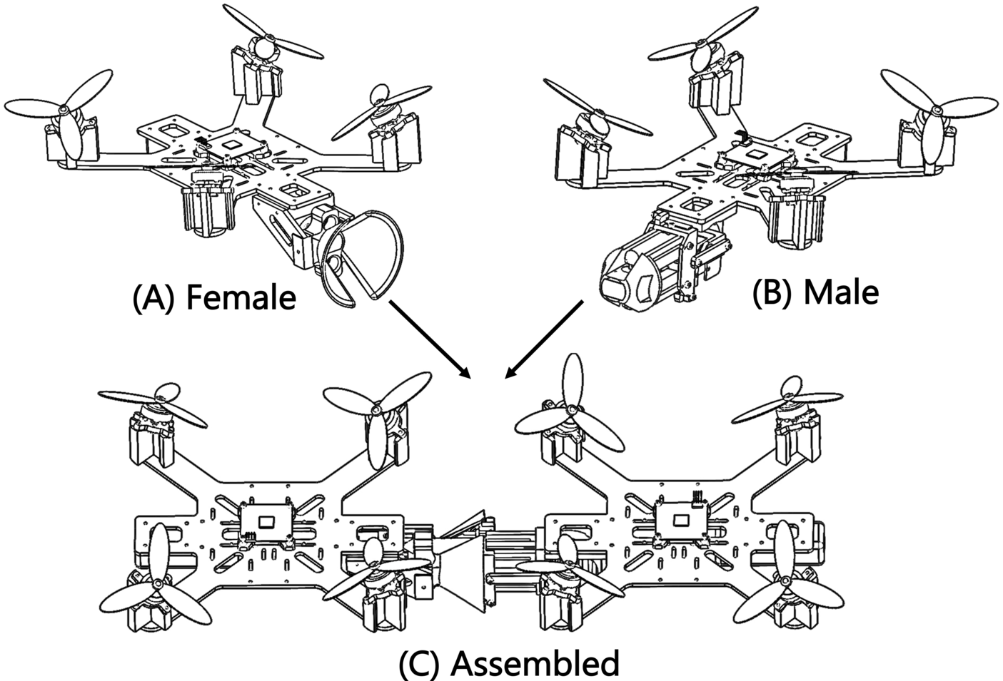
Figure 3: TRADY’s entire design. (A)Female unit. (B)Male unit. (C)Assembled state.

II-B Docking Mechanism

The prerequisites for the design of a docking mechanism are twofold: firstly, it should be capable of accomplishing both docking and undocking operations in the air, and secondly, it should possess sufficient rigidity to execute high-load tasks. Therefore, we propose a methodology of coupling with a permanent magnet and movable pegs.

II-B1 Female side

As shown in Fig. 4, the main components of the female mechanism are a permanent magnet equipped with a magnetic switching mechanism and a mechanism called a drogue, which compensates for positioning errors.

The on-off switching of the magnetic force is realized by the principle illustrated in the cut model in Fig. 4. In this mechanism, it is possible to interrupt the magnetic force by rotating one of the two permanent magnets $180\text{\,}\mathrm{d}\mathrm{e}\mathrm{g}$ using a servo motor. Since the two magnets do not directly touch each other, the force that hinders the rotation of the magnet is only friction with the housing, and rotation is easily possible with a low-torque servo motor. Through the use of this magnet, restraint in the translational direction of the docking mechanism is achieved.

Furthermore, the drogue attached to the tip of the female mechanism is a mechanism adopted in autonomous aerial refueling systems for fighter aircraft such as [31], [32], which compensates for control errors of the size corresponding to the diameter of the mechanism. In this study, the radius of the drogue was set to $5\text{\,}\mathrm{c}\mathrm{m}$ in order to absorb errors within $\pm$$2.5\text{\,}\mathrm{c}\mathrm{m}$. Additionally, the gradient inside the drogue was empirically determined to be approximately $35\text{\,}\mathrm{d}\mathrm{e}\mathrm{g}$. The drogue not only compensates for position errors, but also has two additional functions. One is to improve rigidity by increasing the contact area, and the other is to prevent the influence of external magnetic forces by covering the magnets.

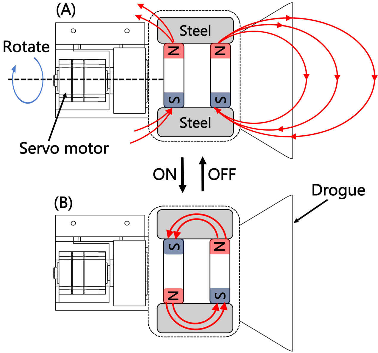
Figure 4: How the female mechanism works. In (A), since the magnetic force lines of force extend beyond the system, magnetic forces acts on the outside. In (B), magnetic force does not act on the outsinde because the magnetic lines of force circulate within the system. Note that the size of the switchable magnet is exaggerated in the depiction.

II-B2 Male side

As shown in Fig. 5, the male mechanism is composed of an steel plate for magnetic attraction and movable pegs. The movement of the peg is achieved using a slider-crank mechanism powered by a servo motor, and during docking, the peg is inserted into the receptor of the female mechanism to provide confinement in the bending direction. The tip of the mechanism is designed to closely adhere to the drogue of the female mechanism.

The overall size of the docking mechanism is determined based on the clearance that should be maintained between the rotors in the assembly state.

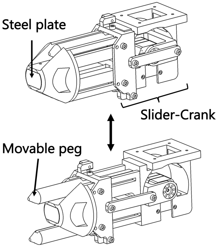
Figure 5: How the male mechanism works. The pegs are driven by the slider-crank mechanism and inserted into female mechanism.

III Modeling and Rotor Configuration

In this section, we introduce the kinematics and dynamics model of our robot in the first place, followed by the thrust allocation. Then, we present the method of optimization of rotor configuration.

III-A Modeling

TABLE I: Definition of physical quantities for multirotor.

Symbol	Definition
$n$	Number of rotors
$m$	Mass of body
$\bm{I}$	Moment of inertia ob body
{W}	World coordinates
{CoG}	CoG coordinates
$\bm{r}$	Position of CoG
$\bm{R}$	Rotation matrics of body
$\bm{\alpha}=[\begin{array}[]{ccc}\theta&\phi&\psi\\ \end{array}]$	Euler angles (roll, pitch, yaw)
$\bm{p_{i}}$	Position of i-th rotor
$\bm{u_{i}}$	Direction of i-th rotor( $\|\bm{u_{i}}\|=1$)
$\bm{\lambda}=^{t}\![\lambda_{1},\lambda_{2},\cdots,\lambda_{N}]$	Thrust
$\bm{\sigma}=[\sigma_{1},\sigma_{2},\cdots,\sigma_{N}]$	Counter torque of each rotor
$\bm{f}$	Resultant force
$\bm{\tau}$	Resultant torque
$\bm{\omega}$	Angular velociy
$\bm{g}=[\begin{array}[]{ccc}0&0&g\\ \end{array}]$	Acceleration ofGravity

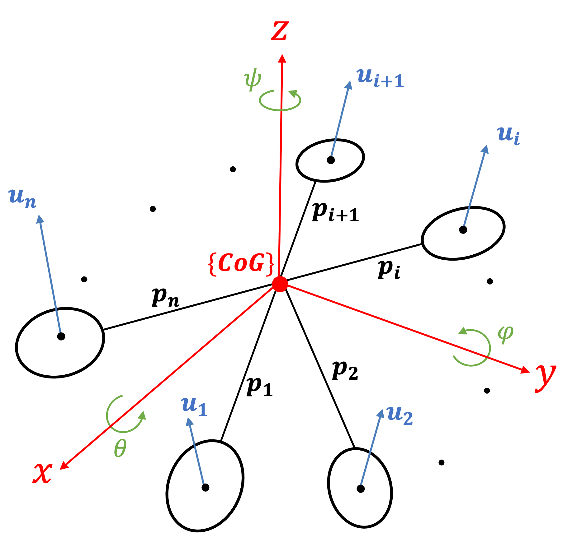
(A)

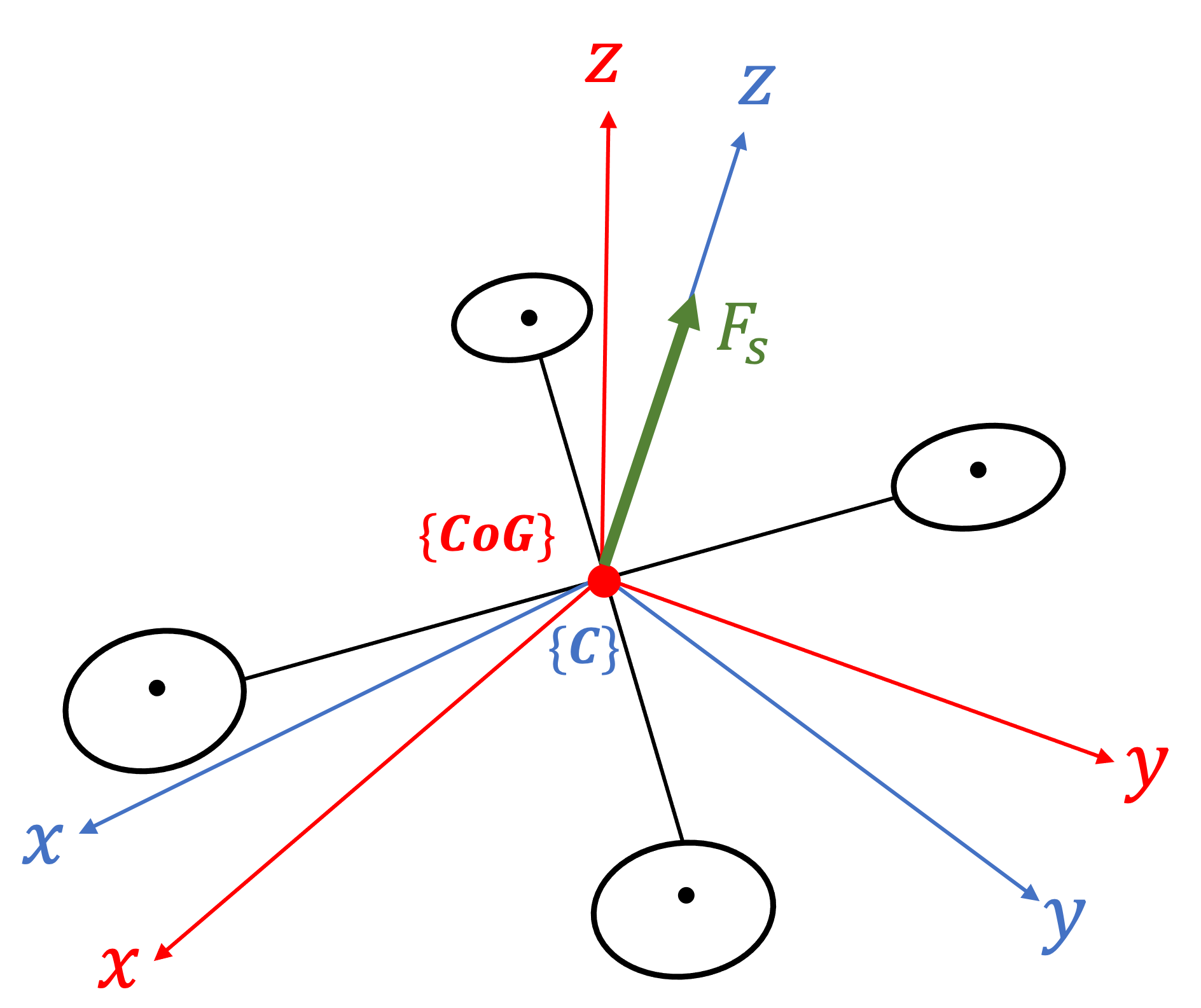
(B)

Figure 6: (A)Multi-rotor kinematics model with any number of rotors. The number of rotors is denoted by $n$; in this study, $n=8$ in the assemble state and $n=4$ for a unit. The frame ${\{CoG\}}$ have the origin at the center-of-mass of the whole model and z-axis is oriented vertically to airframe. (B)Relationship between ${\{CoG\}}$ and ${\{C\}}$. $\bm{F_{z}}$ in the figure is the resultant rotor thrusts force when the robot is hovering.

The kinematics model of TRADY is depicted in Fig. 6(A) and each quantities are difined as shown in Table. I. Since this model can be applied to multirotors with any number of rotors, the model of TRADY is represented by Fig. 6 with $n=4$ in the unitary state, and with $n=8$ in the assembly state.

Based on this kinematics model, the wrench-force ${}^{\{{CoG}\}}\bm{f}$ and torque ${}^{\{{CoG}\}}\bm{\tau}$ ) can be written as

$${}^{\{{CoG}\}}\bm{f}=\sum\limits_{i=1}^{n}\lambda_{i}{}^{\{{CoG}\}}\bm{u}_{i},$$ (1)

$${}^{\{{CoG}\}}\bm{\tau}=\sum\limits_{i=1}^{n}\lambda_{i}{}^{\{{CoG}\}}\bm{p}_{i}\times{}^{\{{CoG}\}}\bm{u}_{i}+\bm{\sigma}{}^{\{{CoG}\}}\bm{f},$$ (2)

where ${\{{CoG}\}}$ is the frame that have the origin at the center-of-mass of the body. From (1) and (2), the translational and rotational dynamics of a multirotor unit are given by the Newton-Euler equation as followings:

$$M{}^{\{W\}}\ddot{\bm{r}}_{\{CoG\}}={}^{\{W\}}\bm{R}_{\{CoG\}}{}^{\{{CoG}\}}\bm{f}+\left(\begin{array}[]{c}0\\ 0\\ -Mg\end{array}\right),$$ (3)

$$\begin{split}{}^{\{{CoG}\}}\bm{I}{}^{\{{CoG}\}}\dot{\bm{\omega}}&={}^{\{{CoG}\}}\bm{\tau}+\bm{\sigma}{}^{\{{CoG}\}}\bm{f}\\ &\quad-{}^{\{{CoG}\}}\bm{\omega}\times{}^{\{{CoG}\}}\bm{I}{}^{\{{CoG}\}}\bm{\omega},\end{split}$$ (4)

where ${\{W\}}$ frame represent the world coordinate system. Then, using (1) and (2), allocation from the thrust force $\bm{\lambda}$ to the resultant wrench can be given by following:

$$\left(\begin{array}[]{c}{}^{\{{CoG}\}}\bm{f}\\ {}^{\{{CoG}\}}\bm{\tau}\end{array}\right)=\left(\begin{array}[]{c}\bm{Q_{tran}}\\ \bm{Q_{rot}}\end{array}\right)\bm{\lambda}=\bm{Q}\bm{\lambda},$$ (5)

where

$$\bm{Q_{tran}}=\left({}^{\{{CoG}\}}\bm{u}_{1},{}^{\{{CoG}\}}\bm{u}_{2},\cdots,{}^{\{{CoG}\}}\bm{u}_{n}\right),$$ (6)

$$\bm{Q_{rot}}=\left({}^{\{{CoG}\}}\bm{v}_{1},{}^{\{{CoG}\}}\bm{v}_{2},\cdots,{}^{\{{CoG}\}}\bm{v}_{n}\right),$$ (7)

$${}^{\{{CoG}\}}\bm{v}_{i}={}^{\{{CoG}\}}\bm{p}_{i}\times{}^{\{{CoG}\}}\bm{u}_{i}.$$ (8)

Note that the second term in (2) is omitted for the remainder of the analysis because it is one order of magnitude smaller than the first term in general.

III-B Thrust Allocation

III-B1 In the Assembly State

In the assembly state, TRADY is fully-actuated, and the allocation matrics $\bm{Q}$ is full-rank. Therefore, we can gain MP pseudo-inverse matrics $\bm{{}^{\#}Q}$. Given a desired wrench, the target thrust can be computed by following:

$$\bm{\lambda}\>=\>\bm{{}^{\#}Q}\left(\begin{array}[]{c}{}^{\{{CoG}\}}\bm{f}\\ {}^{\{{CoG}\}}\bm{\tau}\end{array}\right).$$ (9)

III-B2 In the Unitary State

In the unitary state, $\bm{Q}\in R^{6\times 4}$ is rank deficient, and we need to adopt under-actuated model. As the conventional method, the control targets for under-actuated model are $f_{z}$, $\tau_{x}$, $\tau_{y}$, and $\tau_{z}$. Applying the control method illustrated in Section. IV, we can achieve the hovering of a quadrotor unit with these four inputs. In the case of a quadrotor with non-tilted rotors, because it does not produce $f_{x}$ and $f_{y}$, desired thrusts are easily calcurated as following:

$$\bm{\lambda}\>=\>\bm{{}^{\#}\left({}^{quad}Q\right)}{\>}^{t}[\begin{array}[]{cccc}f_{z}&\tau_{x}&\tau_{y}&\tau_{z}\end{array}],$$ (10)

where

$$\bm{{}^{quad}Q}\>=\>\left(\begin{array}[]{c}\bm{Q_{tran,z}}\\ \bm{Q_{rot}}\end{array}\right)\in R^{4\times 4},$$ (11)

and $\bm{Q_{tran,z}}\in R^{1\times 4}$ is the third row vector of $\bm{Q_{tran}}$.

However, TRADY unit is a tilted quadrotor that produces translation forces $f_{x}$, $f_{y}$ and these are uncontrollable with (10). Therefore, assuming the existence of the static thrust $\bm{\lambda_{s}}$ that enables hovering while suppressing the generation of $f_{x}$ and $f_{y}$, we introduce a method to apply (10) to the thrust allocation of tilted quadrotor by utilizing $\bm{\lambda_{s}}$.

In [33], Zhao et al. use a tilted coodinate system in order to obtain $\bm{\lambda_{s}}$ and we apply this idea to our work. Now, we introduce a new coodinate system ${\{{C}\}}$ that has the origin at the center-of-mass of body as shown in Fig. 6(B). Furthermore, we define ${\{{C}\}}$ to fulfill the following conditions:

$$\bm{Q_{tran}}^{\prime}\bm{\lambda_{s}}=-m\bm{g},$$ (12)

$$\bm{Q_{rot}}^{\prime}\bm{\lambda_{s}}=\bm{0},$$ (13)

where $\bm{Q_{tran}}^{\prime}$, $\bm{Q_{rot}}^{\prime}$ are allocation matrices defined in ${\{{C}\}}$.
(12), (13) indicate that the direction of the resultant force due to $\bm{\lambda_{s}}$ coincides with the z-axis of ${\{{C}\}}$. In other word, by controlling the robot’s attitude so that ${\{{C}\}}$ is horizontal, it becomes possible to hover the robot without generating excess forces in the horizontal direction. In this case, by using $\bm{Q_{tran}}^{\prime}$ and $\bm{Q_{rot}}^{\prime}$, thrust allocation can be achieved through (10), similar to that of a non-tilt quadrotor. Therefore, we focus on deriving $\bm{Q_{tran}}^{\prime}$, $\bm{Q_{rot}}^{\prime}$, and ${\{{C}\}}$.

Since both ${\{{C}\}}$ and ${\{{CoG}\}}$ have origins at the center-of-mass, from (13), following is also satisfied:

$$\bm{Q_{rot}}\bm{\lambda_{s}}=0.$$ (14)

Additionally, regarding translation, following is valid from (12):

$$\|\bm{F_{z}}\|=mg,$$ (15)

where $\bm{F_{z}}=\bm{Q_{trans}}\bm{\lambda_{s}}$. Then, we difine the rotation matrics $\bm{R_{C}}$ that satisfies:

$$\bm{R_{C}}\bm{F_{z}}={}^{t}[\begin{array}[]{ccc}0&0&mg\end{array}].$$ (16)

Integrating (14), (15), and (16) we can gain follows:

$$\bm{R_{C}}\left(\begin{array}[]{c}\bm{Q_{tran}}\\ \bm{Q_{rot}}\end{array}\right)\bm{\lambda_{s}}={}^{t}[\begin{array}[]{cccccc}0&0&mg&0&0&0\end{array}].$$ (17)

Comparing (12) and (13) with (17), our discussion results in followings:

$$\bm{R_{C}}\bm{Q_{tran}}=\bm{Q_{tran}}^{\prime},$$ (18)

$$\bm{R_{C}}\bm{Q_{rot}}=\bm{Q_{rot}}^{\prime}.$$ (19)

Because (18), (19) mean that $\bm{R_{C}}$ is the rotation matrics that maps ${\{{CoG}\}}$ to ${\{{C}\}}$, the conversion from ${\{{CoG}\}}$ to ${\{{C}\}}$ is easily calcurated with $\bm{R_{C}}$. Furthermore, (12) to (19) suggest that if there exists a $\bm{Q}$ that satisfies (12) and (13) for a given $\bm{\lambda_{s}}$, it is possible to hover tilted quadrotor using that $\bm{\lambda_{s}}$.

III-C Optimized Rotor Configuration

The TRADY rotor configuration must meet three prerequisites. Firstly, it must enable fully-actuated model control in the assembly state. Secondly, it should allow for under-actuated model control in the unitary state. Finally, it must attain the necessary flight properties required for aerial assembly/disassembly motion. Therefore, we propose a methodology to optimize the rotor configuration that satidsfies these conditions.

III-C1 Fully-actuated Model Controllability

Initially, we propose a technique for achieving fully-actuated model control when TRADY is in the assembly state. As described in Equation 1, the full rank of matrix $\bm{Q}$ is equivalent to fully-actuated model control, as $\bm{Q}$ can map L to an arbitrary wrench in real space if it is full rank. However, each rotor has a limit of thrust force, which can lead to instability of control due to weak resultant force or torque in certain directions. Thus, rather than directly employing algebraic methods to make $\bm{Q}$ full rank, we seek to maximize the available force and torque region to ensure translational and rotational controllability in all axes. To accomplish this, a concept of feasible control force convex polyhedron $\mathcal{V}_{\mathcal{F}}$, and torque convex polyhedron $\mathcal{V}_{\mathcal{T}}$ were introduced by [34]. These are defined as follows:

$$\mathcal{V}_{\mathcal{F}}\left(\bm{U}\right):=\left\{{}^{\{{CoG}\}}\bm{f}\in R^{3}\mid 0\leq\lambda_{i}\leq\lambda_{\max}\right\},$$ (20)

$$\mathcal{V}_{\mathcal{T}}\left(\bm{U}\right):=\left\{{}^{\{{CoG}\}}\bm{\tau}\in{R}^{3}\mid 0\leq\lambda_{i}\leq\lambda_{\max}\right\},$$ (21)

where the set of rotor direction vectors $\bm{U}$ is defined as $\bm{U}=[\begin{array}[]{ccc}\bm{u_{1}}&\cdots&\bm{u_{8}}\\ \end{array}]$. In addition, ${}^{\{{CoG}\}}\bm{f}$, ${}^{\{{CoG}\}}\bm{\tau}$ are defined in (1), (2) and maximum thrust for each rotor in TRADY is denoted by $\lambda_{\max}$, while the minimum thrust is established at 0, as we utilize unidirectional rotors.

Then, we define the values for the guaranteed minimum control force, denoted as $f_{min}$, and the corresponding torque, represented by $\tau_{min}$, in accordance with the subsequent equations are being satisfied:

$$\|{}^{\{{CoG}\}}\bm{f}-m\bm{g}\|\leq f_{min}\>\Rightarrow\>{}^{\{{CoG}\}}\bm{f}\in\mathcal{V}_{\mathcal{F}},$$ (22)

$$\|{}^{\{{CoG}\}}\bm{\tau}\|\leq\tau_{min}\>\Rightarrow\>{}^{\{{CoG}\}}\bm{\tau}\in\mathcal{V}_{\mathcal{T}}.$$ (23)

Note that our robot is controled under the premise that the roll and pitch angles are proximate to zero. As such, we posit that the gravity force is horizontal to the CoG frame, and we account for this force as an offset when defining the guaranteed control force.

Therefore, by maximizing these $f_{min}$ and $\tau_{min}$, the guaranteed force and torque regions can be maximized. Thus, we initially explicate the methodology for computing $f_{min}$. As an example of feasible control force convex polyhedron which is depicted in Fig. 7, $f_{min}$ is equal to the radius of the inscribed sphere of this polyhedron, and the same is true for torque. Thereby, $f_{min}$ is calculated by exploiting the distance $d^{f}_{ij}\left(\bm{U}\right)$, which is the length from the origin to a plane of polyhedron along its normal vector $\bm{h^{f}_{ij}}$.

The calculation of $d^{f}_{ij}\left(\bm{U}\right)$ can be performed as following.

$$d_{ij}^{f}\left(\bm{U}\right)=\left|\sum_{k=1}^{N}\max\left(0,\lambda_{\max}\>^{t}\bm{h^{f}_{ij}}{}^{\{{CoG}\}}\bm{u_{k}}\right)-\>^{t}\bm{h^{f}_{ij}}m\boldsymbol{g}\right|,$$ (24)

where

$$\bm{h^{f}_{ij}}=\frac{{}^{\{{CoG}\}}\bm{u_{i}}\times{}^{\{{CoG}\}}\bm{u_{j}}}{\left|{}^{\{{CoG}\}}\bm{u_{i}}\times{}^{\{{CoG}\}}\bm{u_{j}}\right|}\>\>.$$ (25)

Moreover, as $f_{min}$ corresponds to the radius of the inscribed sphere, we may ascertain $f_{min}$ in the following manner:

$$f_{min}=\min_{i,j}d_{ij}^{f}.$$ (26)

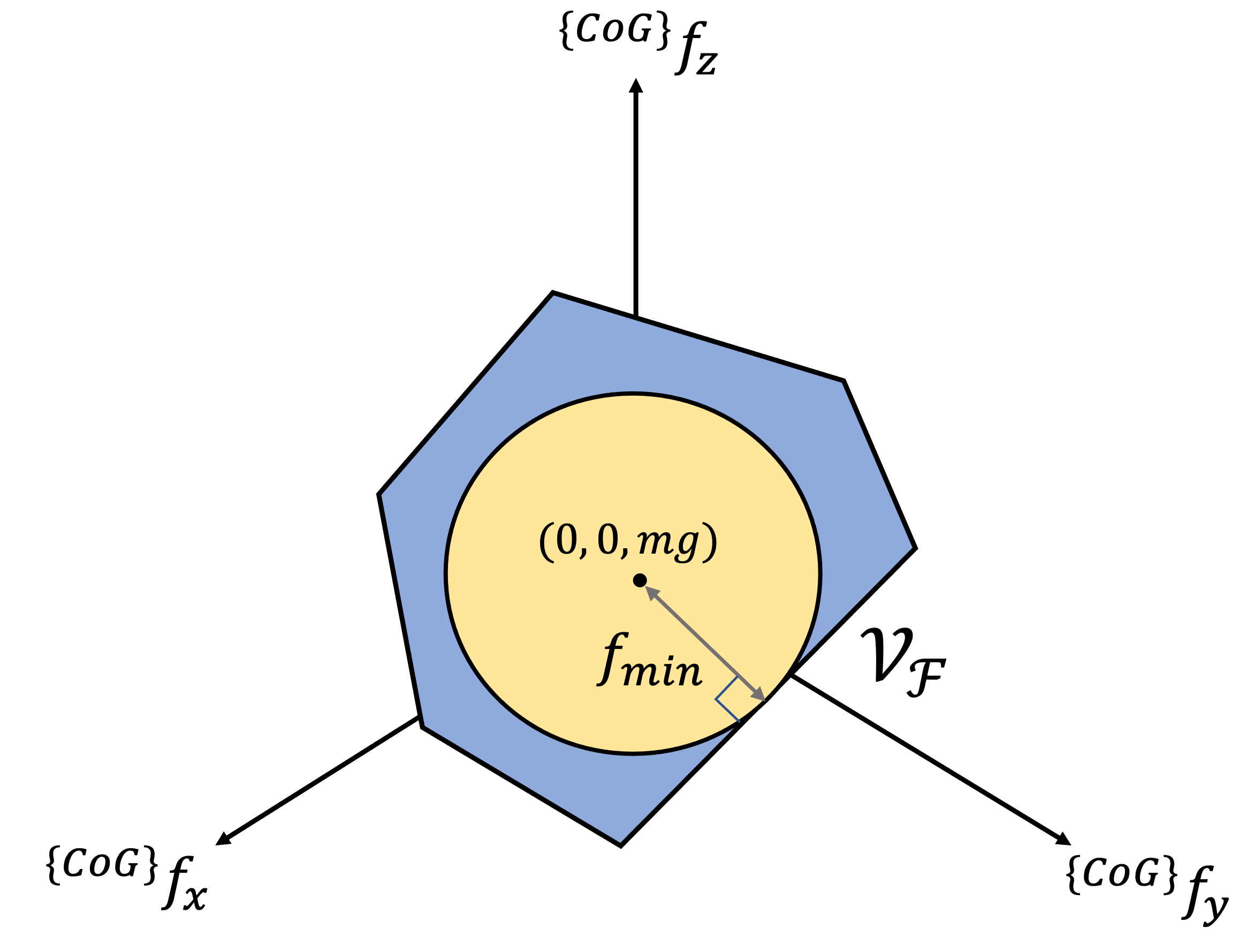
Figure 7: The example of a feasible control force convex polyhedron defined in (20). The blue region in this figure is $\mathcal{V}_{\mathcal{F}}$ , and ${}^{\{{CoG}\}}\bm{f}$ in the yellow region satisfies the left side of (22).

Note that, if $f_{min}>0$, the robot can fly.

Similarly, $\bm{\tau_{min}}$ can be acquired by calculating $d_{ij}^{\tau}$ in the following manner.

$$d_{ij}^{\tau}\left(\bm{U}\right)=\left|\sum_{k=1}^{N}\max\left(0,\lambda_{\max}\>{}^{t}\bm{h^{\tau}_{ij}}{}^{\{{CoG}\}}\bm{v_{k}}\right)\right|,$$ (27)

$$\tau_{min}=\min_{i,j}d_{ij}^{\tau},$$ (28)

where

$$\bm{h^{\tau}_{ij}}=\frac{{}^{\{{CoG}\}}\bm{v_{i}}\times{}^{\{{CoG}\}}\bm{v_{j}}}{\left|{}^{\{{CoG}\}}\bm{v_{i}}\times{}^{\{{CoG}\}}\bm{v_{j}}\right|}\>\>.$$ (29)

To sum up, the objective function to be maximized in this optimization of TRADY’s rotor configuration is formulated as follows.

$$S\left(\bm{U}\right)=w_{1}f_{min}+w_{2}\tau_{min},$$ (30)

where $w_{1}$ and $w_{2}$ are the positive weights to balance between force and torque. Additionally, the constraints can be expressed as follows:

$$\bm{\ast 1}: f_{min}>0,$$ (31)

$$\bm{\ast 2}: \tau_{min}>0.$$ (32)

Although our primary focus is on the assembled aircraft consisting of two quadrotor units, the maximization of $S\left(\bm{U}\right)$ within the constraints described in (31) and (32) ensures the attainment of fully-actuated model control in aircraft composed of an arbitrary number of units.

III-C2 Under-actuated Model Controllability

Subsequently, we present the constraints for (30) to enable TRADY to achieve stable flight in the unitary state. Firstly, as previously noted in Section. I, the TRADY is composed of two quadrotor units, each possessing an identical rotor configuration. Consequently, the whole structure can be illustrated as Fig. 8(A), with a constraint expressed as follows:

$$\bm{u_{1}}=\bm{u_{5}},\bm{u_{2}}=\bm{u_{6}},\bm{u_{3}}=\bm{u_{7}},\bm{u_{4}}=\bm{u_{8}}.$$ (33)

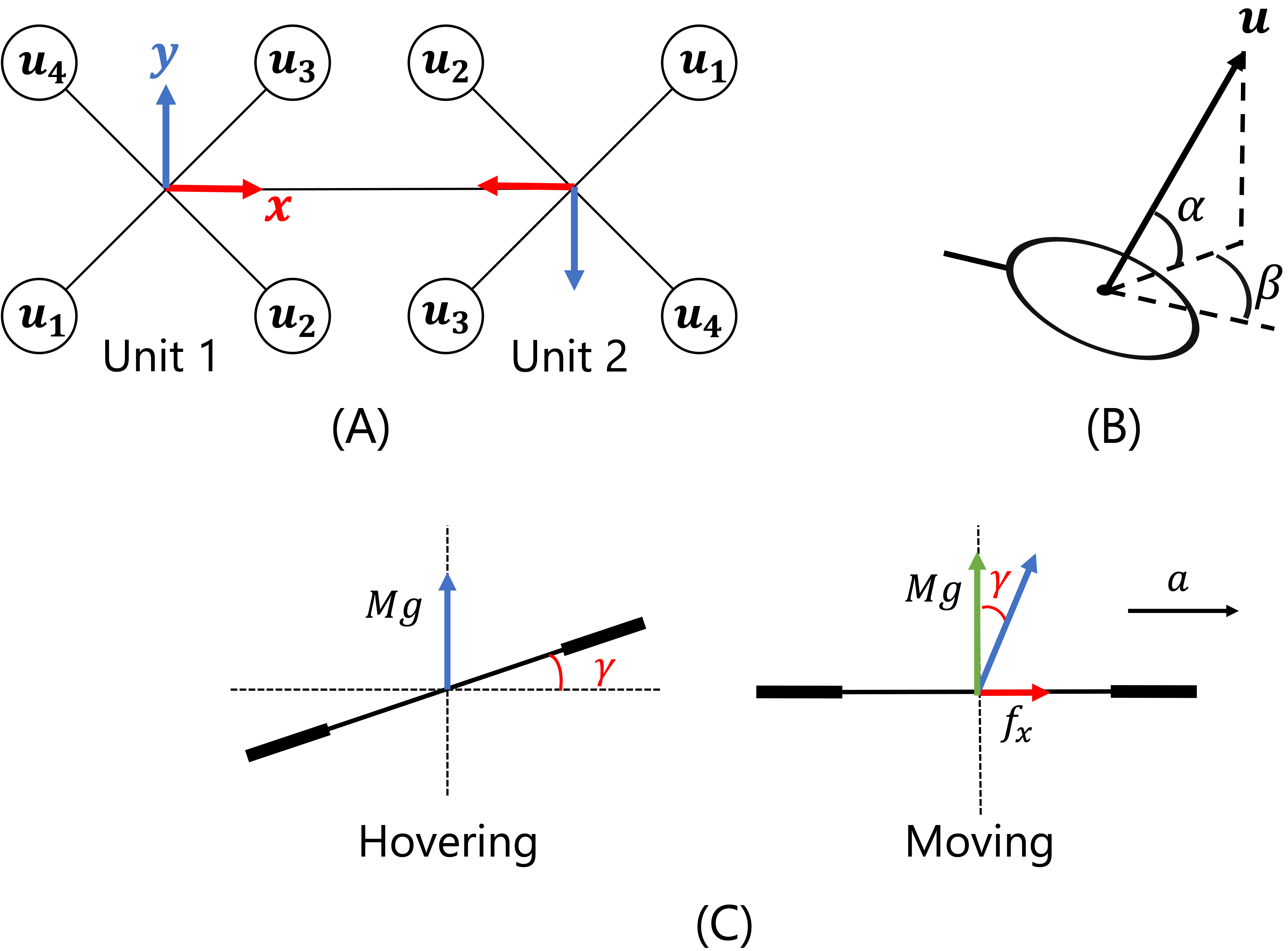
Figure 8: (A)Overall configuration of TRADY in its assembled state. In this configuration, each docking mechanism is mounted on the same position of the unit.(B)Rotor direction vector $\bm{u}$ represented by spherical coordinate parameters $\alpha$ and $\beta$. (C)Airframe inclination during hovering and movement.

Additionally, as noted above, the prerequisite for stable flight of the units is that both (14) and (15) are satisfied. Despite the presence of an infinite number of combinations for ${\{{C}\}}$ and $\bm{\lambda_{s}}$, we assume that $\bm{\lambda_{s}}=\lambda_{s}\;{}^{t}[\begin{array}[]{cccc}1&1&1&1\\ \end{array}]$, to ensure even distribution of workload across each rotor. Consequently, an additional constraint can be formulated as follows.

$$\bm{\ast 3}: \|\lambda_{s}\bm{Q_{trans}}\;{}^{t}[\begin{array}[]{cccc}1&1&1&1\\ \end{array}]\;\|=mg,$$ (34)

$$\bm{\ast 4}: \lambda_{s}\bm{Q_{rot}}\;{}^{t}[\begin{array}[]{cccc}1&1&1&1\\ \end{array}]=\bm{0}.$$ (35)

III-C3 Flight Characteristics for Aerial Assembly/Disassembly

Next, we consider the flight characteristics required for aerial assembly/disassembly. Generally, quadrotors obtain translational propulsion by inclining their airframe. However, this inclination impedes parallel contact between two units during assembly motion. The coupling mechanism proposed in this study has a small contact area, which renders this non-parallel relationship a hindrance to the assembly process.

However, in the instance of the TRADY unit, its target coordinate system is ${\{{C}\}}$, which is inclined with respect to ${\{{CoG}\}}$. Consequently, the airframe inclines during hovering, and conversely, it assumes a horizontal orientation during movement in a specified direction. Hence, we establish a novel constraint for the optimization to regulate the tilted angle of ${\{{C}\}}$ in such a way that the airframe assumes a horizontal orientation when it accelerates along the positive x-axis direction in Fig. 8(B).

Assuming that the inclination angle during hovering is $-\gamma$ as shown in Fig. 8(C), the force exerted by the unit in the x-direction when it is in a horizontal state can be written as $mg\tan\gamma$. Then the desired value of $\gamma$ is calculated as follows:

$$\gamma=-\tan^{-1}\left(\frac{{}^{des}a}{g}\right),$$ (36)

where ${}^{des}a$ is the target acceleration in the x-direction. Consequently, we introduce the following constraint condition for the rotation matrix $\bm{R_{C}}$, to ensure that ${\{{C}\}}$ tilts by $-\gamma$ around the y-axis:

$$\bm{\ast 5}: \bm{R_{c}}=\left[\begin{array}[]{ccc}\cos\left(-\gamma\right)&0&\sin\left(-\gamma\right)\\ 0&1&0\\ -\sin\left(-\gamma\right)&0&\cos\left(-\gamma\right)\\ \end{array}\right].$$ (37)

To sum up, the optimization problem for the rotor configuration can be summarized as follows:

$$\underset{\bm{U}}{\text{maximize}} S\left(\bm{U}\right)$$ (38)

subject to $$\bm{\ast 1}\sim\bm{\ast 5}$$

III-C4 Solver for Optimization Problem

Finally, in order to solve the designed optimization problem, it is necessary to choose an algorithm, but it is not always guaranteed that a solution that satisfies all the set constraints exists. Therefore, we use the global optimization algorithm ISRES [35] that can find the closest possible solution even if a perfect solution is not found. The optimized $\bm{U}$ obtained as a result of solving the optimization problem using the parameters shown in Table. II and the guaranteed minimum force and torque in the unitary and assembly states are presented in Table. III. Here, each $\bm{u}$ is represented by spherical coordinate parameters $\alpha$ and $\beta$ as shown in Fig. 8(B). Furthermore, the outcomes are rounded off to two significant digits. The obtained outcome reveals that the optimized rotor angles exhibit a symmetrical pattern. This occurrence can be attributed to the constraints established in (34) and (35), as these equations embody force and torque offsets. In addition to this, it can be seen that both the minimum guaranteed force and torque become more than twice as high in the assembly state when using fully-actuated model compared to the unitary state.

TABLE II: Parameters for optimization.

Parameter	Value
Mass of a unit	$1.1\text{\,}\mathrm{k}\mathrm{g}$
Coordinates of rotors	$\left(\pm\>0.12\>\text{m},\pm\>0.12\>\text{m}\right)$
Maximum thrust of rotor	$7\text{\,}\mathrm{N}$
Coefficient of counter-torque	$-0.011\text{\,}{\mathrm{m}}^{-1}$
${}^{des}a$	$1\text{\,}\mathrm{m}\mathrm{/}\mathrm{s}^{2}$

TABLE III: Result optimization.

Parameter	Value
$[\alpha_{1},\;\beta_{1}]$	[0.45 rad,  0.73 rad]
$[\alpha_{2},\;\beta_{2}]$	[0.52 rad,  -2.1 rad]
$[\alpha_{3},\;\beta_{3}]$	[0.52 rad,  2.1 rad]
$[\alpha_{4},\;\beta_{4}]$	[0.45 rad,  -0.73 rad]
$f_{min,\>unit}$	$3.1\text{\,}\mathrm{N}$
$\tau_{min,\>unit}$	$0.64\text{\,}\mathrm{N}\mathrm{m}$
$f_{min,\>assem}$	$7.5\text{\,}\mathrm{N}$
$\tau_{min,\>assem}$	$2.8\text{\,}\mathrm{N}\mathrm{m}$

IV Control

Firstly, we outline the methodology for flight control, which incorporates fully-actuated model control for the unitary state and fully-actuated model control for the assembly state. Next, we propose a system switching strategy to be executed during the docking or undocking process.

IV-A Fully-actuated Flight Control

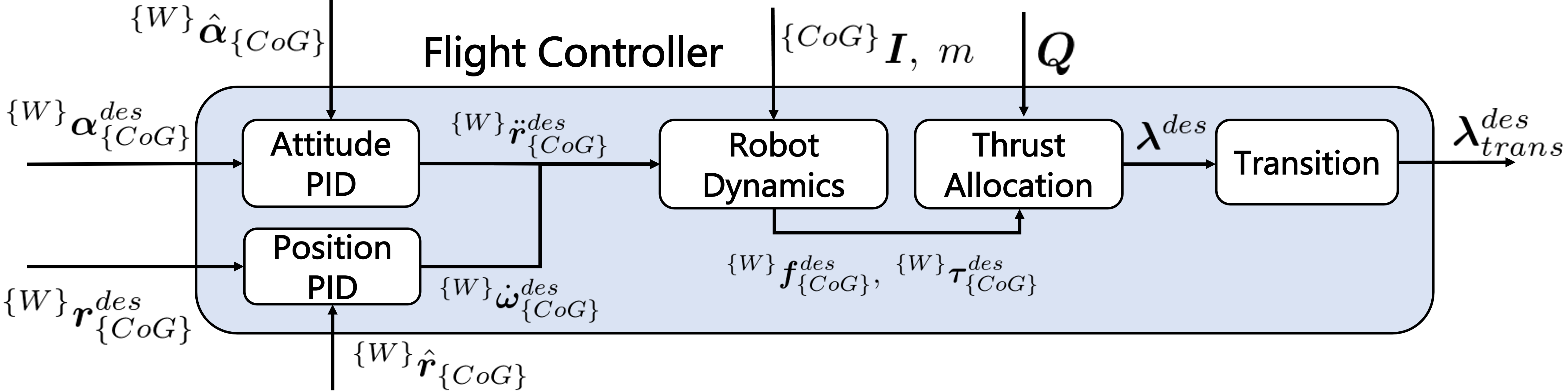
Figure 9: Block diagram of fully-actuated controller. The blue rectangle represents the processing flow of the controller, while the incoming arrows from other components shown in Fig. 11 denote parameter transmission. The “Robot Dynamics” in this diagram refers to the Newton-Euler equations described in (3) and (4), and “Thrust allocation” is the computation based on the pseudoinverse matrix, as described in (9). Additionally, “Transition” is the state transition process defined by equation 3.

IV-A1 Position Control

For position control, a general PID controller is adopted. Thus, from (1), (2), the desired force and torque can be derived as following:

$$\bm{f}^{des}=m\;{}^{\{W\}}\bm{R}_{\{CoG\}}^{-1}\left(\bm{K_{p}}\bm{e_{r}}+\bm{K_{i}}\int\bm{e_{r}}dt+\bm{K_{d}}\dot{\bm{e_{r}}}\right),$$ (39)

where $\bm{e_{r}}$ is a position error defined as $\bm{e_{r}}={}^{\{W\}}\bm{r}^{des}_{\{CoG\}}-{}^{\{W\}}\bm{r}_{\{CoG\}}$, and $\bm{K_{p}}$, $\bm{K_{i}}$, $\bm{K_{d}}$ are gains for controller. Additionally, ${\{C\}}$ is used instead of ${\{CoG\}}$ in the unitary state.

In the assembly state, as shown in Fig. 9, the obtained $\bm{f}^{des}$ from (39) is allocated to the desired thrust by $\bm{Q_{trans}}$.

IV-A2 Attitude Control

Next, we explain attitude control. In the case of a fully-actuated model, it is possible to apply traditional PID control for attitude control. Here, by using (2), the desired torque can be obtained as follows:

$$\begin{split}\bm{\tau}^{des}=\;{}^{\{{CoG}\}}\bm{I}\left(\bm{K_{p}}\bm{e_{\alpha}}+\bm{K_{i}}\int\bm{e_{\alpha}}dt+\;\bm{K_{d}}\dot{\bm{e_{\alpha}}}\right)\\ +{}^{\{{CoG}\}}\bm{\omega}\times\;{}^{\{{CoG}\}}\bm{I}\;{}^{\{{CoG}\}}\bm{\omega},\end{split}$$ (40)

where $\bm{e_{\alpha}}$ is an attitude error defined as $\bm{e_{\alpha}}={}^{\{W\}}\bm{\alpha}^{des}_{\{{CoG}\}}-{}^{\{W\}}\bm{\alpha}_{\{{CoG}\}}$ and $\bm{K_{p}}$, $\bm{K_{i}}$, $\bm{K_{d}}$ are gains for controller. Then, the desired torque $\bm{\tau}^{des}$ obtained from attitude control is allocated into the desired thrust for each rotor using the allocation matrix $\bm{Q_{rot}}$ as shown in Fig. 9.

IV-B Under-actuated Flight Control

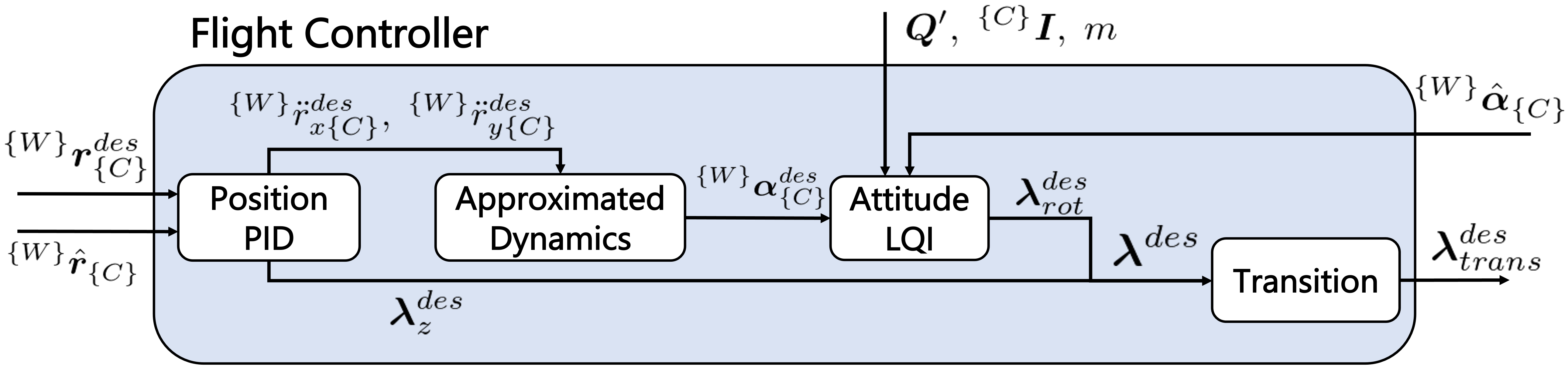
Figure 10: Block diagram of under-actuated controller. “Approximated Dynamics” in this diagram represents the operation of converting the target acceleration to the target attitude through the approximation of the horizontal state described by (41) and (42). In addition, $\bm{\lambda_{z}}^{des}$ is actually the output of “Position PID” converted to thrust by (44).

IV-B1 Position Control

The position control for the underactuated model is developed using the methodology presented in [36], which involves determining the target force via conventional PID feedback loop and subsequently converting it to target roll and pitch angles. The target forces $f^{des}_{x}$ and $f^{des}_{y}$ can be obtained using (39), followed by determining the target roll $\theta$ and pitch $\phi$ as outlined below:

$${}^{\{W\}}\theta^{des}_{\{C\}}=atan^{-1}\left(-f_{y},\sqrt{f^{2}_{x}+f^{2}_{z}}\right),$$ (41)

$${}^{\{W\}}\phi^{des}_{\{C\}}=atan^{-1}\left(f^{2}_{x},f^{2}_{z}\right).$$ (42)

These target angles are achieved by attitude controller.

Additionally, regarding the position control in z-direction, collctive thrust force $f^{des}_{z}$ is calculated in the following manner:

$$f^{des}_{z}=^{t}\left({}^{\{W\}}\bm{R}_{\{C\}}\bm{b}\right)\bm{f}^{des},$$ (43)

where $\bm{b}$ is a unit vector ${}^{t}\left[\begin{array}[]{ccc}0&0&1\\ \end{array}\right]$.

Then, using $\bm{\lambda_{s}}$ defined in (12) and (13), the target thrust for z-directional control is calculated as follows:

$$\bm{\lambda}^{des}_{z}=\frac{f^{des}_{z}}{mg}\bm{\lambda}_{s}.$$ (44)

IV-B2 Attitude Control

In attitude control, to suppresse the uncontrollable horizontal forces due to the tilted rotors, we adopt LQI control[37] which is a type of optimal control that derives control inputs that minimize the cost function. Therefore, by designing the cost function appropriately, various requirements can be met in addition to convergence speed. The state equation of posture control is described as follows:

$$\bm{\dot{x}}=\bm{A}\bm{x}+\bm{B}\bm{\lambda}+\bm{D}\left(\;{}^{\{C\}}\bm{I}^{-1}\;{}^{\{C\}}\bm{\omega}\times\;{}^{\{C\}}\bm{I}\;{}^{\{C\}}\bm{\omega}\right),$$

$$\bm{y}=\bm{C}\bm{x},$$ (45)

where

$$\bm{x}=\;^{t}\left[\begin{array}[]{ccccccccc}e_{x}&\dot{e_{x}}&e_{y}&\dot{e_{y}}&e_{z}&\dot{e_{z}}&\int{e_{x}}&\int{e_{y}}&\int{e_{z}}\end{array}\right],$$ (47)

$$\bm{e}=\bm{\alpha}^{des}-\bm{\alpha},$$

$$\bm{\dot{e}}=\dot{\bm{\alpha}}^{des}-\dot{\bm{\alpha}},$$

$$\bm{B}=\;^{t}\left[\begin{array}[]{ccccccc}\bm{0_{4\times 1}}&\bm{B_{1}}&\bm{0_{4\times 1}}&\bm{B_{2}}&\bm{0_{4\times 1}}&\bm{B_{3}}&\bm{0_{4\times 3}}\\ \end{array}\right],$$ (49)

$$\left[\begin{array}[]{ccc}\bm{B_{1}}&\bm{B_{2}}&\bm{B_{3}}\\ \end{array}\right]=\;^{t}\left({}^{\{C\}}\bm{I}^{-1}\bm{Q_{rot}}^{\prime}\right).$$ (51)

Note that the target roll and pitch angle is ${}^{\{W\}}\theta_{\{C\}}$, ${}^{\{W\}}\phi_{\{C\}}$ obtained from (41) and (42). In regards to the cost function, this study designs a function with the objective of improving convergence, suppressing the control input, and suppressing translational forces. In this case, the cost function is given as follows:

$$J=\int_{0}^{\infty}\left(\;{}^{t}\bm{x}\bm{M}\bm{x}+\;^{t}\bm{\lambda}\bm{N}\bm{\lambda}\right)dt,$$ (52)

where $\bm{M}$ and $\bm{N}$ are diagonal weight matrices. The first term in (52) corresponds to the control output’s norm, and minimizing this norm can enhance the convergence. Moreover, concerning the second term in (52), the method of defining $\bm{N}$ as follows has been proposed in [33]:

$$\bm{N}=\bm{W_{1}}+\bm{Q_{trans}}^{T}\;{}^{\prime}\bm{W_{2}}\bm{Q_{trans}}^{\prime},$$ (53)

where $\bm{W_{1}}$ and $\bm{W_{2}}$ are also diagonal weight matrices. Then, the first term of (53) creates a quadratic form ${}^{t}\bm{\lambda}\bm{N}\bm{\lambda}$ when substituted into (52), corresponding to the norm of control input. Therefore, by minimizing this term, the control input can be suppressed. Furthermore, when the second term is substituted into (52), the following equation is derived.

$$^{t}\bm{\lambda}\;^{t}\bm{Q_{trans}}^{\prime}\bm{Q_{trans}}^{\prime}\bm{\lambda}=\;^{t}\bm{f}\bm{f}=\|\bm{f}\|^{2}.$$ (54)

As seen from (54), the norm of translational force is represented by the second term of (53). Therefore, by employing the control input $\bm{\lambda}$ that minimizes the cost function defined in (52), stable attitude control of a unit equipped with tilted rotors can be achieved. By solving the algebraic Riccati equations derived from (IV-B2) and (52), we obtain the feedback gain $\bm{K}$. Therefore, the desired $\bm{\lambda}$ is calculated as follows:

$$\bm{\lambda}^{des}_{rot}=\bm{K}\bm{x}+{}^{\#}\bm{Q_{rot}}^{\prime}\;{}^{\{C\}}\bm{\omega}\times\;{}^{\{C\}}\bm{I}\;{}^{\{C\}}\bm{\omega}.$$ (55)

Finally, in combination with the $z$ axis position control, the final output in the unitary state is ultimately calculated as follows:

$$\bm{\lambda}^{des}=\bm{\lambda}^{des}_{z}+\bm{\lambda}^{des}_{rot}.$$ (56)

IV-C System Switching

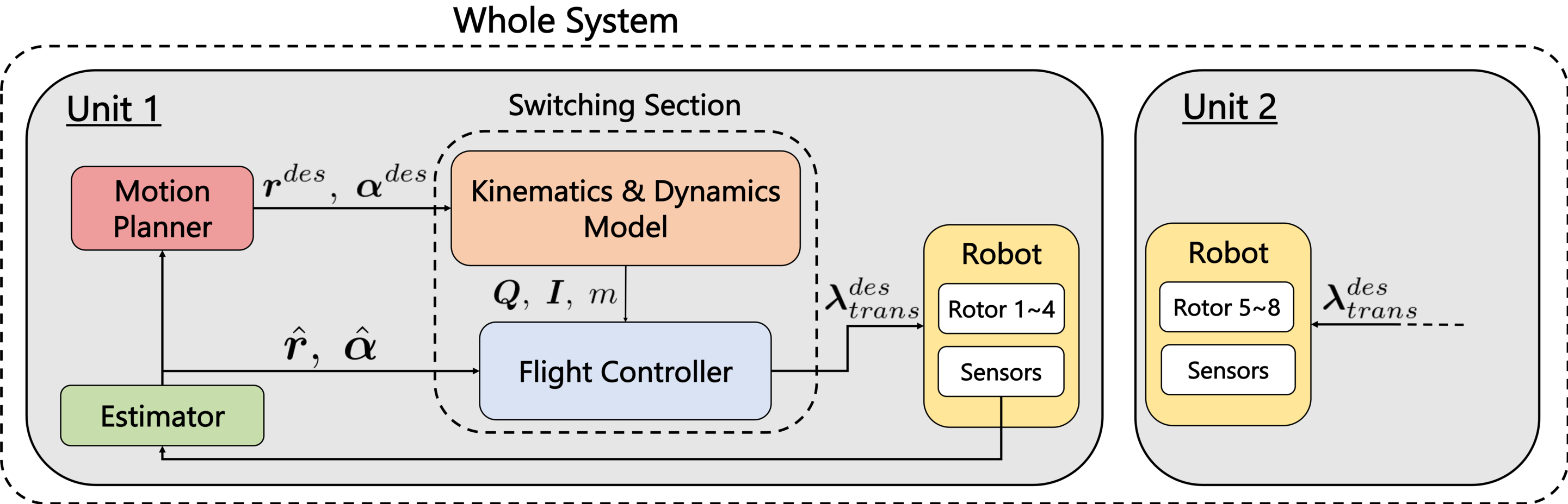
Figure 11: Overall system diagram of the control system. The “Estimator” in the figure processes various sensor values using a Kalman filter to perform self-state estimation. Additionally, the “Motion Planner” sends position and attitude commands for assembling/disassembling actions and aerial task realization. The “Switching Section” is a partition that switches between the assembly state and the unitary state, which includes the “Kinematics & Dynamics Model” and “Flight Controller”. The “Kinematics & Dynamics Model” outputs the inertia values of the aircraft and $\bm{Q}$ in the case of under-actuated or fully-actuated model, while the “Flight Controller” is shown in Fig. 9 and Fig. 10. Even in the assembly state, the units do not communicate with each other and independently control their respective rotors.

We present a methodology for system switching that is executed during assembling and disassembling actions.

IV-C1 Overall Control System

To begin with, the overall control system is designed, as depicted in Fig. 11. The “Motion Planner”, “Estimator”, and “Robot” sections adopt common processes in both the assembly state and the unitary state. Conversely, the “Switching Section” serves as a partition that alternates between the assembly and unitary states. During the assembly state, the entire system is controlled by a distributed control system, while each unit controls its respective rotors based on a common robot model without communicating with one another. Therefore, the overall structure of the system remains unchanged between the assembly state and the unitary state, with only the contents of the “Switching Section” being switched.

IV-C2 Transition Process

Next, we explain the transition process that should be performed when switching systems. The problem when switching the system is the model error related to the inertia values and rotor performance of the robot. In normal flight control of TRADY, model errors are compensated for by the integral term of PID and LQI. In addition, there is no offset thrust based on default values in the gravity direction, and it is all compensated for by the integral term. Model error compensation by integral value is gradually performed while gradually increasing the rotor thrusts during takeoff, so it is generally completed until hovering.

As an example, we consider the system switching during the assembly action. When switching the system, most control values are reset because the controller is switched. However, as mentioned earlier, gravity compensation is performed by the integral term, so only the integral terms are carried over in order to continue the flight. However, since this integral term compensates for the model error of the robot in the unitary state, the model error in the assembly state is not compensated for. Model errors that suddenly occur during flight, unlike during takeoff, cause discrete increases or decreases in rotor thrusts, which have a significant negative effect on control stability.

To address this issue, a method of gradually transitioning rotor thrusts while compensating for the model error of the assembly state model was developed. Although it is impossible to predict each rotor thrust after model error compensation, the total weight of the system does not change before and after system switching, thereby the total thrust force acting in the gravity direction after model error compensation can be said to be the same as in the unitary state. Furthermore, since among each rotor thrust, the proportion that works in the direction of gravity does not change, consequently, the total thrust of all rotors can be said to be equal before and after switching. Therefore, the influence of sudden model errors can be suppressed by scaling the rotor thrusts output from the controller based on the total thrust in the unitary state. However, it is necessary to reflect the influence of the control output in the assembly state, thereby the control output is scaled using the value obtained by superimposing the total thrust in these two states.

Here, the total thrust in the unitary state is obtained using the total thrust immediately before the system switch, and the total thrust in the assembly state is obtained using the real-time control output. Then, rotor thrusts during the transition is scaled as follows:

$$\bm{\lambda^{des}_{trans}}=\frac{S_{trans}}{S_{assem}}\bm{\lambda^{des}_{assem}},$$ (57)

$$S_{trans}=W\left(t\right)S_{assem}+\left(1-W\left(t\right)\right)S_{unit},$$ (58)

where $S_{assem}$ is the total thrust in the assembly state defined as $S_{assem}=\sum\limits_{i=1}^{n}\|\bm{\lambda}^{des}_{assem,\;i}\|$ and $S_{unit}$ is that in the unitary state. Note that $S_{assem}$ is a variable but $S_{unit}$ is a constant because $S_{unit}$ competed by the thrust at the moment of switching. Additionally, $W\left(t\right)$ is the weight function used in the superimposing and it is desirable for it to smoothly converge to 1. Therefore, $W\left(t\right)$ is defined as follows:

$$W\left(t\right)=1-\frac{1}{at+1},$$ (59)

where $a$ is a constant and $t$ is a variable representing time. Then, $W\left(t\right)$ satisfies follows:

$$W\left(0\right)=0,$$

$$\lim_{t\to\infty}W\left(t\right)\to 1.$$ (60)

Therefore, in (58), initially the influence of $S_{unit}$ is dominant, but gradually $S_{assem}$ becomes dominant and ultimately $\bm{\lambda_{trans}}$ becomes indistinguishable from the normal output of the assembly state controller. Thus, as a result, even after the system switch, the rotor thrust transitions smoothly. The variable $a$ in (59) determines the convergence rate of the function, and in this work, it was empirically set to $a=0.9$. In this case, $W\left(t\right)$ attains a value of 0.99 when $t=120$. During actual implementation, $W\left(t\right)$ is refreshed at each control cycle with a frequency of $0.025\text{\,}\mathrm{s}$. Consequently, $W\left(t\right)$ achieves 0.99 after approximately $3\text{\,}\mathrm{s}$ of real time have elapsed.

To sum up, by utilizing the aforementioned methodology, it is possible to address the discrete thrust changes caused by model errors during system switching. This transition process occurs outside the controller, as illustrated in Fig. 9 and Fig. 10, and can be regarded as a kind of disturbance to the feedback loop. However, if this disturbance itself converges sufficiently quickly, the overall system stability is ultimately dependent on the stability of controllers. In the case of our method, the tuning of $a$ in (59) ensures the convergence rate of the transition process, while the stability of the PID controller is achieved through the tuning of its gains, and the stability of the LQI controller is guaranteed by (52). Therefore, the proposed transition process has no impact on the stability of the feedback loop.

V Motion Strategy

In this section, we introduce the motion strategy for executing assembly/disassembly motion in mid-air. Initially, we propose the overarching strategy, followed by an specific explication of each constituent.

V-A Overall Strategy

As explained in Section. II-B, in aerial assembly/disassembly motions, the two units come into extreme proximity, causing unstable flight. This makes high-precision position control difficult. Therefore, a motion strategy is required that ensures the certainty of the motion under multiple conditions, and executes it only if these conditions are met. Then, in this study, we divide the target action into several stages and represent them as an Finite State Machine (FSM) as shown in Fig. 12. In this FSM, conditions are set to transition between states, and when two units fulfill them, the motion transitions to the next state. By repeating this process, it becomes possible to autonomously perform aerial assembly/disassembly motion while avoiding hazardous conditions.

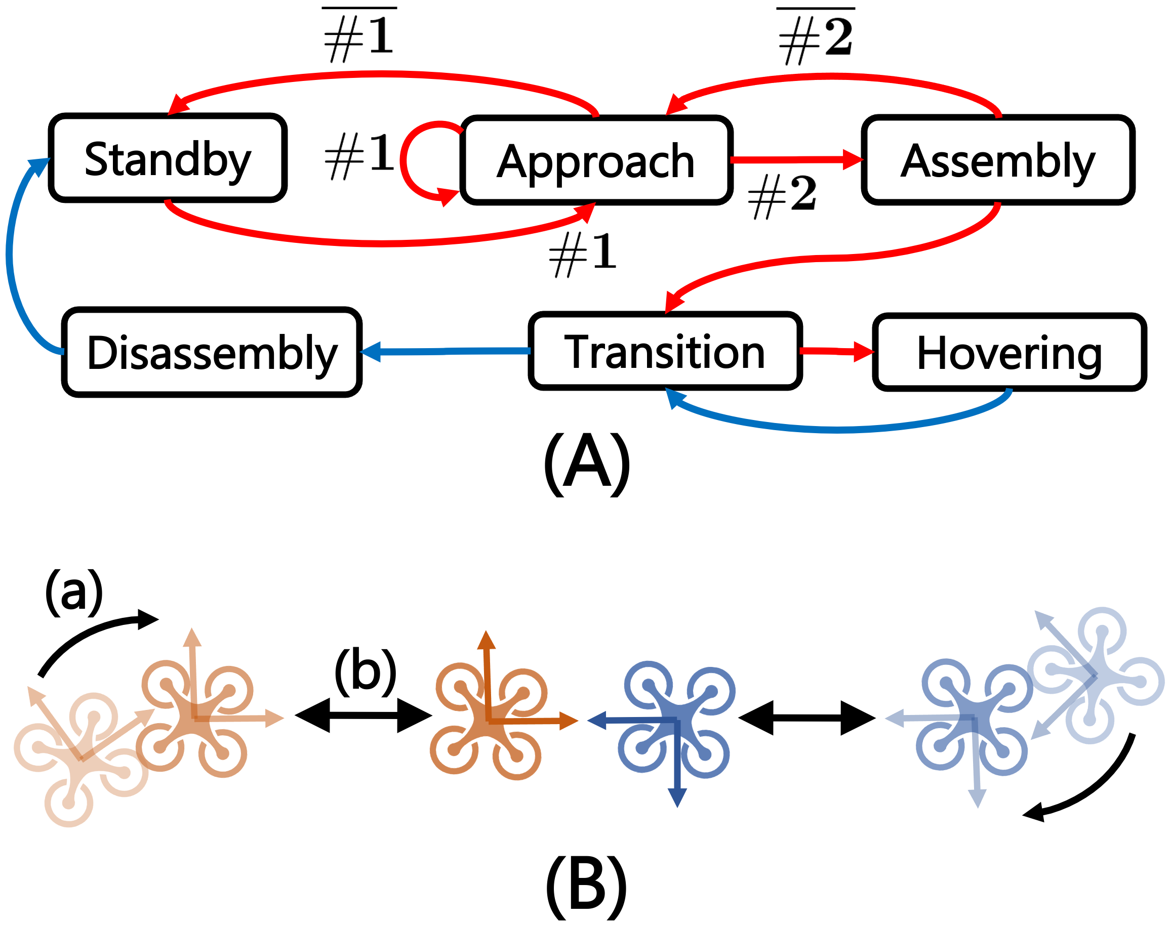
Figure 12: (A)The Finite State Machine for assembly/disassembly motion: Each block represents a corresponding state.The red arrows represent the transitions between the states for assembly, while the blue ones represent that for disassembly. Note that $\overline{\bm{\#}}$ represents the negation of $\bm{\#}$. (B)The procedure of assembly motion based on proposed strategy. Arrow (a) symbolizes the transition into the “Standby”, whereas arrow (b) signifies the iterative transitions into the “Approach” and “Standby” states.

V-B Assembly Motion

Now, we explain each state in the FSM, focusing on the assembly motion.

V-B1 Standby State

This state is the initial state of the FSM, where both units are guided towards their respective standby positions and yaw angles. The female unit maintains its position and yaw angle at the start of assembly, while the male unit is guided to a position and yaw angle $\psi$ that satisfies the following relationship:

$${}^{\{F\}}\bm{r}_{\{M\}}=\;^{t}\left[\begin{array}[]{ccc}d^{st}&0&0\end{array}\right],$$ (62)

$${}^{\{F\}}\psi_{\{M\}}=-\pi$$ (63)

where${\{F\}}$ represents the ${\{C\}}$ frame of the female unit, while ${\{M\}}$ represent that of the male unit. Additionally, $d^{st}$ is the desired distance between two units’ CoG. Note that the direction of each axis is the same as that shown in Fig. 8.

Here, we define the following condition $\bm{\#1}$ with respect to the errors in $r_{y}$, $r_{z}$, and $\psi$:

$$\bm{\#1}: \left(\begin{array}[]{c}{}^{\{F\}}r_{y\{M\}}\\ {}^{\{F\}}r_{z\{M\}}\\ {}^{\{F\}}\psi_{\{M\}}\\ \end{array}\right)\leq\left(\begin{array}[]{c}e^{\#1}_{y}\\ e^{\#1}_{z}\\ e^{\#1}_{\psi}\\ \end{array}\right)$$ (64)

where $e^{\#1}_{y}$,$e^{\#1}_{z}$,$e^{\#1}_{\psi}$ are tolerable errors. Condition $\bm{\#1}$ is used as a criterion to determine if the positional relationship between the two units is safe. If the relationship between the female unit and the male unit satisfies $\bm{\#1}$, the state transitions to the “Approach” state.

V-B2 Approach State

At this state, the male unit moves towards the female unit, while the female unit maintains its position and angle. During the approach phase, if condition $\bm{\#1}$ is no longer met, the approach motion is interrupted and the system transitions to the “Standby” state. By virtue of this process, it becomes possible to instantaneously recover from a hazardous positional state between the two units and continue with the assembly motion unimpeded.

Here, we define the following condition $\bm{\#2}$ with respect to the errors in $r_{x}$, $r_{y}$, $r_{z}$, and $\psi$:

$$\bm{\#2}: \left(\begin{array}[]{c}{}^{\{F\}}r_{x\{M\}}\\ {}^{\{F\}}r_{y\{M\}}\\ {}^{\{F\}}r_{z\{M\}}\\ {}^{\{F\}}\psi_{\{M\}}\\ \end{array}\right)\leq\left(\begin{array}[]{c}e^{\#2}_{x}\\ e^{\#2}_{y}\\ e^{\#2}_{z}\\ e^{\#2}_{\psi}\\ \end{array}\right)$$ (65)

where $e^{\#2}_{x}$,$e^{\#2}_{y}$,$e^{\#2}_{z}$,$e^{\#1}_{\psi}$ are tolerable errors. Condition $\bm{\#2}$ is used as a criterion to determine if the two units are in a position where they can docking. If the condition $\bm{\#2}$ is satisfied, the state transitions to the “Assembly” state.

V-B3 Assembly State

In this state, initially, the docking mechanism is activated by turning on the magnet and inserting the pegs, and subsequently, the system is transitioned into the assembly mode. During the aforementioned movements, if condition $\bm{\#2}$ is no longer met, the movement is halted and the state transitions to the “Approach” state.

V-B4 Transition State

In this state, the process of transition presented in Section. IV-C is executed.

V-C Disassembly Motion

In the case of aerial disassembly, the system transitions from “Hovering” to “Transition,” and then proceeds to “Disassembly.” During “Disassembly,” the coupling mechanism is released, allowing the two units to separate. Unlike in assembly, positional control of the bodies is not critical during disassembly, and therefore, there are no conditions that must be satisfied for the state transitions.

VI Experiment

In this section, we first describe the robot platform utilized in each experiment. Next, we present the experimental results, which include the evaluation of flight stability in each state, aearil assembly and disassembly motion based on proposed control method and motion strategy, and object manipulation in the assembly state.

VI-A Robot Platform

VI-A1 Hardware

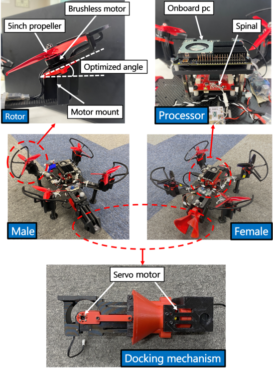
Figure 13: Hardware configuration of proposed robot TRADY.

Based on the design proposed in Section. II and Section. III, we introduce the hardware configuration illustrated in Fig. 13. The frame of the body is made of a $5\text{\,}\mathrm{m}\mathrm{m}$ CFRP plate, while the other parts are mainly made of PLA material. In determining the size of the entire body, we first determined the size of the docking mechanism based on the rigidity required for the coupling portion and then selected the minimum body size that can accommodate the docking mechanism.

The rotors are composed of 5 inch propellers (GEMFAN Hulkie 5055S-3) and brushless motors (ARRIS S2205), driven by ESC (T-Motor F45A). Each rotor is tilted based on the optimized $\bm{U}$ in Section. III. With this configuration, each rotor exerts a thrust of approximately $1\text{\,}\mathrm{N}$-$8\text{\,}\mathrm{N}$ at a voltage of $15\text{\,}\mathrm{V}$.

Furthermore, an on-board PC (Khadas VIM4) and a flight controller called Spinal, which uses an STM32 microcontroller, are installed on the body. The housing of the docking mechanism is made of PLA, and a servo motor (KONDO KRS-3302) is installed on both the male and female sides. In addition, Arduino nano is used to control the servo motor.

In addition, a $2200\text{\,}\mathrm{m}\mathrm{A}\mathrm{h}$ four-cell LiPo battery is used as the power source. However, in some experiments, power is supplied from a bground-based stabilizing power source instead of a battery to enable emergency stop.

Finally, Table. IV shows the characteristics of the robot.

TABLE IV: main parameters of robot

Parameter	Value
Mass of main body	$0.94\text{\,}\mathrm{k}\mathrm{g}$
Size of main body	$0.24\text{\,}\mathrm{m}$ $\times$$0.24\text{\,}\mathrm{m}$
Mass of docking mechanism (Male)	$0.16\text{\,}\mathrm{k}\mathrm{g}$
Mass of docking mechanism (Female)	$0.16\text{\,}\mathrm{k}\mathrm{g}$
Continuous flight time	$25\text{\,}\mathrm{m}\mathrm{i}\mathrm{n}$

VI-A2 Software

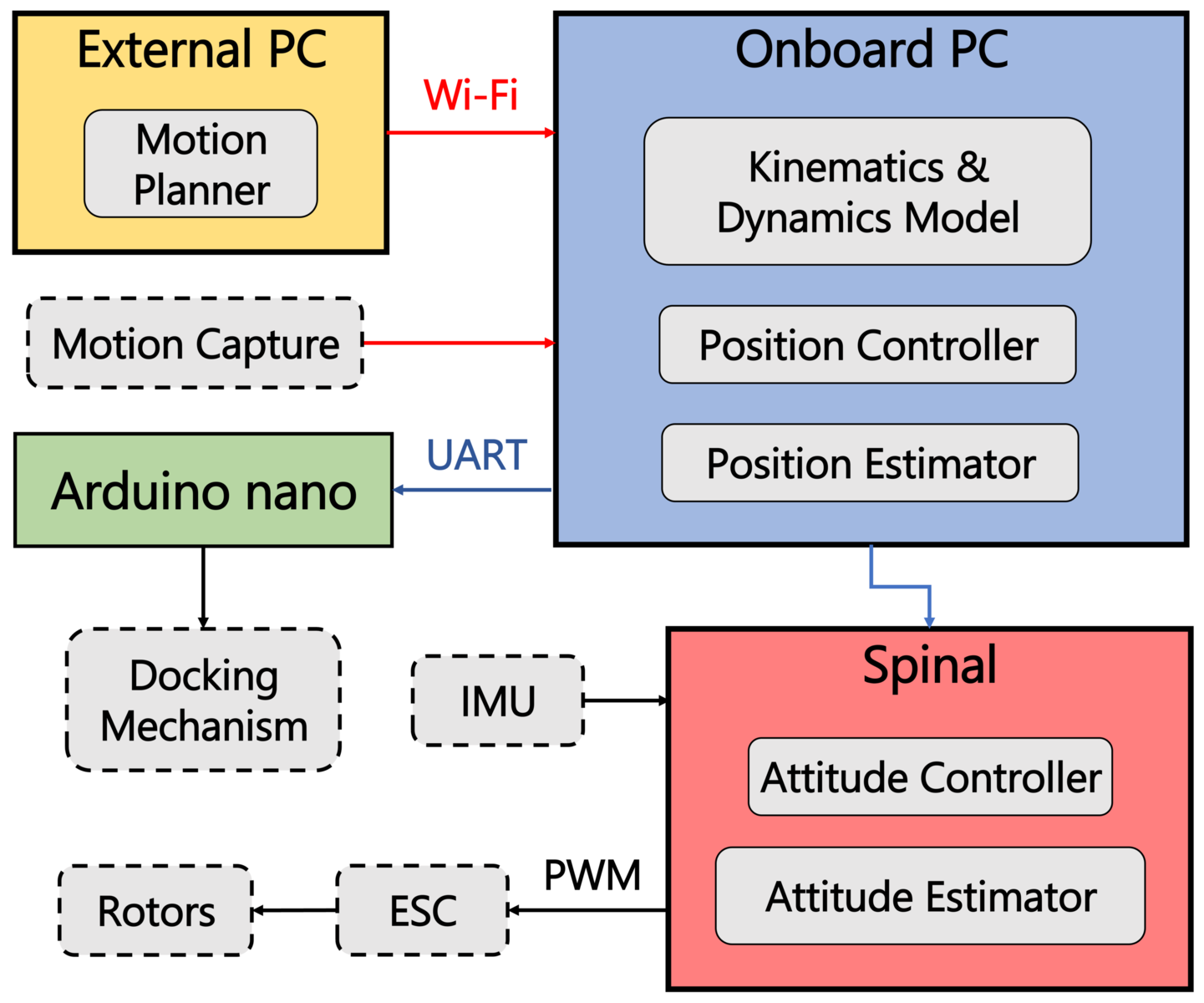
Figure 14: Communication system configuration of proposed robot TRADY.

Next, we introduce the communication system for proposed robot TRADY as shwon in Fig. 14. Firstly, the external PC executes motion planning including the strategy for the assembly/disassembly motion presented in Section. V, and it outputs position attitude commands. Subsequently, these commands are transmitted to the onboard PC through a Wi-Fi network. Furthermore, the external motion capture system transmits the positional state of the robot to the onboard PC. The onboard PC consists of a robot model calculation, position estimator by Kalman filter, and position controller. Afterward, the onboard PC transmits commands to Arduino and Spinal with UART communication. Spinal also receives self-attitude information from the IMU sensor and estimates the attitude of the robot with a Kalman filter. Target PWM is output from the attitude controller based on the estimated attitude values and commands from the onboard PC. Moreover, Arduino receives commands from the onboard PC and sends angle commands to the servo motors of the coupling mechanism.

VI-B Flight stability

We first conduct a circular trajectory tracking flight experiment in order to verify the flight stability of both the unitary state and the assembly state. In this experiment, a circular trajectory with a radius of $0.5\text{\,}\mathrm{m}$ at an altitude of $1\text{\,}\mathrm{m}$ was adopted, and a robot circles this obit twice in one minute. The result is shown in Fig. 15 and Table. V. Figure 1 visualizes the tracking error, while Table. V shows the Root Mean Squared Error (RMSE) from the trajectory for each state. From these results, it is found that both the under-actuated model control in the unitary state and the fully-actuated model control in the assembly state are possible. The control accuracy is inferior in the unitary state compared to the assembly state, which is due to not only the under-actuated model control but also the large moment of inertia of the body despite its weight. However, the positional error within this range can be dealt with by the drogue on the female-side docking mechanism and the proposed motion strategy, thus not posing significant issues.

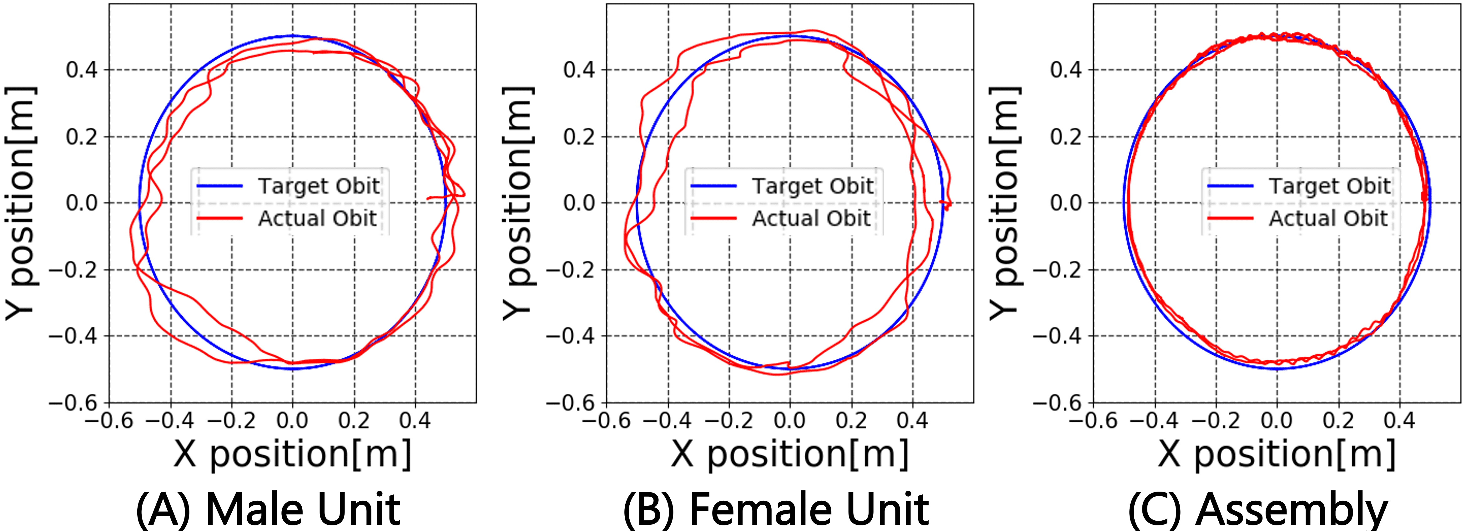
Figure 15: Visualized tracking error. The blue trajectory represents the target trajectory, while the red trajectory represents the actual trajectory.

TABLE V: errors from the desired trajectory

State	RSME
Male Unit	$3.5\text{\,}\mathrm{c}\mathrm{m}$
Female Female	$4.1\text{\,}\mathrm{c}\mathrm{m}$
Assembly	$0.83\text{\,}\mathrm{c}\mathrm{m}$

VI-C In-flight assembly and disassembly

VI-C1 Reliability of Aerial Assembly/Disassembly

To conduct an airborne coalescence experiment, the parameters in (64) and (65) must first be determined. The parameters $e^{\#1}_{y}$, $e^{\#1}_{z}$, $e^{\#1}_{\psi}$ in (64) are the criteria for determining the dangerous state, and therefore, smaller values of these parameters will result in more reliable merging, but will also increase the time required to complete the merging. Since the parameters $e^{\#2}_{x}$, $e^{\#2}_{y}$, $e^{\#2}_{z}$, $e^{\#2}_{\psi}$ in (65) are the criteria for docking certainty, there is also a tradeoff between certainty and time required to adjust these parameters. In this study, these values were adjusted through experiments on actual equipment, and the final values were determined as shown in Table. VI.

After determining the parameters, we conducted 15 experiments for both aerial assembly and disassembly. The results indicated a success rate of $86.7\text{\,}\%$ (13 successful attempts) for assembly behavior and a $100\text{\,}\%$ success rate (15 successful attempts) for disassembly behavior. In addition to this, the time required for the merging behavior ranged from $3\text{\,}\mathrm{s}$ to $15\text{\,}\mathrm{s}$, and there was a large variation. In two failed assembly experiments, the docking mechanism became stuck in a part of the airframe, making it impossible to transit from the “Approach” state to the “Standby” state, necessitating an emergency stop of the robot. As a solution to this issue, covering the entire unit body with a spherical guard would allow avoidance of contact between the docking mechanism and the airframe.

TABLE VI: parameter for motion strategy

Parameter	Value
$e^{\#1}_{y}$	$\pm$$0.02\text{\,}\mathrm{m}$
$e^{\#1}_{z}$	$\pm$$0.02\text{\,}\mathrm{m}$
$e^{\#1}_{\psi}$	$\pm$$0.13\text{\,}\mathrm{r}\mathrm{a}\mathrm{d}$
$e^{\#2}_{x}$	$\pm$$0.005\text{\,}\mathrm{m}$
$e^{\#2}_{y}$	$\pm$$0.01\text{\,}\mathrm{m}$
$e^{\#2}_{z}$	$\pm$$0.01\text{\,}\mathrm{m}$
$e^{\#2}_{\psi}$	$\pm$$0.01\text{\,}\mathrm{r}\mathrm{a}\mathrm{d}$
$d^{st}$	$0.6\text{\,}\mathrm{m}$

VI-C2 Stability of System Switching

Next, to evaluate the flight stability during the system switchover, we conducted in-flight assembly and disassembly experiments with and without the thrust transition method proposed in Section. Section. IV-C.

First, for the aerial assembly, the results with the transition process are shown in Fig. 16, and the results without the proposed thurst transition process are shown in Fig. 17. In the event of an increase in rotor thrust during the system switch, the forces in the x and y directions are offset; however, significant effects are apparent in the control of the z direction. Therefore, both Fig. 16 and Fig. 17 include plots of rotor thrust displacement and z-directional position error.

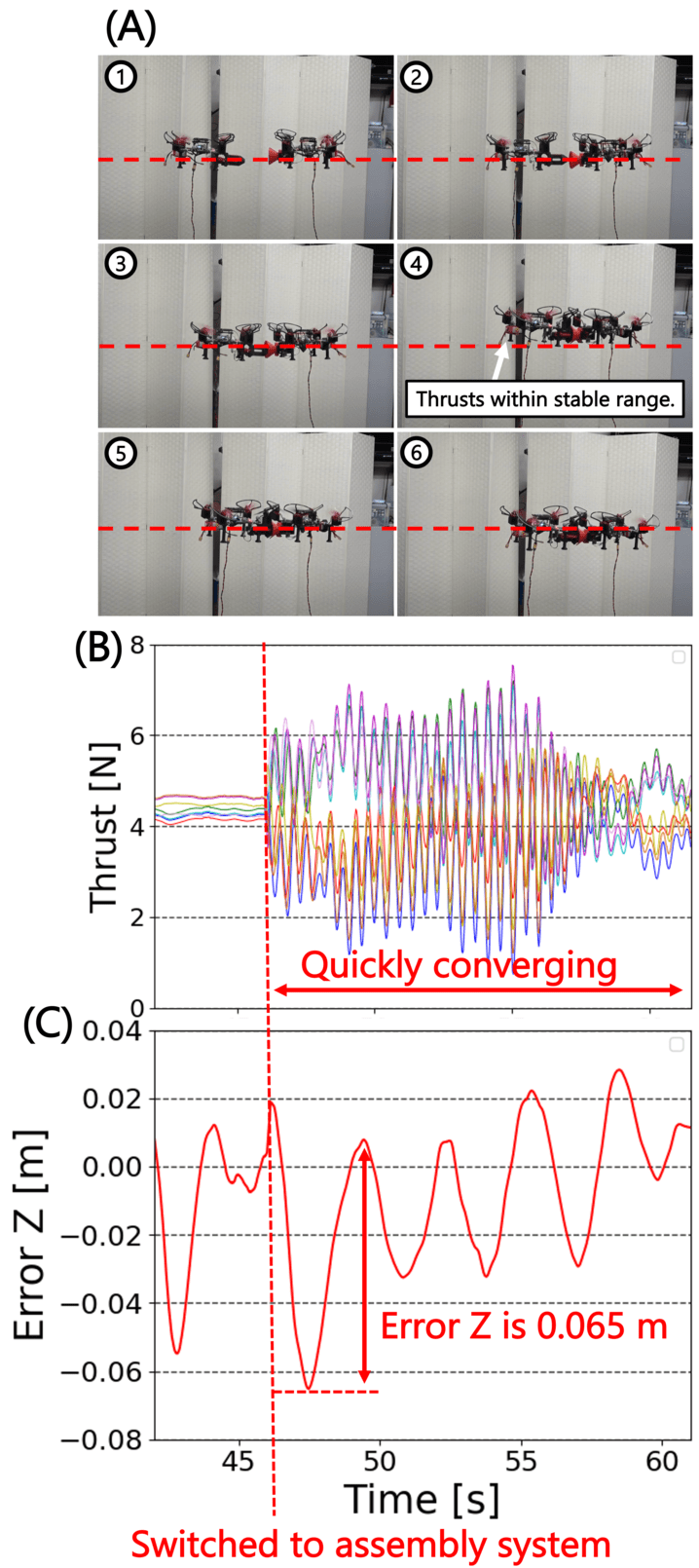
Figure 16: Result of aerial assembly with presented transition process. (A)Spapshots of aerial assembly motion and the red line in the figure represents target altitude. (B)Plot of the thrusts of 8 rotors during the motion. (C)Plot of the Error of altitude $z$ during the motion.

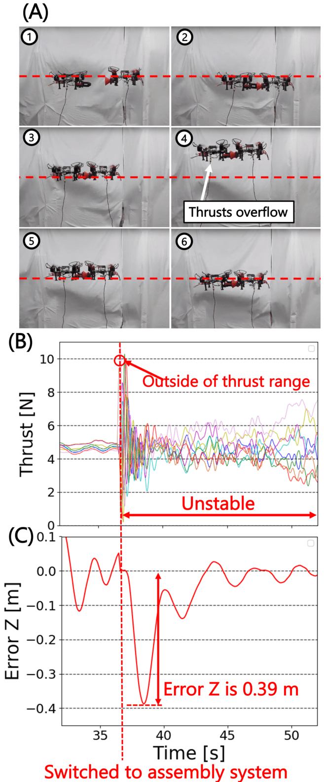
Figure 17: Result of aerial assembly without presented transition process.(A)-(B) are the same as those in Fig. 16.

Concerning the case of transition processing, it can be observed from Fig. 16 that stable aerial assembly and thrust transitions are achieved. As shown in Fig. 16(B) and (C), the total rotor thrust remains constant before and after the system switch, and the subsequent ascent of robot is limited to approximately $0.065\text{\,}\mathrm{m}$. Additionally, the control is rapidly stabilized following the switchover. Note that, despite the transition process, there are still discrete changes in the thrust of each rotor. However, these changes are due to alterations in the allocation of thrust to each rotor and not to model errors, and they have a negligible adverse effect on control performance.

On the contrary, regarding the experiment without transition processing, Fig. 17(B) shows that the target rotor thrust changed abruptly due to model errors that occur during the system switchover. The total rotor thrust increases by about $5\text{\,}\mathrm{N}$ before and after the switchover, and for some rotors the target thrust greatly exceeds the upper thrust limit. As a result, the robot rose about $0.39\text{\,}\mathrm{m}$ at a stretch immediately after assembly as show in Fig. 17(C), and unstable control continued after that.

These results indicate the efficacy of our proposed method for switching systems in aerial assembly motion.

Next, regarding aerial disassembly, Fig. 18 illustrates the experimental result of aerial disassembly with proposed transition process. Moreover, Fig. 19 illustrates the variation in rotor thrust before and after mid-air disassembly when the transition process was not applied. From these results, it was found that in aerial disassembly, it is possible to safely switch the system with or without transition processing. This is likely due to the fact that in the assembly state, decentralized control is performed by two controllers, resulting in model errors equivalent to those of two aircraft. In contrast, in the unitary state, only model errors equivalent to those of one aircraft are generated. As a result, in the unitary state, the effect of system switching on thrust is presumed to be small.

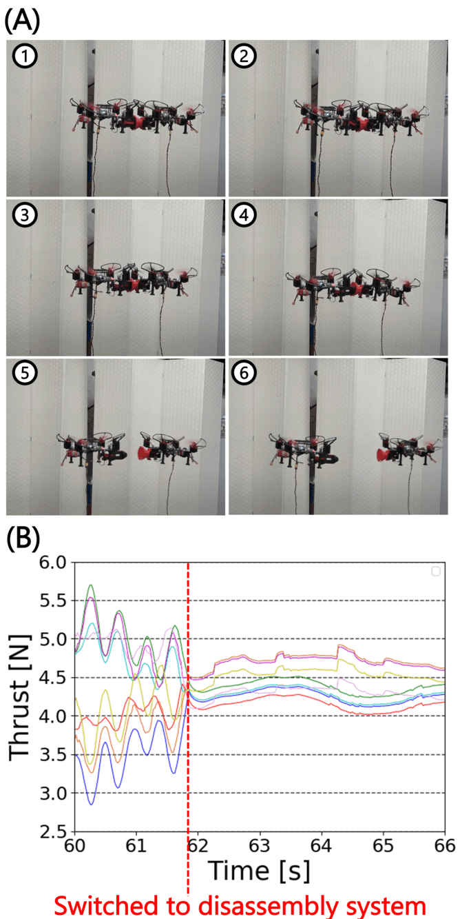
Figure 18: Result of aerial disassembly with the presented transition process.(A)Spapshots of aerial disassembly motion.(B)Plot of the thrusts of 8 rotors during the motion.

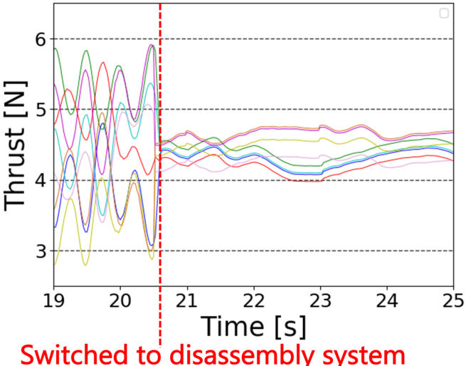
Figure 19: Plot of the thrusts of 8 rotors during the disassembly without transition process.

VI-D Peg Insertion

Next, we conducted an experiment to verify the aerial object manipulation ability in the assembly state. First, we conducted an experiment to insert a diameter of $6\text{\,}\mathrm{m}\mathrm{m}$ peg into a diameter of $25\text{\,}\mathrm{m}\mathrm{m}$ pipe as an analogy to drilling and Pic-and-Place tasks. Due to the requirement of high position accuracy and independent control of translation and rotation for this task, the fully-actuated model control is necessary. Note that in this study, we focus on the control performance of the robot, and therefore, the task is performed by manual operation, not by automatic control based on motion planning. The experimental results are shown in Fig. 20.

From these results, it was demonstrated that the robot can be maneuvered with an error of approximately $\pm$$1\text{\,}\mathrm{c}\mathrm{m}$. Furthermore, as shown in Fig. 20(B),(C), the pitch angle of the robot was kept within approximately $\pm 1.5$ degrees during movement and hovering, demonstrating translational control can be achieved while suppressing the impact on the attitude.

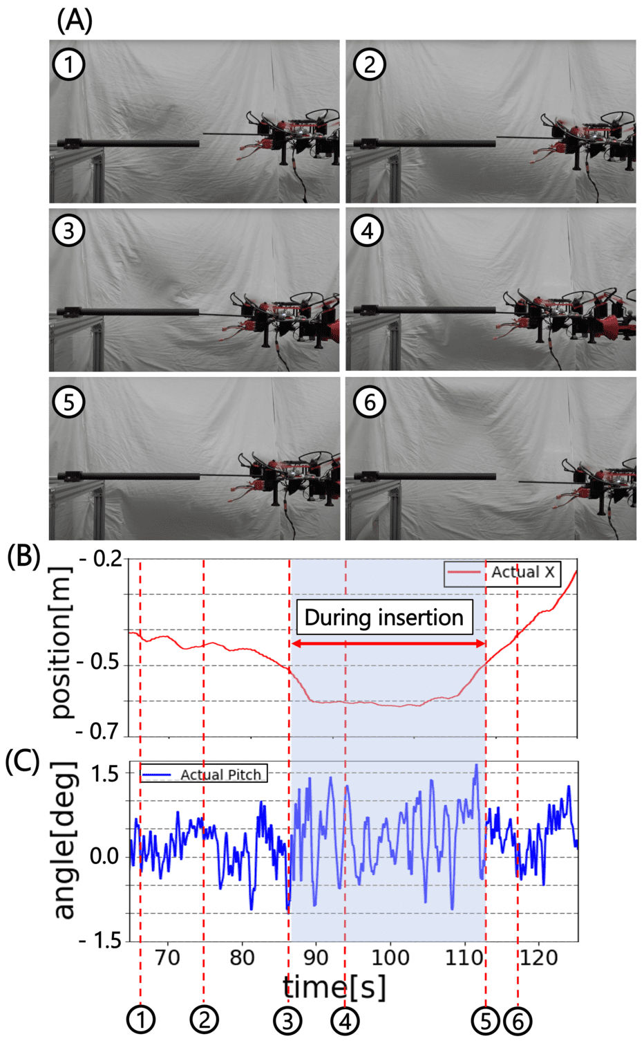
Figure 20: Result of peg insertion experiment. (A)Snapshots of task execution. (B)Plot of the robot position $x$ during the task. (C)Plot of the robot’s pitch angle $\phi$. The sky blue region in the figure is the duration of peg insertion.

VI-E Valve Opening

Finally, to demonstrate the expansion of achievable torque through assembly of units, we conducted a valve opening experiment. An industrial gate valve was used for the experiment, and end effectors for valve operation was attached to the robot. These end effectors are capable of passive expansion and contraction, and do not hinder takeoff and landing. The results of the experiment are presented in Fig. 20. From these results, it was demonstrated that proposed robot TRADY is capable of stable valve opening operations in the air. Fig. 20(B) shows that a maximum torque of $2.4\text{\,}\mathrm{N}\mathrm{m}$ is required during task execution (actually, about $2.2\text{\,}\mathrm{N}\mathrm{m}$ of torque is required to open this valve). Here, it can be seen that by assembling units, the torque performance is improved by approximately nine times with respect to the yaw direction torque that can be exerted in unit state, which is a maximum of $0.28\text{\,}\mathrm{N}\mathrm{m}$. This is due to the fact that the size of the body has increased by assembling units and that torque realization using the horizontal component of rotor thrusts is possible due to the fully-actuated model control.

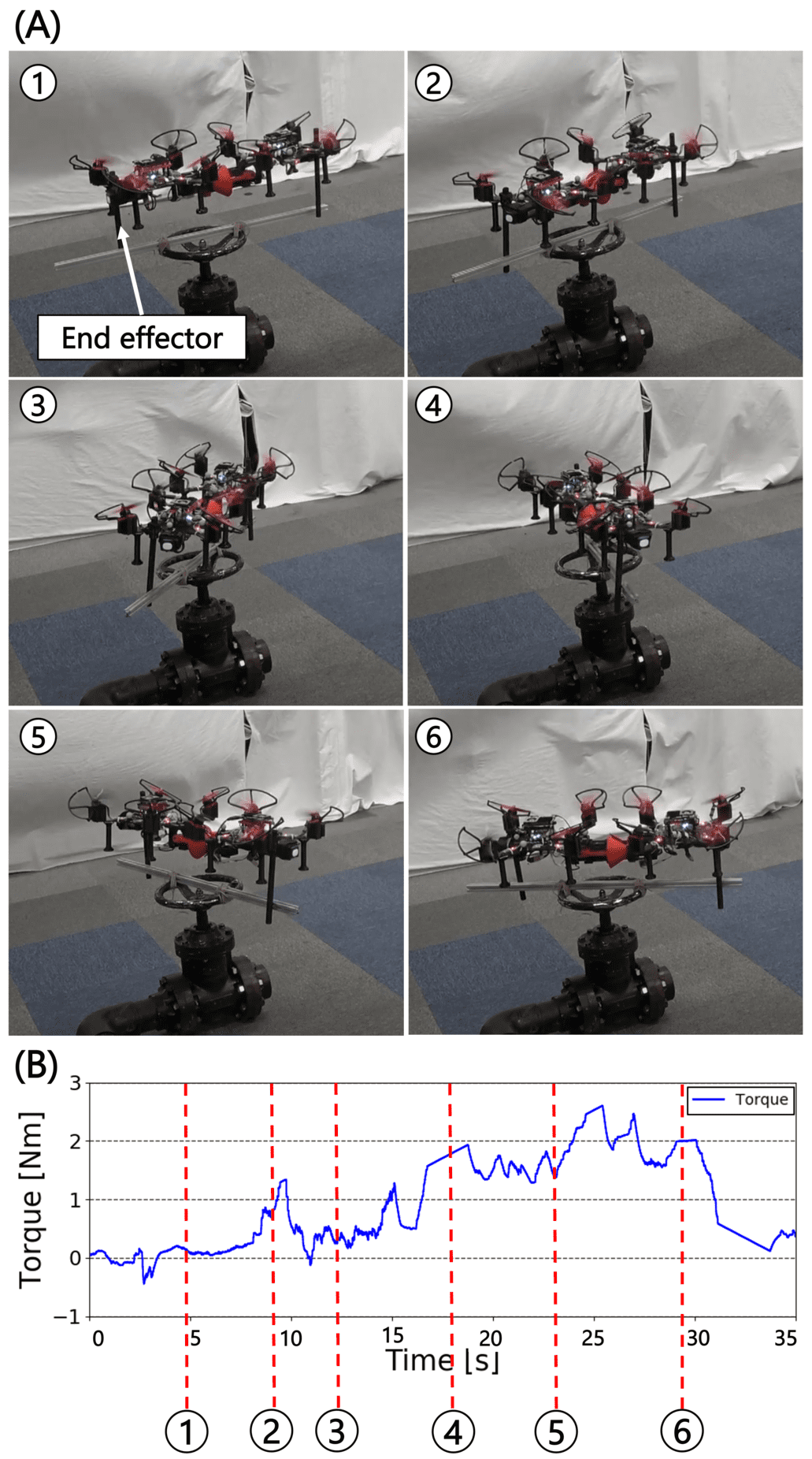
Figure 21: Result of valve opening experiment. (A)Snapshots of task execution. (B)Plot of the robot’s desired torque.

VII Conclusion

In this study, we have developed the configuration of the quadrotor unit named TRADY that possesses the ability to engage in aerial self-assembly and self-disassembly. A noteworthy achievement of this work is that the robot can perform both assembly and disassembly while seamlessly transitioning between fully-actuated and under-actuated models. Building upon the proposed design, control methodology, and motion strategy, we conducted empirical experiments that demonstrated the robot’s ability to perform stable assembly/disassembly movements, as well as execute various aerial manipulation tasks. During the assembly/disassembly experiment, we established that the proposed robot can successfully complete assembly/disassembly movements at a rate of 90%, while also observing that the proposed thrust transition method can suppress instability during switching. Additionally, in the task execution experiment, we determined that the robot in the assembly state can exercise independent control over translation and rotation, while also generating nine times the torque compared to the unitary state.

The pivotal concern that remains in this study is that TRADY, while in the assembly state, is fully-actuated but not omni-directional, which restricts its ability to hover at a significantly tilted posture. As a future prospect, we intend to design a new docking mechanism equipped with joints that will enable the robot to alter rotor directions after assembly. This will expand the robot’s controllability in a more significant manner. Furthermore, expanding the system by utilizing three or more units remains a future challenge. In cases involving three or more units, multiple combinations are possible, allowing for the selection of appropriate units based on the task at hand.

References

- [1] D. Floreano and R. J. Wood, “Science, technology and the future of small autonomous drones,” Nature, vol. 521, pp. 460–466, 2015.
- [2] V. Kumar and N. Michael, “Opportunities and challenges with autonomous micro aerial vehicles,” The International Journal of Robotics Research, vol. 31, no. 11, pp. 1279–1291, 2012.
- [3] R. Bonatti, Y. Zhang, S. Choudhury, W. Wang, and S. Scherer, “Autonomous drone cinematographer: Using artistic principles to create smooth, safe, occlusion-free trajectories for aerial filming,” in Proceedings of the 2018 international symposium on experimental robotics. Springer, 2020, pp. 119–129.
- [4] F. Chataigner, “Arsi: an aerial robot for sewer inspection.” Advances in Robotics Research: From Lab to Market. Springer, Cham, 2020, pp. 249–274, 2020.
- [5] N. Michael, S. Shen, K. Mohta, Y. Mulgaonkar, V. Kumar, K. Nagatani, Y. Okada, S. Kiribayashi, K. Otake, K. Yoshida, K. Ohno, E. Takeuchi, and S. Tadokoro, “Collaborative mapping of an earthquake-damaged building via ground and aerial robots,” Journal of Field Robotics, vol. 29, no. 5, pp. 832–841, 2012.
- [6] L. Doitsidis, S. Weiss, A. Renzaglia, M. W. Achtelik, E. Kosmatopoulos, R. Siegwart, and D. Scaramuzza, “Optimal surveillance coverage for teams of micro aerial vehicles in gps-denied environments using onboard vision,” Autonomous Robots, vol. 33, pp. 173–188, 2012.
- [7] Y. Bai and S. Gururajan, “Evaluation of a baseline controller for autonomous “figure-8” flights of a morphing geometry quadcopter: Flight performance,” Drones, 2019.
- [8] D. Falanga, K. Kleber, S. Mintchev, D. Floreano, and D. Scaramuzza, “The foldable drone: A morphing quadrotor that can squeeze and fly,” IEEE Robotics and Automation Letters, vol. 4, no. 2, pp. 209–216, 2019.
- [9] D. Yang, S. Mishra, D. M. Aukes, and W. Zhang, “Design, planning, and control of an origami-inspired foldable quadrotor,” in 2019 American Control Conference (ACC), 2019, pp. 2551–2556.
- [10] N. Zhao, Y. Luo, H. Deng, and Y. Shen, “The deformable quad-rotor: Design, kinematics and dynamics characterization, and flight performance validation,” in 2017 IEEE/RSJ International Conference on Intelligent Robots and Systems (IROS), 2017, pp. 2391–2396.
- [11] N. Bucki, J. Tang, and M. W. Mueller, “Design and control of a midair-reconfigurable quadcopter using unactuated hinges,” IEEE Transactions on Robotics, vol. 39, no. 1, pp. 539–557, 2023.
- [12] “The voliro omniorientational hexacopter: An agile and maneuverable tiltable-rotor aerial vehicle,” IEEE Robotics and Automation Magazine, vol. 25, pp. 34–44, 12 2018.
- [13] H. B. Khamseh, F. Janabi-Sharifi, and A. Abdessameud, “Aerial manipulation―a literature survey,” Robotics and Autonomous Systems, vol. 107, pp. 221–235, 2018.
- [14] D. Mellinger, Q. Lindsey, M. Shomin, and V. Kumar, “Design, modeling, estimation and control for aerial grasping and manipulation,” in 2011 IEEE/RSJ International Conference on Intelligent Robots and Systems, 2011, pp. 2668–2673.
- [15] G. Heredia, A. Jimenez-Cano, I. Sanchez, D. Llorente, V. Vega, J. Braga, J. Acosta, and A. Ollero, “Control of a multirotor outdoor aerial manipulator,” in 2014 IEEE/RSJ International Conference on Intelligent Robots and Systems, 2014, pp. 3417–3422.
- [16] M. Zhao, K. Kawasaki, K. Okada, and M. Inaba, “Transformable multirotor with two-dimensional multilinks: modeling, control, and motion planning for aerial transformation,” Advanced Robotics, vol. 30, no. 13, pp. 825–845, 2016.
- [17] M. Zhao, F. Shi, T. Anzai, K. Okada, and M. Inaba, “Online motion planning for deforming maneuvering and manipulation by multilinked aerial robot based on differential kinematics,” IEEE Robotics and Automation Letters, vol. 5, no. 2, pp. 1602–1609, 2020.
- [18] H. Yang, S. Park, J. Lee, J. Ahn, D. Son, and D. Lee, “Lasdra: Large-size aerial skeleton system with distributed rotor actuation,” in 2018 IEEE International Conference on Robotics and Automation (ICRA), 2018, pp. 7017–7023.
- [19] M. Zhao, K. Okada, and M. Inaba, “Versatile articulated aerial robot dragon: Aerial manipulation and grasping by vectorable thrust control,” International Journal of Robotics Research, 2022.
- [20] R. Naldi, F. Forte, A. Serrani, and L. Marconi, “Modeling and control of a class of modular aerial robots combining under actuated and fully actuated behavior,” IEEE Transactions on Control Systems Technology, vol. 23, no. 5, pp. 1869–1885, 2015.
- [21] K. Garanger, J. Epps, and E. Feron, “Modeling and experimental validation of a fractal tetrahedron uas assembly,” in 2020 IEEE Aerospace Conference, 2020, pp. 1–11.
- [22] J. Xu, D. S. D’Antonio, and D. Saldana, “H-modquad: Modular multi-rotors with 4, 5, and 6 controllable dof,” vol. 2021-May. Institute of Electrical and Electronics Engineers Inc., 2021, pp. 190–196.
- [23] R. Oung, A. Ramezani, and R. D’Andrea, “Feasibility of a distributed flight array,” in Proceedings of the 48h IEEE Conference on Decision and Control (CDC) held jointly with 2009 28th Chinese Control Conference, 2009, pp. 3038–3044.
- [24] R. Oung, F. Bourgault, M. Donovan, and R. D’Andrea, “The distributed flight array,” in 2010 IEEE International Conference on Robotics and Automation, 2010, pp. 601–607.
- [25] D. Saldana, B. Gabrich, G. Li, M. Yim, and V. Kumar, “Modquad: The flying modular structure that self-assembles in midair.” Institute of Electrical and Electronics Engineers Inc., 9 2018, pp. 691–698.
- [26] D. Saldana, P. M. Gupta, and V. Kumar, “Design and control of aerial modules for inflight self-disassembly,” IEEE Robotics and Automation Letters, vol. 4, pp. 3402–3409, 10 2019.
- [27] I. O’Hara, J. Paulos, J. Davey, N. Eckenstein, N. Doshi, T. Tosun, J. Greco, J. Seo, M. Turpin, V. Kumar, and M. Yim, “Self-assembly of a swarm of autonomous boats into floating structures,” in 2014 IEEE International Conference on Robotics and Automation (ICRA), 2014, pp. 1234–1240.
- [28] K. Yanagimura, K. Ohno, Y. Okada, E. Takeuchi, and S. Tadokoro, “Hovering of mav by using magnetic adhesion and winch mechanisms,” in 2014 IEEE International Conference on Robotics and Automation (ICRA), 2014, pp. 6250–6257.
- [29] M. Ryll, D. Bicego, and A. Franchi, “Modeling and control of fast-hex: A fully-actuated by synchronized-tilting hexarotor,” in 2016 IEEE/RSJ International Conference on Intelligent Robots and Systems (IROS). IEEE, 2016, pp. 1689–1694.
- [30] S. Park, J. Her, J. Kim, and D. Lee, “Design, modeling and control of omni-directional aerial robot,” vol. 2016-November. Institute of Electrical and Electronics Engineers Inc., 11 2016, pp. 1570–1575.
- [31] M. D. Tandale, R. Bowers, and J. Valasek, “Trajectory tracking controller for vision-based probe and drogue autonomous aerial refueling,” Journal of Guidance, Control, and Dynamics, vol. 29, no. 4, pp. 846–857, 2006.
- [32] M. L. Fravolini, A. Ficola, G. Campa, M. R. Napolitano, and B. Seanor, “Modeling and control issues for autonomous aerial refueling for uavs using a probeâdrogue refueling system,” Aerospace Science and Technology, vol. 8, no. 7, pp. 611–618, 2004. [Online]. Available: https://www.sciencedirect.com/science/article/pii/S1270963804000744
- [33] M. Zhao, T. Anzai, K. Okada, K. Kawasaki, and M. Inaba, “Singularity-free aerial deformation by two-dimensional multilinked aerial robot with 1-dof p vectorable propeller,” IEEE Robotics and Automation Letters, vol. 6, pp. 1367–1374, 4 2021.
- [34] P. Bosscher, A. Riechel, and I. Ebert-Uphoff, “Wrench-feasible workspace generation for cable-driven robots,” IEEE Transactions on Robotics, vol. 22, no. 5, pp. 890–902, 2006.
- [35] N. Documentation, “Nlopt algorithms,” https://nlopt.readthedocs.io/en/latest/NLopt_Algorithms/#isres-improved-stochastic-ranking-evolution-strategy.
- [36] T. Lee, M. Leok, and N. H. McClamroch, “Geometric tracking control of a quadrotor uav on se(3),” in 49th IEEE Conference on Decision and Control (CDC), 2010, pp. 5420–5425.
- [37] P. Young and J. Willems, “An approach to the linear multivariable servomechanism problem,” International Journal of Control, vol. 15, 06 1972.