Topological dynamical quantum phase transition in a quantum skyrmion phase

Abstract

Quantum skyrmionic phase is modelled in a 2D helical spin lattice. This topological skyrmionic phase retains its nature in a large parameter space before moving to a ferromagnetic phase. Next nearest-neighbour interaction improves the stability and it also causes a shift of the topological phase in the parameter space. Nonanalytic behaviour of the rate function observed, when the system which is initially in a quantum skyrmion phase is quenched to a trivial quantum ferromagnetic phase, indicates a dynamical quantum phase transition. Dynamical quantum phase transition is absent when the system initially in a skyrmion phase is quenched to a helical phase.

Progresses made in the last decade in controlling matter at quantum levels allow access to real-time dynamics of closed quantum many-body systems realisable Bloch et al. (2008, 2012). This progress lifted the border between experimentally feasible physical reality and model systems. Ultra-cold atoms in optical lattices and trapped ions are examples in which such dynamical phenomena were observed in real-time. Nowadays, we have full access to the real-time dynamics of quantum many-body and finite systems, either isolated or coupled to the Markovian or non-Markovian environment. The experiments with THz pulses in solids Cole et al. (2001); Huber et al. (2001); Kaindl et al. (2003); Iwai et al. (2003), high magnetic field pulse experiments Weickert et al. (2012)etc. are also developments in recent past which can be aided by theoretical understanding of dynamical properties of the corresponding quantum systems especially the study of the evolution of the system after a sudden change in its parameter or a quantum quench. When we talk about changing the parameter of a system, the first thing that pops up in our mind is the term phase transition. Phase transitions are the points in the parameter space of a system around which a small change in the control parameter manifests a drastic change to its characteristics. In a classical/thermal phase transition, the thermal fluctuations cause the destruction of long-range ordering and facilitate the phase transition. But when we study the changes of the parameters at zero temperature or ground states the characteristics of the phase transition become purely quantum, because here the phase transition is facilitated by quantum fluctuations instead of thermal fluctuations. Such phase transitions are known as quantum phase transitions. Equilibrium quantum phase transitions(EQPT) are studied extensively but we have a lesser understanding of quantum systems out of equilibrium. In order to theoretically aid the experimental developments mentioned earlier we need to understand the dynamical quantum phase transitions(DQPT). Recent experimental developments identified a signature of dynamical behaviour after a quench in a Haldane-like system Fläschner et al. (2018). Experiments with trapped ions were able to directly observe DQPTs Jurcevic et al. (2017). The theoretical inspiration for the DQPT can be extracted from Lee-Yang theorem, Fisher zero’s and accompanying analysis. (For more details refer to Zvyagin (2016))

From Lee-Yang analysis Yang and Lee (1952); Lee and Yang (1952) one can arrive at the conclusion that for a partition function of external fields (like magnetic field), which also depended on the temperature $T$ as $Z(T)$, when zeros exist and have a positive real value then each of those roots corresponds to nonanalyticity in the free energy, i.e., phase transition. Fisher extended this analysis considering partition functions with complex temperature $z$ instead of $T$, $Z(z)$. When Fisher’s zeros of $Z(z)$ overlap with the real axis it produces nonanalyticities or phase transitions, however, no such overlaps is observed in the course of an EQPT. The real values of Fisher’s zeros correspond to a different kind of phase transition, namely DQPT Zvyagin (2016); Heyl (2018). Using these analyses essence of DQPTs can be explained briefly as follows Heyl et al. (2013); Deger et al. (2020); Vosk and Altman (2014); Gulácsi et al. (2020):

Short-lived non-equilibrium phase transitions accompanied with a nonanalytic behaviour of physical quantities as a function of time is a characteristic feature of DQPTs Heyl et al. (2013). To study this we utilise a quantity $\mathcal{G}$ the Loschmidt amplitude as a function of time $t$, given as

$$\mathcal{G}(t)=\langle\psi_{0}|e^{-i\hat{H}t}|\psi_{0}\rangle.$$ (1)

In a sense, it plays the same role in the study of states out-of-equilibrium as the partition function $Z=Tr(e^{-\beta\hat{H}})$ in thermodynamic equilibrium case. Here $\hat{H}$ is the Hamiltonian of the system and $\beta$ is the inverse temperature and $\psi_{0}$ is the initial state of the system. Here $Z$ can be seen as the kind of partition function considered by Lee and Yang(with inverse temperature in place of temperature, still the conclusions of the analysis holds). And in the exponent term of $\mathcal{G}(t)$ if we take $(it)$ as the complex temperature, $\mathcal{G}$ behaves like partition function of complex temperature considered by Fisher.

Another quantity of interest is the rate function of the return probability, Eq. 2 (hereinafter referred to as rate function) which is analogous to the thermodynamic free energy. As discussed earlier during a phase transition the thermodynamic free energy, $F=-\frac{ln(Z)}{\beta}$, turns out to be a nonanalytic function of a control parameter. Based on the analogy we established so far, we expect to see a nonanalytic behaviour on $\mathcal{L}$ when there is a DQPT, since it is a dynamical analogue of thermodynamic free energy. The rate function is given as:

$$\mathcal{L}(t)=-\lim_{N\rightarrow\infty}\frac{1}{N}\ln|\mathcal{G}(t)|^{2},$$ (2)

where $N$ is the number of degrees of freedom of the system.

DQPT is intensively studied during the last decade Heyl (2018); Kyaw et al. (2020); Jafari and Akbari (2021); Azimi et al. (2016); Masłowski and Sedlmayr (2020); Langen et al. (2015). In the present work we are interested in the interplay between topology and DQPTs considering the quantum skyrmion Sotnikov et al. (2021). The scientific community is still fascinated about topological states of matter even though it has been over four decades since the discovery of the Quantum Hall state, the first discovered topological state Prange and Girvin (1987). Topologically distinct states or topological states are those states, which are classified based on a certain invariant Altland and Simons (2010); Zeng et al. (2019). Such states are said to be identical when we can move from one state to another by applying continuous smooth deformations(deformations which do not close the bulk energy gap) without changing the value of the invariant Qi and Zhang (2011). When the system shows this kind of resistance to deformation we say that it is topologically protected. Conventional states, which are earlier believed to be the same may become topologically distinct. We discover this only when the accompanying physical behaviour is detected, like in the case of the Quantum Hall effect.

In the past few decades, scientists discovered many topological materials and states like topological insulators Haldane (1988); König et al. (2007), topological crystaline insulators Hsieh et al. (2012); Tanaka et al. (2012), topological semi-metals Fu and Kane (2007); Schindler et al. (2018) etc. This classification is based on the behaviour of the corresponding band Hamiltonians in the reciprocal state. There are also nontrivial topological objects determined by their characteristics in real space such as various types of topological defects in condensed matter Mermin (1979).

Magnetic skyrmions are among the most popular types of topological defects studied now. Skyrmions are particular examples of solitons that can be informally defined as localized waves with a stable shape (for more accurate definition and detailed discussion see e.g. Rajaraman (1982a)). They are related to peculiar localized non-colinear magnetic textures within magnetic systems Piette et al. (1995); Rajaraman (1982b); Skyrme (1994). Skyrmions are promised to be potential information carriers for the next generation of spintronic devices Bogdanov and Panagopoulos (2020). New studies suggest macroscopic skyrmion qubits design suitable for quantum computing technology controlling the helicity and dynamics of the skyrmions through electric fields Psaroudaki and Panagopoulos (2021). These developments make the study of the dynamics of quantum skyrmions demanding.

The formation of magnetic order in spin systems depends on different factors and competing interactions. Formation of non-colinear magnetic textures is mainly fueled either by competing nearest-neighbor ferromagnetic and next nearest-neighbor antiferromagnetic or asymmetric exchange interactions termed as Dzyaloshinskii–Moriya interaction (DMI). In most cases, the DMI is the dominant mechanism forming non-conventional magnetic textures Belavin and Polyakov (1975); Barton-Singer et al. (2020); Schroers (1995); Seki et al. (2012); Wilson et al. (2014); Schütte and Garst (2014); White et al. (2014); Derras-Chouk et al. (2018a); Haldar et al. (2018); Leonov and Mostovoy (2015); Psaroudaki et al. (2017); van Hoogdalem et al. (2013); Rohart et al. (2016); Samoilenka and Shnir (2017); Battye and Haberichter (2013); Jennings and Winyard (2014); Tsesses et al. (2018).

Recently, the quantum analog of magnetic skyrmions has been suggested and studied Lohani et al. (2019); Gauyacq and Lorente (2019); Sotnikov et al. (2021). However, contrary to the classical skyrmion the quantum skyrmion is not topologically stable in a rigorous sense. Qualitatively, it is not protected with respect to the quantum tunneling to the topologically trivial vacuum state. At the same time, it presents a quantum spin state with quite a special character reminiscent of its topologically protected classical analog. Here we use the words "topological phase" for the case of quantum skyrmions in this, not completely rigorous but intuitively clear, sense. To better understand the nature of this state we studied its real-time dynamical properties.

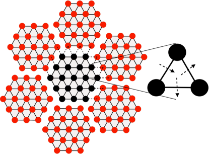
Figure 1: PBC is applied to the 19 spins central super-cell(black unit of the lattice). Super cell is repeated due to the PBC such that it forms a larger triangular lattice. The solid bonds show bonds within the boundary and the dashed bonds represent PBC. The bonds of this lattice can be classified into three based on their orientation. Hence the direction of corresponding DMI vectors is also different for each one of these categories of bonds. Three types of bonds and direction of corresponding DMI vectors(dashed arrows) can be seen in the figure inset.

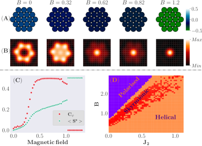
Figure 2: (A) Locations of spins and spin textures of the local magnetization of a system at different values of an applied magnetic field. Here $D=1,\>J_{1}=-0.5D,\>J_{2}=0.1D$. The colors quantify expectation values of $\hat{S}_{z}$ components of specific spins. (B) The Fourier transform of the longitudinal spin correlation function for $D=1,\>J_{1}=-0.5D,\>J_{2}=0.1D$. The observed intensity peaks confirm the formation of non-trivial magnetic textures. (C) For $D=1,\>J_{1}=-0.5D,\>J_{2}=0.1D$, the quantum scalar chirality remains constant between magnetic field values of $0.46D$ and $0.86D$. (D) A phase diagram showing ferromagnetic, skyrmionic and helical phases using the scalar chirality in the $J_{2}-B$ parametric space.

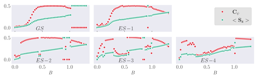
Figure 3: Chirality and magnetization vs field for first few eigen states for $D=1,\>J_{1}=-0.5D,\>J_{2}=0.1D$. Here in the panel GS stands for the ground state, and ES stands for exited states. In GS, ES-1, ES-2, and ES-3, we can identify the scalar chirality $C_{\psi}$ with the almost constant value (at $C_{\psi}\sim 0.5$) corresponding to a certain range of the magnetic field $B$. For the GS the range of $B$ is $B\sim 0.48D$ to $B\sim 0.91D$. In ES-1 it is $B\sim 0.48D$ to $B\sim 0.89D$. In ES-2 it is $B\sim 0.48D$ to $B\sim 0.85D$. In ES-3 it is $B\sim 0.59D$ to $B\sim 0.79D$. We notice that for higher excited energy levels the range of the plateau is diminished, and at ES-4 we completely lost the plateau. An important fact is that already for the first excited state ES-1, we observe fluctuation in the case of the strong field $B\sim 0.9D$. For higher excited states ES-2 and ES-3 fluctuations are enhanced and features of the quantum skyrmion state are absent.

Unlike skyrmions, Ochoa and Tserkovnyak (2019); Derras-Chouk et al. (2018b); Stepanov et al. (2019); Lohani et al. (2019); Wang et al. (2020) helical magnetic textures do not possess a topological invariant and a topological protection. Any classification of 2D helical phases is difficult, even properties of quantum skyrmions are not well explored. Recent attempts to discover quantum skyrmions show a certain degree of success. Lohani et.al. Lohani et al. (2019) and Gauyacq et.al. Gauyacq and Lorente (2019) could identify magnetization patterns of a quantum skyrmion but topological protection of skyrmion phase was not explored. Sotnikov et.al. used a quantum scalar chirality to identify a topological protectionSotnikov et al. (2021). Siegl et.al. using topological index and winding parameters, were able to identify a skyrmion phase and quantify its stability Siegl et al. (2022). All these works could only find a skyrmionic phase in the ground state. In the present work, we investigate the stability of quantum skyrmions in higher excited levels as well.

An important question is the strength of the DM interaction. DMI can be determined in experiments or calculated accurately from first-principles Fert et al. (2017); Yang et al. (2023). Our interest is focused on materials with large DMI: Li et al. (2022); Liang et al. (2020); Zhang et al. (2020). In recent experimental works H. Yang et.al Zhang et al. (2018) has shown that magnetic films sandwiched between nonmagnetic layers exhibit DMI with an electrically tunable strength, i.e., Co films sandwiched between nonmagnetic layers or MgO/Fe/Pt. The value of DMI in such materials linearly increases with the applied external electric field $D=D_{0}+g_{ME}E$, where $D_{0}$ is the intrinsic DMI part, $g_{ME}$ is the magnetoelectric coupling and $E$ is the external electric field. Enhanced DMI can formally reach the order of exchange interaction for a large electric field. The dynamic control of intrinsic magnetic interactions by varying the strength of a high-frequency laser field allows further enhancing of the ratio between DMI and exchange interaction constants Stepanov et al. (2019, 2017); Itin and Katsnelson (2015); Schüler et al. (2013). The idea relies on the fact that DMI and exchange interaction are both based on hopping processes and that time-periodic fields renormalize the electronic tunneling, leading to the effective rescaled DMI and exchange constants $D\approx\frac{4t\Delta}{U_{0}-U}$ and $J\approx\frac{4t^{2}}{\Omega^{2}}(U_{0}-U)$. Here $\Delta$ describes the Rashba spin-orbit coupling, $t$ denotes the hopping amplitude, $U_{0}-U$ is the gain in the Coulomb energy due to the electron displacement, and $\Omega$ is the frequency of the laser field. Because of the factor $1/\Omega^{2}$, the high-frequency laser field can substantially reduce the rescaled exchange constant to achieve the condition $D>J$. In order to study Helical-Skyrmionic-Ferromagnetic phases we consider an array of spins formed in a triangular lattice. The spins are arranged in such a way that it has a six-fold rotation symmetry (see Fig. 1), also with periodic boundary conditions (PBC) it possesses translation symmetry. The Hamiltonian of the system has the form:

$$\hat{H}=B\sum\limits_{i}\hat{\mathbf{S}_{i}^{z}}+J_{1}\sum\limits_{\langle i,j\rangle}\hat{\mathbf{S}_{i}}\hat{\mathbf{S}_{j}}+ J_{2}\sum\limits_{\langle{\langle i,j\rangle}\rangle}\hat{\mathbf{S}_{i}}\hat{\mathbf{S}_{j}}$$

$$+\sum\limits_{i<j}\textbf{D}_{i,j}\left[\hat{\mathbf{S}_{i}}\times\hat{\mathbf{S}_{j}}\right],$$ (3)

where summation in single brackets is taken over the nearest neighbors and in double brackets over the next-nearest-neighbors, $B$ is an external magnetic field, and the DMI vector D is aligned perpendicular to the bond between lattice sites $i$ and $j$, see inset of Fig. (1). The direction of DMI vectors is chosen to ensure that the six-fold rotation symmetry holds. We note that in helical multiferroic insulators, the parameter $D$ is an effect of the magnetoelectric coupling $g_{ME}$ with an external electric field $E$, i.e., $D=g_{ME}E$. Thus, the strength of the DMI term can be controlled externally Wang et al. (2020). Here we consider both $J_{1}$(a ferromagnetic nearest neighbor exchange) and $J_{2}$ (an anti-ferromagnetic next nearest neighbor exchange) interactions along with the DMI.

An array of spins read along with the above Hamiltonian with a specific parameter set forms a quantum skyrmion. The nearest-neighbor ferromagnetic $J_{1}$ term encourages colinear spin orientation while DMI term compels non-colinear spin texture. These two competing interactions form classical skyrmions stabilized by the applied magnetic field. Below we show that adding even small next nearest neighbor antiferromagnetic Heisenberg term $J_{2}$ improves the stability of quantum skyrmion structures. In general, it is well-known that the $J_{2}$ term leads to the spin frustration and formation of antiferromagnetic classical skyrmions Okubo et al. (2012) However, quantum skyrmion structures are quite specific as compared to classical skyrmions. In particular, quantum skyrmions do not possess continuous magnetic texture and topological charge. Therefore to infer the quantum skyrmion state, we exploit another tool, such as scalar chirality. The energy levels of the system Eq.(Topological dynamical quantum phase transition in a quantum skyrmion phase) show a six-fold degeneracy even at very high magnetic field values. We calculated the expectation values considering maximally mixed state of these degenerate states with equal probability.

We used spin correlation functions to characterise quantum non-trivial magnetic structures. In particular, we explore the Fourier transform of the longitudinal spin correlation function $G_{\|}(\textbf{q})=\dfrac{1}{N}\sum\limits_{ij}G_{\|}(\textbf{r}_{ij})\exp(-i\textbf{q}\textbf{r}_{ij})$, where $N$ is the number of spins and the correlation function is given by

$$G_{\|}(\textbf{r}_{ij})=\frac{1}{Z}\sum\limits_{n}\langle n|\hat{S}_{i}^{z}\hat{S}_{j}^{z}|n\rangle\exp(-\beta E_{n}).$$ (4)

where $E_{n}$s are the eigenvalues of the Hamiltonian of the system and $r_{ij}$ is the distance between the lattice sites $i$ and $j$.

Topologically protected systems like skyrmions tend to show resistance to a deformation in its configurationJe et al. (2020); Braun (2012). Throughout this work an applied magnetic field is considered as a cause of deformation. In Fig. 2(A) and Fig. 2(B) panels are arranged in the increasing order of applied magnetic field from left to right. Fig. 2(A) shows that the local magnetisation is uniform and increasing magnetic field causes the local magnetisation to increase in the direction of the field. This observation fails to identify any magnetic textures in the system. Fig. 2(B), multiple intensity spots (Bragg peaks) observed for nonzero q(Fourier conjugate of $r$ or wave vector in reciprocal space) confirms formation of the quantum non-trivial magnetic texture Stepanov et al. (2019). This quantity could distinguish between helical and ferromagnetic phases but it fails to identify skyrmionic phase within the helical phase. So we require another quantifier that can trace out the skyrmion phase from helical and ferromagnetic phases.

Scalar chirality Sotnikov et al. (2021)

$$\textbf{C}_{\Psi}=\frac{\mathcal{N}}{\pi}\left\langle\hat{S}_{1}\left[\hat{S}_{2}\times\hat{S}_{3}\right]\right\rangle.$$ (5)

is considered as a distinguishing property of a helical spin system. When the chirality has a non-zero value we say that the system is in a helical phase. It is proposed that chirality can distinguish quantum skyrmion phase from other phases of the system Sotnikov et al. (2021).

In this equation $\mathcal{N}$ is the number of non-overlapping elementary triangular patches covering the lattice. Three adjacent spins form a patch. The scalar chirality for any of these three adjacent spin combinations is the same, because of the translational and rotational symmetries of the lattice.

In Fig. 2(C) from $B=0D$ to $B=0.46D$ chirality increases almost steadily. In this region no two deformed states have same chirality value, therefore, all those states are topologically non-identical. From $B=0.46D$ till $B=0.86D$ the plateau of scalar chirality implies that all the states in this region have a common topological invariant and we call them topologically identical phase or simply topological phase. After crossing $B=0.86D$ the system briefly falls back to a helical phase. It is represented by a dip in chirality. Then around $B=1.0D$ the system goes to the trivial ferromagnetic phase indicated by zeros of scalar chirality.

In Fig. 2(C) The magnetisation graph is telling us that for the region where we have plateau in chirality the magnetisation is not same for any two states i.e., the system is in fact undergoing deformation during the constant chirality plateau also.

The phase diagram (Fig. 2(D)) shows that for non zero $J_{2}$ the invariance of scalar chirality extends for larger values of the applied magnetic field compared to $J_{2}=0$. The skyrmion phase is embedded into the helical phase. For a larger value of the interaction parameter $J_{2}$, the system retains the skyrmion phase for a longer range of applied magnetic field. We studied the scalar chirality not only in the ground state but also in several excited states. We see that the skyrmion state survives in first and second excited states as well as a certain degree of topological invariance can be seen in higher excited states, see Fig. 3. When $J_{2}=0D$ we arrive at the results from O. M. Sotnikov et. al. Sotnikov et al. (2021). For higher values of $J_{2}$($J_{2}>0.35D$) the plateau gets distorted.

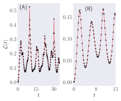
Figure 4: Quench protocol is applied on ground state initiated with $D=1$, $J_{1}=-0.5D$, $J_{2}=0.1D$, $B=0.85D$. (A) Time evolution of rate function for skyrmionic to polar phase transition. At $t=0$ DMI is turned off (set $D=0$). The peak of rate function at $t=9.71,\>30.1\>etc.\$ shows nonanalytic behaviour. (B) Time evolution of rate function for skyrmionic to Helical phase transition. At $t=0$ the applied field, $B$ is turned off. Here we do not find any nonanalyticity.

Here we show that an important information about helical and quantum skyrmion phases can be obtained from the analyses of topological DQPTs. Namely, when quenching the system from a quantum skyrmion to a topologically trivial phase, we observe a characteristic signature of a DQPT as a nonanalyticity in the rate function. On the other hand, a quench between a skyrmion and a helix does not lead to a DQPT.

Let the system be prepared in the ground state $|\psi_{0}\rangle$ of the Hamiltonian $\hat{H}_{0}=\hat{H}(\lambda_{0})$. At $t=0$ the parameter $\lambda$ is quenched to a new value $\hat{H}(\lambda_{f})$ and the initial wave function is evolved to a new state $|\psi(t)\rangle=e^{-i\hat{H}t}|\psi_{0}\rangle$ under this new Hamiltonian. In order to describe the DQPT we study the Loschmidt amplitude (return amplitude) and the rate function, in the thermodynamic limit Heyl (2014); Brandner et al. (2017); Lang et al. (2018); Tian et al. (2020); Nie et al. (2020); Pastori et al. (2020).

Our primary interest concerns DQPTs between a quantum skyrmion phase and a trivial phase. The quench protocol applied on a topological phase to a trivial (skyrmion to ferromagnet) phase produced a nonanalytic behaviour of the rate function with respect to time. The result is plotted in Fig. 4(A). On the other hand, when switching between a skyrmionic phase to a helical phase, we do not observe any DQPT. We can confirm this from the lack of nonanalytic behaviour of the rate function when plotted against time in Fig. 4(B). Here we looked for nonanalyticity with different values of the parameter $B$ but we could not find any. The presence of nonanalyticity in the former case can be explained by a sharp and discontinuous transition of $\boldsymbol{C_{\psi}}$ from skyrmionic to trivial phase in Fig. 2(C). Similarly the lack of nonanalyticity in the later case is due to the smooth and continuous transition of $\boldsymbol{C_{\psi}}$ from helical to skyrmionic phase. From Fig. 4(A) the critical exponent $\alpha=0.7020\pm 0.0233$ around $t_{c}=9.66$. The value turned out to be very close to this for other critical points as well (see supplementary methods for details section I, see, also, references Trapin et al. (2021); Heyl (2015); Bandyopadhyay et al. (2021) therein). Further study is required with larger system sizes($L=3i(i+1)+1,\>i=3,\,4,\,5,\,...$) in order to comment on the universality of the critical exponent that we calculated.

We have computational limitations to analyzing finite-size effects and artifacts of a particular quantum skyrmion state in our system. However, we performed the study of the finite-size effects using another quantum skyrmion state obtained for a slightly different model in Siegl et al. (2022). The results of the calculations are shown in section I. We see the same trend for this case also, i. e., non-analytic singularities in the rate function during the dynamical quantum phase transition between the skyrmion and FM phases. Thus obtained results are pretty universal and apply to any quantum skyrmion. The reason for the universal effect is the orthogonality of quantum skyrmion and FM states. This argument is valid for any quantum skyrmion independently of its size.

Apart from this, we achieved a significant improvement of the topological phase stability with our model compared to the previous works Sotnikov et al. (2021); Lohani et al. (2019); Siegl et al. (2022). We note that within a skyrmionic phase a larger $J_{2}$ value gives a topological phase protection against a larger range of applied magnetic fields. At high values of $J_{2}$ the topological invariance is destroyed. This result tells us that the key for tunability and improved stability of quantum skyrmions can be the interaction parameter, this may be useful when choosing the material to realise skyrmions for experiments. This kind of model is realized in Pd/Fe/Ir(111) system with Co surrounded edges Spethmann et al. (2022). Also nanoscale skyrmions are reported at room temperature with large DMI interaction in Ir/CoFeB/MgO systems Chen et al. (2021).

In conclusion, the quantum skyrmion model proposed above shows significant improvement in topological protection. In the said model we identified a robust DQPT when quench protocol is applied from a skyrmionic state to a ferromagnetic state. Robust DQPTs accompany many interesting properties. An interesting direction is to look for the connection between entanglement dynamics and DQPTs in a skyrmionic phase. Certain systems have reported to show an enhanced entanglement entropy around critical points of DQPTs Jurcevic et al. (2017).

I Supplemental material to “Topological dynamical quantum phase transition in a quantum skyrmion phase"

Calculation of critical exponent $\mathbf{\alpha}$

We adopted a method discussed by Trapin et al Trapin et al. (2021) to calculate the critical exponent of DQPT. For a one dimensional system Trapin et al report $\alpha=0.1264(2)$ which is less than the value defined by universality class of the problem. They call it as an unconventional critical exponent.

It is a well known fact that the critical exponents depend on factors like dimension of the system, range of the interaction and spin dimension.

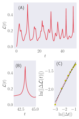
Figure 5: How to calculate critical exponent associated to a nonanalyticity. (A) Rate function showing nonanalyticity. (B) Zoomed in on the first nonanalytic point at $t\sim 43.24$. (C) $\ln(|\Delta\mathcal{L}|)$ vs. $\ln(|\Delta t|)$: Red line with green dots is observed data, black dashed line is the straight line approximation.

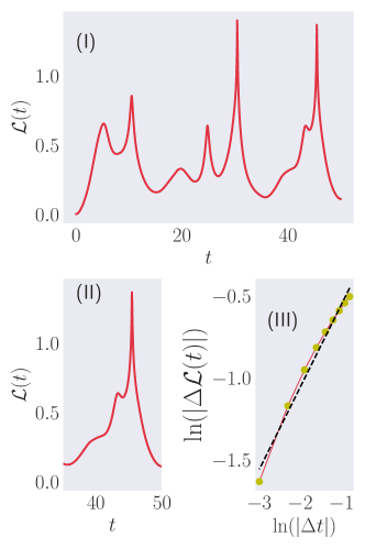
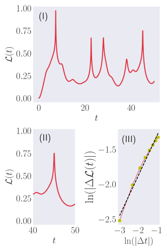
(A)	(B)

Figure 6: (A) Critical exponent in DQPT of a $3\times 3$ square lattice. (I) Rate function showing nonanalyticity. (II) Zoomed in on a nonanalytic point at $t\sim 45.44$. (III) $\ln(|\Delta\mathcal{L}|)$ vs. $\ln(|\Delta t|)$: Red line with green dots is observed data, black dashed line is the straight line approximation. (B) Critical exponent in DQPT of a $4\times 4$ square lattice. (I) Rate function showing nonanalyticity. (II) Zoomed in on a nonanalytic point at $t\sim 45$. (III) $\ln(|\Delta\mathcal{L}|)$ vs. $\ln(|\Delta t|)$: Red line with green dots is observed data, black dashed line is the straight line approximation.

Contrary to the system we have in this manuscript, Trapin et al only consider a one dimensional chain with nearest-neighbour interaction, this can cause a difference in the value of $\alpha$ that we calculate. Attempts were made to find universality and scaling for DQPTs for one and two dimensional systems Heyl (2015). For 1d system the exponent $\alpha$ is reported to be 1. A recent work by Bandyopadhyay et al. Bandyopadhyay et al. (2021) outlines a protocol based on out of time order correlations(OTOC) and string-like observables to experimentally determine the critical exponents of DQPT. Using the method they show a universal scaling critical exponent for one dimensional systems to be $\alpha=1$. But for 2D systems the analysis in Heyl (2015) could not find a conclusive value for $\alpha$ in general.Nonetheless we may still calculate $\alpha$ for our system using the method discussed by Trapin et al.. Let $t-t_{c}$ denote a nonanalytic point. We can approximate the rate function $\mathcal{L}(t)$ around the nonanalyticity as follows,

$$|\mathcal{L}(t)-\mathcal{L}_{c}|\sim|t-t_{c}|^{\alpha}.$$ (6)

Taking logarithm on both sides of Eq. (6) gives us the equation of a straight line with slope $\alpha$.

Consider $\Delta t=t-t_{c}$ and $\Delta\mathcal{L}=\mathcal{L}(t)-\mathcal{L}_{c}$. We plot $\ln(|\Delta\mathcal{L}|)$ versus $\ln(|\Delta t|)$ and fit it to a straight line that best fits. The slope of the straight line is the exponent $\alpha$. Let us consider the nonanalytic point in Fig. 5(A) which is around $t_{c}=43.24$. This region is highlighted in Fig. 5(B). Now if we plot $\ln(|\Delta\mathcal{L}|)$ versus $\ln(|\Delta t|)$ and fit a straight line as shown in Fig. 5(C), the exponent $\alpha$ at $t_{c}=43.24$ is determined to be $0.4883\pm 0.0218$ with this method. The critical exponent $\alpha$ turned out to be similar for other $t_{c}$ values as well, e. g., $\alpha=0.7020\pm 0.0233$ for $t_{c}=9.66$.

Since we have computational limitations in our model to look for different system sizes, to accommodate for the finite size effect we consider the skyrmion model proposed by Siegl et.al Siegl et al. (2022).

Consider an $n\times n$ lattice of quantum spin-1/2’s coupled to classical ferromagnetic control fields at its boundary. The Hamiltonian of the system is given as,

$$\hat{H}= -J\sum\limits_{\langle i,j\rangle}(S_{i}^{x}S_{j}^{x}+S_{i}^{y}S_{j}^{y})-\Delta\sum\limits_{\langle i,j\rangle}S_{i}^{z}S_{j}^{z}$$ (7)

$$-D\sum\limits_{\langle i,j\rangle}(\mathbf{u_{ij}}\times\hat{z}).\left(\mathbf{S}_{i}\times\mathbf{S}_{j}\right),$$

with ferromagnetic exchange constant $J>0$, axial Heisenberg anisotropy $\Delta>0$, and the strength of DMI interaction $D$. $\mathbf{u_{ij}}$ is a vector pointing from $\mathbf{S_{i}}$ to $\mathbf{S_{j}}$. $\mathbf{\hat{S}_{i}}=(S_{i}^{x},S_{i}^{y},S_{i}^{z})$ is a vector of spin operators for spins within the $n\times n$ lattice. A layer of classical ferromagnetic spins $S_{i}=\frac{\hbar}{2}\hat{z}$ resides outside the lattice.

Further in order to define a skyrmion we utilize the following quantities.

$$\begin{rcases}Q\\ C\end{rcases}=\frac{1}{2\pi}\sum\limits_{\sigma}\tan^{-1}\left(\frac{\mathbf{n}_{i}(\mathbf{n}_{j}\times\mathbf{n}_{k})}{1+\mathbf{n}_{i}\mathbf{n}_{j}+\mathbf{n}_{i}\mathbf{n}_{k}\mathbf{n}_{k}\mathbf{n}_{j}}\right),$$ (8)

where the sum runs over all the elementary triangles formed by nearest-neighbour lattice sites $i,$ $j$, $k$ which include the classical ferromagnetic boundary sites as well and no two triangles overlap. The magnitude of the winding parameter $Q$ quantifies the stability of the skyrmion. It is computed with $\mathbf{n_{i}}=2\langle\mathbf{S}_{i}\rangle\hbar$, where $\langle\mathbf{S}_{i}\rangle=(\langle S_{i}^{x}\rangle,\langle S_{i}^{y}\rangle,\langle S_{i}^{z}\rangle)$ is the classical magnetic moment or spin expectation value. The topological index $C$ takes $\mathbf{n_{i}}=\langle\mathbf{S}_{i}\rangle/|\langle\mathbf{S}_{i}\rangle|$. $C=\pm 1$ for quantum skyrmions.

For a $3\times 3$ lattice when $\Delta=0.5J$ and $D=2J$ we identified a quantum skyrmion phase with $C=-1$ and $Q=-0.981$. We note that parameters $\Delta=0.5J$ and $D=0$ give a quantum ferromagnet with $C=0$ and $Q=0$. Fig.  6(A) shows the rate function and the calculation of critical exponent for this case. The critical exponent in this case is calculated to be $0.5020\pm 0.0240$. Similar observations were done with $4\times 4$ lattice case also, where parameters $\Delta=0.5J$ and $D=2J$ get a skyrmion phase with $C=-1$ and $Q=-0.981$. $D=0$ gives a ferromagnetic ground state with $C=0$ and $Q=0$. We initiate the system from the skyrmion phase and at $t=0$ we quench the system by setting $D=0$. The results are summarised in Fig.  6(B). The critical exponent in this case is found to be $0.5667\pm 0.02878$.

Next, we investigate DQPT on another 2d model considering a triangular lattice within a circle with ferromagnetic classical boundaries having the following Hamiltonian,

$$\hat{H}= -J_{1}\sum\limits_{\langle i,j\rangle}(S_{i}^{x}S_{j}^{x}+S_{i}^{y}S_{j}^{y})-K\sum\limits_{\langle i,j\rangle}S_{i}^{z}S_{j}^{z}$$ (9)

$$+\mathbf{D_{1}}\sum\limits_{\langle i,j\rangle}\left(\mathbf{S}_{i}\times\mathbf{S}_{j}\right),$$

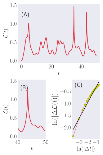
Figure 7: Nonanalytic rate function and the calculation of exponent for a 7-spin triangular lattice. (A) Rate function is showing nonanalyticity. (B) Zoomed in on nonanalytic point at $t\sim 43.58$. (C) $\ln(|\Delta\mathcal{L}|)$ vs. $\ln(|\Delta t|)$: Red line with green dots is observed data, black dashed line is the straight line approximation.

Here $J_{1}>0$ is the nearest-neighbour ferromagnetic coupling constant, $K>0$ is the axial Heisenberg anisotropy coefficient and $D_{1}>0$ is the strength of the DMI vector $\mathbf{D_{1}}$. The direction of DMI is the same as the one shown in Fig. 1 . $\mathbf{\hat{S}_{i}}=(S_{i}^{x},S_{i}^{y},S_{i}^{z})$ is a vector of spin operators for spins within the circular triangular lattice. A layer of classical ferromagnetic spins $S_{i}=\frac{\hbar}{2}\hat{z}$ resides outside the lattice. We make use of the quantities $Q$ and $C$ to identify quantum skyrmions here also.

In a 7-spin triangular lattice case with circular boundary for $J_{1}=1$, $K=0.61J_{1}$ and $D_{1}=2J_{1}$ we see a skyrmion phase with $C=1$ and $Q=0.993$. In the same configuration $D_{1}=0$ gives a ferromagnetic phase with $C=0$ and $Q=0$. We initiated the system at the skyrmion phase and quenched it to a ferromagnetic phase by setting $D_{1}=0$ at $t=0$. The resulting rate function is shown in Fig.  7. The critical exponent calculated is $0.6130\pm 0.0191$ at $t_{c}=43.58$.

We observed DQPT in various systems with different geometry and interactions around the same time domain $43.24<t_{c}<45.44$ with system sizes 7, 9, 16, 19 and the critical exponents for respective sizes are $0.6130\pm 0.0191$, $0.5020\pm 0.0240$, $0.5667\pm 0.02878$ and $0.4883\pm 0.0218$. This is shown in Fig.  8. In the all cases we find the exponents around 0.5, which hints a universality in skyrmion to ferromagnetic state DQPT.

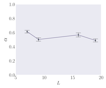
Figure 8: Critical exponents $\alpha$ in DQPT of three similar 2d models vs. system size $L$ around the same time domain $43.24<t_{c}<45.44$. All the cases show a universal exponent around $0.5$.

References

- Bloch et al. (2008) I. Bloch, J. Dalibard, and W. Zwerger, Reviews of Modern Physics 80, 885 (2008), arXiv:0704.3011 [cond-mat.other] .
- Bloch et al. (2012) I. Bloch, J. Dalibard, and S. Nascimbène, Nature Physics 8, 267 (2012).
- Cole et al. (2001) B. Cole, J. Williams, B. King, M. Sherwin, and C. Stanley, Nature 410, 60—63 (2001).
- Huber et al. (2001) R. Huber, F. Tauser, A. Brodschelm, M. Bichler, G. Abstreiter, and A. Leitenstorfer, Nature 414, 286 (2001).
- Kaindl et al. (2003) R. A. Kaindl, M. A. Carnahan, D. Hägele, R. Lövenich, and D. S. Chemla, Nature 423, 734 (2003).
- Iwai et al. (2003) S. Iwai, M. Ono, A. Maeda, H. Matsuzaki, H. Kishida, H. Okamoto, and Y. Tokura, Phys. Rev. Lett. 91, 057401 (2003).
- Weickert et al. (2012) F. Weickert, B. Meier, S. Zherlitsyn, T. Herrmannsdörfer, R. Daou, M. Nicklas, J. Haase, F. Steglich, and J. Wosnitza, Measurement Science and Technology 23, 105001 (2012).
- Fläschner et al. (2018) N. Fläschner, D. Vogel, M. Tarnowski, B. S. Rem, D. S. Lühmann, M. Heyl, J. C. Budich, L. Mathey, K. Sengstock, and C. Weitenberg, Nature Physics 14, 265 (2018).
- Jurcevic et al. (2017) P. Jurcevic, H. Shen, P. Hauke, C. Maier, T. Brydges, C. Hempel, B. P. Lanyon, M. Heyl, R. Blatt, and C. F. Roos, Phys. Rev. Lett. 119, 080501 (2017).
- Zvyagin (2016) A. Zvyagin, Low Temperature Physics 42, 971 (2016).
- Yang and Lee (1952) C. N. Yang and T. D. Lee, Phys. Rev. 87, 404 (1952).
- Lee and Yang (1952) T. D. Lee and C. N. Yang, Phys. Rev. 87, 410 (1952).
- Heyl (2018) M. Heyl, Reports on Progress in Physics 81, 054001 (2018).
- Heyl et al. (2013) M. Heyl, A. Polkovnikov, and S. Kehrein, Phys. Rev. Lett. 110, 135704 (2013).
- Deger et al. (2020) A. Deger, F. Brange, and C. Flindt, Phys. Rev. B 102, 174418 (2020).
- Vosk and Altman (2014) R. Vosk and E. Altman, Phys. Rev. Lett. 112, 217204 (2014).
- Gulácsi et al. (2020) B. Gulácsi, M. Heyl, and B. Dóra, Phys. Rev. B 101, 205135 (2020), arXiv:2002.10296 [cond-mat.quant-gas] .
- Kyaw et al. (2020) T. H. Kyaw, V. M. Bastidas, J. Tangpanitanon, G. Romero, and L.-C. Kwek, Physical Review A 101, 012111 (2020).
- Jafari and Akbari (2021) R. Jafari and A. Akbari, Phys. Rev. A 103, 012204 (2021).
- Azimi et al. (2016) M. Azimi, M. Sekania, S. K. Mishra, L. Chotorlishvili, Z. Toklikishvili, and J. Berakdar, Phys. Rev. B 94, 064423 (2016).
- Masłowski and Sedlmayr (2020) T. Masłowski and N. Sedlmayr, Phys. Rev. B 101, 014301 (2020).
- Langen et al. (2015) T. Langen, R. Geiger, and J. Schmiedmayer, Annual Review of Condensed Matter Physics 6, 201 (2015), arXiv:1408.6377 [cond-mat.quant-gas] .
- Sotnikov et al. (2021) O. M. Sotnikov, V. V. Mazurenko, J. Colbois, F. Mila, M. I. Katsnelson, and E. A. Stepanov, Phys. Rev. B 103, L060404 (2021).
- Prange and Girvin (1987) R. E. Prange and S. M. Girvin, The Quantum Hall Effect (Springer New York, 1987).
- Altland and Simons (2010) A. Altland and B. D. Simons, Condensed Matter Field Theory, 2nd ed. (Cambridge University Press, 2010).
- Zeng et al. (2019) B. Zeng, X. Chen, D. Zhou, and X. Wen, Quantum Information Meets Quantum Matter: From Quantum Entanglement to Topological Phases of Many-Body Systems, Quantum Science and Technology (Springer New York, 2019).
- Qi and Zhang (2011) X.-L. Qi and S.-C. Zhang, Reviews of Modern Physics 83, 1057 (2011), arXiv:1008.2026 [cond-mat.mes-hall] .
- Haldane (1988) F. D. M. Haldane, Phys. Rev. Lett. 61, 2015 (1988).
- König et al. (2007) M. König, S. Wiedmann, C. Brüne, A. Roth, H. Buhmann, L. W. Molenkamp, X.-L. Qi, and S.-C. Zhang, Science 318, 766 (2007), https://www.science.org/doi/pdf/10.1126/science.1148047 .
- Hsieh et al. (2012) T. H. Hsieh, H. Lin, J. Liu, W. Duan, A. Bansil, and L. Fu, Nature Communications 3, 982 (2012), arXiv:1202.1003 [cond-mat.mtrl-sci] .
- Tanaka et al. (2012) Y. Tanaka, Z. Ren, T. Sato, K. Nakayama, S. Souma, T. Takahashi, K. Segawa, and Y. Ando, Nature Physics 8, 800 (2012), arXiv:1206.5399 [cond-mat.mes-hall] .
- Fu and Kane (2007) L. Fu and C. L. Kane, Phys. Rev. B 76, 045302 (2007).
- Schindler et al. (2018) F. Schindler, Z. Wang, M. G. Vergniory, A. M. Cook, A. Murani, S. Sengupta, A. Y. Kasumov, R. Deblock, S. Jeon, I. Drozdov, H. Bouchiat, S. Guéron, A. Yazdani, B. A. Bernevig, and T. Neupert, Nature Physics 14, 918 (2018), arXiv:1802.02585 [cond-mat.mtrl-sci] .
- Mermin (1979) N. D. Mermin, Rev. Mod. Phys. 51, 591 (1979).
- Rajaraman (1982a) R. Rajaraman, Solitons and Instantons: An Introduction to Solitons and Instantons in Quantum Field Theory, North-Holland personal library (North-Holland Publishing Company, 1982).
- Piette et al. (1995) B. M. Piette, B. J. Schroers, and W. Zakrzewski, Zeitschrift für Physik C Particles and Fields 65, 165 (1995).
- Rajaraman (1982b) R. Rajaraman, in Solitons and instantons: an introduction to solitons and instantons in quantum field theory (North-Holland, 1982).
- Skyrme (1994) T. H. R. Skyrme, in Selected Papers, With Commentary, Of Tony Hilton Royle Skyrme (World Scientific, 1994) pp. 195–206.
- Bogdanov and Panagopoulos (2020) A. N. Bogdanov and C. Panagopoulos, Nature Reviews Physics 2, 492 (2020), arXiv:2008.00641 [cond-mat.mes-hall] .
- Psaroudaki and Panagopoulos (2021) C. Psaroudaki and C. Panagopoulos, Phys. Rev. Lett. 127, 067201 (2021), arXiv:2108.02219 [cond-mat.mes-hall] .
- Belavin and Polyakov (1975) A. Belavin and A. Polyakov, JETP lett 22, 245 (1975).
- Barton-Singer et al. (2020) B. Barton-Singer, C. Ross, and B. J. Schroers, Communications in Mathematical Physics 375, 2259 (2020).
- Schroers (1995) B. J. Schroers, Physics Letters B 356, 291 (1995).
- Seki et al. (2012) S. Seki, X. Yu, S. Ishiwata, and Y. Tokura, Science 336, 198 (2012).
- Wilson et al. (2014) M. Wilson, A. Butenko, A. Bogdanov, and T. Monchesky, Physical Review B 89, 094411 (2014).
- Schütte and Garst (2014) C. Schütte and M. Garst, Physical Review B 90, 094423 (2014).
- White et al. (2014) J. White, K. Prša, P. Huang, A. Omrani, I. Živković, M. Bartkowiak, H. Berger, A. Magrez, J. Gavilano, G. Nagy, et al., Physical review letters 113, 107203 (2014).
- Derras-Chouk et al. (2018a) A. Derras-Chouk, E. M. Chudnovsky, and D. A. Garanin, Physical Review B 98, 024423 (2018a).
- Haldar et al. (2018) S. Haldar, S. von Malottki, S. Meyer, P. F. Bessarab, and S. Heinze, Physical Review B 98, 060413 (2018).
- Leonov and Mostovoy (2015) A. Leonov and M. Mostovoy, Nature communications 6, 1 (2015).
- Psaroudaki et al. (2017) C. Psaroudaki, S. Hoffman, J. Klinovaja, and D. Loss, Physical Review X 7, 041045 (2017).
- van Hoogdalem et al. (2013) K. A. van Hoogdalem, Y. Tserkovnyak, and D. Loss, Physical Review B 87, 024402 (2013).
- Rohart et al. (2016) S. Rohart, J. Miltat, and A. Thiaville, Physical Review B 93, 214412 (2016).
- Samoilenka and Shnir (2017) A. Samoilenka and Y. Shnir, Physical Review D 95, 045002 (2017).
- Battye and Haberichter (2013) R. A. Battye and M. Haberichter, Physical Review D 88, 125016 (2013).
- Jennings and Winyard (2014) P. Jennings and T. Winyard, Journal of High Energy Physics 2014, 122 (2014).
- Tsesses et al. (2018) S. Tsesses, E. Ostrovsky, K. Cohen, B. Gjonaj, N. Lindner, and G. Bartal, Science 361, 993 (2018).
- Lohani et al. (2019) V. Lohani, C. Hickey, J. Masell, and A. Rosch, Phys. Rev. X 9, 041063 (2019).
- Gauyacq and Lorente (2019) J. P. Gauyacq and N. Lorente, Journal of Physics Condensed Matter 31, 335001 (2019), arXiv:1904.03926 [cond-mat.mes-hall] .
- Ochoa and Tserkovnyak (2019) H. Ochoa and Y. Tserkovnyak, International Journal of Modern Physics B 33, 1930005 (2019).
- Derras-Chouk et al. (2018b) A. Derras-Chouk, E. M. Chudnovsky, and D. A. Garanin, Phys. Rev. B 98, 024423 (2018b).
- Stepanov et al. (2019) E. Stepanov, S. Nikolaev, C. Dutreix, M. Katsnelson, and V. Mazurenko, Journal of Physics: Condensed Matter 31, 17LT01 (2019).
- Wang et al. (2020) X.-G. Wang, L. Chotorlishvili, N. Arnold, V. K. Dugaev, I. Maznichenko, J. Barnaś, P. A. Buczek, S. S. P. Parkin, and A. Ernst, Phys. Rev. Lett. 125, 227201 (2020).
- Siegl et al. (2022) P. Siegl, E. Y. Vedmedenko, M. Stier, M. Thorwart, and T. Posske, Phys. Rev. Res. 4, 023111 (2022).
- Fert et al. (2017) A. Fert, N. Reyren, and V. Cros, Nature Reviews Materials 2, 17031 (2017).
- Yang et al. (2023) H. Yang, J. Liang, and Q. Cui, Nature Reviews Physics 5, 43 (2023).
- Li et al. (2022) P. Li, Q. Cui, Y. Ga, J. Liang, and H. Yang, Phys. Rev. B 106, 024419 (2022).
- Liang et al. (2020) J. Liang, W. Wang, H. Du, A. Hallal, K. Garcia, M. Chshiev, A. Fert, and H. Yang, Phys. Rev. B 101, 184401 (2020).
- Zhang et al. (2020) Y. Zhang, C. Xu, P. Chen, Y. Nahas, S. Prokhorenko, and L. Bellaiche, Phys. Rev. B 102, 241107 (2020).
- Zhang et al. (2018) W. Zhang, H. Zhong, R. Zang, Y. Zhang, S. Yu, G. Han, G. L. Liu, S. S. Yan, S. Kang, and L. M. Mei, Applied Physics Letters 113, 122406 (2018), https://doi.org/10.1063/1.5050447 .
- Stepanov et al. (2017) E. A. Stepanov, C. Dutreix, and M. I. Katsnelson, Phys. Rev. Lett. 118, 157201 (2017).
- Itin and Katsnelson (2015) A. P. Itin and M. I. Katsnelson, Phys. Rev. Lett. 115, 075301 (2015).
- Schüler et al. (2013) M. Schüler, M. Rösner, T. O. Wehling, A. I. Lichtenstein, and M. I. Katsnelson, Phys. Rev. Lett. 111, 036601 (2013).
- Okubo et al. (2012) T. Okubo, S. Chung, and H. Kawamura, Phys. Rev. Lett. 108, 017206 (2012).
- Je et al. (2020) S.-G. Je, H.-S. Han, S. K. Kim, S. A. Montoya, W. Chao, I.-S. Hong, E. E. Fullerton, K.-S. Lee, K.-J. Lee, M.-Y. Im, and et al., ACS Nano 14, 3251–3258 (2020).
- Braun (2012) H.-B. Braun, Advances in Physics 61, 1 (2012), https://doi.org/10.1080/00018732.2012.663070 .
- Heyl (2014) M. Heyl, Phys. Rev. Lett. 113, 205701 (2014).
- Brandner et al. (2017) K. Brandner, V. F. Maisi, J. P. Pekola, J. P. Garrahan, and C. Flindt, Phys. Rev. Lett. 118, 180601 (2017).
- Lang et al. (2018) J. Lang, B. Frank, and J. C. Halimeh, Phys. Rev. Lett. 121, 130603 (2018).
- Tian et al. (2020) T. Tian, H.-X. Yang, L.-Y. Qiu, H.-Y. Liang, Y.-B. Yang, Y. Xu, and L.-M. Duan, Phys. Rev. Lett. 124, 043001 (2020).
- Nie et al. (2020) X. Nie, B.-B. Wei, X. Chen, Z. Zhang, X. Zhao, C. Qiu, Y. Tian, Y. Ji, T. Xin, D. Lu, and J. Li, Phys. Rev. Lett. 124, 250601 (2020).
- Pastori et al. (2020) L. Pastori, S. Barbarino, and J. C. Budich, Phys. Rev. Research 2, 033259 (2020).
- Trapin et al. (2021) D. Trapin, J. C. Halimeh, and M. Heyl, Phys. Rev. B 104, 115159 (2021).
- Heyl (2015) M. Heyl, Phys. Rev. Lett. 115, 140602 (2015).
- Bandyopadhyay et al. (2021) S. Bandyopadhyay, A. Polkovnikov, and A. Dutta, Phys. Rev. Lett. 126, 200602 (2021).
- Spethmann et al. (2022) J. Spethmann, E. Y. Vedmedenko, R. Wiesendanger, A. Kubetzka, and K. von Bergmann, Communications Physics 5, 19 (2022).
- Chen et al. (2021) R. Chen, X. Wang, H. Cheng, K.-J. Lee, D. Xiong, J.-Y. Kim, S. Li, H. Yang, H. Zhang, K. Cao, M. Kläui, S. Peng, X. Zhang, and W. Zhao, Cell Reports Physical Science 2, 100618 (2021).