Pixel-wise Gradient Uncertainty for Convolutional Neural Networks applied to Out-of-Distribution Segmentation

Abstract

In recent years, deep neural networks have defined the state-of-the-art in semantic segmentation where their predictions are constrained to a predefined set of semantic classes. They are to be deployed in applications such as automated driving, although their categorically confined expressive power runs contrary to such open world scenarios. Thus, the detection and segmentation of objects from outside their predefined semantic space, i.e., out-of-distribution (OoD) objects, is of highest interest. Since uncertainty estimation methods like softmax entropy or Bayesian models are sensitive to erroneous predictions, these methods are a natural baseline for OoD detection. Here, we present a method for obtaining uncertainty scores from pixel-wise loss gradients which can be computed efficiently during inference. Our approach is simple to implement for a large class of models, does not require any additional training or auxiliary data and can be readily used on pre-trained segmentation models. Our experiments show the ability of our method to identify wrong pixel classifications and to estimate prediction quality at negligible computational overhead. In particular, we observe superior performance in terms of OoD segmentation to comparable baselines on the SegmentMeIfYouCan benchmark, clearly outperforming other methods.

1 INTRODUCTION

Semantic segmentation decomposes the pixels of an input image into segments which are assigned to a fixed and predefined set of semantic classes. In recent years, deep neural networks (DNNs) have performed excellently in this task [Chen et al., 2018, Wang et al., 2021], providing comprehensive and precise information about the given scene. However, in safety-relevant applications like automated driving where semantic segmentation is used in open world scenarios, DNNs often fail to function properly on unseen objects for which the network has not been trained, see for example the bobby car in Figure 1 (top). These objects from outside the network’s semantic space are called out-of-distribution (OoD) objects.

Figure 1: Top: Semantic segmentation by a deep neural network. Bottom: Gradient uncertainty heatmap obtained by our method.

It is of highest interest that the DNN identifies such objects and abstains from deciding on the semantic class for those pixels covered by the OoD object. Another case are OoD objects which might belong to a known class, however, appearing differently to substantial significance from other objects of the same class seen during training. Consequently, the respective predictions are prone to error. For these objects, as for classical OoD objects, marking them as OoD is preferable to the likely case of misclassification which may happen with high confidence. This additional classification task should not substantially degrade the semantic segmentation performance itself outside the OoD region. The computer vision tasks of identifying and segmenting those objects is called OoD segmentation [Chan et al., 2021a, Maag et al., 2022].

The recent contributions to the emerging field of OoD segmentation are mostly focused on OoD training, i.e., the incorporation of additional training data (not necessarily from the real world), sometimes obtained by large reconstruction models [Biase et al., 2021, Lis et al., 2019]. Another line of research is the use of uncertainty quantification methods such as Bayesian models [Mukhoti and Gal, 2018] or maximum softmax probability [Hendrycks and Gimpel, 2016]. Gradient-based uncertainties are considered for OoD detection in the classification task [Huang et al., 2021, Lee et al., 2022, Oberdiek et al., 2018] but up to now, have not been applied to OoD segmentation. In [Grathwohl et al., 2020], it is shown that gradient norms perform well in discriminating between in- and out-of-distribution. Moreover, gradient-based features are studied for object detection to estimate the prediction quality in [Riedlinger et al., 2023]. In [Hornauer and Belagiannis, 2022], loss gradients w.r.t. feature activations in monocular depth estimation are investigated and show correlations of gradient magnitude with depth estimation accuracy.

In this work, we introduce a new method for uncertainty quantification in semantic segmentation based on gradient information. Magnitude features of gradients can be computed at inference time and provide information about the uncertainty propagated in the corresponding forward pass. The features represent pixel-wise uncertainty scores applicable to prediction quality estimation and OoD segmentation. An exemplary gradient uncertainty heatmap can be found in Figure 1 (bottom). Calculating gradient uncertainty scores does not require any re-training of the DNN or computationally expensive sampling. Instead, only one backpropagation step for the gradients with respect to the final convolutional network layer is performed per inference to produce gradient scores. Note, that more than one backpropagation step can be performed to compute deeper gradients which considers other parameters of the model architecture. An overview of our approach is shown in Figure 2.

An application to dense predictions such as semantic segmentation has escaped previous research, potentially due to the superficial computational overhead. Single backpropagation steps per pixel on high-resolution input images quickly become infeasible given that around $10^{6}$ gradients have to be calculated. To overcome this issue, we present a new approach to exactly compute the pixel-wise gradient scores in a batched and parallel manner applicable to a large class of segmentation architectures. This is possible due to a convenient factorization of $p$-norms for appropriately factorizing tensors, such as the gradients for convolutional neural networks. We use the computed gradient scores to estimate the model uncertainty on pixel-level and also the prediction quality on segment-level. Moreover, the gradient uncertainty heatmaps are investigated for OoD segmentation where high scores indicate possible OoD objects. We demonstrate the efficiency of our method in explicit runtime measurements and show that the computational overhead introduced is marginal compared with the forward pass. This suggests that our method is applicable in extremely runtime-restricted applications of semantic segmentation.

For our method, we only assume a pre-trained semantic segmentation network ending on a convolutional layer which is a common case. In our experiments, we employ a state-of-the-art semantic segmentation network [Chen et al., 2018] trained on Cityscapes [Cordts et al., 2016] evaluating in-distribution uncertainty estimation. We demonstrate OoD detection performance on four well-known OoD segmentation datasets, namely LostAndFound [Pinggera et al., 2016], Fishyscapes [Blum et al., 2019a], RoadAnomaly21 and RoadObstacle21 [Chan et al., 2021a]. The source code of our method is made publicly available at https://github.com/tobiasriedlinger/uncertainty-gradients-seg. We summarize our contributions as follows:

• We introduce a new gradient-based method for uncertainty quantification in semantic segmentation. This approach is applicable to a wide range of common segmentation architectures.

• For the first time, we show an efficient way of computing gradient norms in semantic segmentation on the pixel-level in a parallel manner making our method far more efficient than sampling-based methods which is demonstrated in explicit time measurements.

• We demonstrate the effectiveness of our method to predictive error detection and OoD segmentation. For OoD segmentation, we achieve area under precision-recall curve values of up to $69.3\%$ on the LostAndFound benchmark outperforming a variety of methods.

2 RELATED WORK

Uncertainty Quantification.

Bayesian approaches [MacKay, 1992] are widely used to estimate model uncertainty. The well-known approximation, MC Dropout [Gal and Ghahramani, 2016], has proven to be computationally feasible for computer vision tasks and has also been applied to semantic segmentation [Lee et al., 2020]. In addition, this method is considered to filter out predictions with low reliability [Wickstrøm et al., 2019]. In [Blum et al., 2019a], pixel-wise uncertainty estimation methods are benchmarked based on Bayesian models or the network’s softmax output. Uncertainty information is extracted on pixel-level by using the maximum softmax probability and MC Dropout in [Hoebel et al., 2020]. Prediction quality evaluation approaches were introduced in [DeVries and Taylor, 2018, Huang et al., 2016] and work on single objects per image. These methods are based on additional CNNs acting as post-processing mechanism. The concepts of meta classification (false positive / FP detection) and meta regression (performance estimation) on segment-level were introduced in [Rottmann et al., 2020]. This line of research has been extended by a temporal component [Maag et al., 2020] and transferred to object detection [Schubert et al., 2021, Riedlinger et al., 2023] as well as to instance segmentation [Maag et al., 2021, Maag, 2021].

While MC Dropout as a sampling approach is still computationally expensive to create pixel-wise uncertainties, our method computes only the gradients of the last layer during a single inference run and can be applied to a wide range of semantic segmentation networks without architectural changes. Compared with the work presented in [Rottmann et al., 2020], our gradient information can extend the features extracted from the segmentation network’s softmax output to enhance the segment-wise quality estimation.

OoD Segmentation.

Uncertainty quantification methods demonstrate high uncertainty for erroneous predictions, so they are often applied to OoD detection. For instance, this can be accomplished via maximum softmax (probability) [Hendrycks and Gimpel, 2016], MC Dropout [Mukhoti and Gal, 2018] or deep ensembles [Lakshminarayanan et al., 2017] the latter of which also capture model uncertainty by averaging predictions over multiple sets of parameters in a Bayesian manner. Another line of research is OoD detection training, relying on the exploitation of additional training data, not necessarily from the real world, but disjoint from the original training data [Blum et al., 2019b, Chan et al., 2021b, Grcic et al., 2022, Grcic et al., 2023, Liu et al., 2023, Nayal et al., 2023, Rai et al., 2023, Tian et al., 2022]. In this regard, an external reconstruction model followed by a discrepancy network is considered in [Biase et al., 2021, Lis et al., 2019, Lis et al., 2020, Vojir et al., 2021, Vojíř and Matas, 2023] and normalizing flows are leveraged in [Blum et al., 2019b, Grcic et al., 2021, Gudovskiy et al., 2023]. In [Lee et al., 2018, Liang et al., 2018], adversarial perturbations are performed on the input images to improve the separation of in- and out-of-distribution samples.

Specialized training approaches for OoD detection are based on different kinds of re-training with additional data and often require generative models. Meanwhile, our method does not require OoD data, re-training or complex auxiliary models. Moreover, we do not run a full backward pass which is, however, required for the computation of adversarial samples. In fact we found that it is often sufficient to only compute the gradients of the last convolutional layer. Our method is more related to classical uncertainty quantification approaches like maximum softmax, MC Dropout and ensembles. Note that the latter two are based on sampling and thus, much more computationally expensive compared to single inference.

3 METHOD DESCRIPTION

In the following, we consider a neural network with parameters $\theta$ yielding classification probabilities $\hat{\pi}(x,\theta)=(\hat{\pi}_{1},\ldots,\hat{\pi}_{C})$ over $C$ semantic categories when presented with an input $x$. During training on paired data $(x,y)$, where $y\in\{1,\ldots,C\}$ is the semantic label given to $x$, such a model is commonly trained by minimizing some kind of loss function $\mathcal{L}$ between $y$ and the predicted probability distribution $\hat{\pi}(x,\theta)$ using gradient descent on $\theta$. The gradient step $\nabla_{\!\theta}\mathcal{L}(\hat{\pi}(x,\theta)\|y)$ then indicates the direction and strength of training feedback obtained by $(x,y)$. Asymptotically (in the amount of data and training steps taken), the expectation $\mathbb{E}_{(X,Y)\sim P}[\nabla_{\!\theta}\mathcal{L}(\hat{\pi}(X,\theta)\|Y)]$ of the gradient w.r.t. the data generating distribution $P$ will vanish since $\theta$ sits at a local minimum of $\mathcal{L}$. We assume, that strong models which achieve high test accuracy can be seen as an approximation of such a parameter configuration $\theta$. Such a model has small gradients on in-distribution data which is close to samples $(x,y)$ in the training data. Samples that differ from training data may receive larger feedback. Like-wise, it is plausible to obtain large training gradients from OoD samples that are far away from the effective support of $P$.

In order to quantify uncertainty about the prediction $\hat{\pi}(x,\theta)$, we replace the label $y$ from above by some fixed auxiliary label for which we make two concrete choices in our method. On the one hand, we replace $y$ by the class prediction one-hot vector $y^{\mathit{oh}}_{k}=\delta_{k\hat{c}}$ with $\hat{c}=\mathrm{arg\,max}_{k=1,\ldots,C}\,\hat{\pi}_{k}$ and the Kronecker symbol $\delta_{ij}$. This quantity correlates strongly with training labels $y$ on in-distribution data. On the other hand, we regard a constant uniform, all-warm label $y^{\mathit{uni}}_{k}=1/C$ for $k=1,\ldots,C$ as a replacement for $y$. To motivate the latter choice, we consider that classification models are oftentimes trained on the categorical cross entropy loss

$$\mathcal{L}(\hat{\pi}\|y)=-\sum_{k=1}^{C}y_{k}\log(\hat{\pi}_{k}).$$ (1)

Since the gradient of this loss function is linear in the label $y$, a uniform choice $y^{\mathit{uni}}$ will return the average gradient per class which is expected to be large on OoD data where all possible labels are similarly unlikely. The magnitude of $\nabla_{\!\theta}\mathcal{L}(\hat{\pi}\|y)$ serves as uncertainty / OoD score. In the following, we explain how to compute such scores for pixel-wise classification models.

3.1 Efficient Computation in Semantic Segmentation

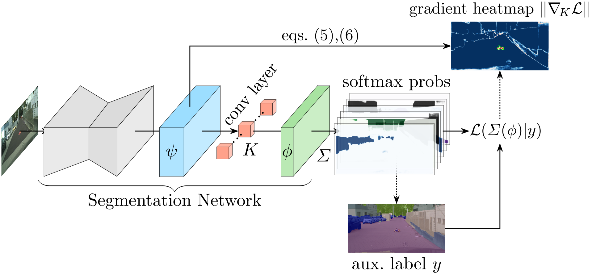
Figure 2: Schematic illustration of the computation of pixel-wise gradient norms for a semantic segmentation network with a final convolution layer. Auxiliary labels may be derived from the softmax prediction or supplied in any other way (e.g., as a uniform all-warm label). We circumvent direct back propagation per pixel by utilizing eqs. (5), (6).

We regard a generic segmentation architecture utilizing a final convolution as the pixel-wise classification mechanism. In the following, we also assume that the segmentation model is trained via the commonly-used pixel-wise cross entropy loss $\mathcal{L}_{ab}(\phi(\theta)|y)$ (cf. eq. (1)) over each pixel $(a,b)$ with feature map activations $\phi(\theta)$. However, similarly compact formulas hold for arbitrary loss functions. Pixel-wise probabilities are obtained by applying the softmax function $\varSigma$ to each output pixel, i.e., $\hat{\pi}_{ab,k}=\varSigma^{k}\left(\phi_{ab}(\theta)\right)$. With eq. (1), we find for the loss gradient

$$\nabla_{\!\theta}\mathcal{L}_{ab}(\varSigma(\phi(\theta))\|y)=\sum_{k=1}^{C}\varSigma^{k}(\phi_{ab})(1-y_{k})\cdot\nabla_{\!\theta}\phi^{k}_{ab}(\theta).$$ (2)

Here, $\theta$ is any set of parameters within the neural network. Detailed derivations of this and the following formulas of this section are provided in Appendix A. Here, $\phi$ is the convolution result of a pre-convolution feature map $\psi$ (see Figure 2) against a filter bank $K$ which assumes the role of $\theta$. $K$ has parameters $(K_{e}^{h})_{fg}$ where $e$ and $h$ indicate in- and out-going channels respectively and $f$ and $g$ index the spatial filter position. The features $\phi$ are linear in both, $K$ and $\psi$, and explicitly depend on bias parameters $\beta$ in the form

$$\phi_{ab}^{d}=(K\ast\psi)_{ab}^{d}+\beta^{d}=\sum_{j=1}^{\kappa}\sum_{p,q=-s}^{s}(K_{j}^{d})_{pq}\psi^{j}_{a+p,b+q}+\beta^{d}.$$ (3)

We denote by $\kappa$ the total number of in-going channels and $s$ is the spatial extent to either side of the filter $K_{j}^{d}$ which has total size $(2s+1)\times(2s+1)$. We make different indices in the convolution explicit in order to compute the exact gradients w.r.t. the filter weights $(K_{e}^{h})_{fg}$, where we find for the last layer gradients

$$\frac{\partial\phi_{ab}^{d}}{\partial(K_{e}^{h})_{fg}}=\delta_{dh}\psi_{a+f,b+g}^{e}.$$ (4)

Together with eq. (2), we obtain the closed form for computing the correct backpropagation gradients of the loss on pixel-level for our choices of auxiliary labels which we state in the following paragraph. The computation of the loss gradient can be traced in Figure 2.

If we take the predicted class $\hat{c}$ as a one-hot label per pixel as auxiliary labels, i.e., $y^{\mathit{oh}}$, we obtain for the last layer gradients

$$\frac{\partial\mathcal{L}_{ab}(\varSigma(\phi)\|y^{\mathit{oh}})}{\partial K_{e}^{h}}=\varSigma^{h}(\phi_{ab})\cdot(1-\delta_{h\hat{c}})\cdot\psi_{ab}^{e}$$ (5)

which depends on quantities that are easily accessible during a forward pass through the network. Note, that the filter bank $K$ for the special case of ($1\times 1$)-convolutions does not require spatial indices which is a common situation in segmentation networks, albeit, not necessary for our method to be applied. Similarly, we find for the uniform label $y^{\mathit{uni}}_{j}=1/C$

$$\frac{\partial\mathcal{L}_{ab}(\varSigma(\phi)\|y^{\mathit{uni}})}{\partial K_{e}^{h}}=\frac{C-1}{C}\varSigma^{h}(\phi_{ab})\psi_{ab}^{e}.$$ (6)

These formulas reveal a practical factorization of the gradient which we will exploit computationally in the next section. Therefore, pixel-wise gradient norms are simple to implement and particularly efficient to compute for the last layer of the segmentation model. In Appendix A.2, we cover formulas for the more general case of deeper gradients, as well.

3.2 Uncertainty Scores

We obtain pixel-wise scores, i.e., still depending on $a$ and $b$, by computing the partial norm $\|\nabla_{\!K}\mathcal{L}_{ab}\|_{p}$ of this tensor over the indices $e$ and $h$ for some fixed value of $p$. This can again be done in a memory efficient way by the natural decomposition $\partial\mathcal{L}/\partial K_{e}^{h}=S^{h}\cdot\psi^{e}$. In addition to their use in error detection, these scores can be used in order to detect OoD objects in the input, i.e., instances of categories not present in the training distribution of the segmentation network. We identify OoD regions with pixels that have a gradient score higher than some threshold and find connected components like the one shown in Figure 1 (bottom). Different values of $p$ are studied in the appendix. We also consider values $0<p<1$ in addition to positive integer values. Note, that such choices do not strictly define the geometry of a vector space norm, however, $\|\cdot\|_{p}$ may still serve as a notion of magnitude and generates a partial ordering. The tensorized multiplications required in eqs. (5) and (6) are far less computationally expensive than a forward pass through the DNN. This means that computationally, this method is preferable over prediction sampling like MC Dropout or ensembles. We abbreviate our method using the pixel-wise gradient norms obtained from eqs. (5) and (6) by $\text{PGN}_{\mathit{oh}}$ and $\text{PGN}_{\mathit{uni}}$, respectively. The particular value of $p$ is denoted by superscript, e.g., $\text{PGN}_{\mathit{oh}}^{p=0.3}$ for the ($p=0.3$)-seminorm of gradients obtained from $y^{\mathit{oh}}$.

4 EXPERIMENTS

In this section, we present the experimental setting first and then evaluate the uncertainty estimation quality of our method on pixel and segment level. We apply our gradient-based method to OoD segmentation, show some visual results and explicitly measure the runtime of our method.

4.1 Experimental Setting

Datasets.

We perform our tests on the Cityscapes [Cordts et al., 2016] dataset for semantic segmentation in street scenes and on four OoD segmentation datasets¹. The Cityscapes dataset consists of $2,\!975$ training and $500$ validation images of dense urban traffic in $18$ and $3$ different German towns, respectively. The LostAndFound (LAF) dataset [Pinggera et al., 2016] contains $1,\!203$ validation images with annotations for the road surface and the OoD objects, i.e., small obstacles on German roads in front of the ego-car. A filtered version (LAF test-NoKnown) is provided in [Chan et al., 2021a]. The Fishyscapes LAF dataset [Blum et al., 2019a] includes $100$ validation images (and $275$ non-public test images) and refines the pixel-wise annotations of the LAF dataset distinguishing between OoD object, background (Cityscapes classes) and void (anything else). The RoadObstacle21 dataset [Chan et al., 2021a] ($412$ test images) is comparable to the LAF dataset as all obstacles appear on the road, but it contains more diversity in the OoD objects as well as in the situations. In the RoadAnomaly21 dataset [Chan et al., 2021a] ($100$ test images), a variety of unique objects (anomalies) appear anywhere on the image which makes it comparable to the Fishyscapes LAF dataset.

Segmentation Networks.

We consider a state-of-the-art DeepLabv3+ network [Chen et al., 2018] with two different backbones, WideResNet38 [Wu et al., 2016] and SEResNeXt50 [Hu et al., 2018]. The network with each respective backbone is trained on Cityscapes achieving a mean IoU value of $90.58\%$ for the WideResNet38 backbone and $80.76\%$ for the SEResNeXt50 on the Cityscapes validation set. We use one and the same model trained exclusively on the Cityscapes dataset for both tasks, the uncertainty estimation and the OoD segmentation, as our method does not require additional training. Therefore, our method leaves the entire segmentation performance of the base model completely intact.

4.2 Numerical Results

We provide results for both, error detection and OoD segmentation in the following and refer to Appendix D for an ablation study on different values for $p$ and to Appendix E for further results where the gradients of deeper layers are computed.

Pixel-wise Uncertainty Evaluation.

Table 1: Pixel-wise uncertainty evaluation results for both backbone architectures and the Cityscapes dataset in terms of ECE and AuSE.

	WideResNet		SEResNeXt
	ECE $\downarrow$	AuSE $\downarrow$	ECE $\downarrow$	AuSE $\downarrow$
Ensemble	0.0173	0.4543	0.0279	0.0482
MC Dropout	0.0444	0.7056	0.0091	0.5867
Maximum Softmax	$\mathbf{0.0017}$	$\underline{0.0277}$	$\mathbf{0.0032}$	$\mathbf{0.0327}$
Entropy	$0.0063$	$0.0642$	$0.0066$	$0.0623$
$\text{PGN}_{\mathit{oh}}^{p=2}$ (ours)	$\underline{0.0019}$	$\mathbf{0.0268}$	$\underline{0.0039}$	$\underline{0.0365}$

In order to assess the correlation of uncertainty and prediction errors on the pixel level, we resort to the commonly used sparsification graphs [Ilg et al., 2018]. Sparsification graphs normalized w.r.t. the optimal oracle (sparsification error) can be compared in terms of the so-called area under the sparsification error curve (AuSE). The closer the uncertainty estimation is to the oracle in terms of Brier score evaluation, i.e., the smaller the AuSE, the better the uncertainty eliminates false predictions by the model. The AuSE metric is capable of grading the uncertainty ranking, however, does not address the statistics in terms of given confidence. Therefore, we resort to an evaluation of calibration in terms of expected calibration error (ECE, [Guo et al., 2017]) to assess the statistical reliability of the uncertainty measure.

As baseline methods we consider the typically used uncertainty estimation measures, i.e., mutual information computed via samples from deep ensembles and MC dropout as well as the uncertainty ranking provided by the maximum softmax probabilities native to the segmentation model and the softmax entropy. An evaluation of calibration errors requires normalized scores, so we normalize our gradient scores according to the highest value obtained on the test data for the computation of ECE.

The resulting metrics are compiled in Table 1 for both architectures evaluated on the Cityscapes val split. We see that the calibration of our method is roughly on par with the stronger maximum softmax baseline (which was trained to exactly that aim via the negative log-likelihood loss) and outperforms the other three baselines. In particular, we achieve superior values to MC Dropout which represents the typical uncertainty measure for semantic segmentation.

Segment-wise Prediction Quality Estimation.

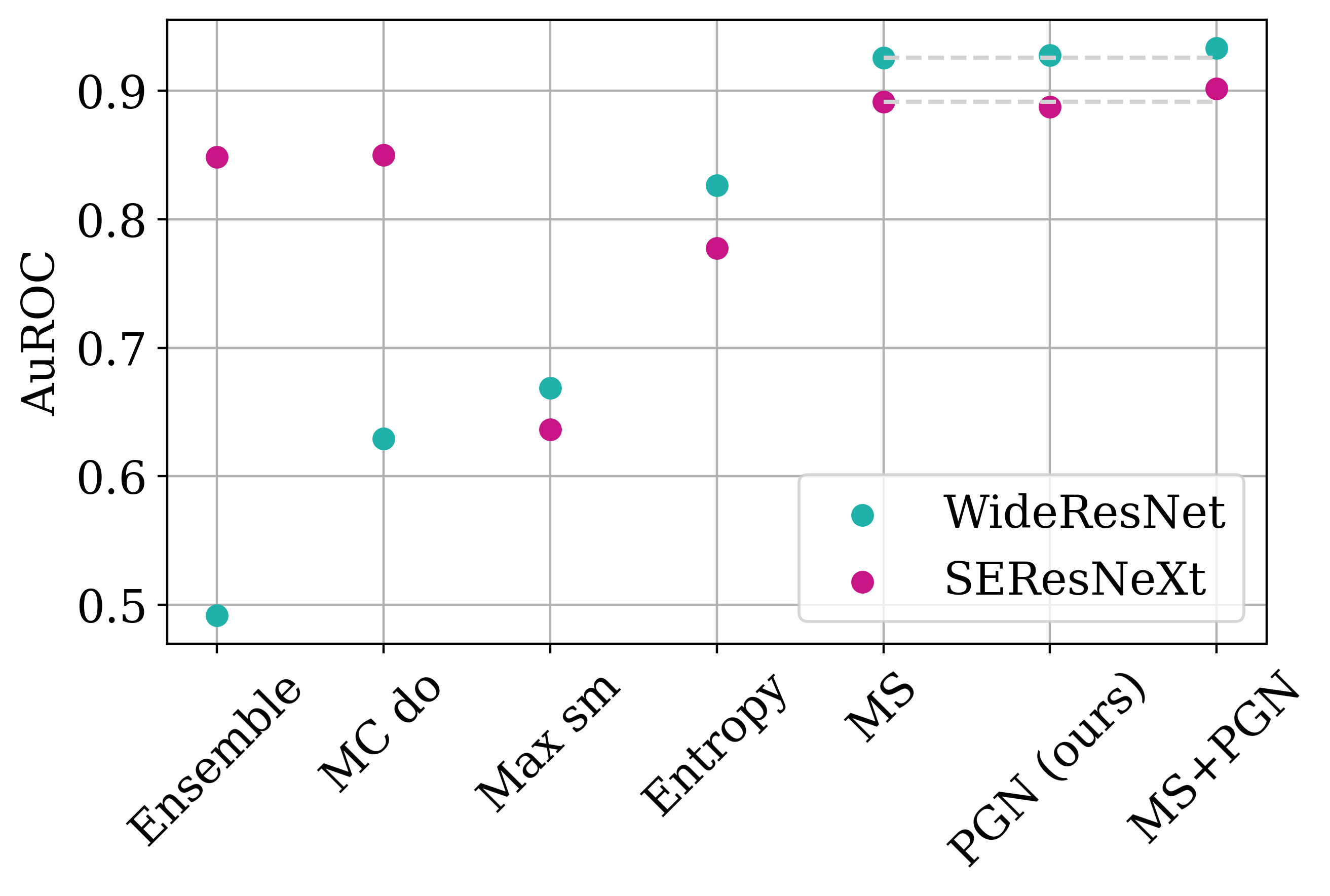
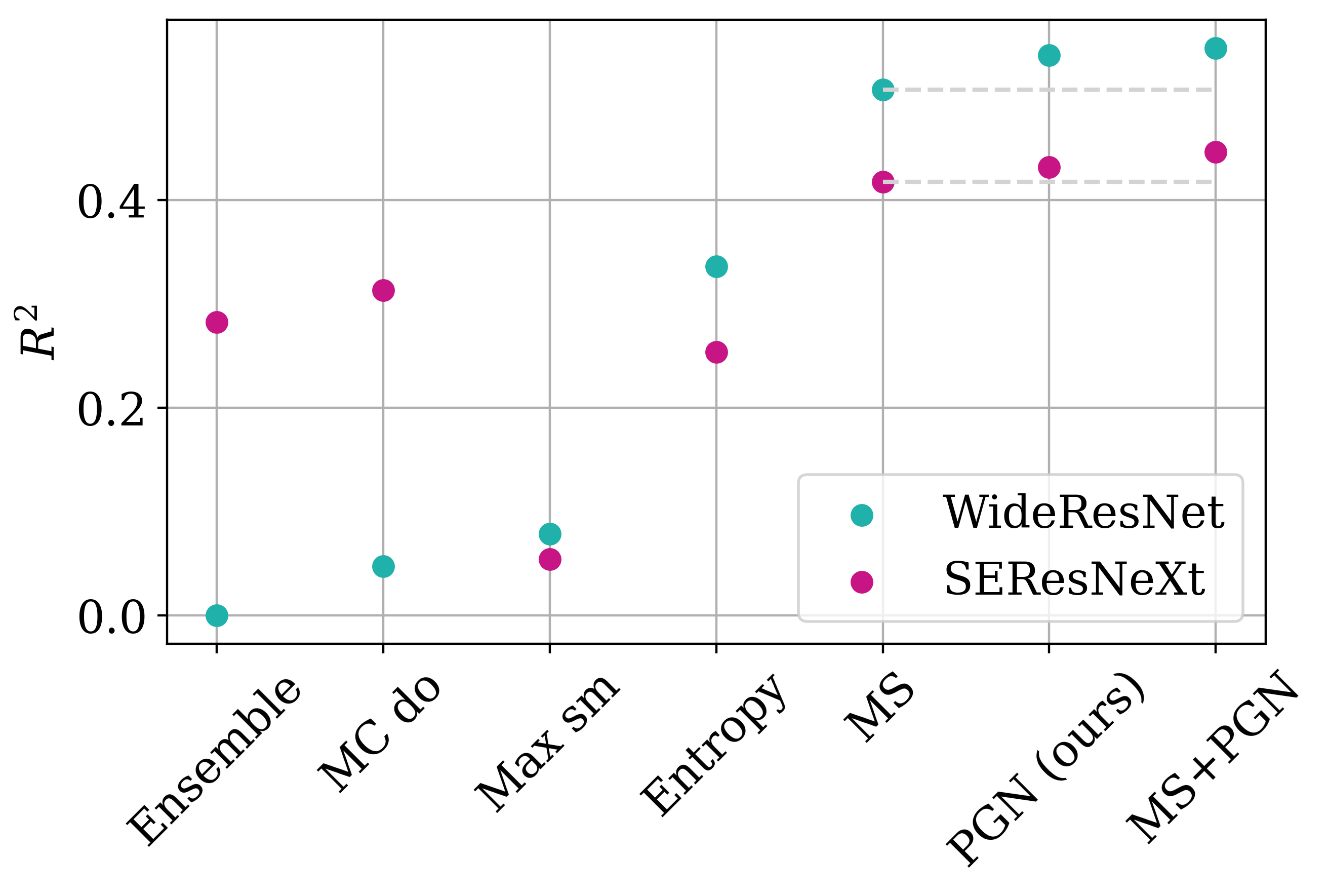
Figure 3: Segment-wise uncertainty evaluation results for both backbone architectures and the Cityscapes dataset in terms of classification AuROC and regression $R^{2}$ values. From left to right: ensemble, MC Dropout, maximum softmax, mean entropy, MetaSeg (MS) approach, gradient features obtained by predictive one-hot and uniform labels (PGN), MetaSeg in combination with PGN.

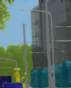
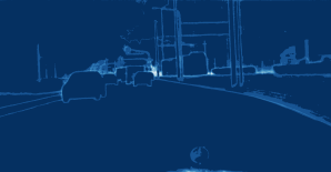
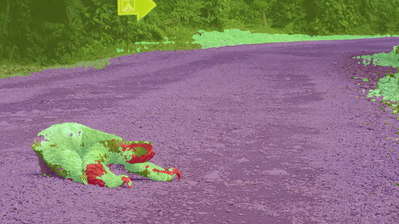
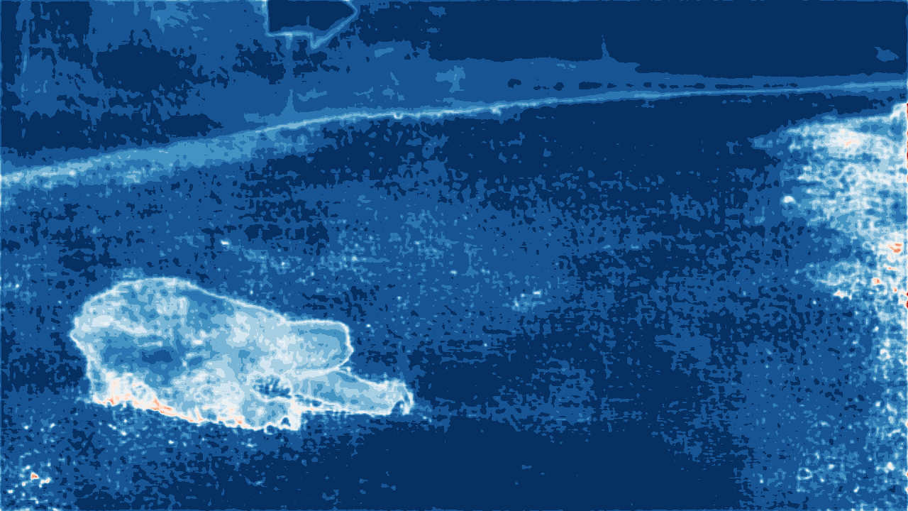
Figure 4: Semantic segmentation prediction and $\mathrm{PGN}_{\mathit{uni}}^{p=0.5}$ heatmap for the Cityscapes dataset (left) and the RoadAnomaly21 dataset (right) for the WideResNet backbone.

Table 2: OoD segmentation benchmark results for the LostAndFound and the RoadObstacle21 dataset.

	OoD data	OoD arch	adversarial	LostAndFound test-NoKnown					RoadObstacle21
				AuPRC $\uparrow$	FPR95 $\downarrow$	$\overline{\text{sIoU}}$ $\uparrow$	$\overline{\text{PPV}}$ $\uparrow$	$\overline{F_{1}}$ $\uparrow$	AuPRC $\uparrow$	FPR95 $\downarrow$	$\overline{\text{sIoU}}$ $\uparrow$	$\overline{\text{PPV}}$ $\uparrow$	$\overline{F_{1}}$ $\uparrow$
Void Classifier	$\checkmark$			$4.8$	$47.0$	$1.8$	$35.1$	$1.9$	$10.4$	$41.5$	$6.3$	$20.3$	$5.4$
Maximized Entropy	$\checkmark$	($\checkmark$)		$77.9$	$9.7$	$\mathbf{45.9}$	$63.1$	$\mathbf{49.9}$	$\mathbf{85.1}$	$\mathbf{0.8}$	$\mathbf{47.9}$	$\mathbf{62.6}$	$\mathbf{48.5}$
SynBoost	$\checkmark$	$\checkmark$		$\mathbf{81.7}$	$\mathbf{4.6}$	$36.8$	$\mathbf{72.3}$	$48.7$	$71.3$	$3.2$	$44.3$	$41.8$	$37.6$
Image Resynthesis		$\checkmark$		$57.1$	$8.8$	$27.2$	$30.7$	$19.2$	$37.7$	$4.7$	$16.6$	$20.5$	$8.4$
Embedding Density		$\checkmark$		$61.7$	$10.4$	$37.8$	$35.2$	$27.6$	$0.8$	$46.4$	$35.6$	$2.9$	$2.3$
ODIN			$\checkmark$	$52.9$	$30.0$	$39.8$	$49.3$	$34.5$	$22.1$	$15.3$	$21.6$	$18.5$	$9.4$
Mahalanobis			$\checkmark$	$55.0$	$12.9$	$33.8$	$31.7$	$22.1$	$20.9$	$13.1$	$13.5$	$21.8$	$4.7$
Ensemble		($\checkmark$)		$2.9$	$82.0$	$6.7$	$7.6$	$2.7$	$1.1$	$77.2$	$8.6$	$4.7$	$1.3$
MC Dropout		($\checkmark$)		$36.8$	$35.6$	$17.4$	$34.7$	$13.0$	$4.9$	$50.3$	$5.5$	$5.8$	$1.1$
Maximum Softmax				$30.1$	$33.2$	$14.2$	$\mathbf{62.2}$	$10.3$	$15.7$	$16.6$	$19.7$	$15.9$	$6.3$
Entropy				$52.0$	$30.0$	$40.4$	$53.8$	$42.4$	$\mathbf{20.6}$	$\mathbf{16.3}$	$\mathbf{21.4}$	$\mathbf{19.5}$	$\mathbf{10.4}$
$\mathrm{PGN}_{\mathit{uni}}^{p=0.5}$ (ours)				$\mathbf{69.3}$	$\mathbf{9.8}$	$\mathbf{50.0}$	$44.8$	$\mathbf{45.4}$	$16.5$	$19.7$	$19.5$	$14.8$	$7.4$

Table 3: OoD segmentation benchmark results for the Fishyscapes LostAndFound and the RoadAnomaly21 dataset.

	OoD data	OoD arch	adversarial	Fishyscapes LostAndFound					RoadAnomaly21
				AuPRC $\uparrow$	FPR95 $\downarrow$	$\overline{\text{sIoU}}$ $\uparrow$	$\overline{\text{PPV}}$ $\uparrow$	$\overline{F_{1}}$ $\uparrow$	AuPRC $\uparrow$	FPR95 $\downarrow$	$\overline{\text{sIoU}}$ $\uparrow$	$\overline{\text{PPV}}$ $\uparrow$	$\overline{F_{1}}$ $\uparrow$
Void Classifier	$\checkmark$			$11.7$	$15.3$	$9.2$	$39.1$	$14.9$	$36.6$	$63.5$	$21.1$	$22.1$	$6.5$
Maximized Entropy	$\checkmark$	($\checkmark$)		$44.3$	$37.7$	$21.1$	$\mathbf{48.6}$	$30.0$	$\mathbf{85.5}$	$\mathbf{15.0}$	$\mathbf{49.2}$	$\mathbf{39.5}$	$\mathbf{28.7}$
SynBoost	$\checkmark$	$\checkmark$		$\mathbf{64.9}$	$30.9$	$\mathbf{27.9}$	$\mathbf{48.6}$	$\mathbf{38.0}$	$56.4$	$61.9$	$34.7$	$17.8$	$10.0$
Image Resynthesis		$\checkmark$		$5.1$	$29.8$	$5.1$	$12.6$	$4.1$	$52.3$	$25.9$	$39.7$	$11.0$	$12.5$
Embedding Density		$\checkmark$		$8.9$	$42.2$	$5.9$	$10.8$	$4.9$	$37.5$	$70.8$	$33.9$	$20.5$	$7.9$
ODIN			$\checkmark$	$15.5$	$38.4$	$9.9$	$21.9$	$9.7$	$33.1$	$71.7$	$19.5$	$17.9$	$5.2$
Mahalanobis			$\checkmark$	$32.9$	$\mathbf{8.7}$	$19.6$	$29.4$	$19.2$	$20.0$	$87.0$	$14.8$	$10.2$	$2.7$
Ensemble		($\checkmark$)		$0.3$	$90.4$	$3.1$	$1.1$	$0.4$	$17.7$	$91.1$	$16.4$	$20.8$	$3.4$
MC Dropout		($\checkmark$)		$14.4$	$47.8$	$4.8$	$18.1$	$4.3$	$28.9$	$69.5$	$20.5$	$17.3$	$4.3$
Maximum Softmax				$5.6$	$40.5$	$3.5$	$9.5$	$1.8$	$28.0$	$72.1$	$15.5$	$15.3$	$5.4$
Entropy				$14.0$	$39.3$	$8.0$	$17.5$	$7.7$	$31.6$	$71.9$	$15.7$	$18.4$	$4.2$
$\mathrm{PGN}_{\mathit{uni}}^{p=0.5}$ (ours)				$\mathbf{26.9}$	$\mathbf{36.6}$	$\mathbf{14.8}$	$\mathbf{29.6}$	$\mathbf{16.5}$	$\mathbf{42.8}$	$\mathbf{56.4}$	$\mathbf{25.8}$	$\mathbf{21.8}$	$\mathbf{9.7}$

Table 4: Runtime measurements in seconds per frame for each method; standard deviations taken over samples in the Cityscapes validation dataset.

sec. per frame $\downarrow$	WideResNet	SEResNeXt
Softmax	$3.02\pm 0.18$	$1.08\pm 0.04$
MC Dropout	$7.52\pm 0.35$	$2.31\pm 0.10$
$\text{PGN}_{\mathit{oh}}+\text{PGN}_{\mathit{uni}}$ (ours)	$3.05\pm 0.16$	$1.09\pm 0.05$

To reduce the number of FP predictions and to estimate the prediction quality, we use meta classification and meta regression introduced by [Rottmann et al., 2020]. As input for the post-processing models, the authors use information from the network’s softmax output which characterize uncertainty and geometry of a given segment like the segment size. The degree of randomness in semantic segmentation prediction is quantified by pixel-wise quantities, like entropy and probability margin. Segment-wise features are generated from these quantities via average pooling. These MetaSeg features used in [Rottmann et al., 2020] serve as a baseline in our tests.

Similarly, we construct segment-wise features from our pixel-wise gradient $p$-norms for $p\in\{0.1,0.3,0.5,1,2\}$. We compute the mean and the variance of these pixel-wise values over a given segment. These features per segment are considered also for the inner and the boundary since the gradient scores may be higher on the boundary of a segment, see Figure 1 (bottom). The inner of the segment consists of all pixels whose eight neighboring pixels are also elements of the same segment. Furthermore, we define some relative mean and variance features over the inner and boundary which characterizes the degree of fractality. These hand-crafted quantities form a structured dataset where the columns correspond to features and the rows to predicted segments which serve as input to the post-processing models. Details on the construction of these features can be found in Appendix B.

We determine the prediction accuracy of semantic segmentation networks with respect to the ground truth via the segment-wise intersection over union (IoU, [Jaccard, 1912]). On the one hand, we perform the direct prediction of the IoU (meta regression) which serves as prediction quality estimate. On the other hand, we discriminate between $\text{IoU}=0$ (FP) and $\text{IoU}>0$ (true positive) (meta classification). We use linear classification and regression models.

For the evaluation, we use AuROC (area under the receiver operating characteristic) for meta classification and determination coefficient $R^{2}$ for meta regression. As baselines, we employ an ensemble, MC Dropout, maximum softmax probability, entropy and the MetaSeg framework. A comparison of these methods and our approach for the Cityscapes dataset is given in Figure 3. We outperform all baselines with the only exception of meta classification for the SEResNeXt backbone where MetaSeg achieves a marginal $0.41$ pp higher AuROC value than ours. Such a post-processing model captures all the information which is contained in the network’s output. Therefore, matching the MetaSeg performance by a gradient heatmap is a substantial achievement for a predictive uncertainty method. Moreover, we enhance the MetaSeg performance for both networks and both tasks combining the MetaSeg features with PGN by up to $1.02$ pp for meta classification and up to $3.98$ pp for meta regression. This indicates that gradient features contain information which is partially orthogonal to the information contained in the softmax output. Especially, the highest AuROC value of $93.31\%$ achieved for the WideResNet backbone, shows the capability of our approach to estimate the prediction quality and filter out FP predictions on the segment-level for in-distribution data.

OoD Segmentation.

Figure 4 shows segmentation predictions of the pre-trained DeepLabv3+ network with the WideResNet38 backbone together with its corresponding $\text{PGN}_{\mathit{uni}}^{p=0.5}$-heatmap. The two panels on the left show an in-distribution prediction on Cityscapes where uncertainty is mainly concentrated around segmentation boundaries which are always subject to high prediction uncertainty. Moreover, we see some false predictions in the far distance around the street crossing which can be found as a region of high gradient norm in the heatmap. In the two panels to the right, we see an OoD prediction from the RoadAnomaly21 dataset of a sloth crossing the street which is classified as part vegetation, terrain and person. The outline of the segmented sloth can be seen brightly in the gradient norm heatmap to the right indicating clear separation.

Our results in OoD segmentation are based on the evaluation protocol of the official SegmentMeIfYouCan benchmark [Chan et al., 2021a]. Evaluation on the pixel-level involves the threshold-independent area under precision-recall curve (AuPRC) and the false positive rate at the point of $0.95$ true positive rate ($\text{FPR}_{95}$). The latter constitutes an interpretable choice of operating point for each method where a minimum true positive fraction is dictated. On segment-level, an adjusted version of the mean intersection over union (sIoU) representing the accuracy of the segmentation obtained by thresholding at a particular point, positive predictive value (PPV or precision) playing the role of binary instance-wise accuracy and the $F_{1}$-score. The latter segment-wise metrics are averaged over thresholds between $0.25$ and $0.75$ with a step size of $0.05$ leading to the quantities $\overline{\text{sIoU}}$, $\overline{\text{PPV}}$ and $\overline{F_{1}}$.

Here, we compare the gradient scores of $\text{PGN}_{\mathit{uni}}$ as an OoD score against all other methods from the benchmark which provide evaluation results on all given datasets. Note, we include a table of methods with incomplete results in Appendix C. We restrict ourselves to $\text{PGN}_{\mathit{uni}}$ since we suspect it performs especially well in OoD segmentation as explained in Section 3. The results are based on evaluation files submitted to the public benchmark and are, therefore, deterministic. As baselines, we also include the same methods as for error detection before since these constitute a fitting comparison. Note, that the standard entropy baseline is not featured in the official leaderboard, so we report our own results obtained by the softmax entropy with the WideResNet backbone which performed better.

The results verified by the official benchmark are compiled in Table 2 and Table 3. We separate both tables into two halves. The bottom half contains methods with similar requirements as our method while the top half contains the stronger OoD segmentation methods which may have heavy additional requirements such as auxiliary data, architectural changes, retraining or the computation of adversarial examples. Note, the best performance value of both halves of the table is marked. In the lower part, a comparison with methods which have similarly low additional requirements is shown. We mark deep ensembles and MC dropout as requiring architectural changes since they technically require re-training in order to serve as numerical approximations of a Bayesian neural network. PGN performs among the strongest methods, showing superior performance on LostAndFound test-NoKnown, Fishyscapes and the RoadAnomaly dataset. While not clearly superior to the Entropy baseline on RoadObstacles, PGN still yields stronger performance than the deep ensemble and MC dropout baselines. Especially in Table 3, the methods in the lower part are significantly weaker w.r.t. most of the computed metrics.

The upper part of the table provides results for other OoD segmentation methods utilizing adversarial samples (ODIN [Liang et al., 2018] and Mahalanobis [Lee et al., 2018]), OoD data (Void Classifier [Blum et al., 2019b], Maximized Entropy [Chan et al., 2021b] and SynBoost [Biase et al., 2021]) or auxiliary models (SynBoost, Image Resynthesis [Lis et al., 2019] and Embedding Density [Blum et al., 2019b]). Note, that the Maximized Entropy method does not modify the network architecture, but uses another loss function requiring retraining. In several cases, we find that our method is competitive with some of the stronger methods. We outperform the two adversarial-based methods for the LostAndFound as well as the RoadAnomaly21 dataset. In detail, we obtain AuPRC values up to $22.8$ pp higher on segment-level and $\overline{F_{1}}$ values values up to $24.8$ pp higher on pixel-level. For the other two datasets we achieve similar results. Furthermore, we beat the Void Classifier method, that uses OoD data during training, in most cases. We improve the AuPRC metric by up to $64.5$ pp and the $\overline{\text{sIoU}}$ metric by up to $48.2$ pp, both for the LostAndFound dataset. In addition, our gradient norm outperforms in many cases the Image Resynthesis as well as the Embedding Density approach which are based on an external reconstruction model followed by a discrepancy network and normalizing flows, respectively. Summing up, we have shown superior OoD segmentation performance in comparison to the other uncertainty based methods and outperform some of the more complex approaches (using OoD data, adversarial samples or generative models).

Computational Runtime.

Lastly, we demonstrate the computational efficiency of our method and show runtime measurements for the network forward pass (“Softmax”), MC dropout ($25$ samples) and computing both, $\text{PGN}_{\mathit{oh}}$ and $\text{PGN}_{\mathit{uni}}$, in Table 4. While sampling MC dropout requires over twice the time per frame for both backbone networks, the computation of $\text{PGN}_{\mathit{oh}}+\text{PGN}_{\mathit{uni}}$ only leads to a marginal computational overhead of around $1\%$ due to consisting only of tensor multiplications. Note, that the entropy baseline requires roughly the same compute as Softmax and deep ensembles tend to be slower than MC dropout due to partial parallel computation. The measurements were each made on a single Nvidia Quadro P6000 GPU.

Limitations.

We declare that our method is merely on-par with other uncertainty quantification methods for pixel-level considerations but outperforming well-known methods such as MC Dropout. For segment-wise error detection, our approach showed improved results. Moreover, there have been some submissions to the SegmentMeIfYouCan benchmark (requiring OoD data, re-training or complex auxiliary models) which outperform our method. However, a direct application of the methods is barely possible if suitable OoD data have to pass into the training or auxiliary models are used in combination with the segmentation network, which also increases the runtime during application, in comparison to our simple and flexible method. Note, our approach has one light architectural restrictions, i.e., the final layer has to be a convolution, but this is in general common for segmentation models.

5 CONCLUSION

In this work, we presented an efficient method of computing gradient uncertainty scores for a wide class of deep semantic segmentation models. Moreover, we appreciate a low computational cost associated with them. Our experiments show that large gradient norms obtained by our method statistically correspond to erroneous predictions already on the pixel-level and can be normalized such that they yield similarly calibrated confidence measures as the maximum softmax score of the model. On a segment-level our method shows considerable improvement in terms of error detection. Gradient scores can be utilized to segment out-of-distribution objects significantly better than sampling- or any other output-based method on the SegmentMeIfYouCan benchmark and has competitive results with a variety of methods, in several cases clearly outperforming all of them while coming at negligible computational overhead. We hope that our contributions in this work and the insights into the computation of pixel-wise gradient feedback for segmentation models will inspire future work in uncertainty quantification and pixel-wise loss analysis.

APPENDIX

Appendix A Computational Derivations and Implementation Details

A.1 Computations

In this work we assume that the final activation in the segmentation network is given by a softmax activation of categorical features $\phi$ in the last layer

$$\varSigma^{j}(\phi)=\frac{\mathrm{e}^{\phi^{j}}}{\sum_{i=1}^{C}\mathrm{e}^{\phi^{i}}}$$ (7)

where $C$ is the number of classes and $\phi=\phi(\theta)$ is now dependent on a set of parameters $\theta$. In order to compute the gradients of the categorical cross entropy at pixel $(a,b)$ given any auxiliary label $y$

$$\mathcal{L}_{ab}(\phi(\theta)\|y)=-\sum_{j=1}^{C}y_{ab,j}\log(\varSigma^{j}(\phi_{ab}(\theta))),$$ (8)

we require the derivative of the softmax function

$$\begin{split}\nabla_{\!\theta}\varSigma^{j}(\phi(\theta))=&\frac{\mathrm{e}^{\phi^{j}}\nabla_{\!\theta}\phi^{j}}{\sum_{i=1}^{C}\mathrm{e}^{\phi^{i}}}-\frac{\mathrm{e}^{\phi^{j}}\sum_{k=1}^{C}\mathrm{e}^{\phi^{k}}\nabla_{\!\theta}\phi^{k}}{\left(\sum_{i=1}^{C}\mathrm{e}^{\phi^{i}}\right)^{2}}\\ =&\varSigma^{j}(\phi)\cdot\nabla_{\!\theta}\phi^{j}\sum_{k=1}^{C}\varSigma^{k}(\phi)\\ &-\varSigma^{j}(\phi)\sum_{k=1}^{C}\varSigma^{k}(\phi)\cdot\nabla_{\!\theta}\phi^{k}\\ =&\varSigma^{j}(\phi)\left(\sum_{k=1}^{C}\varSigma^{k}(\phi)\cdot\nabla_{\!\theta}\phi^{j}-\varSigma^{k}\nabla_{\!\theta}\phi^{k}\right)\\ =&\varSigma^{j}(\phi)\sum_{k=1}^{C}\varSigma^{k}(\phi)(\delta_{kj}-1)\nabla_{\!\theta}\phi^{k}.\end{split}$$ (9)

Note, that the auxiliary label $y\in[0,1]^{C}$ may be anything, e.g., actual ground truth information about pixel $(a,b)$, the predicted probability distribution at that location, the one-hot encoded prediction or a uniform class distribution. In the following, we regard $y$ to be independent of $\phi$. The gradient of the cross entropy loss is

$$\begin{split}\nabla_{\!\theta}\mathcal{L}_{ab}(\phi(\theta)\|y)=&-\sum_{j=1}^{C}y_{ab,j}\frac{1}{\varSigma^{j}(\phi_{ab})}\nabla_{\!\theta}\varSigma^{j}(\phi_{ab})\\ =&\sum_{j=1}^{C}\sum_{k=1}^{C}(y_{ab,j}\varSigma^{k}(\phi_{ab})\\ &-y_{j}\varSigma^{k}(\phi_{ab})\delta_{kj})\cdot\nabla_{\!\theta}\phi^{k}_{ab}(\theta)\\ =&\sum_{k=1}^{C}\varSigma^{k}(\phi_{ab})(1-y_{k})\cdot\nabla_{\!\theta}\phi^{k}_{ab}(\theta).\end{split}$$ (10)

The feature maps are the result of convolution $\mathcal{C}_{K,\beta}$ against a filter bank $K\in\mathcal{R}^{\kappa_{\mathrm{in}}\times\kappa_{\mathrm{out}}\times(2s+1)\times(2s+1)}$ and addition of a bias vector $\beta\in\mathcal{R}^{\kappa_{\mathrm{out}}}$. Here, $\kappa_{\mathrm{in}}$ and $\kappa_{\mathrm{out}}$ denote the number of in- and out-going channels, respectively. $K$ has parameters $(K_{e}^{h})_{fg}$ where $e$ and $h$ indicate in- and out-going channels respectively and $f$ and $g$ index the spatial filter position. In particular, we obtain the value $\phi_{ab}^{d}$ at pixel location $(a,b)$ in channel $d$ by

$$\begin{split}\phi_{ab}^{d}(K,\beta,\psi)=&[\mathcal{C}_{K,\beta}(\psi)]_{ab}^{d}=(K\ast\psi)_{ab}^{d}+\beta^{d}\\ =&\sum_{c=1}^{\kappa_{\mathrm{in}}}\sum_{q=-s}^{s}\sum_{r=-s}^{s}(K_{c}^{d})_{qr}\psi^{c}_{a+q,b+r}+\beta^{d}.\end{split}$$ (11)

Here, we assume the filters of size $(2s+1)\times(2s+1)$ indexed symmetrically around their center and $\psi$ is the feature map pre-convolution. Note, also that the bias is constant across the indices $a$ and $b$. Taking explicit derivatives of this expression with respect to one of the parameters in $K$ yields

$$\begin{split}\frac{\partial(K\ast\phi)_{ab}^{d}}{\partial(K_{e}^{h})_{fg}}=&\sum_{c=1}^{\kappa_{\mathrm{in}}}\sum_{q,r=-s}^{s}\frac{\partial(K_{c}^{d})_{qr}}{\partial(K_{e}^{h})_{fg}}\,\psi_{a+q,b+r}^{c}\\ =&\sum_{c=1}^{\kappa_{\mathrm{in}}}\sum_{q,r=-s}^{s}\delta^{dh}\delta_{ce}\delta_{pf}\delta_{qg}\psi_{a+q,b+r}^{c}\\ =&\delta^{dh}\psi_{a+f,b+g}^{e}.\end{split}$$ (12)

When utilizing the predicted one-hot vector (self-learning gradient), i.e., $y^{\mathit{oh}}_{k}=\delta_{k\hat{c}}$ and using the fact that the last-layer convolution is $(1\times 1)$, we obtain

$$\begin{split}\frac{\partial}{\partial K_{e}^{f}}\mathcal{L}_{ab}=&\sum_{k=1}^{C}\varSigma^{k}(\phi_{ab})(1-\delta_{k\hat{c}})\frac{\partial\phi_{ab}^{k}}{\partial K_{e}^{f}}\\ =&\varSigma^{f}(\phi_{ab})(1-\delta_{f\hat{c}})\psi_{ab}^{e}\end{split}$$ (13)

while the uniform categorical label $y_{k}=\tfrac{1}{C}$ yields

$$\begin{split}\frac{\partial}{\partial K_{e}^{f}}\mathcal{L}_{ab}=&\sum_{k=1}^{C}\varSigma^{k}(\phi_{ab})\left(1-\frac{1}{C}\right)\cdot\nabla_{\!\theta}\phi^{k}_{ab}(\theta)\\ =&\frac{C-1}{C}\varSigma^{f}(\phi_{ab})\psi_{ab}^{e}.\end{split}$$ (14)

A.2 Computing Deeper Gradients via Explicit Backpropagation

While for the last-layer gradients the computation from above simplifies significantly due to the fact that pixel-wise gradients only depend on the feature map values at the same pixel-location. Deeper layers are usually not $(1\times 1)$, so the forward pass couples feature map values over a larger receptive field, e.g., $(3\times 3)$. However, gradients for the second-to-last layer can still be computed with comparably small effort by extracting feature map patches via the unfold function. Here, we consider a DeepLabv3+ implementation¹ [Zhu et al., 2019] for which the feature maps depend in the following way on the weights of the second-to-last layer $T-1$ (where $T$ indicates the last layer):

$$\phi(K_{T-1})=\mathcal{C}_{K_{T},\beta_{T}}\circ\mathsf{ReLU}\circ\mathsf{BN}_{T}\circ\mathcal{C}_{K_{T-1},\beta_{T-1}}(\psi_{T-1}),$$ (15)

where $\mathsf{BN}_{T}$ is a batch normalization layer and $\psi_{T-1}$ are the features prior to the convolution $\mathcal{C}_{K_{T-1},\beta_{T-1}}$ in question. With fully expanded indices, this amounts to

$$\begin{split}\phi_{ab}^{d}=&\sum_{k_{T}}K_{k_{T}}^{d}\mathsf{ReLU}\Biggl{(}\mathsf{BN}_{T}\Biggl{[}\sum_{k_{T-1}}\sum_{q,r}\left((K_{T-1})_{k_{T-1}}^{k_{T}}\right)_{qr}\\ &(\psi_{T-1})_{a+q,b+r}^{k_{T-1}}+\beta_{T-1}^{k_{T}}\biggr{]}\Biggr{)}+\beta_{T}^{d}\end{split}$$ (16)

with $k_{T}$, $k_{T-1}$ indexing the respective amount of channels and $q,r$ indexing the filter coordinates of $K_{T-1}$. Note, that we still assume here that the last convolutional layer has spatial extent 0 into both directions, so $K_{T}\in\mathcal{R}^{\kappa_{\mathrm{in}}\times C\times 1\times 1}$. The chain rule for this forward pass is then

$$\begin{split}&\frac{\partial\phi_{ab}^{d}}{\partial((K_{T-1})_{e}^{f})_{gh}}=\sum_{k_{T}}K_{k_{T}}^{d}\mathsf{ReLU}^{\prime}(\cdot)\cdot\mathsf{BN}_{T}^{\prime}\\ &\ \ \ \ \ \ \cdot\left(\sum_{k_{T-1}}\sum_{q,r}\frac{\partial((K_{T-1})_{k_{T-1}}^{k_{T}})_{qr}}{\partial((K_{T-1})_{e}^{f})_{gh}}(\psi_{T-1})_{a+q,b+r}^{k_{T-1}}\right)\\ &\ \ \ \ =\sum_{k_{T}}K_{k_{T}}^{d}\mathsf{ReLU}^{\prime}(\cdot)\cdot\mathsf{BN}^{\prime}_{T}\\ &\ \ \ \ \ \ \cdot\sum_{k_{T-1}}\sum_{q,r}\delta^{k_{T}f}\delta_{k_{T-1}e}\delta_{gp}\delta_{hq}(\psi_{T-1})_{a+q,b+r}^{k_{T-1}}\\ &\ \ \ \ =K_{f}^{d}(\mathsf{ReLU}^{\prime})_{ab}^{f}\cdot(\mathsf{BN}^{\prime}_{T})_{ab}^{f}\cdot(\psi_{T-1})_{a+g,b+h}^{e}.\end{split}$$ (17)

The term with the derivative of the $\mathsf{ReLU}$ activation is simply the Heaviside function evaluated at the features pre-activation which have been computed in the forward pass anyway (the discontinuity at zero has vanishing probability of an evaluation). The derivative of the batch normalization layer is multiplication by the linear batch norm parameter which is applied channel-wise. The running indices $g$ and $h$ only apply to the last factor which can be computationally treated by extracting $(3\times 3)$-patches from $\psi_{T-1}$ using the unfold operation. In computing the norm of $\nabla_{K_{T-1}}\phi_{ab}^{d}$ with respect to the indices $e$, $f$, $g$ and $h$, we note that the expression in eq. (17) is a product of two tensors $S_{f}\cdot\Psi_{gh}^{e}$ for each pixel $(a,b)$. $L^{p}$-norms of such tensors $T_{ij}=S_{i}\Psi_{j}$ factorize which makes their computation feasible:

$$\begin{split}\|T\|_{p}=&\left(\sum_{i,j}|T_{ij}|^{p}\right)^{\frac{1}{p}}=\left(\sum_{i,j}|S_{i}|^{p}|\Psi_{j}|^{p}\right)^{\frac{1}{p}}\\ =&\left(\sum_{i}\left[|S_{i}|^{p}\sum_{j}|\Psi_{j}|^{p}\right]\right)^{\frac{1}{p}}=\|S\|_{p}\|\Psi\|_{p}.\end{split}$$ (18)

Appendix B Details on the Feature Construction for Segment-wise Prediction Quality Estimation

The tasks of meta classification (false positive detection) and meta regression (prediction quality estimation) based on uncertainty measures extracted from the network’s softmax output were introduced in [Rottmann et al., 2020]. The neural network provides for each pixel $z$ given an input image $x$ a probability distribution $f_{z}(y|x)$ over a label space $C=\{y_{1},\ldots,y_{c}\}$, with $y\in C$. The degree of randomness in the semantic segmentation prediction $f_{z}(y|x)$ is quantified by pixel-wise dispersion measures, like entropy

$$E_{z}(x)=-\frac{1}{\log(c)}\sum_{y\in\mathcal{C}}f_{z}(y|x)\log f_{z}(y|x)$$ (19)

and probability margin

$$M_{z}(x)=1-f_{z}(\hat{y}_{z}(x)|x)+\max_{y\in\mathcal{C}\setminus\{\hat{y}_{z}(x)\}}f_{z}(y|x)$$ (20)

where

$$\hat{y}_{z}(x)=\operatorname*{arg\,max}_{y\in\mathcal{C}}f_{z}(y|x)$$ (21)

is the predicted class for each pixel $z$. To obtain segment-wise features from these dispersion measures which characterize uncertainty, they are aggregated over segments via average pooling obtaining mean dispersions $\mu E$ and $\mu M$. As erroneous or poor predictions oftentimes have fractal segment shapes, it is distinguished between the inner of the segment (consisting of all pixels whose eight neighboring pixels are also elements of this segment) and the boundary. This results in segment size $S$ and mean dispersion features per segment also for the inner (in) and the boundary (bd). Furthermore, relative segment sizes $\tilde{S}=S/S_{bd}$ and $\tilde{S}_{in}=S_{in}/S_{bd}$ as well as relative mean dispersions $\mu\tilde{D}=\mu D\tilde{S}$ and $\mu\tilde{D}_{in}=\mu D_{in}\tilde{S}_{in}$ where $D\in\{E,M\}$ are defined. Moreover, the mean class probabilities $P(y)$ for each class $y\in C$ are added resulting in the set of hand-crafted features

$$\begin{split}&\{S,S_{in},S_{bd},\tilde{S},\tilde{S}_{in}\}\cup\{P(y)\,:\,y=1,\ldots,c\}\\ &\cup\{\mu D,\mu D_{in},\mu D_{bd},\mu\tilde{D},\mu\tilde{D}_{in}\,:\,D\in\{E,M\}\}\,.\end{split}$$ (22)

These features serve as a baseline in our tests.

The computed gradients in Section 3 with applied $p$-norm, $p\in\{0.1,0.3,0.5,1,2\}$, are denoted by $G_{z}^{p=\#}(x)$, $\#\in\{0.1,0.3,0.5,1,2\}$, for image $x$. Similar to the dispersion measures, we compute the mean and additionally the variance of these pixel-wise values of a given segment to obtain $\mu G^{p=\#}$ and $vG^{p=\#}$, respectively. Since the gradient uncertainties may be higher on the boundary of a segment, the mean and variance features per segment are considered also for the inner and the boundary. Furthermore, we define relative mean and variance features to quantify the degree of fractality. This results in the following gradient features

$$\begin{split}&\{\mu G^{p=\#},\mu G_{in}^{p=\#},\mu G_{bd}^{p=\#},\mu\tilde{G}^{p=\#},\mu\tilde{G}_{in}^{p=\#},\\ &vG^{p=\#},vG_{in}^{p=\#},vG_{bd}^{p=\#},v\tilde{G}^{p=\#},v\tilde{G}_{in}^{p=\#}:\\ &\#\in\{0.1,0.3,0.5,1,2\}\}\,.\end{split}$$ (23)

Note, these features can be computed for the gradient scores obtained from the predictive one-hot ($\text{PGN}_{\mathit{oh}}$) and the uniform label ($\text{PGN}_{\mathit{uni}}$) as well as for gradients of deeper layers (see Section A.2).

Appendix C Extended OoD Segmentation Results

In Section 4.2, we have compared our approach with different OoD segmentation methods that provide a complete evaluation on the four different benchmark datasets. In Table 5 and Table 6, we provide the comparison of our method with the other approaches part of the benchmark. The incomplete results render the comparison less fair.

	LostAndFound test-NoKnown					RoadObstacle21
	AuPRC $\uparrow$	FPR95 $\downarrow$	$\overline{\text{sIoU}}$ $\uparrow$	$\overline{\text{PPV}}$ $\uparrow$	$\overline{F_{1}}$ $\uparrow$	AuPRC $\uparrow$	FPR95 $\downarrow$	$\overline{\text{sIoU}}$ $\uparrow$	$\overline{\text{PPV}}$ $\uparrow$	$\overline{F_{1}}$ $\uparrow$
PEBAL	$-$	$-$	$-$	$-$	$-$	$5.0$	$12.7$	$29.9$	$7.6$	$5.5$
DenseHybrid	$78.7$	$2.1$	$46.9$	$52.1$	$52.3$	$87.1$	$0.2$	$45.7$	$50.1$	$50.7$
RPL+CoroCL	$-$	$-$	$-$	$-$	$-$	$85.9$	$0.6$	$52.6$	$56.7$	$56.7$
EAM	$-$	$-$	$-$	$-$	$-$	$92.9$	$0.5$	$65.9$	$76.5$	$75.6$
RbA	$-$	$-$	$-$	$-$	$-$	$95.1$	$0.1$	$54.3$	$59.1$	$57.4$
Mask2Anomaly	$-$	$-$	$-$	$-$	$-$	$93.2$	$0.2$	$55.7$	$75.4$	$68.2$
Road Inpainting	$82.9$	$35.8$	$49.2$	$60.7$	$52.3$	$54.1$	$47.1$	$57.6$	$39.5$	$36.0$
NFlowJS	$89.3$	$0.7$	$54.6$	$59.7$	$61.8$	$85.6$	$0.4$	$45.5$	$49.5$	$50.4$
JSRNet	$74.2$	$6.6$	$34.3$	$45.9$	$36.0$	$28.1$	$28.9$	$18.6$	$24.5$	$11.0$
FlowEneDet	$79.8$	$2.9$	$43.8$	$52.8$	$48.1$	$73.7$	$1.0$	$42.6$	$42.3$	$40.0$
DaCUP	$81.4$	$7.4$	$38.3$	$67.3$	$51.1$	$81.5$	$1.1$	$37.7$	$60.1$	$46.0$
$\mathrm{PGN}_{\mathit{oh}}^{p=0.5}$	$64.9$	$18.4$	$48.3$	$50.0$	$46.9$	$18.8$	$14.8$	$22.1$	$16.5$	$9.2$
$\mathrm{PGN}_{\mathit{uni}}^{p=0.5}$	$69.3$	$9.8$	$50.0$	$44.8$	$45.4$	$16.5$	$19.7$	$19.5$	$14.8$	$7.4$

Table 5: OoD segmentation results for the LostAndFound and the RoadObstacle21 dataset.

	Fishyscapes LostAndFound					RoadAnomaly21
	AuPRC $\uparrow$	FPR95 $\downarrow$	$\overline{\text{sIoU}}$ $\uparrow$	$\overline{\text{PPV}}$ $\uparrow$	$\overline{F_{1}}$ $\uparrow$	AuPRC $\uparrow$	FPR95 $\downarrow$	$\overline{\text{sIoU}}$ $\uparrow$	$\overline{\text{PPV}}$ $\uparrow$	$\overline{F_{1}}$ $\uparrow$
PEBAL	$-$	$-$	$-$	$-$	$-$	$49.1$	$40.8$	$38.9$	$27.2$	$14.5$
DenseHybrid	$-$	$-$	$-$	$-$	$-$	$78.0$	$9.8$	$54.2$	$24.1$	$31.1$
RPL+CoroCL	$-$	$-$	$-$	$-$	$-$	$83.5$	$11.7$	$49.8$	$30.0$	$30.2$
EAM	$81.5$	$-$	$-$	$-$	$-$	$93.8$	$4.1$	$67.1$	$53.8$	$60.9$
RbA	$-$	$-$	$-$	$-$	$-$	$94.5$	$4.6$	$64.9$	$47.5$	$51.9$
Mask2Anomaly	$46.0$	$4.4$	$-$	$-$	$-$	$88.7$	$14.6$	$55.3$	$51.7$	$47.2$
NFlowJS	$-$	$-$	$-$	$-$	$-$	$56.9$	$34.7$	$36.9$	$18.0$	$14.9$
JSRNet	$-$	$-$	$-$	$-$	$-$	$33.6$	$43.9$	$20.2$	$29.3$	$13.7$
ObsNet	$-$	$-$	$-$	$-$	$-$	$75.4$	$26.7$	$44.2$	$52.6$	$45.1$
FlowEneDet	$-$	$-$	$-$	$-$	$-$	$36.7$	$77.8$	$15.5$	$16.8$	$3.4$
$\mathrm{PGN}_{\mathit{oh}}^{p=0.5}$	$22.8$	$35.5$	$12.1$	$27.3$	$14.1$	$39.3$	$66.5$	$23.1$	$21.5$	$7.8$
$\mathrm{PGN}_{\mathit{uni}}^{p=0.5}$	$26.9$	$36.6$	$14.8$	$29.6$	$16.5$	$42.8$	$56.4$	$25.8$	$21.8$	$9.7$

Table 6: OoD segmentation results for the Fishyscapes LostAndFound and the RoadAnomaly21 dataset.

In detail, the first block consists of approaches using OoD data, i.e., PEBAL [Tian et al., 2022], DenseHybrid [Grcic et al., 2022], RPL+CoroCL [Liu et al., 2023], EAM [Grcic et al., 2023], RbA [Nayal et al., 2023] and Mask2Anomaly [Rai et al., 2023]. The latter three methods are based on the strong vision transformer models resulting in comparatively high OoD segmentation performance. The methods of the second block use complex auxiliary/generative models, namely Road Inpainting [Lis et al., 2020], NFlowJS [Grcic et al., 2021], JSRNet [Vojir et al., 2021], ObsNet [Besnier et al., 2021], FlowEneDet [Gudovskiy et al., 2023] and DaCUP [Vojíř and Matas, 2023]. Our method shows performance values in the mid-range among the different methods for some metrics. However, these approaches require OoD data for retraining or are based on auxiliary or generative models, while our PGN module can be easily integrated into various semantic segmentation models during inference with minimal computation overhead.

Gradient scores perform perhaps the least convincingly on the RoadObstacle21 benchmark. We find a slight trend of $\text{PGN}_{\mathit{oh}}$ performing better in the Obstacle track which can be seen to be closer to in-distribution data in semantic segmentation for autonomous driving. This connection would be consistent with our finding in actual in-distribution errors, while $\text{PGN}_{\mathit{uni}}$ performs better on the Anomaly track which is more clearly out-of-distribution for street scene recognition.

Appendix D Ablation: Different $p$-norms

In this section, we present an ablation study for different $p$-norms, $p\in\{0.1,0.3,0.5,1,2\}$, that are applied to the calculated gradients of the last convolutional layer.

Pixel-wise Uncertainty Evaluation.

The area under the sparsification error curve (AuSE) is considered to access the correlation of uncertainty and prediction errors on pixel level and the expected calibration error (ECE) to assess the statistical reliability of the uncertainty measure. In Table 7 the results for the different $p$-norms in terms of these two metrics are given.

		last layer		second-to-last layer
	$p$	ECE $\downarrow$	AuSE $\downarrow$	ECE $\downarrow$	AuSE $\downarrow$
	$0.1$	$0.0187$	$0.0500$	$0.0186$	$\underline{0.0235}$
Wide-	$0.3$	$0.0183$	$0.0712$	$0.0125$	$0.0286$
ResNet	$0.5$	$0.0163$	$0.0508$	$0.0059$	$0.0280$
(one-hot)	$1$	$\underline{0.0025}$	$0.0307$	$\underline{0.0027}$	$0.0271$
	$2$	$\mathbf{0.0019}$	$\underline{0.0268}$	$\mathbf{0.0021}$	$0.0265$
	$0.1$	$0.0186$	$0.0784$	$0.0096$	$0.3347$
Wide-	$0.3$	$0.0163$	$0.3426$	$0.1846$	$0.6746$
ResNet	$0.5$	$0.0241$	$0.5857$	$0.3385$	$0.7520$
(uniform)	$1$	$0.3762$	$0.7424$	$0.4345$	$0.8028$
	$2$	$0.3868$	$0.8104$	$0.3989$	$0.8253$
	$0.1$	$0.0347$	$\mathbf{0.0201}$	$0.0344$	$\mathbf{0.0060}$
SERes-	$0.3$	$0.0336$	$0.0386$	$0.0290$	$0.0353$
NeXt	$0.5$	$0.0305$	$0.0399$	$0.0214$	$0.0379$
(one-hot)	$1$	$0.0078$	$0.0383$	$0.0079$	$0.0377$
	$2$	$0.0039$	$0.0365$	$0.0068$	$0.0365$
	$0.1$	$0.0346$	$0.0427$	$0.0295$	$0.1823$
SERes-	$0.3$	$0.0313$	$0.2484$	$0.1916$	$0.4878$
NeXt	$0.5$	$0.0076$	$0.5617$	$0.3000$	$0.6198$
(uniform)	$1$	$0.3744$	$0.7694$	$0.4075$	$0.7413$
	$2$	$0.4030$	$0.8187$	$0.4003$	$0.8116$

Table 7: Pixel-wise uncertainty evaluation results for both backbone architectures and the Cityscapes dataset as well as for different $p$-norms and layers in terms of ECE and AuSE.

We observe improved performance for the gradient scores obtained from the predictive one-hot label with respect to both metrics. These scores are better calibrated for greater values of $p$, whereas there is no clear trend for the AuSE metric. In contrast, for the gradient scores obtained from the uniform label the calibration ability as well as the sparsification error enhance mostly for decreasing values of $p$.

Segment-wise Prediction Quality Estimation.

For the segment-wise prediction quality estimation, we consider meta classification, i.e., classifying between $\text{IoU}=0$ (false positive) and $\text{IoU}>0$ (true positive), and meta regression, i.e., direct prediction of the IoU. The gradient features (see eq. (23)) which are computed for each value of $p$, also separated for predictive one-hot and uniform labels, serve as input for the meta models. The results are given in Table 8 and visualized in Figure 5. The WideResNet backbone outperforms the SEResNeXt for meta classification and regression. Moreover, higher AuROC and $R^{2}$ performances are achieved for greater values of $p$ independent of the architecture or the label (predictive one-hot or uniform) used for gradient scores computation.

		last layer		second-to-last layer
	$p$	AuROC $\uparrow$	$R^{2}$ $\uparrow$	AuROC $\uparrow$	$R^{2}$ $\uparrow$
	$0.1$	$87.66$	$19.40$	$88.40$	$29.45$
Wide-	$0.3$	$89.02$	$38.03$	$90.28$	$48.23$
ResNet	$0.5$	$90.06$	$46.82$	$90.52$	$49.63$
(one-hot)	$1$	$\mathbf{91.97}$	$\underline{50.82}$	$91.04$	$50.28$
	$2$	$\underline{91.90}$	$50.72$	$\mathbf{91.54}$	$\underline{50.54}$
	$0.1$	$87.97$	$22.65$	$89.67$	$27.99$
Wide-	$0.3$	$89.84$	$43.72$	$90.84$	$45.96$
ResNet	$0.5$	$90.66$	$48.71$	$91.08$	$48.66$
(uniform)	$1$	$91.18$	$50.26$	$\underline{91.36}$	$50.48$
	$2$	$91.77$	$\mathbf{51.48}$	$\mathbf{91.54}$	$\mathbf{51.37}$
	$0.1$	$81.65$	$12.81$	$81.48$	$2.29$
SERes-	$0.3$	$82.91$	$25.73$	$84.80$	$32.56$
NeXt	$0.5$	$84.24$	$33.43$	$85.28$	$36.21$
(one-hot)	$1$	$85.68$	$38.57$	$86.01$	$38.03$
	$2$	$87.70$	$39.08$	$87.82$	$39.00$
	$0.1$	$81.90$	$14.41$	$78.49$	$6.06$
SERes-	$0.3$	$83.91$	$30.44$	$85.14$	$28.28$
NeXt	$0.5$	$85.51$	$35.40$	$85.62$	$33.40$
(uniform)	$1$	$86.46$	$37.61$	$86.38$	$38.05$
	$2$	$87.30$	$40.54$	$87.31$	$40.38$

Table 8: Segment-wise uncertainty evaluation results for both backbone architectures and the Cityscapes dataset as well as for the different $p$-norms and layers in terms of classification AuROC and regression $R^{2}$.

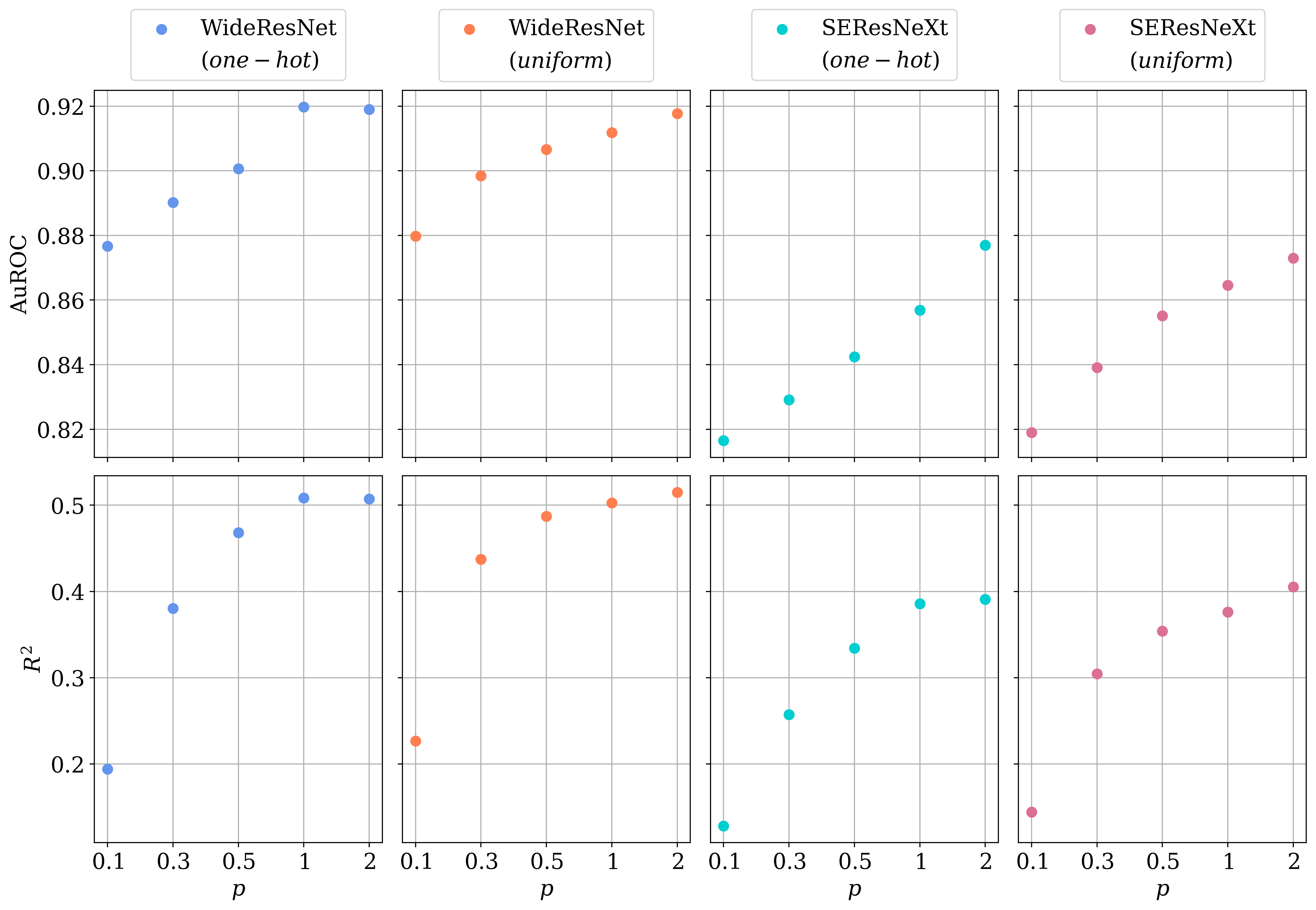
Figure 5: AuROC and $R^{2}$ values for both backbone architectures applied to the Cityscapes dataset and the different $p$-norms.

OoD Segmentation.

Our approach provides pixel-wise uncertainty scores obtained by computing the partial norm. In Figure 6 the pixel-wise heatmaps for both backbones, different $p$-norms and the predictive one-hot as well as the uniform label are shown.

Figure 6: Ground truth (labeled OoD object), semantic segmentation prediction and PGN heatmaps for different $p$-norms as well as for the predictive one-hot and the uniform label, respectively.

We observe that for higher $p$ values the number of uncertain pixels increases, the gradients are more sensitive to unconfident predictions. For a $p$ value of $0.1$ only a few pixels of OoD object have high uncertainty while the background is completely certain. For values of $p=1$ and $p=2$, in particular using the uniform label, the gradient scores show higher uncertainties in more sectors. To identify out-of-distribution regions, we threshold per pixel on our gradient scores, i.e., high uncertainty corresponds to out-of-distribution. Here, the OoD objects are mostly covered (and not so many background pixels) for $p$ values of $0.3$ and $0.5$. These observations are reflected in the OoD segmentation results, given in Table 9 and Table 10.

		LostAndFound					RoadObstacle21
	$p$	AuPRC $\uparrow$	FPR95 $\downarrow$	$\overline{\text{sIoU}}$ $\uparrow$	$\overline{\text{PPV}}$ $\uparrow$	$\overline{F_{1}}$ $\uparrow$	AuPRC $\uparrow$	FPR95 $\downarrow$	$\overline{\text{sIoU}}$ $\uparrow$	$\overline{\text{PPV}}$ $\uparrow$	$\overline{F_{1}}$ $\uparrow$
	$0.1$	$49.5$	$21.2$	$39.5$	$29.6$	$25.1$	$8.0$	$23.3$	$14.2$	$7.5$	$2.9$
Wide-	$0.3$	$64.9$	$15.9$	$\mathbf{48.5}$	$\underline{47.6}$	$\underline{45.8}$	$16.3$	$\underline{15.4}$	$\underline{20.8}$	$14.4$	$\underline{7.5}$
ResNet	$0.5$	$64.9$	$18.4$	$48.3$	$\mathbf{50.0}$	$\mathbf{46.9}$	$\mathbf{18.8}$	$\mathbf{14.8}$	$\mathbf{22.1}$	$\underline{16.5}$	$\mathbf{9.2}$
(one-hot)	$1$	$44.3$	$25.1$	$25.8$	$40.8$	$21.6$	$\underline{17.8}$	$15.5$	$17.1$	$\mathbf{16.9}$	$6.1$
	$2$	$11.5$	$30.6$	$26.9$	$26.1$	$16.3$	$12.8$	$16.7$	$19.2$	$13.9$	$5.5$
	$0.1$	$47.1$	$21.8$	$38.4$	$27.2$	$22.3$	$7.2$	$25.4$	$13.6$	$6.9$	$2.5$
Wide-	$0.3$	$64.8$	$13.5$	$\underline{48.4}$	$44.1$	$43.2$	$14.4$	$17.2$	$18.0$	$13.0$	$6.4$
ResNet	$0.5$	$69.3$	$9.8$	$50.0$	$44.8$	$45.4$	$16.5$	$19.7$	$19.5$	$14.8$	$7.4$
(uniform)	$1$	$57.7$	$10.1$	$33.7$	$35.2$	$27.4$	$8.0$	$62.6$	$5.7$	$8.8$	$1.2$
	$2$	$8.1$	$100.0$	$7.5$	$19.2$	$4.1$	$3.4$	$99.9$	$1.7$	$14.0$	$0.3$
	$0.1$	$66.6$	$5.2$	$43.8$	$35.0$	$34.0$	$3.5$	$39.1$	$5.3$	$6.7$	$1.1$
SERes-	$0.3$	$\mathbf{75.1}$	$\underline{4.2}$	$46.2$	$44.2$	$43.8$	$6.7$	$26.8$	$5.3$	$9.7$	$2.5$
NeXt	$0.5$	$70.3$	$7.8$	$43.4$	$44.6$	$41.7$	$8.1$	$24.5$	$5.8$	$10.1$	$3.2$
(one-hot)	$1$	$45.1$	$14.5$	$22.6$	$36.5$	$18.5$	$8.5$	$24.7$	$4.2$	$11.8$	$1.8$
	$2$	$15.1$	$18.7$	$22.8$	$21.9$	$12.8$	$5.6$	$26.2$	$9.0$	$11.3$	$3.1$
	$0.1$	$64.7$	$6.1$	$42.8$	$34.9$	$32.4$	$3.2$	$41.3$	$5.7$	$6.1$	$1.0$
SERes-	$0.3$	$\underline{75.0}$	$\mathbf{3.9}$	$46.4$	$43.8$	$43.3$	$6.1$	$29.0$	$5.2$	$9.0$	$2.1$
NeXt	$0.5$	$73.8$	$6.9$	$45.1$	$44.8$	$42.3$	$7.4$	$28.7$	$5.7$	$10.3$	$2.7$
(uniform)	$1$	$42.0$	$49.5$	$17.1$	$33.8$	$11.7$	$11.2$	$79.2$	$5.1$	$12.0$	$1.8$
	$2$	$5.8$	$100.0$	$3.3$	$15.7$	$1.4$	$9.2$	$99.8$	$1.7$	$15.5$	$1.7$

Table 9: OoD segmentation results for the LostAndFound and the RoadObstacle21 dataset for different $p$-norms.

		Fishyscapes LostAndFound					RoadAnomaly21
	$p$	AuPRC $\uparrow$	FPR95 $\downarrow$	$\overline{\text{sIoU}}$ $\uparrow$	$\overline{\text{PPV}}$ $\uparrow$	$\overline{F_{1}}$ $\uparrow$	AuPRC $\uparrow$	FPR95 $\downarrow$	$\overline{\text{sIoU}}$ $\uparrow$	$\overline{\text{PPV}}$ $\uparrow$	$\overline{F_{1}}$ $\uparrow$
	$0.1$	$23.9$	$22.0$	$13.9$	$29.5$	$15.6$	$28.2$	$75.4$	$18.2$	$14.8$	$4.2$
Wide-	$0.3$	$\underline{26.9}$	$31.2$	$\mathbf{16.2}$	$30.0$	$\underline{18.1}$	$33.8$	$70.5$	$20.9$	$18.4$	$6.0$
ResNet	$0.5$	$22.8$	$35.5$	$12.1$	$27.3$	$14.1$	$34.5$	$69.5$	$19.4$	$19.3$	$5.5$
(one-hot)	$1$	$10.1$	$39.1$	$4.0$	$14.6$	$3.3$	$32.5$	$69.5$	$16.1$	$17.0$	$5.8$
	$2$	$1.5$	$41.7$	$11.5$	$2.7$	$1.7$	$25.7$	$70.2$	$15.5$	$15.1$	$5.8$
	$0.1$	$23.0$	$\underline{21.7}$	$13.6$	$27.6$	$14.7$	$27.6$	$75.9$	$17.8$	$14.6$	$4.1$
Wide-	$0.3$	$\mathbf{28.3}$	$29.2$	$\underline{15.7}$	$\underline{32.1}$	$\mathbf{18.4}$	$33.7$	$69.7$	$20.8$	$17.1$	$5.8$
ResNet	$0.5$	$\underline{26.9}$	$36.6$	$14.8$	$29.6$	$16.5$	$36.7$	$61.4$	$21.6$	$17.8$	$6.2$
(uniform)	$1$	$0.8$	$66.4$	$6.2$	$2.5$	$2.0$	$\underline{45.2}$	$\underline{60.7}$	$24.8$	$26.2$	$\underline{9.5}$
	$2$	$0.2$	$99.8$	$0.2$	$0.3$	$0.0$	$29.2$	$97.7$	$21.1$	$\underline{29.0}$	$6.1$
	$0.1$	$21.0$	$\mathbf{15.6}$	$10.4$	$21.2$	$8.3$	$36.2$	$65.7$	$21.9$	$16.9$	$5.7$
SERes-	$0.3$	$23.7$	$23.7$	$10.1$	$26.8$	$11.6$	$40.5$	$64.9$	$24.5$	$19.5$	$8.7$
NeXt	$0.5$	$20.8$	$29.8$	$8.1$	$23.9$	$9.4$	$39.3$	$66.5$	$23.1$	$21.5$	$7.8$
(one-hot)	$1$	$8.8$	$36.3$	$4.6$	$12.4$	$3.4$	$33.3$	$69.4$	$17.2$	$16.2$	$8.1$
	$2$	$1.2$	$39.4$	$11.5$	$2.2$	$1.6$	$27.1$	$71.0$	$16.2$	$14.0$	$7.4$
	$0.1$	$20.6$	$\mathbf{15.6}$	$8.1$	$21.6$	$6.6$	$35.6$	$66.2$	$21.3$	$17.0$	$5.3$
SERes-	$0.3$	$24.1$	$21.8$	$10.5$	$26.3$	$11.9$	$41.1$	$62.7$	$\underline{24.9}$	$20.0$	$8.5$
NeXt	$0.5$	$22.6$	$32.0$	$8.6$	$\mathbf{32.3}$	$11.0$	$42.8$	$\mathbf{56.4}$	$\mathbf{25.8}$	$21.8$	$\mathbf{9.7}$
(uniform)	$1$	$0.6$	$83.3$	$1.8$	$2.3$	$0.6$	$\mathbf{47.4}$	$67.3$	$23.7$	$24.9$	$9.0$
	$2$	$0.2$	$99.8$	$0.2$	$0.3$	$0.0$	$35.0$	$98.1$	$22.3$	$\mathbf{30.7}$	$8.3$

Table 10: OoD segmentation results for the Fishyscapes LostAndFound and the RoadAnomaly21 dataset for different $p$-norms.

For the LostAndFound dataset and the Fishyscapes LostAndFound dataset, the best results are achieved for the $0.3$ and $0.5$ $p$-norms. For the RoadAnomaly21 dataset, also for higher $p$ values strong (in one case even the best) results are obtained. Across these three datasets, there is no favorability which backbone architecture or label (predictive one-hot or uniform) performs better. In comparison for the RoadObstacle21 dataset, the WideResNet backbone with gradient scores obtained from the predictive one-hot performs best.

In summary, there is no clear tendency which $p$-norm outperforms the others for the different tasks of pixel- and segment-wise uncertainty estimation as well as for OoD segmentation. However, there is a strong trend towards $p\in\{0.3,0.5\}$ performing especially strongly.

Appendix E Ablation: Deeper Layers

In Section A.2, we have shown how to compute the gradients also for deeper layers than the last convolutional one. In this section, we discuss the numerical results for the second-to-last layer in comparison to the last.

Pixel-wise Uncertainty Evaluation.

The results for the pixel-wise uncertainty estimation measured by ECE and AuSE are given in Table 7 for both layers. For the gradient scores obtained from the predictive one-hot, the evaluation metrics are mainly similar showing only small performance gaps. The results differ for the uniform labels, although there is no trend to which layer achieves the higher ones.

Segment-wise Prediction Quality Estimation.

The segment-wise meta classification and regression results are shown in Table 8. We observe the same behavior for the second-to-last as for the last one, namely that as $p$ increases, performance improves for both metrics. Furthermore, the performance is almost equal for the second-to-last and the last layer for the $1$ and the $2$ norm independent of the backbone and labels to obtain the gradient scores.

OoD Segmentation.

In Table 11 the OoD segmentation results are given.

		LostAndFound					Fishyscapes LostAndFound
	$p$	AuPRC $\uparrow$	FPR95 $\downarrow$	$\overline{\text{sIoU}}$ $\uparrow$	$\overline{\text{PPV}}$ $\uparrow$	$\overline{F_{1}}$ $\uparrow$	AuPRC $\uparrow$	FPR95 $\downarrow$	$\overline{\text{sIoU}}$ $\uparrow$	$\overline{\text{PPV}}$ $\uparrow$	$\overline{F_{1}}$ $\uparrow$
	$0.1$	$10.3$	$40.0$	$12.6$	$15.8$	$4.0$	$\mathbf{2.0}$	$\underline{36.8}$	$1.6$	$3.0$	$0.6$
Wide-	$0.3$	$\mathbf{10.9}$	$32.9$	$23.1$	$23.0$	$11.3$	$1.7$	$39.4$	$2.3$	$2.2$	$0.5$
ResNet	$0.5$	$\underline{10.5}$	$32.4$	$26.9$	$25.5$	$15.3$	$1.5$	$40.3$	$9.6$	$2.3$	$1.3$
(one-hot)	$1$	$10.0$	$32.2$	$\underline{28.9}$	$\mathbf{26.1}$	$\underline{17.3}$	$1.4$	$41.1$	$\underline{12.2}$	$2.5$	$\underline{1.9}$
	$2$	$9.7$	$32.1$	$\mathbf{30.0}$	$\underline{25.7}$	$\mathbf{18.3}$	$1.3$	$41.5$	$\mathbf{13.6}$	$2.8$	$\mathbf{2.4}$
	$0.1$	$0.7$	$98.8$	$0.5$	$0.8$	$0.0$	$0.3$	$96.0$	$0.8$	$0.7$	$0.0$
Wide-	$0.3$	$0.5$	$99.8$	$0.5$	$0.8$	$0.0$	$0.2$	$98.9$	$0.2$	$0.3$	$0.0$
ResNet	$0.5$	$0.5$	$99.9$	$0.5$	$0.8$	$0.0$	$0.2$	$99.5$	$0.2$	$0.3$	$0.0$
(uniform)	$1$	$0.5$	$100.0$	$0.5$	$0.8$	$0.0$	$0.2$	$99.7$	$0.2$	$0.3$	$0.0$
	$2$	$0.5$	$100.0$	$0.5$	$0.8$	$0.0$	$0.2$	$99.8$	$0.2$	$0.3$	$0.0$
	$0.1$	$3.0$	$66.2$	$4.9$	$7.3$	$1.4$	$\underline{1.9}$	$41.1$	$5.8$	$\mathbf{5.2}$	$1.8$
SERes-	$0.3$	$6.8$	$27.1$	$15.4$	$12.9$	$6.1$	$\underline{1.9}$	$\mathbf{36.0}$	$5.2$	$\underline{5.0}$	$1.6$
NeXt	$0.5$	$8.1$	$23.9$	$19.5$	$15.2$	$8.6$	$1.7$	$\underline{36.8}$	$4.1$	$4.3$	$1.0$
(one-hot)	$1$	$9.3$	$\underline{21.7}$	$22.6$	$17.8$	$11.1$	$1.4$	$37.6$	$7.0$	$2.1$	$0.9$
	$2$	$10.4$	$\mathbf{20.4}$	$24.1$	$18.4$	$12.7$	$1.2$	$38.3$	$11.5$	$2.3$	$1.7$
	$0.1$	$0.4$	$99.9$	$0.5$	$0.8$	$0.0$	$0.2$	$88.9$	$0.3$	$0.0$	$0.0$
SERes-	$0.3$	$0.4$	$99.9$	$0.5$	$0.8$	$0.0$	$0.2$	$93.2$	$0.2$	$0.0$	$0.0$
NeXt	$0.5$	$0.4$	$100.0$	$0.5$	$0.8$	$0.0$	$0.2$	$96.1$	$0.2$	$0.3$	$0.0$
(uniform)	$1$	$0.4$	$100.0$	$0.5$	$0.8$	$0.0$	$0.2$	$99.2$	$0.2$	$0.3$	$0.0$
	$2$	$0.5$	$100.0$	$0.5$	$0.8$	$0.0$	$0.2$	$99.7$	$0.2$	$0.3$	$0.0$

Table 11: OoD segmentation results for the LostAndFound and the Fishyscapes LostAndFound dataset for different $p$-norms and the second-to-last layer.

In comparison to the performance of the gradient scores of the last layer (see Table 9 and Table 10), the performance of the second-to-last layer is poor, i.e., the results for all evaluation metrics are worse than these of the last layer. In some cases, there is no detection capability at all for the gradient scores obtained from the uniform label.

In conclusion, the gradients of the second-to-last layer do not improve the uncertainty estimation (at pixel- and segment-level) nor the OoD segmentation quality, rather they perform worse in some cases. The finding that deeper layer gradients contain less information than the final layer has been observed before outside the semantic segmentation setting in [Huang et al., 2021] and [Riedlinger et al., 2023].

REFERENCES

- Besnier et al., 2021 Besnier, V., Bursuc, A., Picard, D., and Briot, A. (2021). Triggering failures: Out-of-distribution detection by learning from local adversarial attacks in semantic segmentation. In IEEE/CVF International Conference on Computer Vision (ICCV).
- Biase et al., 2021 Biase, G. D., Blum, H., Siegwart, R. Y., and Cadena, C. (2021). Pixel-wise anomaly detection in complex driving scenes. IEEE/CVF Conference on Computer Vision and Pattern Recognition (CVPR), pages 16913–16922.
- Blum et al., 2019a Blum, H., Sarlin, P.-E., Nieto, J., Siegwart, R., and Cadena, C. (2019a). Fishyscapes: A benchmark for safe semantic segmentation in autonomous driving. In IEEE/CVF International Conference on Computer Vision (ICCV) Workshops.
- Blum et al., 2019b Blum, H., Sarlin, P.-E., Nieto, J. I., Siegwart, R. Y., and Cadena, C. (2019b). The fishyscapes benchmark: Measuring blind spots in semantic segmentation. International Journal of Computer Vision, pages 3119 – 3135.
- Chan et al., 2021a Chan, R., Lis, K., Uhlemeyer, S., Blum, H., Honari, S., Siegwart, R., Fua, P., Salzmann, M., and Rottmann, M. (2021a). Segmentmeifyoucan: A benchmark for anomaly segmentation. In Conference on Neural Information Processing Systems Datasets and Benchmarks Track.
- Chan et al., 2021b Chan, R., Rottmann, M., and Gottschalk, H. (2021b). Entropy maximization and meta classification for out-of-distribution detection in semantic segmentation. In IEEE/CVF International Conference on Computer Vision (ICCV).
- Chen et al., 2018 Chen, L.-C., Zhu, Y., Papandreou, G., Schroff, F., and Adam, H. (2018). Encoder-decoder with atrous separable convolution for semantic image segmentation. In European Conference on Computer Vision (ECCV).
- Cordts et al., 2016 Cordts, M., Omran, M., Ramos, S., Rehfeld, T., Enzweiler, M., Benenson, R., Franke, U., Roth, S., and Schiele, B. (2016). The cityscapes dataset for semantic urban scene understanding. In IEEE Conference on Computer Vision and Pattern Recognition (CVPR).
- DeVries and Taylor, 2018 DeVries, T. and Taylor, G. W. (2018). Leveraging uncertainty estimates for predicting segmentation quality.
- Gal and Ghahramani, 2016 Gal, Y. and Ghahramani, Z. (2016). Dropout as a bayesian approximation: Representing model uncertainty in deep learning. In Proceedings of the 33rd International Conference on International Conference on Machine Learning, volume 48, pages 1050–1059.
- Grathwohl et al., 2020 Grathwohl, W., Wang, K.-C., Jacobsen, J.-H., Duvenaud, D., Norouzi, M., and Swersky, K. (2020). Your classifier is secretly an energy based model and you should treat it like one. International Conference on Learning (ICLR).
- Grcic et al., 2021 Grcic, M., Bevandić, P., and Segvic, S. (2021). Dense anomaly detection by robust learning on synthetic negative data.
- Grcic et al., 2022 Grcic, M., Bevandić, P., and Segvic, S. (2022). Densehybrid: Hybrid anomaly detection for dense open-set recognition. In European Conference on Computer Vision (ECCV), pages 500–517.
- Grcic et al., 2023 Grcic, M., Šarić, J., and Šegvić, S. (2023). On advantages of mask-level recognition for outlier-aware segmentation. IEEE/CVF Conference on Computer Vision and Pattern Recognition Workshops (CVPRW), pages 2937–2947.
- Gudovskiy et al., 2023 Gudovskiy, D., Okuno, T., and Nakata, Y. (2023). Concurrent misclassification and out-of-distribution detection for semantic segmentation via energy-based normalizing flow.
- Guo et al., 2017 Guo, C., Pleiss, G., Sun, Y., and Weinberger, K. Q. (2017). On calibration of modern neural networks. In International conference on machine learning, pages 1321–1330. PMLR.
- Hendrycks and Gimpel, 2016 Hendrycks, D. and Gimpel, K. (2016). A baseline for detecting misclassified and out-of-distribution examples in neural networks.
- Hoebel et al., 2020 Hoebel, K., Andrearczyk, V., Beers, A., Patel, J., Chang, K., et al. (2020). An exploration of uncertainty information for segmentation quality assessment.
- Hornauer and Belagiannis, 2022 Hornauer, J. and Belagiannis, V. (2022). Gradient-based uncertainty for monocular depth estimation. In Computer Vision–ECCV 2022: 17th European Conference, Tel Aviv, Israel, October 23–27, 2022, Proceedings, Part XX, pages 613–630. Springer.
- Hu et al., 2018 Hu, J., Shen, L., and Sun, G. (2018). Squeeze-and-excitation networks.
- Huang et al., 2016 Huang, C., Wu, Q., and Meng, F. (2016). Qualitynet: Segmentation quality evaluation with deep convolutional networks. In 2016 Visual Communications and Image Processing (VCIP), pages 1–4.
- Huang et al., 2021 Huang, R., Geng, A., and Li, Y. (2021). On the importance of gradients for detecting distributional shifts in the wild. In Neural Information Processing Systems (NeurIPS).
- Ilg et al., 2018 Ilg, E., Cicek, O., Galesso, S., Klein, A., Makansi, O., Hutter, F., and Brox, T. (2018). Uncertainty estimates and multi-hypotheses networks for optical flow. In Proceedings of the European Conference on Computer Vision (ECCV), pages 652–667.
- Jaccard, 1912 Jaccard, P. (1912). The distribution of the flora in the alpine zone. New Phytologist.
- Lakshminarayanan et al., 2017 Lakshminarayanan, B., Pritzel, A., and Blundell, C. (2017). Simple and scalable predictive uncertainty estimation using deep ensembles. In Neural Information Processing Systems (NeurIPS), page 6405–6416.
- Lee et al., 2020 Lee, H., Kim, S. T., Navab, N., and Ro, Y. (2020). Efficient ensemble model generation for uncertainty estimation with bayesian approximation in segmentation.
- Lee et al., 2022 Lee, J., Prabhushankar, M., and Alregib, G. (2022). Gradient-based adversarial and out-of-distribution detection. In International Conference on Machine Learning.
- Lee et al., 2018 Lee, K., Lee, K., Lee, H., and Shin, J. (2018). A simple unified framework for detecting out-of-distribution samples and adversarial attacks. Neural Information Processing Systems (NeurIPS).
- Liang et al., 2018 Liang, S., Li, Y., and Srikant, R. (2018). Enhancing the reliability of out-of-distribution image detection in neural networks. International Conference on Learning (ICLR).
- Lis et al., 2020 Lis, K., Honari, S., Fua, P., and Salzmann, M. (2020). Detecting road obstacles by erasing them.
- Lis et al., 2019 Lis, K., Nakka, K., Fua, P., and Salzmann, M. (2019). Detecting the unexpected via image resynthesis. In IEEE/CVF International Conference on Computer Vision (ICCV).
- Liu et al., 2023 Liu, Y., Ding, C., Tian, Y., Pang, G., Belagiannis, V., Reid, I., and Carneiro, G. (2023). Residual pattern learning for pixel-wise out-of-distribution detection in semantic segmentation.
- Maag, 2021 Maag, K. (2021). False negative reduction in video instance segmentation using uncertainty estimates. In IEEE International Conference on Tools with Artificial Intelligence (ICTAI).
- Maag et al., 2022 Maag, K., Chan, R., Uhlemeyer, S., Kowol, K., and Gottschalk, H. (2022). Two video data sets for tracking and retrieval of out of distribution objects. In Asian Conference on Computer Vision (ACCV), pages 3776–3794.
- Maag et al., 2020 Maag, K., Rottmann, M., and Gottschalk, H. (2020). Time-dynamic estimates of the reliability of deep semantic segmentation networks. In IEEE International Conference on Tools with Artificial Intelligence (ICTAI).
- Maag et al., 2021 Maag, K., Rottmann, M., Varghese, S., Hüger, F., Schlicht, P., and Gottschalk, H. (2021). Improving video instance segmentation by light-weight temporal uncertainty estimates. In International Joint Conference on Neural Network (IJCNN).
- MacKay, 1992 MacKay, D. J. C. (1992). A practical bayesian framework for backpropagation networks. Neural Computation, 4(3):448–472.
- Mukhoti and Gal, 2018 Mukhoti, J. and Gal, Y. (2018). Evaluating bayesian deep learning methods for semantic segmentation.
- Nayal et al., 2023 Nayal, N., Yavuz, M., Henriques, J. F., and Güney, F. (2023). Rba: Segmenting unknown regions rejected by all.
- Oberdiek et al., 2018 Oberdiek, P., Rottmann, M., and Gottschalk, H. (2018). Classification uncertainty of deep neural networks based on gradient information. Artificial Neural Networks and Pattern Recognition (ANNPR).
- Pinggera et al., 2016 Pinggera, P., Ramos, S., Gehrig, S., Franke, U., Rother, C., and Mester, R. (2016). Lost and found: detecting small road hazards for self-driving vehicles. In IEEE/RSJ International Conference on Intelligent Robots and Systems (IROS).
- Rai et al., 2023 Rai, S., Cermelli, F., Fontanel, D., Masone, C., and Caputo, B. (2023). Unmasking anomalies in road-scene segmentation.
- Riedlinger et al., 2023 Riedlinger, T., Rottmann, M., Schubert, M., and Gottschalk, H. (2023). Gradient-based quantification of epistemic uncertainty for deep object detectors. In IEEE/CVF Winter Conference on Applications of Computer Vision (WACV), pages 3921–3931.
- Rottmann et al., 2020 Rottmann, M., Colling, P., Hack, T., Hüger, F., Schlicht, P., et al. (2020). Prediction error meta classification in semantic segmentation: Detection via aggregated dispersion measures of softmax probabilities. In IEEE International Joint Conference on Neural Networks (IJCNN) 2020.
- Schubert et al., 2021 Schubert, M., Kahl, K., and Rottmann, M. (2021). Metadetect: Uncertainty quantification and prediction quality estimates for object detection. In International Joint Conference on Neural Networks (IJCNN).
- Tian et al., 2022 Tian, Y., Liu, Y., Pang, G., Liu, F., Chen, Y., and Carneiro, G. (2022). Pixel-wise energy-biased abstention learning for anomaly segmentation on complex urban driving scenes. In European Conference on Computer Vision (ECCV).
- Vojir et al., 2021 Vojir, T., Šipka, T., Aljundi, R., Chumerin, N., Reino, D. O., and Matas, J. (2021). Road anomaly detection by partial image reconstruction with segmentation coupling. In IEEE/CVF International Conference on Computer Vision (ICCV), pages 15651–15660.
- Vojíř and Matas, 2023 Vojíř, T. and Matas, J. (2023). Image-consistent detection of road anomalies as unpredictable patches. In IEEE/CVF Winter Conference on Applications of Computer Vision (WACV), pages 5480–5489.
- Wang et al., 2021 Wang, J., Sun, K., Cheng, T., Jiang, B., Deng, C., Zhao, Y., Liu, D., Mu, Y., Tan, M., Wang, X., Liu, W., and Xiao, B. (2021). Deep high-resolution representation learning for visual recognition. IEEE Transactions on Pattern Analysis and Machine Intelligence.
- Wickstrøm et al., 2019 Wickstrøm, K., Kampffmeyer, M., and Jenssen, R. (2019). Uncertainty and interpretability in convolutional neural networks for semantic segmentation of colorectal polyps. Medical Image Analysis, 60:101619.
- Wu et al., 2016 Wu, Z., Shen, C., and Hengel, A. (2016). Wider or deeper: Revisiting the resnet model for visual recognition. Pattern Recognition.
- Zhu et al., 2019 Zhu, Y., Sapra, K., Reda, F. A., Shih, K. J., Newsam, S., Tao, A., and Catanzaro, B. (2019). Improving semantic segmentation via video propagation and label relaxation. In Proceedings of the IEEE/CVF Conference on Computer Vision and Pattern Recognition, pages 8856–8865.