Axial collective mode of a dipolar quantum droplet

Abstract

In this work, we investigate the ground state properties and collective excitations of a dipolar Bose-Einstein condensate that self-binds into a quantum droplet, stabilized by quantum fluctuations. We demonstrate that a sum rule approach can accurately determine the frequency of the low energy axial excitation, using properties of the droplet obtained from the ground state solutions. This excitation corresponds to an oscillation in the length of the filament-shaped droplet. Additionally, we evaluate the static polarizabilities, which quantify change in the droplet dimensions in response to a change in harmonic confinement.

I Introduction

A dipolar Bose-Einstein condensate (BEC) is made up of particles with a significant dipole moment, making dipole-dipole interactions (DDIs) important. Highly magnetic atoms have been used in experiments to create dipolar BECs Griesmaier et al. (2005); Beaufils et al. (2008); Lu et al. (2011); Aikawa et al. (2012) and explore various phenomena arising from these interactions Lahaye et al. (2009); Chomaz et al. (2022). In the dipole-dominated regime, where DDIs dominate over short-ranged interactions, quantum droplets can be formed. These droplets are mechanically unstable at the mean-field level, but are stabilized against collapse by quantum fluctuations Lee et al. (1957); Lima and Pelster (2011, 2012); Petrov (2015); Ferrier-Barbut et al. (2016); Wächtler and Santos (2016a); Bisset et al. (2016). Experiments using dysprosium Kadau et al. (2016); Ferrier-Barbut et al. (2016); Schmitt et al. (2016) and erbium Chomaz et al. (2016) atoms have prepared and measured various properties of these quantum droplets, which have a filament-like shape due to the anisotropy of the DDIs.

The extended Gross-Pitaevskii equation (EGPE) provides a theoretical description of the ground states and dynamics of quantum droplets, incorporating quantum fluctuation effects within a local density approximation. The collective excitations of these quantum droplets are described by the Bogoliubov-de Gennes (BdG) equations, which can be obtained by linearizing the time-dependent EGPE about a ground state. Baillie et al. Baillie et al. (2017) presented the results of numerical calculations of the collective excitations of a dipolar quantum droplet (also see Pal et al. (2022)). Additionally, a class of three shape excitations has been approximated using a Gaussian variational ansatz Wächtler and Santos (2016b). Experiments have measured the lowest energy shape excitation, corresponding to the lowest nontrivial axial mode, for a large trapped droplet Chomaz et al. (2016). Experiments with dysprosium droplets have also measured the scissors-mode Ferrier-Barbut et al. (2018).

In this paper, we consider dipolar quantum droplet ground states and the $m=0$ (projection of angular momentum quantum number) collective excitations in free-space and in trapped cases. We focus on a low energy axial collective excitation, which softens to zero energy to reveal the unbinding (evaporation) point for a free-space quantum droplet. We use a sum rule approach to estimate the excitation frequency of this mode in terms of the ground state properties, including its static response to a small change in the axial trapping frequency. We compare the result of this sum rule method to the excitation frequency obtained by direct numerical solution of the BdG equations. We verify that the sum rule predictions are accurate over a wide parameter regime, including deeply bound droplet states, droplets close to the unbinding threshold, and in the trapped situation where the droplet crosses over to a trap-bound BEC.

II Formalism

II.1 Ground states

Here we consider a gas of magnetic bosonic atoms described by EGPE energy functional

$$E =\int d\mathbf{x}\,\psi^{*}\!\left[h_{\mathrm{sp}}+\tfrac{1}{2}g_{s}|\psi|^{2}+\tfrac{1}{2}\Phi_{\mathrm{dd}}+\tfrac{2}{5}\gamma_{\mathrm{QF}}|\psi|^{3}\right]\psi,$$ (1)

where

$$h_{\mathrm{sp}} =-\frac{\hbar^{2}}{2M}\nabla^{2}+V(\mathbf{x}),$$ (2)

$$V(\mathbf{x}) =\frac{1}{2}M(\omega_{x}^{2}x^{2}+\omega_{y}^{2}y^{2}+\omega_{z}^{2}z^{2}),$$ (3)

are the single particle Hamiltonian and the harmonic trapping potential, respectively. Here $g_{s}=4\pi\hbar^{2}a_{s}/M$ is the coupling constant for the contact interactions, where $a_{s}$ is the $s$-wave scattering length. The potential

$$\Phi_{\mathrm{dd}}(\mathbf{x})=\int d\mathbf{x}^{\prime}\,U_{\mathrm{dd}}(\mathbf{x}-\mathbf{x}^{\prime})|\psi(\mathbf{x}^{\prime})|^{2},$$ (4)

describes the long-ranged DDIs, where the magnetic moments of the atoms are polarized along $z$ with

$$U_{\mathrm{dd}}(\mathbf{r})=\frac{3g_{\mathrm{dd}}}{4\pi r^{3}}\left(1-\frac{3z^{2}}{r^{2}}\right).$$ (5)

Here $g_{\mathrm{dd}}=4\pi\hbar^{2}a_{\mathrm{dd}}/M$ is the DDI coupling constant, with $a_{\mathrm{dd}}=M\mu_{0}\mu_{m}^{2}/12\pi\hbar^{2}$ being the dipolar length, and $\mu_{m}$ the atomic magnetic moment. The quantum fluctuations are described by the nonlinear term with coefficient $\gamma_{\mathrm{QF}}=\frac{32}{3}g_{s}\sqrt{a_{s}^{3}/\pi}\mathcal{Q}_{5}(\epsilon_{\mathrm{dd}})$ where

$$\mathcal{Q}_{5}(x)=\Re\left\{\int_{0}^{1}du\,[1+x(3u^{2}-1)]^{5/2}\right\},$$ (6)

Lima and Pelster (2011) and $\epsilon_{\mathrm{dd}}\equiv a_{\mathrm{dd}}/a_{s}$. We constrain solutions to have a fixed number of particles $N$ and ground state solutions satisfy the EGPE

$$\mu\psi =\mathcal{L}_{\text{EGP}}\psi,$$ (7)

where $\mu$ is the chemical potential and we have introduced

$$\mathcal{L}_{\text{EGP}}\psi =\left(h_{\mathrm{sp}}+g_{s}|\psi|^{2}+\Phi_{\mathrm{dd}}+\gamma_{\mathrm{QF}}|\psi|^{3}\right)\psi.$$ (8)

For the results we present here we leverage the algorithm developed in Ref. Lee et al. (2021) to calculate the ground states.

II.2 Excitations

II.2.1 Bogoliubov-de Gennes theory

The collective excitations are described within the framework of Bogoliubov theory. These excitations can be obtained by linearising the time-dependent EGPE $i\hbar\dot{\Psi}=\mathcal{L}_{\text{EGP}}\Psi$ around a ground state using an expansion of the form

$$\Psi\!=\!e^{-i\mu t} \left[\psi(\mathbf{x})\!+\!\sum_{\nu}\left\{\lambda_{\nu}u_{\nu}(\mathbf{x})e^{-i\omega_{\nu}t}\!-\!\lambda_{\nu}^{*}v^{*}_{\nu}(\mathbf{x})e^{i\omega_{\nu}t}\right\}\right],$$ (9)

where $\lambda_{\nu}$ are the (small) expansion coefficients. The excitation modes ${u_{\nu},v_{\nu}}$ and frequencies $\omega_{\nu}$ satisfy the BdG equations

$$\begin{pmatrix}\mathcal{L}_{\text{EGP}}-\mu+X&-X\\ X&\!-(\mathcal{L}_{\text{EGP}}-\mu+X)\end{pmatrix}\!\begin{pmatrix}u_{\nu}\\ v_{\nu}\end{pmatrix} =\hbar\omega_{\nu}\!\begin{pmatrix}u_{\nu}\\ v_{\nu}\end{pmatrix},$$ (10)

where $X$ is the exchange operator given by

$$Xf\equiv g_{s}|\psi_{0}|^{2}f+\psi_{0}\int d\mathbf{x}^{\prime}\,U_{\mathrm{dd}}(\mathbf{x}-\mathbf{x}^{\prime})f(\mathbf{x}^{\prime})\psi_{0}^{*}(\mathbf{x}^{\prime})$$ (11)

$$+\tfrac{3}{2}\gamma_{\text{QF}}|\psi_{0}|^{3}f.$$

More details of the Bogoliubov analysis of the EGPE can be found in Ref. Baillie et al. (2017). Here we will consider problems with rotational symmetry about the $z$ axis, which restricts the trap to cases with $\omega_{x}=\omega_{y}$. This symmetry means that the excitations can be chosen to have a well-defined $z$-component of angular momentum, $\hbar m$, where we have introduced $m=0,\pm 1,\pm 2,\ldots$ as the quantum number.

II.2.2 Sum rule approach for lowest compressional mode

We now wish to discuss a method for extracting the low energy axial compressional mode. We consider the mode excited by the axial operator $\sigma_{z}=\int d\mathbf{x}\,\hat{\psi}^{\dagger}z^{2}\hat{\psi}$, where $\hat{\psi}$ is the bosonic quantum field operator. The energy $(\hbar\omega_{\mathrm{ub}})$ of the lowest mode excited by $\sigma_{z}$ has an upper bound provided by the ratio $\sqrt{m_{1}/m_{-1}}$, where we have introduced $m_{p}=\int d\omega\,(\hbar\omega)^{p}S_{z}(\omega)$ as the $p$-moment of $S_{z}(\omega)$ Pitaevskii and Stringari (2016). Here

$$S_{z}(\omega)=\hbar\sum_{p}\left|\langle p|\sigma_{z}|0\rangle\right|^{2}\delta(E_{p}-E_{0}-\hbar\omega),$$ (12)

is the zero temperature dynamic structure factor, with $|p\rangle$ being the eigenstate of the second quantized Hamiltonian $H$ of energy $E_{p}$, and $|0\rangle$ denotes the ground state. The $m_{1}$ moment can be evaluated using a commutation relation as

$$m_{1}=\frac{1}{2}\langle 0|[\sigma_{z},[H,\sigma_{z}]]|0\rangle=\frac{2N\hbar^{2}\langle z^{2}\rangle}{M}.$$ (13)

The $m_{-1}$ moment can be evaluated as $m_{-1}=\frac{1}{2}\chi_{zz}$ (see Pitaevskii and Stringari (2016)), where $\chi_{zz}$ is the static polarizability quantifying the linear response of $\sigma_{z}$ to the application of the perturbation $-\lambda\sigma_{z}$ to the Hamiltonian, i.e. $\delta\langle\sigma_{z}\rangle=\lambda\chi_{zz}$. Setting $\lambda\equiv-\frac{1}{2}M\,\delta\omega_{z}^{2}$, we see that this perturbation is equivalent to a change in the axial trapping frequency, and hence the static polarizability can be evaluated as

$$\chi_{zz}=-\frac{2N\delta\langle z^{2}\rangle}{M\delta\omega_{z}^{2}},$$ (14)

also see Menotti and Stringari (2002); Pitaevskii and Stringari (2016); Tanzi et al. (2019). Thus we obtain the following as an upper-bound estimate of the lowest mode frequency

$$\omega_{\mathrm{ub}}=\sqrt{\frac{4N\langle z^{2}\rangle}{M\chi_{zz}}}.$$ (15)

A similar approach was used in Ref. Ferrier-Barbut et al. (2018) to estimate the scissors mode frequency of a dipolar droplet, but in that work the $z$-component of angular momentum was the relevant excitation operator.

It is also of interest to understand the static polarizability quantifying the change in the transverse width (with operator $\sigma_{\rho}=\int d\mathbf{x}\,\hat{\psi}^{\dagger}\rho^{2}\hat{\psi}$, where $\rho=\sqrt{x^{2}+y^{2}}$) to the axial perturbation, i.e.

$$\chi_{\rho z}=-\frac{2N\delta\langle\rho^{2}\rangle}{M\delta\omega_{z}^{2}}.$$ (16)

Later we will consider both the axial $\chi_{zz}$ and transverse $\chi_{\rho z}$ static polarizabilities to characterize the quantum droplet behavior.

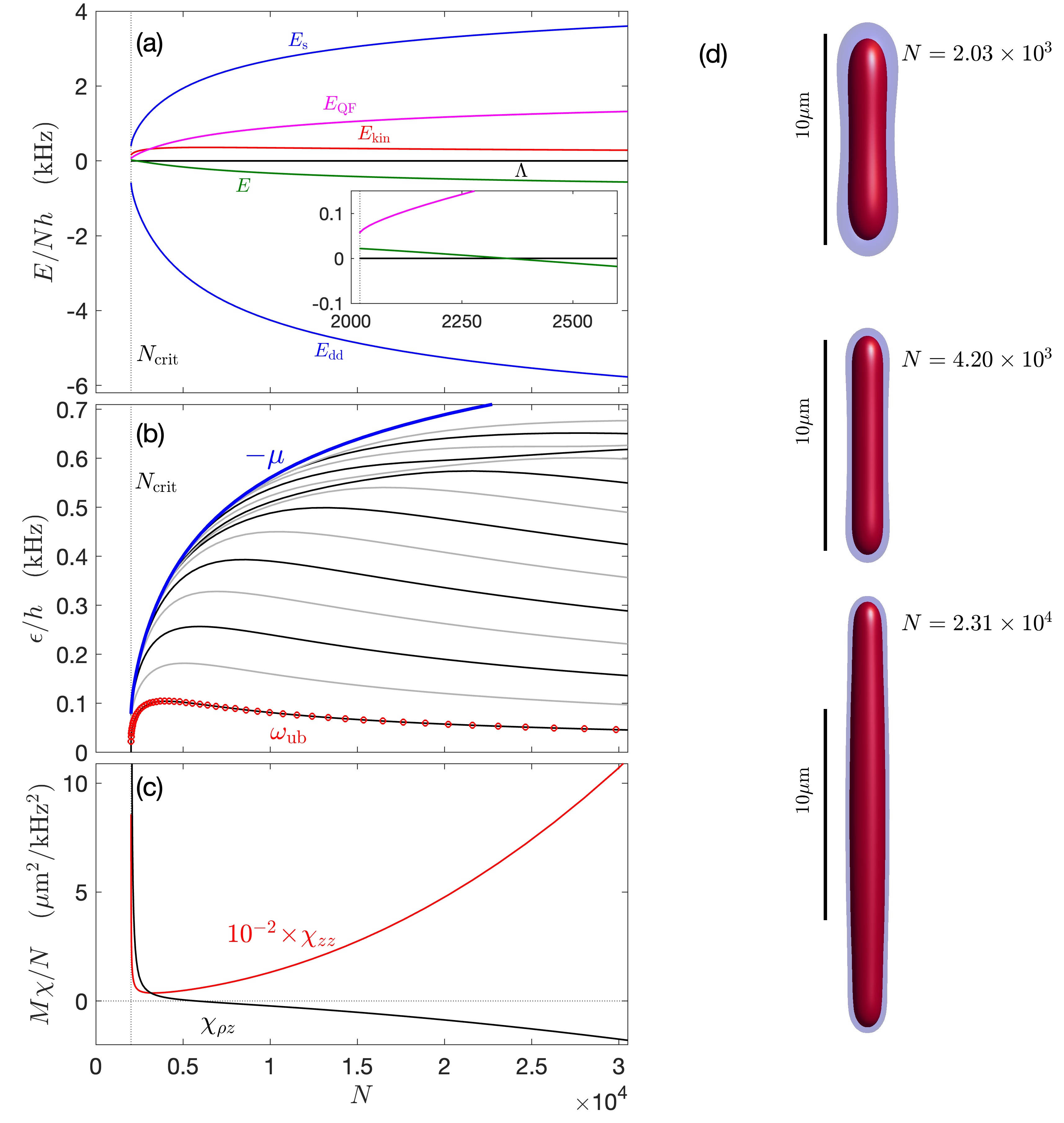
Figure 1: Free-space droplet ($V=0$) as a function of atom number $N$. (a) Components of energy and the virial $\Lambda$. Inset shows a zoom in close to $N_{\mathrm{crit}}\approx 2020$ to reveal where the total energy is positive. (b) Results from numerical solution of the BdG equations for the $m=0$ excitations that are even (black lines) and odd (grey lines) with respect to a reflection along $z$ through the droplet center. The approximate result $\omega_{\text{ub}}$ obtained from (15) (red circles). The droplet binding energy, characterized by $-\mu$, is shown for reference (blue line). (c) The static polarizabilities $\chi_{zz}$ and $\chi_{\rho z}$. Results for ¹⁶⁴Dy using $a_{\mathrm{dd}}=130.8\,a_{0}$ and $a_{s}=80\,a_{0}$. (d) Density isosurfaces of droplet states for various $N$ values as labelled. Isosurfaces shown for $10^{18}\,$m^-3 (blue) and $10^{19}\,$m^-3 (red).

III Results for free-space droplets

III.1 Energetics

In Fig. 1 we consider a free-space (self-bound) ¹⁶⁴Dy droplet for $a_{s}=80\,a_{0}$ (i.e. $\epsilon_{\mathrm{dd}}=1.64$) as a function of $N$. For $N>N_{\mathrm{crit}}\approx 2020$ a self-bound droplet solution exists, while for $N<N_{\mathrm{crit}}$ there is no droplet solution, and the atoms expand to fill all space. In Fig. 1(a) we examine the energy of the free-space droplet, seeing that as $N$ approaches $N_{\mathrm{crit}}$ from above the total energy of the droplet becomes positive (for $N\lesssim 2,350$, see inset). When the energy is positive the droplet is metastable. We show some examples of the droplet states in Fig. 1(c) to give some context on the size and shape of the droplet as $N$ varies.

We also consider the components of energy, defined by

$$E_{\text{kin}} =-\frac{\hbar^{2}}{2M}\int d\mathbf{x}\,\psi^{*}\nabla^{2}\psi,$$ (17)

$$E_{\mathrm{pot}} =\int d\mathbf{x}\,V(\mathbf{x})|\psi|^{2},$$ (18)

$$E_{s} =\frac{1}{2}g_{s}\int d\mathbf{x}\,|\psi|^{4},$$ (19)

$$E_{\mathrm{dd}} =\frac{1}{2}\int d\mathbf{x}\,\Phi_{\mathrm{dd}}(\mathbf{x})|\psi|^{2},$$ (20)

$$E_{\mathrm{QF}} =\frac{2}{5}\gamma_{\mathrm{QF}}\int d\mathbf{x}\,|\psi|^{5}$$ (21)

as the kinetic, potential, contact interaction, DDI, and quantum fluctuation energy, respectively. For this free-space case $E_{\mathrm{pot}}=0$. We observe that the DDI and contact interaction energies are the largest energies by magnitude, but have opposite sign. The quantum fluctuation term is necessary to stabilise the droplet solution against mechanical collapse driven by the interaction terms, but is typically significantly smaller in magnitude than either of the interaction energies. The kinetic energy is smaller than all other components except when $N\to N_{\mathrm{crit}}$, where it can exceed $E_{\mathrm{QF}}$.

A virial relation for the system can be obtained by considering how the energy functional transforms under a scaling of coordinates (e.g. see Dalfovo et al. (1999)). For the dipolar EGPE in a harmonic trap this relation is

$$\Lambda\equiv E_{\text{kin}}-E_{\mathrm{pot}}+\frac{3}{2}(E_{s}+E_{\mathrm{dd}})+\frac{9}{4}E_{\text{QF}}=0,$$ (22)

and provides a connection between the energy components Triay (2019); Lee et al. (2021). In Fig. 1(a) we show $\Lambda$ for reference. This turns out to be a sensitive test of the accuracy of dipolar quantum droplet solutions Lee et al. (2021), and the results we present here typically have $|\Lambda/Nh|\ll 10^{-3}\,$Hz.

III.2 Excitations

In Fig. 1(b) we show the spectrum of $m=0$ modes in the droplet as a function of $N$. Excitations for other $m$ values have been examined in Ref. Baillie et al. (2017). The lowest energy excitation branch for the quantum droplets is $m=0$ (this is not the case for vortex states, e.g. see Lee et al. (2018)). We note that the excitations are measured relative to the condensate chemical potential. Thus excitations with $\hbar\omega_{\nu}>-\mu$ are unbounded by the droplet potential and are part of the continuum. For this reason we only calculate excitations with $\hbar\omega_{\nu}<-\mu$. From these results we observe that the lowest $m=0$ mode goes soft (i.e. approaches zero energy) as $N\to N_{\mathrm{crit}}$. This indicates the onset of a dynamical instability of the self-bound state. We also show the excitation frequency bound $\omega_{\mathrm{ub}}$ obtained from ground state calculations according to Eq. (15). This is seen to be in good agreement with the BdG result for the lowest excitation over the full range of atom numbers considered.

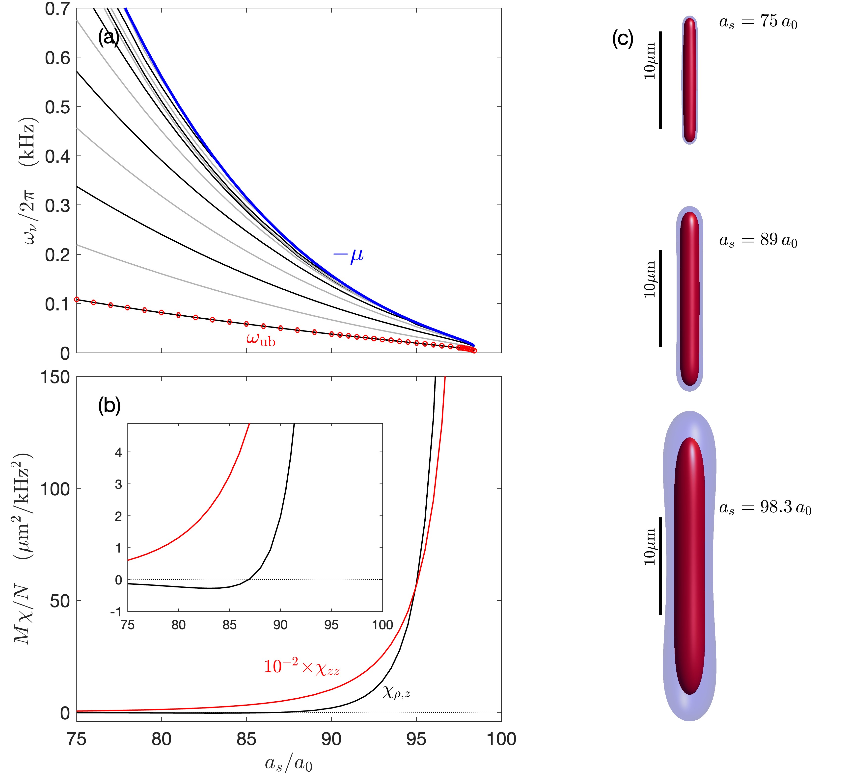
Figure 2: Free-space droplet ($V=0$) as a function of s-wave scattering length $a_{s}$. (a) Results from numerical solution of the BdG equations for the $m=0$ excitations that are even (black lines) and odd (grey lines). The droplet binding energy, characterized by $-\mu$, is shown for reference (blue line). The approximate result $\omega_{\text{ub}}$ obtained from (15) (red circles). The droplet binding energy, characterized by $-\mu$, is shown for reference (blue line). (b) The static polarizabilities $\chi_{zz}$ and $\chi_{\rho z}$. (c) Density isosurfaces of droplet states for various $a_{s}$ values as labelled. Isosurfaces shown for $10^{18}\,$m^-3 (blue) and $10^{19}\,$m^-3 (red). Results for $N=10^{4}$ ¹⁶⁴Dy atoms using $a_{\mathrm{dd}}=130.8\,a_{0}$.

In Fig. 1(c) we show results for the static polarizabilities. The axial result $\chi_{zz}$ [used in Eq. (15)] is always positive, reflecting that the application of a weak axial confinement to the free-space droplet causes it to shorten. The magnitude of $\chi_{zz}$ tends to be much larger than $\chi_{\rho z}$, so we have scaled it by a factor of $10^{-2}$ to make the two polarizabilities easier to compare. The transverse response $\chi_{\rho z}$ changes sign depending on the atom number. In the deeply bound droplet regime (i.e. for $N>5\times 10^{3}$, where $\mu$ is large and negative), it is negative. Thus a weak compression along $z$ results in the droplet expanding transversally. In contrast, closer to the unbinding threshold ($N<5\times 10^{3}$), $\chi_{\rho z}$ is positive, and the transverse width will decrease with axial compression. This occurs as the lowest $m=0$ mode starts to soften. This change in behaviour of the transverse response occurs as the lowest excitation mode changes from quadrupolar character at high $N$ to monopole (compressional) character at low $N$ Baillie et al. (2017).

III.3 Results with varying $a_{s}$

In Fig. 2(a) we show results for the $m=0$ excitations of a free-space droplet with a fixed number $N=10^{4}$, but with $a_{s}$ varying. Here the droplet unbinds at $a_{s}\approx 98.5\,a_{0}$, when the lowest energy mode goes soft. The BdG calculations for the energy of the lowest mode are again seen to be in good agreement with the results of Eq. (15). In Fig. 2(b) we examine the response of the ground state to a change in axial confinement. For the deeply bound droplet ($a_{s}\lesssim 87\,a_{0}$) $\chi_{\rho z}$ is negative, while close to unbinding ($a_{s}\gtrsim 87\,a_{0}$) it becomes positive [see inset to Fig. 2(b)].

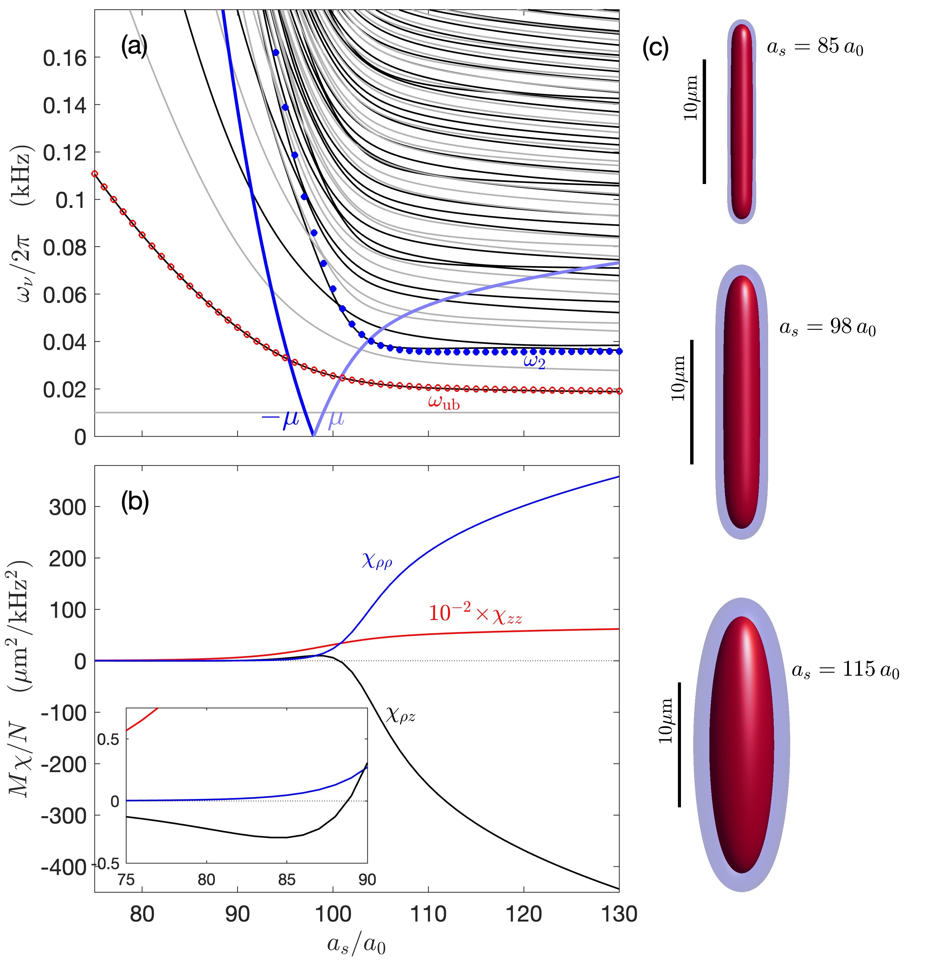
Figure 3: Trapped quantum droplet as a function of s-wave scattering length $a_{s}$. (a) Results from numerical solution of the BdG equations for the $m=0$ excitations that are even (black lines) and odd (grey lines). The approximate result $\omega_{\text{ub}}$ obtained from (15) (red circles) and the excitation frequency estimate $\omega_{2}$ from Eq. (23) (blue circles). The energy scales $\pm\mu$ are shown for reference (blue lines). (b) The static polarizabilities $\chi_{zz}$, $\chi_{\rho z}$ and $\chi_{\rho\rho}$. (c) Density isosurfaces of droplet states for various $a_{s}$ values as labelled. Isosurfaces shown for $10^{18}\,$m^-3 (blue) and $10^{19}\,$m^-3 (red). Results for $N=10^{4}$ ¹⁶⁴Dy atoms using $a_{\mathrm{dd}}=130.8\,a_{0}$ and $(\omega_{x,y},\omega_{z})/2\pi=(20,10)\,$Hz.

IV Results for trapped droplet

In Fig. 3(a) we show the excitation spectrum for a droplet confined in a weak cigar-shaped trap $(\omega_{x,y},\omega_{z})=2\pi\times(20,10)\,$Hz. This geometry allows a smooth crossover between a self-bound droplet and a trap-bound dipolar BEC. Apart from the trap, the parameters of these results are otherwise identical to the case studied in Fig. 2. For $a_{s}\lesssim 95\,a_{0}$ the lowest excitation energies, and chemical potential are similar for the trapped and untrapped cases. A notable feature is the emergence of a Kohn mode at the axial trap frequency $\omega_{z}$. For $a_{s}\gtrsim 95\,a_{0}$ the trap starts playing an increasingly important role. In this regime the droplet self-binding begins to fail and the trap provides the confinement [see Fig. 3(c)]. As this happens the chemical potential becomes positive. Since the trap binds excitations at all energy scales, we show BdG results with $\hbar\omega_{\nu}>-\mu$.

For the full range of parameters considered in Fig. 3(a) Eq. (15) is seen to provide an accurate description of the axial mode. The lower energy Kohn mode has no effect on our sum rule since the symmetry of the that mode does not couple tothe $\sigma_{z}$ operator. In Fig. 3(a) we also present results for the transverse equivalent of Eq. (15), i.e.

$$\omega_{2}\equiv\sqrt{\frac{4N\langle\rho^{2}\rangle}{M\chi_{\rho\rho}}},$$ (23)

where $\delta\langle\sigma_{\rho}\rangle=\lambda\chi_{\rho\rho}$ defines the static polarizability for a transverse perturbation of $-\lambda\sigma_{\rho}$. The frequency estimate of Eq. (23) is in reasonable agreement with the second even mode in the trap-bound region, but ascends to a high frequency in the droplet regime. These results indicate that Eq. (23) is of limited use in the droplet regime.

We show results for the static polarizabilities in Fig. 3(b). In the droplet regime $\chi_{zz}\gg|\chi_{\rho\rho}|,|\chi_{\rho z}|$, while in the trap-bound regime they all become of comparable magnitudes. Interestingly $\chi_{\rho z}$ is positive at intermediate values of $a_{s}$. Correspondingly we find that the axial mode changes character from being a quadrupolar excitation at low $a_{s}$ values, to monopolar at intermediate values, before returning to quadrupolar character at high values of $a_{s}$. Aspects of this behavior has also been described within a variational Gaussian approach Wächtler and Santos (2016b).

V Conclusions

In this work we have presented results for the ground state properties of quantum droplets, their collective excitations and static polarizibility related to a change in confinement. The lowest energy collective mode has been measured in experiments by Chomaz et al. Chomaz et al. (2016), and plays a critical role in the instability of a free-space droplet. We have shown that a simple sum rule approach can accurately predict the frequency of this mode over a wide parameter regime. Our results for the static polarizabilities quantify changes in the widths of the droplet in response to variations in the axial or transverse confinement. We observe that the transverse static polarizability (to an axial confinement change) is negative in deeply-bound droplets and crosses over to being positive in weakly-bound or trap-bound droplets. This change correlates with lowest excitation changing from quadrupolar (incompressible) to monopolar (compressible) character.

References

- Griesmaier et al. (2005) Axel Griesmaier, Jörg Werner, Sven Hensler, Jürgen Stuhler, and Tilman Pfau, “Bose-Einstein condensation of chromium,” Phys. Rev. Lett. 94, 160401 (2005).
- Beaufils et al. (2008) Q. Beaufils, R. Chicireanu, T. Zanon, B. Laburthe-Tolra, E. Maréchal, L. Vernac, J.-C. Keller, and O. Gorceix, “All-optical production of chromium Bose-Einstein condensates,” Phys. Rev. A 77, 061601 (2008).
- Lu et al. (2011) Mingwu Lu, Nathaniel Q. Burdick, Seo Ho Youn, and Benjamin L. Lev, “Strongly dipolar Bose-Einstein condensate of dysprosium,” Phys. Rev. Lett. 107, 190401 (2011).
- Aikawa et al. (2012) K. Aikawa, A. Frisch, M. Mark, S. Baier, A. Rietzler, R. Grimm, and F. Ferlaino, “Bose-Einstein condensation of erbium,” Phys. Rev. Lett. 108, 210401 (2012).
- Lahaye et al. (2009) T Lahaye, C Menotti, L Santos, M Lewenstein, and T Pfau, “The physics of dipolar bosonic quantum gases,” Rep. Prog. Phys. 72, 126401 (2009).
- Chomaz et al. (2022) Lauriane Chomaz, Igor Ferrier-Barbut, Francesca Ferlaino, Bruno Laburthe-Tolra, Benjamin L Lev, and Tilman Pfau, “Dipolar physics: a review of experiments with magnetic quantum gases,” Reports on Progress in Physics 86, 026401 (2022).
- Lee et al. (1957) T. D. Lee, Kerson Huang, and C. N. Yang, “Eigenvalues and eigenfunctions of a Bose system of hard spheres and its low-temperature properties,” Phys. Rev. 106, 1135–1145 (1957).
- Lima and Pelster (2011) Aristeu R. P. Lima and Axel Pelster, “Quantum fluctuations in dipolar Bose gases,” Phys. Rev. A 84, 041604 (2011).
- Lima and Pelster (2012) A. R. P. Lima and A. Pelster, “Beyond mean-field low-lying excitations of dipolar Bose gases,” Phys. Rev. A 86, 063609 (2012).
- Petrov (2015) D. S. Petrov, “Quantum mechanical stabilization of a collapsing Bose-Bose mixture,” Phys. Rev. Lett. 115, 155302 (2015).
- Ferrier-Barbut et al. (2016) Igor Ferrier-Barbut, Holger Kadau, Matthias Schmitt, Matthias Wenzel, and Tilman Pfau, “Observation of quantum droplets in a strongly dipolar Bose gas,” Phys. Rev. Lett. 116, 215301 (2016).
- Wächtler and Santos (2016a) F. Wächtler and L. Santos, “Quantum filaments in dipolar Bose-Einstein condensates,” Phys. Rev. A 93, 061603(R) (2016a).
- Bisset et al. (2016) R. N. Bisset, R. M. Wilson, D. Baillie, and P. B. Blakie, “Ground-state phase diagram of a dipolar condensate with quantum fluctuations,” Phys. Rev. A 94, 033619 (2016).
- Kadau et al. (2016) Holger Kadau, Matthias Schmitt, Matthias Wenzel, Clarissa Wink, Thomas Maier, Igor Ferrier-Barbut, and Tilman Pfau, “Observing the Rosensweig instability of a quantum ferrofluid,” Nature 530, 194–197 (2016).
- Schmitt et al. (2016) Matthias Schmitt, Matthias Wenzel, Fabian Böttcher, Igor Ferrier-Barbut, and Tilman Pfau, “Self-bound droplets of a dilute magnetic quantum liquid,” Nature 539, 259–262 (2016).
- Chomaz et al. (2016) L. Chomaz, S. Baier, D. Petter, M. J. Mark, F. Wächtler, L. Santos, and F. Ferlaino, “Quantum-fluctuation-driven crossover from a dilute Bose-Einstein condensate to a macrodroplet in a dipolar quantum fluid,” Phys. Rev. X 6, 041039 (2016).
- Baillie et al. (2017) D. Baillie, R. M. Wilson, and P. B. Blakie, “Collective excitations of self-bound droplets of a dipolar quantum fluid,” Phys. Rev. Lett. 119, 255302 (2017).
- Pal et al. (2022) Sukla Pal, D. Baillie, and P. B. Blakie, “Infinite dipolar droplet: A simple theory for the macrodroplet regime,” Phys. Rev. A 105, 023308 (2022).
- Wächtler and Santos (2016b) F. Wächtler and L. Santos, “Ground-state properties and elementary excitations of quantum droplets in dipolar Bose-Einstein condensates,” Phys. Rev. A 94, 043618 (2016b).
- Ferrier-Barbut et al. (2018) Igor Ferrier-Barbut, Matthias Wenzel, Fabian Böttcher, Tim Langen, Mathieu Isoard, Sandro Stringari, and Tilman Pfau, “Scissors mode of dipolar quantum droplets of dysprosium atoms,” Phys. Rev. Lett. 120, 160402 (2018).
- Lee et al. (2021) Au-Chen Lee, D. Baillie, and P. B. Blakie, “Numerical calculation of dipolar-quantum-droplet stationary states,” Phys. Rev. Research 3, 013283 (2021).
- Pitaevskii and Stringari (2016) Lev Pitaevskii and Sandro Stringari, Bose-Einstein Condensation and Superfluidity, Vol. 164 (Oxford University Press, 2016).
- Menotti and Stringari (2002) Chiara Menotti and Sandro Stringari, “Collective oscillations of a one-dimensional trapped bose-einstein gas,” Phys. Rev. A 66, 043610 (2002).
- Tanzi et al. (2019) L. Tanzi, S. M. Roccuzzo, E. Lucioni, F. Famà, A. Fioretti, C. Gabbanini, G. Modugno, A. Recati, and S. Stringari, “Supersolid symmetry breaking from compressional oscillations in a dipolar quantum gas,” Nature 574, 382 (2019).
- Dalfovo et al. (1999) Franco Dalfovo, Stefano Giorgini, Lev Pitaevskii, and Sandro Stringari, “Theory of Bose-Einstein condensation in trapped gases,” Rev. Mod. Phys. 71, 463 (1999).
- Triay (2019) Arnaud Triay, “Existence of minimizers in generalized Gross-Pitaevskii theory with the Lee-Huang-Yang correction,” (2019), arXiv:1904.10672 [math-ph] .
- Lee et al. (2018) Au-Chen Lee, D. Baillie, R. N. Bisset, and P. B. Blakie, “Excitations of a vortex line in an elongated dipolar condensate,” Phys. Rev. A 98, 063620 (2018).