Direct tomography of quantum states and processes via weak measurements of Pauli spin operators on an NMR quantum processor

Abstract

In this paper, we present an efficient weak measurement-based scheme for direct quantum state tomography (DQST) and direct quantum process tomography (DQPT), and experimentally implement it on an NMR ensemble quantum information processor without involving any projective measurements. We develop a generalized quantum circuit that enables us to directly measure selected elements of the density matrix and process matrix which characterize unknown quantum states and processes, respectively. This generalized quantum circuit uses the scalar $J$-coupling to control the interaction strength between the system qubits and the metre qubit. We experimentally implement these weak measurement-based DQST and DQPT protocols and use them to accurately characterize several two-qubit quantum states and single-qubit quantum processes. An extra qubit is used as a metre qubit to implement the DQST protocol, while for the DQPT protocol, two extra qubits (one as a metre qubit and the other as an ancilla qubit) are used.

I Introduction

In recent decades, the concepts of weak measurements and weak values have attracted immense attention in quantum information processing from the fundamental as well as the applications point of view Yokota et al. (2009); Piacentini et al. (2016a). The weak value of a given observable obtained via a weak measurement, although is in general a complex number, has been shown to carry information about the system at times between pre and post-selction Aharonov and Vaidman (1990); Aharonov et al. (1988). Weak measurements allow us to sequentially measure incompatible observables so as to gain useful information from the quantum system and learn about the initial state without fully collapsing the state Piacentini et al. (2016b). This is in complete contrast to conventional projective measurements, wherein the system collapses into one of the eigenstates resulting in maximum state disturbance Thekkadath et al. (2016). This feature of weak measurements provides an elegant way to address several important issues in quantum theory including the reality of the wave functionLundeen et al. (2011); Bhati and Arvind (2022), observation of a quantum Cheshire Cat in a matter-wave interferometer experimentDenkmayr et al. (2014), observing single photon trajectories in a two-slit interferometerKocsis et al. (2011), and the Leggett-Garg inequalityGroen et al. (2013). Weak measurements are also actively exploited in the field of quantum information processing covering a wide range of applications including quantum state and process tomographyLundeen and Bamber (2012); Bolduc et al. (2016), state protection against decoherenceKim et al. (2012); Wang et al. (2014), quantum state manipulationBlok et al. (2014), performing minimum disturbance measurementsBaek et al. (2008), precision measurements and quantum metrologyZhang et al. (2015), sequential measurement of two non-commuting observablesAvella et al. (2017) and tracking the precession of single nuclear spins using weak measurementsCujia et al. (2019).

Several techniques have focused on direct estimation of quantum states and processes including a method based on phase-shifting technique Feng et al. (2021); Li et al. (2022) and direct measurement of quantum states without using extra auxiliary states or post-selection processes Wang et al. (2022). A selective QPT protocol based on quantum 2-design states was used to perform DQPT Perito et al. (2018) and experimentally demonstrated on different physical platformsSchmiegelow et al. (2011); Gaikwad et al. (2018, 2022a). Conventional QST and QPT methods require a full reconstruction of the density matrix and are computationally resource intensive. On the other hand, weak measurement based tomography techniques have been used to perform state tomography and it was shown that for certain special cases they outperform projective measurements Das and Arvind (2014); Xu et al. (2021). An efficient DQST scheme was proposed which directly measured arbitrary density matrix elements using only a single strong or weak measurement Ren et al. (2019). Circuit-based weak measurement with post-selection has been reported on NMR ensemble quantum information processor Lu et al. (2014).

In this work, we propose an experimentally efficient scheme to perform direct QST and QPT using weak measurements of Pauli spin operators on an NMR ensemble quantum information processor. The scheme allows us to compute desired elements of the density matrix and is designed in such a way that it does not require any ancillary qubits and has reduced complexity as compared to recently proposed weak measurement-based DQST and DQPT methods Kim et al. (2018); Zhang et al. (2017). Our scheme has three major advantages, namely, (i) it does not require sequential weak measurements, (ii) it does not involve implementation of complicated error-prone quantum gates such as a multi-qubit, multi-control phase gate and (iii) it does not require projective measurements. Furthermore, our proposed method is experimentally feasible as it requires a single experiment to determine multiple selective elements of the density/process matrix. Our scheme is general and can be applied to any circuit-based implementation. We experimentally implemented the scheme to characterize several two-qubit quantum states and single-qubit quantum processes with high fidelity. Further, we fed the weak measurement experimental results as input into a convex optimization algorithm to reconstruct the underlying valid states and processesGaikwad et al. (2021). We compared the experimentally obtained state and process fidelities with theoretical predictions and with numerical simulations and obtained a good match within experimental uncertainties.

This paper is organized as follows: A brief review of weak measurements and the detailed schemes for DQST and DQPT are presented in Section II. The details of the experimental implementation of DQST and DQT via weak measurements are given in Section III. Section III.1 describes how to use an NMR quantum processor to perform weak measurements of Pauli spin operators, while Sections III.2 and III.3 contain details of a weak measurement of the Pauli operator $\sigma_{1z}$ and the results of DQST and DQPT performed using weak measurements, respectively. Section IV contains a few concluding remarks.

II General scheme for direct QST and QPT via weak measurements

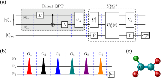
Figure 1: (Color online) (a) General quantum circuit for DQST of an initial unknown state $|\psi\rangle_{s}$ and DQPT of a quantum channel $\Lambda$ using weak measurements. The first (gray-shaded) block corresponds to DQPT performed on the initial state $|0\rangle_{a}|0\rangle_{s}|0\rangle_{m}$. The unitary operator $U_{\chi}$ depends on the operator basis in which DQPT is performed. The second (unfilled) block implements the weak interaction between the system qubits and the meter qubit, followed by measurement on the meter qubit. (b) NMR implementation of the quantum circuit given in panel (a). The Gaussian-shaped curves represents GRAPE-optimized pulses ($\rm{G}_{i}$) corresponding to given unitary operations on all three qubits. (c) Structure of the molecule, trifluoroiodoethylene, used to realize the three NMR qubits $\rm{F}_{1}$, $\rm{F}_{2}$ and $\rm{F}_{3}$.

Consider the system and the measuring device initially prepared in a product state $|\psi\rangle|M\rangle$. The weak measurement of an observable ${A}$ requires the evolution of the joint state $|\psi,M\rangle$ under an operator of the form, ${U}_{SM}=e^{-ig{A}\otimes{B}}$, where $g$ is coupling strength ($|g|\ll 1$) between the system and the measuring device. The operator ${B}$ corresponding to the measuring device is chosen such that $\langle M|{B}|M\rangle=0$. In the weak measurement limit ($|g|\ll 1$), the evolution operator can be approximated upto first order in $g$ as, ${U}^{weak}_{SM}=({I}-ig{A}\otimes{B})$ and the evolution of the joint state (system+measuring device) can be worked out as follows Lu et al. (2014):

$$|\psi,M\rangle_{\rm final} = e^{-ig{A}\otimes{B}}|\psi,M\rangle$$ (1)

$$\approx (I-ig{A}\otimes{B})|\psi,M\rangle$$

$$= |\psi,M\rangle-ig{A}|\psi\rangle\otimes{B}|M\rangle$$

We will see that the above equation can be used for QST and QPT by making appropriate measurements on the measuring device.

Generally quantum processes are either represented via the corresponding (i) $\chi$ matrix (also referred to as the process matrix) using a Kraus operator decompositionKraus et al. (1983) or (ii) Choi-Jamiolkowski state using the channel-state duality theorem Jiang et al. (2013). For an $N$-qubit system, the $\chi$ matrix and the Choi-Jamiolkowski state corresponding to quantum channel $\Lambda$ are given by Kraus et al. (1983); Jiang et al. (2013):

$$\Lambda({\rho}_{in}) = \sum_{i=0}^{4^{N}-1}{K}_{i}{\rho}_{in}K_{i}^{\dagger}=\sum_{m,n=0}^{4^{N}-1}\chi_{mn}{E}_{m}\hat{\rho}_{in}{E}_{n}^{\dagger}$$ (2)

$$\left|\Phi_{\Lambda}\right\rangle = (I\otimes\Lambda)|\Phi\rangle=\frac{1}{2^{N/2}}\sum_{m=0}^{2^{N}-1}|m\rangle\otimes\Lambda|m\rangle$$ (3)

where $\chi_{mn}$ in Eq. (2) are elements of the $\chi$ matrix and $|\Phi_{\Lambda}\rangle$ in Eq. (3) is the Choi-Jamiolkowski state; $\{K_{i}\}$’s and the $\{{E}_{i}\}$’s in Eq. (2) are Kraus operators and fixed basis operators respectively, while the quantum state $|\Phi\rangle$ in Eq. (3) is a pure maximally entangled state of $2N$ qubits $|\Phi\rangle=2^{-N/2}\sum_{m=0}^{2^{N}-1}|m\rangle|m\rangle$. The density matrix ${\rho}_{\Lambda}=|\Phi_{\Lambda}\rangle\langle\Phi_{\Lambda}|$ corresponding to the Choi-Jamiolkowski state can be mapped to the $\chi$ matrix using an appropriate unitary transformation $U_{\chi}$ as $\chi=U_{\chi}\rho_{\Lambda}U^{\dagger}_{\chi}$. The unitary transformation matrix $U_{\chi}$ depends only on the fixed set of basis operators $\{E_{i}\}$ (Eq. (2)) and does not depend on the quantum channel to be tomographed. To perform DQPT of a given quantum channel $\Lambda$ in terms of the $\chi$ matrix, we need to apply the unitary transformation $U_{\chi}$ on $|\Phi_{\Lambda}\rangle$ and then follow the direct QST protocol and estimate the desired elements $\chi_{mn}$.

Consider the operators $O^{\phi}_{x}=|\phi\rangle\langle\phi|\otimes\sigma_{x}$ and $O^{\phi}_{y}=|\phi\rangle\langle\phi|\otimes\sigma_{y}$ where $|\phi\rangle$ is a pure system state and $\sigma_{x(y)}$ are single-qubit Pauli spin operators. The expectation values of the $O^{\phi}_{x}$ and $O^{\phi}_{y}$ operators in the weakly evolved joint state (Eq. (1)) turn out to be:

$$\langle O^{\phi}_{x}\rangle = ig\Big{[}\langle\psi|A^{\dagger}|\phi\rangle\langle\phi|\psi\rangle-\langle\phi|A|\psi\rangle\langle\psi|\phi\rangle\Big{]}$$ (4)

$$\langle O^{\phi}_{y}\rangle = -g\Big{[}\langle\psi|A^{\dagger}|\phi\rangle\langle\phi|\psi\rangle+\langle\phi|A|\psi\rangle\langle\psi|\phi\rangle\Big{]}$$ (5)

which can be simplified to:

$$\frac{\langle O^{\phi}_{y}\rangle-i\langle O^{\phi}_{x}\rangle}{-2g}=\langle\phi|A|\psi\rangle\langle\psi|\phi\rangle$$ (6)

Straightforward algebra leads to

$$\frac{\langle O^{\phi}_{y}\rangle-i\langle O^{\phi}_{x}\rangle}{-2g}=\rho_{mn}=\langle m|\rho|n\rangle$$ (7)

Similarly,

$$\frac{\langle O^{\phi}_{y}\rangle-i\langle O^{\phi}_{x}\rangle}{-2g}=\chi_{mn}=\langle m|\chi|n\rangle$$ (8)

Using Eqs. (7) and (8), one can perform direct QST and QPT by measuring $\langle O^{\phi}_{x}\rangle$ and $\langle O^{\phi}_{y}\rangle$ for an appropriate choice of $A$ and $|\phi\rangle$.

It is interesting to note that

$$\langle\phi|A|\psi\rangle\langle\psi|\phi\rangle=\langle A\rangle_{w}^{\phi}\Pi_{\psi}^{\phi}$$ (9)

where $\langle A\rangle_{w}^{\phi}$ is the weak value associated with a post-selection of the system into the state $\phi$ and $\Pi_{\psi}^{\phi}$ is the post-selection probability Thekkadath et al. (2016) We do not use this connection is our work, however, it connects our work with other schemes involving weak values and post-selection.

III NMR implementation of weak measurement scheme

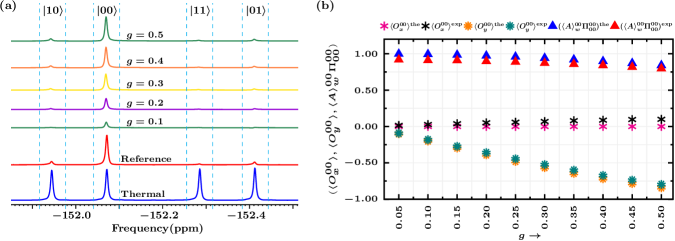
Figure 2: (Color online) (a) NMR spectra obtained by measuring on the third qubit ($\rm F_{3}$), corresponding to the meter qubit. The spectrum in blue represent thermal equilibrium while the spectrum in blue represents the reference spectrum. The other spectra (from top) are obtained by implementing the quantum circuit for weak measurements for different values of $g$, the input state $|00\rangle_{s}|0\rangle_{m}$ and the weak interaction unitary $U^{\rm weak}_{\rm SM}$ corresponding to the Pauli operator $\sigma_{1z}$ followed by a $90^{\circ}$ phase shift on $\rm F_{3}$. (b) The theoretically and experimentally obtained quantities $\langle O^{00}_{x}\rangle,\langle O^{00}_{y}\rangle$ and $\langle A\rangle^{00}_{w}\Pi^{00}_{00}$ are compared for different values of $g$.

III.1 NMR weak measurements of Pauli spin operators

We used the three $\rm{}^{19}F$ spins in the molecule trifluoroiodoethylene dissolved in acetone-D6 to realize three qubits, denoting $\rm F_{1}$ and $\rm F_{2}$ as the system qubits and $\rm F_{3}$ as the meter qubit (Fig. 1(c)). The rotating frame NMR Hamiltonian for a system of three spin-1/2 nuclei is given by Oliveira et al. (2007):

$$\mathcal{H}=-\sum_{i=1}^{3}\nu_{i}I_{iz}+\sum_{i,j=1,i>j}^{3}J_{ij}I_{iz}I_{jz}$$ (10)

where $\nu_{i}$ and $I_{iz}$ are the chemical shift and the $z$-component of the spin angular momentum of the $i$th spin respectively, and $J_{ij}$ is the scalar coupling between the $i$th and $j$th spins. Experimental parameters characterizing the given system can be found in the Reference Gulati et al. (2022).

We set the initial state of the meter qubit to be $|M\rangle=|0\rangle_{m}$, with $B=\sigma_{x}$ (Eq. (1)). In this case, the weak interaction evolution operator ${U}^{weak}_{SM}$ is of the form:

$${U}^{weak}_{SM}={I}-ig{P_{k}}\otimes{\sigma_{x}}$$ (11)

where $I$ is an $8\times 8$ identity matrix and $P_{k}=\{I,\sigma_{x},\sigma_{y},\sigma_{z}\}^{\otimes 2}$ are two-qubit Pauli spin operators. The operator ${U}^{weak}_{SM}$ given in Eq. (11) can be decomposed as:

$$\footnotesize{I}-ig{P_{k}}\otimes{\sigma_{x}} = {I}-ig(U_{k}\sigma_{iz}U_{k}^{\dagger})\otimes(R_{y}(\frac{\pi}{2})\sigma_{z}R_{y}^{\dagger}(\frac{\pi}{2}))$$ (12)

$$= \mathcal{U}_{k}({I}-ig{\sigma_{iz}}\otimes{\sigma_{z}})\mathcal{U}_{k}^{\dagger}$$

where $\sigma_{iz}$ is either $\sigma_{1z}=\sigma_{z}\otimes I$ or $\sigma_{2z}=I\otimes\sigma_{z}$ and $\mathcal{U}_{k}=U_{k}\otimes R_{y}(\frac{\pi}{2})$; $U_{k}$ is a two-qubit unitary operator acting on system qubits and is constructed such that $P_{k}=U_{k}\sigma_{iz}U_{k}^{\dagger}$. To further simplify Eq. (12), consider the $J$-evolution operator $U_{ij}^{J}(t)$:

$$U_{ij}^{J}(t)=e^{-i2\pi J_{ij}I_{iz}I_{jz}t}$$ (13)

If the evolution time $t$ is sufficiently small such that $g=\frac{\pi J_{ij}t}{2}\ll 1$, Eq. (13) can be approximated as:

$$U_{ij}^{J}(t)\approx I-ig\sigma_{iz}\otimes\sigma_{jz}$$ (14)

Hence using Eqs. (12) and (14):

$${U}^{weak}_{SM}\approx\mathcal{U}_{k}U_{ij}^{J}(t)\mathcal{U}_{k}^{\dagger}$$ (15)

where $t=\frac{2g}{\pi J_{ij}}$, $i=1,2$ and $j=3$.

Hence the weak measurement of a desired Pauli operator $P_{k}$ can be performed by applying the sequence of unitary operations given in Eq. (15) on an initial joint state of the three-qubit system followed by the measurement of $O^{\phi}_{x}$ and $O^{\phi}_{y}$. The list of $\mathcal{U}$s corresponding to all $P_{k}$s is given in Table 2.

For the NMR implementation, the quantum circuit depicted in Fig.1(a) is divided into six parts, each consisting of a set of unitary operations. Each of the six parts are implemented using optimized pulse sequences generated through GRAPE, which are represented graphically as colored Gaussian shapes in Fig. 1(b). For example, the first part of the circuit consists of a Hadamard gate followed by a CNOT gate, and this composite operation is implemented using a GRAPE pulse denoted by $\rm{G}_{1}$ in Fig.1(b). The approximate length of the GRAPE optimized rf pulses corresponding to given quantum states (or processes) and Pauli operators is given in Table 1. The power level was set to 28.57 W in all the experiments.

Table 1: Duration of GRAPE pulses (in ms) required to implement the weak measurement based scheme for operators $\sigma_{1z}$, $\sigma_{1x}$, $\sigma_{2x}$ and $\sigma_{1x}\sigma_{2x}$ for a fixed value of $g=0.2$.

	$\sigma_{1z}$	$\sigma_{1x}$	$\sigma_{2x}$	$\sigma_{1x}\sigma_{2x}$
$|\psi_{1}\rangle=(|00\rangle+|11\rangle)/\sqrt{2}$	5.3	5.1	5.2	5.4
$|\psi_{2}\rangle=(|01\rangle+|10\rangle)/\sqrt{2}$	5.3	5.2	5.3	5.6
$\Lambda_{1}=H$	2	0.5	1	1
$\Lambda_{2}=R_{x}(\frac{\pi}{2})$	0.3	2.3	9.5	3.4

Table 2: Unitary operators $\mathcal{U}_{k}$ and $U_{ij}^{J}(t)$ required to implement the weak interaction operation ${U}^{{\rm weak}}_{SM}$ corresponding to all two-qubit Pauli operators $P_{k}$

$P_{k}$	$\mathcal{U}_{k}$	$U_{ij}^{J}(t)$
$\sigma_{2x}$	$Y_{2}$	$U_{23}^{J}(t)$
$\sigma_{2y}$	$\bar{X}_{2}$	$U_{23}^{J}(t)$
$\sigma_{2z}$	$I$	$U_{23}^{J}(t)$
$\sigma_{1x}$	$Y_{1}$	$U_{13}^{J}(t)$
$\sigma_{1x}\sigma_{2x}$	$\bar{Z}_{1}Y_{2}U_{12}^{J}(\frac{1}{2J_{12}})Y_{1}$	$U_{13}^{J}(t)$
$\sigma_{1x}\sigma_{2y}$	$\bar{Z}_{1}\bar{X}_{2}U_{12}^{J}(\frac{1}{2J_{12}})Y_{1}$	$U_{13}^{J}(t)$
$\sigma_{1x}\sigma_{2z}$	$\bar{Z}_{1}U_{12}^{J}(\frac{1}{2J_{12}})Y_{1}$	$U_{13}^{J}(t)$
$\sigma_{1y}$	$\bar{X}_{1}$	$U_{13}^{J}(t)$
$\sigma_{1y}\sigma_{2x}$	$Y_{2}U_{12}^{J}(\frac{1}{2J_{12}})Y_{1}$	$U_{13}^{J}(t)$
$\sigma_{1y}\sigma_{2y}$	$\bar{X}_{2}U_{12}^{J}(\frac{1}{2J_{12}})Y_{1}$	$U_{13}^{J}(t)$
$\sigma_{1y}\sigma_{2z}$	$U_{12}^{J}(\frac{1}{2J_{12}})Y_{1}$	$U_{13}^{J}(t)$
$\sigma_{1z}$	$I$	$U_{13}^{J}(t)$
$\sigma_{1z}\sigma_{2x}$	$X_{1}Y_{2}U_{12}^{J}(\frac{1}{2J_{12}})Y_{1}$	$U_{13}^{J}(t)$
$\sigma_{1z}\sigma_{2y}$	$X_{1}\bar{X}_{2}U_{12}^{J}(\frac{1}{2J_{12}})Y_{1}$	$U_{13}^{J}(t)$
$\sigma_{1z}\sigma_{2z}$	$X_{1}U_{12}^{J}(\frac{1}{2J_{12}})Y_{1}$	$U_{13}^{J}(t)$

NMR Measurement of $O_{x}^{\phi}$ and $O_{y}^{\phi}$

For simplicity, consider the post-selected state $|\phi\rangle$ to be one of the computational basis vectors: $\{|00\rangle,|01\rangle,|10\rangle,|11\rangle\}$ which are required to perform DQST or DQPT (Eq. (17)). In this case, it turns out that the observables $O_{x(y)}^{\phi}$ can be directly measured by acquiring the NMR signal from $\rm F_{3}$ (the meter qubit). The NMR signal of $\rm F_{3}$ consists of four spectral peaks (see thermal spectra in blue color in Fig. 2(a)) corresponding to four transitions associated with density matrix elements (referred to as readout elements): $\rho_{56}$, $\rho_{12}$, $\rho_{78}$ and $\rho_{34}$ Gaikwad et al. (2022b). The first peak from the left in Fig.2(a) corresponds to the post-selected state $|\phi\rangle=|10\rangle$ while the second, third and fourth peaks correspond to the post-selected states $|00\rangle$, $|11\rangle$ and $|01\rangle$, respectively. These peaks (from the left) are also associated with readout elements $\rho_{56}$, $\rho_{12}$, $\rho_{78}$ and $\rho_{34}$, respectively. The line intensity of the absorption mode spectrum ($x$-magnetization) is proportional to the real part of the corresponding readout element of the density matrix while the dispersion mode spectrum ($y$-magnetization) is proportional to the imaginary part of the corresponding readout element:

$$\langle O_{x}^{\phi}\rangle\propto{\rm Re}(\rho_{ij})\quad{\rm and}\quad\langle O_{y}^{\phi}\rangle\propto{\rm Im}(\rho_{ij})$$ (16)

where $\rho_{ij}$ is the readout element of the three-qubit density matrix on which the observables $O_{x(y)}^{\phi}$ are being measured. The complete list of observables $\langle O_{x(y)}^{\phi}\rangle$ with corresponding spectral transitions and readout elements are listed in Table 3. Note that in the case of an arbitrary post-selected state $|\phi\rangle$, one has to decompose the observables $O_{x(y)}^{\phi}$ into Pauli basis operators as $O_{x(y)}^{\phi}=\sum_{i}a_{i}^{x(y)}P_{i}$, then measure $\langle P_{i}\rangle$ corresponding to non-zero coefficients $a_{i}^{x(y)}$ and finally compute $\langle O_{x(y)}^{\phi}\rangle$ for the given $|\phi\rangle$. An efficient way of measuring the expectation value of any Pauli observable is described in Reference Singh et al. (2018).

Table 3: Expectation values $\langle O_{x(y)}^{\phi}\rangle$ corresponding to spectral transitions and readout elements for the post-selected state $|\phi\rangle$ (which is one of the computation basis vectors)

$\langle O_{x(y)}^{\phi}\rangle$	Transitions	elements	Peak (from left)
$\langle O_{x(y)}^{00}\rangle$	$|000\rangle\leftrightarrow|001\rangle$	$\rho_{12}$	second
$\langle O_{x(y)}^{01}\rangle$	$|010\rangle\leftrightarrow|011\rangle$	$\rho_{34}$	fourth
$\langle O_{x(y)}^{10}\rangle$	$|100\rangle\leftrightarrow|101\rangle$	$\rho_{56}$	first
$\langle O_{x(y)}^{11}\rangle$	$|110\rangle\leftrightarrow|111\rangle$	$\rho_{78}$	third

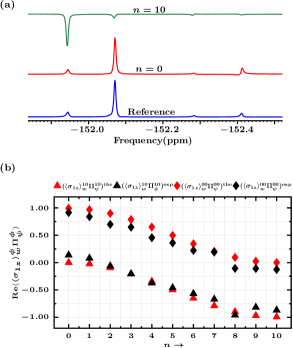
Figure 3: (Color online) (a) NMR spectra obtained after implementing the quantum circuit for weak measurements on the initial state $|\psi\rangle_{s}=\cos{(\frac{n\pi}{20})}|00\rangle+\sin{(\frac{n\pi}{20})}|10\rangle$ for $g=0.1$ and the observable $\sigma_{1z}$. The spectra in green and red correspond to $n=10$ and $n=0$, respectively. (b) Plots comparing the experimentally measured $\langle\sigma_{1z}\rangle_{w}^{\phi}\Pi_{\psi}^{\phi}$ with its theoretical value as a function of the initial state $|\psi\rangle_{s}=\cos{(\frac{n\pi}{20})}|00\rangle+\sin{(\frac{n\pi}{20})}|10\rangle$.

III.2 Experimental weak measurement of $\sigma_{1z}$

As an illustration, we experimentally obtained various relevant quantities (as described in Section II) for the two-qubit Pauli operator $\sigma_{z}\otimes I_{2\times 2}=\sigma_{1z}$. The weak measurement of $\sigma_{1z}$ allows us to measure all the diagonal elements of the density matrix in a single experiment. We experimentally implemented the proposed scheme and measured $\langle O_{x(y)}^{\phi}\rangle$ and $A_{w}^{\phi}\Pi_{\psi}^{\phi}$ with varying weak interaction strength $g$ for the case of $A=P_{k}=\sigma_{1z}$, with the initial state $|\psi\rangle=|00\rangle$ and $|\phi\rangle$ being the computational basis vectors. All the NMR spectrums in Fig.2(a) correspond to measurements on the $\rm F_{3}$ qubit. The bottom spectrum in blue represents the thermal equilibrium spectrum obtained by applying a readout pulse on thermal state followed by detection on the $\rm F_{3}$ qubit. As shown in Table.3, the first peak (from the left) in the thermal spectrum corresponds to $\langle O_{x(y)}^{10}\rangle$, while the second, third and fourth peaks correspond to $\langle O_{x(y)}^{00}\rangle$, $\langle O_{x(y)}^{11}\rangle$ and $\langle O_{x(y)}^{01}\rangle$, respectively.

The reference spectrum depicted in red is obtained by applying a readout pulse on an experimentally prepared pseudo pure state (PPS) using the spatial averaging techniqueOliveira et al. (2007); Cory et al. (1998) followed by detection on the $\rm F_{3}$ qubit. The value of the reference peak is set to be 1. With respect to this reference, the observable $\langle O_{x}^{\phi}\rangle$ can be directly measured by computing spectral intensity by integrating the area under the corresponding peak, while the observable $\langle O_{y}^{\phi}\rangle$ can be measured by first performing a $90^{\circ}$ phase shift and then computing the intensity. Note that the quantity $\langle O_{y}^{\phi}\rangle$ is (-1) times the spectral intensity.

For example, the third spectrum (depicted in green) in Fig.2(a) corresponds to $g=0.1$ The peak intensity with respect to reference spectrum turns out to be $0.1821\pm 0.003$ which gives $\langle O_{y}^{00}\rangle=-0.1821\pm 0.003$ while the experimental value of $\langle O_{x}^{00}\rangle$ (intensity before $90^{\circ}$ phase shift) turns out to be $0.0272\pm 0.0066$. Similarly, the other four spectra in Fig.2(a) correspond to various $g$ values. One can see that from Fig.2(a), the for all values of $g$ the spectral intensity of the first, third and fourth peak corresponding to the post-selected states $|10\rangle$, $|11\rangle$ and $|01\rangle$, respectively, is negligible as compared to the reference peak which implies that the quantities $\langle O_{x(y)}^{10}\rangle$, $\langle O_{x(y)}^{11}\rangle$ and $\langle O_{x(y)}^{01}\rangle$ are almost zero. This is to be expected since theoretically $\langle\phi|\sigma_{1z}|\rho|\phi\rangle=0$ except for $|\phi\rangle=|00\rangle$, whereas the spectral intensity of the second peak corresponding to $\langle O_{y}^{00}\rangle$ is non-zero and increases with $g$.

The experimental values $\langle O_{x(y)}^{00}\rangle$ and ${\langle\sigma_{1z}\rangle}_{w}^{00}\Pi_{00}^{00}$ are compared with their theoretically expected values in Fig. 2(b), for different values of $g$. Only the real part of ${\langle\sigma_{1z}\rangle}_{w}^{00}\Pi_{00}^{00}$, i.e.${\rm Re}({\langle\sigma_{1z}\rangle}_{w}^{00}\Pi_{00}^{00})=\frac{\langle O_{y}^{00}\rangle}{-2g}$ is plotted as the imaginary part turns out to be almost zero (as seen from $\langle O_{x}^{00}\rangle$ values). The experimental quantity ${\langle\sigma_{1z}\rangle}_{w}^{00}\Pi_{00}^{00}$ was calculated using Eq. (LABEL:eq11), however it can also be computed by rescaling the spectrum by the factor $|\frac{1}{2g}|$ with respect to the reference spectrum. The expected value of ${\langle\sigma_{1z}\rangle}_{w}^{00}\Pi_{00}^{00}$ is equal to 1, which is the density matrix element $\rho_{11}$ of initial state $|\psi\rangle=|00\rangle$.

As the value of $g$ increases, the experimental and theoretical value of $\rho_{11}$ deviates more and more from 1, because the weak interaction approximation no longer holds for relatively large values of $g$. At $g=0.05$, the experimental value of $\rho_{11}^{\rm exp}$ was $(0.9198\pm 0.0057)+i(0.0525\pm 0.0399)$, while at $g=0.5$ the value of $\rho_{11}^{\rm exp}$ was $(0.7971\pm 0.0021)+i(0.0989\pm 0.0439)$. We also would like to point out here that in real experiments an arbitrary small value of $g$ may not work, since the signal strength after the weak interaction may be too small to detect and may introduce large errors in the measurements.

We also implemented the weak measurement-based scheme for different initial states. The results shown in Fig.3 were obtained by experimental implementing the weak measurement-based scheme for a fixed interaction strength $g=0.1$ and for different initial states of the form $|\psi\rangle=\cos{(\frac{n\pi}{20})}|00\rangle+\sin{(\frac{n\pi}{20})}|10\rangle$. The NMR spectrum in blue color in Fig.3(a), is the reference spectrum, while the other two spectra in red and green correspond to the states $n=0$ and $n=10$, respectively, which were obtained by implementing the weak measurement quantum circuit (Fig.1) followed by a $90^{\circ}$ phase shift. Note that since the value of $g$ is fixed, the spectra corresponding to all $n$ are rescaled by the factor $\frac{1}{2(0.1)}=5$ with respect to the reference spectrum, which directly yields ${\rm Re}({\langle\sigma_{1z}\rangle}_{w}^{\phi}\Pi_{\psi}^{\phi})$ and ${\rm Im}({\langle\sigma_{1z}\rangle}_{w}^{\phi}\Pi_{\psi}^{\phi})$ (the real and imaginary parts of corresponding density matrix, respectively). For $n=0$ (red spectrum), the observables $\langle O_{y}^{10}\rangle$, $\langle O_{y}^{00}\rangle$, $\langle O_{y}^{11}\rangle$ and $\langle O_{y}^{01}\rangle$ turned out to be $-0.1370\pm 0.0008$, $-0.9137\pm 0.0038$, $-0.0267\pm 0.0010$ and $-0.1243\pm 0.0085$, respectively. For $n=10$ (green spectrum) the observables turned out to be $0.8687\pm 0.0054$, $0.1255\pm 0.0033$, $0.0294\pm 0.0003$ and $0.0237\pm 0.0030$, respectively. The experimentally obtained ${\rm Re}\langle{\sigma_{1z}}_{w}^{\phi}\Pi_{\psi}^{\phi}\rangle$ is compared with the theoretically expected values in Fig. 3(b), for $|\phi\rangle=|00\rangle$ and $|\phi\rangle=|10\rangle$ and for various initial states. The experimental values are in very good agreement with the theoretical predictions in both Figs.2 and 3, which clearly shows the successful implementation of the weak measurement of $\sigma_{1z}$.

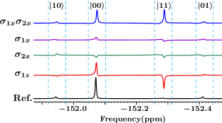
Figure 4: (Color online) Experimental readouts demonstrating DQST of the Bell state $|\psi\rangle_{s}=\frac{1}{\sqrt{2}}(|00\rangle+|11\rangle)$ using weak measurements for a value of $g=0.2$. NMR spectra for the observables $\sigma_{1z}$ (red), $\sigma_{2x}$(green), $\sigma_{1x}$(purple), and $\sigma_{1x}\sigma_{2x}$ (blue) were obtained by implementing the weak measurement quantum circuit, followed by a $90^{\circ}$ phase shift on the initial Bell state.

III.3 Experimental DQST and DQPT using weak measurements

We now proceed to experimentally demonstrate element-wise full reconstruction of the density and process matrices of several states and quantum gates using the proposed weak measurement-based DQST and DQPT schemes. To estimate a desired element $\rho_{mn}$ of the density matrix or $\chi_{mn}$ of the process matrix, one of the possible choices of the post-selected state $|\phi\rangle$, together with the Pauli operator $P_{k}$, is depicted as $(|\phi\rangle,P_{k})$ in the matrix:

$$\footnotesize\begin{pmatrix}(|00\rangle,\sigma_{1z})&(|01\rangle,\sigma_{2x})&(|10\rangle,\sigma_{1x})&(|11\rangle,\sigma_{1x}\sigma_{2x})\\ \rho_{12}^{*}&(|01\rangle,\sigma_{1z})&(|10\rangle,\sigma_{1x}\sigma_{2x})&(|11\rangle,\sigma_{1x})\\ \rho_{13}^{*}&\rho_{23}^{*}&-(|10\rangle,\sigma_{1z})&(|11\rangle,\sigma_{2x})\\ \rho_{14}^{*}&\rho_{24}^{*}&\rho_{34}^{*}&-(|11\rangle,\sigma_{1z})\\ \end{pmatrix}$$ (17)

In this case, the full QST of a two-qubit quantum state requires weak measurements of only four Pauli operators: $\{\sigma_{1z},\sigma_{1x},\sigma_{2x},\sigma_{1x}\sigma_{2x}\}$. The weak measurement of $\sigma_{1z}$ allows us to directly estimate all the diagonal elements representing the populations of the energy eigenstates, while the weak measurements of $\sigma_{1x}$, $\sigma_{2x}$ and $\sigma_{1x}\sigma_{2x}$ yield two off-diagonal elements, each representing a single- and a multiple-quantum coherence.

As an illustration, we experimentally performed DQST of the maximally entangled Bell states: $|\psi_{1}\rangle=(|00\rangle+|11\rangle)/\sqrt{2}$ and $|\psi_{2}\rangle=(|01\rangle+|10\rangle)/\sqrt{2}$ as well as DQPT of two quantum gates: the Hadamard gate $H$ and a rotation gate $R_{x}(\frac{\pi}{2})$. For both DQST and DQPT, the value of $g$ is set to be $0.2$.

Table 4: Experimental state ($|\psi\rangle$) and process($\Lambda$) fidelities obtained using weak measuremet-based DQST and DQPT

State($|\psi\rangle$)/Process($\Lambda$)	$\mathcal{F}(\rho^{{\rm DQST}}_{{\rm weak}})$	$\mathcal{F}(\rho^{{\rm true}}_{{\rm weak}})$
$|\psi_{1}\rangle=(|00\rangle+|11\rangle)/\sqrt{2}$	$0.9511\pm 0.0065$	$0.9791$
$|\psi_{2}\rangle=(|01\rangle+|10\rangle)/\sqrt{2}$	$0.9266\pm 0.0075$	$0.9739$
$\Lambda_{1}=H$	$0.9447\pm 0.0060$	$0.9703$
$\Lambda_{2}=R_{x}(\frac{\pi}{2})$	$0.9476\pm 0.0029$	$0.9729$

The NMR readouts demonstrating the DQST of the Bell state $|\psi_{1}\rangle=(|00\rangle+|11\rangle)/\sqrt{2}$ are shown in Fig. 4, where weak measurements of four Pauli operators were carried out. The NMR readouts corresponding to the weak measurement of $\sigma_{1z}$, $\sigma_{2x}$, $\sigma_{1x}$ and $\sigma_{1x}\sigma_{2x}$ are depicted in red, green, purple and blue respectively, while the spectrum in black represents the reference spectrum. It can be clearly seen that the non-zero spectral intensities of the NMR peaks corresponding to $(|00\rangle,\sigma_{1z})$, $(|11\rangle,\sigma_{1z})$, $(|11\rangle,\sigma_{1x}\sigma_{2x})$ yield the three density matrix elements $\rho_{11}$, $\rho_{44}$ and $\rho_{14}$ respectively, whereas other peak intensities (Eq. (17)) tend to zero as compared to the reference spectrum. The experimentally obtained real and imaginary parts of the density matrix corresponding to the Bell state $|\psi_{1}\rangle$ are given in Eqs. (19)-(20), respectively. All the elements were measured with considerably high accuracy and precision.

It is to be noted that the experimental density matrix is Hermitian by construction (the imaginary part of all diagonal elements can be ignored and set to zero) but may not satisfy positivity and trace conditions as all the independent elements $\{\rho_{ij},i\leq j\}$ are computed individually and independently. For DQST of the Bell state $|\psi_{1}\rangle$, the trace turns out to be $1.3435$ and the eigenvalues are $1.2836$, $0.2825$, $-0.1553$ and $-0.0673$, which do not correspond to a valid density matrix. However, the true quantum state satisfying all the properties of a valid density matrix can be recovered from the experimental density matrix by recasting it as a constrained convex optimization problem Gaikwad et al. (2021):

$$\!\min_{\overrightarrow{\rho}^{\rm true}_{\rm weak}} \|\overrightarrow{\rho}^{\rm true}_{\rm weak}-\overrightarrow{\rho}^{\rm dqst}_{\rm weak}\|_{l_{2}}$$ (18a)

subject to $$\rho^{\rm true}_{\rm weak}\geq 0,$$ (18b)

$${Tr}(\rho^{\rm true}_{\rm weak})=1.$$ (18c)

where ${\rho}^{\rm true}_{\rm weak}$ is the variable density matrix corresponding to the true quantum state to be reconstructed, while ${\rho}^{\rm dqst}_{\rm weak}$ is the experimentally obtained density matrix using the weak measurement-based DQST scheme. The $\rightarrow$ arrow denotes the vectorized form of the corresponding matrix and $\|.\|_{l_{2}}$ represents $l_{2}$ norm, also known as the Euclidean norm of a vector. The valid density matrix ${\rho}^{\rm true}_{\rm weak}$ representing the true quantum state was recovered from ${\rho}^{\rm dqst}_{\rm weak}$ and is given in Eq. (21). We note here in passing that the experimentally obtained density matrices ${\rho}^{\rm dqst}_{\rm weak}$ (or ${\rho}^{\rm true}_{\rm weak}$) corresponding to the states $|\psi_{1}\rangle$ and $|\psi_{2}\rangle$ can be interpreted as the Choi-Jamiolkowski state corresponding to the identity gate ($\Lambda=I$) and the bit flip gate ($\Lambda=\sigma_{x}$), respectively.

$$\rm{Re}(\rho^{\rm dqst}_{\rm weak})=\begin{pmatrix}0.6089\pm 0.0015&-0.0104\pm 0.0007&0.0774\pm 0.0047&0.6314\pm 0.0074\\ -0.0104\pm 0.0007&0.0155\pm 0.0059&0.0633\pm 0.0073&-0.0534\pm 0.0183\\ 0.0774\pm 0.0047&0.0633\pm 0.0073&0.0764\pm 0.0019&-0.0956\pm 0.0292\\ 0.6314\pm 0.0074&-0.0534\pm 0.0183&-0.0956\pm 0.0292&0.6425\pm 0.0011\\ \end{pmatrix}$$ (19)

$$\rm{Im}(\rho^{\rm dqst}_{\rm weak})=\begin{pmatrix}0&-0.0566\pm 0.0085&0.0352\pm 0.0123&0.1126\pm 0.0374\\ 0.0566\pm 0.0085&0&0.0860\pm 0.0217&-0.1384\pm 0.0036\\ -0.0352\pm 0.0123&-0.0860\pm 0.0217&0&0.1367\pm 0.0139\\ -0.1126\pm 0.0374&0.1384\pm 0.0036&0.1367\pm 0.0139&0\\ \end{pmatrix}$$ (20)

$$\rho^{\rm true}_{\rm weak}=\begin{pmatrix}0.4667&-0.0300-0.0333i&-0.0217-0.0618i&0.4858-0.0811i\\ -0.0300+0.0333i&0.0043&0.0058+0.0024i&-0.0255+0.0399i\\ -0.0217+0.0618i&0.0058-0.0024i&0.0092&-0.0118+0.0681i\\ 0.4858+0.0811i&-0.0255-0.0399i&-0.0118-0.0681i&0.5198\\ \end{pmatrix}$$ (21)

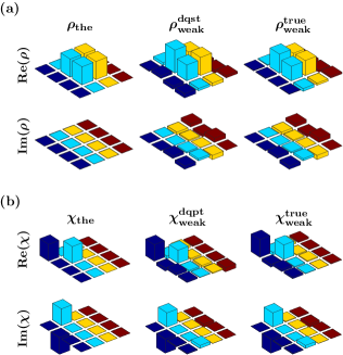
Figure 5: (Color online) Theoretical and experimentally reconstructed density matrices corresponding to (a) the quantum state $|\psi_{2}\rangle=(|01\rangle+|10\rangle)/\sqrt{2}$ and (b) the rotation operation $R_{x}(\frac{\pi}{2})$.

For DQPT implementation, the $U_{\chi}$ acts as a change of basis operation, which transforms the Choi-Jamiolkowski state to the process matrix $\chi$ in the chosen basis. The desired unitary operator $U_{\chi}$ is set to:

$$U_{\chi}=\frac{1}{\sqrt{2}}\begin{pmatrix}1&0&0&1\\ 0&1&1&0\\ 0&-i&i&0\\ 1&0&0&-1\end{pmatrix}$$ (22)

which allows the estimation of the process matrix $\chi$ in the Pauli basis. The real and imaginary parts of the process matrix $\chi^{\rm dqst}_{\rm weak}$ in the Pauli basis corresponding to the Hadamard gate $H$ obtained via the weak measurement-based DQPT protocol are given in Eqs. (23)-(24), respectively, where the trace turned out to be 0.9589 and the eigenvalues are -0.1646, 0.0795, 0.1427 and 0.9014. The true quantum process $\chi^{\rm true}_{\rm weak}$ can be recovered from $\chi^{\rm dqst}_{\rm weak}$ by solving a similar convex optimization problem as given in Eq. (18a) with the additional constraint $\sum_{m,n}\chi_{mn}E_{n}^{\dagger}E_{m}=I$, and is given in Eq. (25). The theoretical process matrix corresponding to the Hadamard gate contains only four non-zero elements $\{\rho_{ij}=0.5|i,j=2,4\}$, and it can be seen from Eqs. (23)-(24) that the weak measuremement scheme is able to determine all these elements with very high accuracy. The theoretical and experimental density and process matrices corresponding to the quantum state $|\psi_{2}\rangle$ and the gate $R_{x}(\frac{\pi}{2})$ are graphically represented in Fig.5. The experimental state (process) fidelity $\mathcal{F}$ is computed using the normalized trace distance between the experimental and theoretical density (process) matricesSingh et al. (2016). The experimental fidelity of various quantum states and processes obtained via the weak measurement-based protocol is given in Table 4.

$$\rm{Re}(\chi^{\rm dqst}_{\rm weak})=\begin{pmatrix}-0.0010\pm 0.0005&0.0422\pm 0.0041&0.0635\pm 0.0012&-0.0854\pm 0.0004\\ 0.0422\pm 0.0041&0.3964\pm 0.0099&-0.0827\pm 0.0004&0.4406\pm 0.0097\\ 0.0635\pm 0.0012&-0.08269\pm 0.0004&0.0789\pm 0.0036&0.0429\pm 0.0019\\ -0.0854\pm 0.0004&0.4406\pm 0.0097&0.0429\pm 0.0019&0.4846\pm 0.0035\\ \end{pmatrix}$$ (23)

$$\rm{Im}(\chi^{\rm dqst}_{\rm weak})=\begin{pmatrix}0&0.0243\pm 0.0033&0.0554\pm 0.0155&-0.0195\pm 0.0012\\ -0.0243\pm 0.0033&0&-0.0664\pm 0.0081&0.0754\pm 0.0445\\ -0.0554\pm 0.0155&0.0664\pm 0.0081&0&0.0633\pm 0.0445\\ 0.0195\pm 0.0012&-0.0754\pm 0.0045&-0.0633\pm 0.0004&0\\ \end{pmatrix}$$ (24)

$$\chi^{\rm true}_{\rm weak}=\begin{pmatrix}0.0319&-0.0145+0.0072i&0.0144+0.0246i&-0.0389+0.0077i\\ -0.0145-0.0072i&0.4021&-0.0380-0.0542i&0.3992+0.0653i\\ 0.0144-0.0246i&-0.0380+0.0542i&0.0831&0.0008+0.0646i\\ -0.0389-0.0077i&0.3992-0.0653i&0.0008-0.0646i&0.4829\\ \end{pmatrix}$$ (25)

Extension to $n$ qubits

For an $n$-qubit density (or process) matrix, all the independent elements $\{\rho_{ij},i\leq j\}$ can be obtained as given in Eq. (17). All the $2^{n}$ diagonal elements can be recovered using a weak measurement of the $\sigma_{1z}=\sigma_{z}\otimes I^{\otimes n-1}$ operator, whereas all the $2^{n-1}(2^{n}-1)$ off-diagonal elements can be obtained via weak measurements of $n$-qubit Pauli operators of the form $\{I,\sigma_{x}\}^{\otimes n}$ (excluding $I^{\otimes n}$), each yielding $2^{n-1}$ elements. For instance, the operator $\sigma_{x}^{\otimes n}$ will measure the off-diagonal elements $\{\rho_{ij},1\leq i\leq 2^{n-1},j=2^{n}+1-i\}$. The reconstruction of the full density matrix requires weak measurements of $2^{n}$ Pauli operators which is in stark contrast to standard tomographic protocols which require the measurement of $4^{n}-1$ operators. Hence, even for full reconstruction, the weak measurement-based tomography protocol turns out to be much more efficient than standard and selective tomography protocols. The quantum circuit given in Fig. 1(a) can be extended to $n$-qubits, with DQST requiring one extra qubit as the meter qubit and DQPT requiring $n$ extra ancillary qubits along the meter qubit.

IV Conclusions

In this work an efficient scheme was proposed and a generalized quantum circuit to perform direct QST and QPT using a weak measurement-based technique was constructed and the protocol was successfully tested on an NMR quantum processor. We used the scalar $J$ coupling to control the strength of the interaction between the system and the metre qubits and hence were able to efficiently simulate the weak measurement process with high accuracy. Our protocol allows us to directly obtain multiple selective elements of the density and the process matrix of an unknown quantum state and an unknown quantum process in a single experiment, which makes it more attractive as compared to other direct tomography methods. Furthermore we employed the convex optimization method to recover the underlying true quantum states and processes from the experimental data sets obtained via the weak measurement-based scheme which substantially improved the experimental fidelities.

Unlike other measurement-based DQST (or DQPT) methods which require projective measurements on the system qubits and maximally disturb the state of the system, our protocol does not involve any measurements on the system qubits. Our experiments open up new research directions for various interesting weak measurement experiments on quantum ensembles which were earlier not possible.