OverlapNetVLAD: A Coarse-to-Fine Framework
for LiDAR-based Place Recognition

Abstract

Place recognition is a challenging yet crucial task in robotics. Existing 3D LiDAR place recognition methods suffer from limited feature representation capability and long search times. To address these challenges, we propose a novel coarse-to-fine framework for 3D LiDAR place recognition that combines Birds’ Eye View (BEV) feature extraction, coarse-grained matching, and fine-grained verification. In the coarse stage, our framework leverages the rich contextual information contained in BEV features to produce global descriptors. Then the top-K most similar candidates are identified via descriptor matching, which is fast but coarse-grained. In the fine stage, our overlap estimation network reuses the corresponding BEV features to predict the overlap region, enabling meticulous and precise matching. Experimental results on the KITTI odometry benchmark demonstrate that our framework achieves leading performance compared to state-of-the-art methods. Our code is available at: https://github.com/fcchit/OverlapNetVLAD.

I INTRODUCTION

Place recognition is a crucial task in mobile robots and autonomous driving, as it enables the recognition of previously visited places and provides a basis for loop closure detection. In particular, it plays a vital role in Simultaneous Localization and Mapping (SLAM), where identifying loop closures helps to correct drift and tracking errors. Visual place recognition (VPR) has been widely studied due to the low cost and rich texture information provided by cameras. In VPR, there are two main methods to describe places: local and global feature descriptors. Local descriptors are selectively extracted from parts of an image with a detection phase, while global descriptors are extracted from the entire image regardless of its content. However, long-term robot operations have revealed that changing appearance is a significant factor in visual place recognition failure[1].

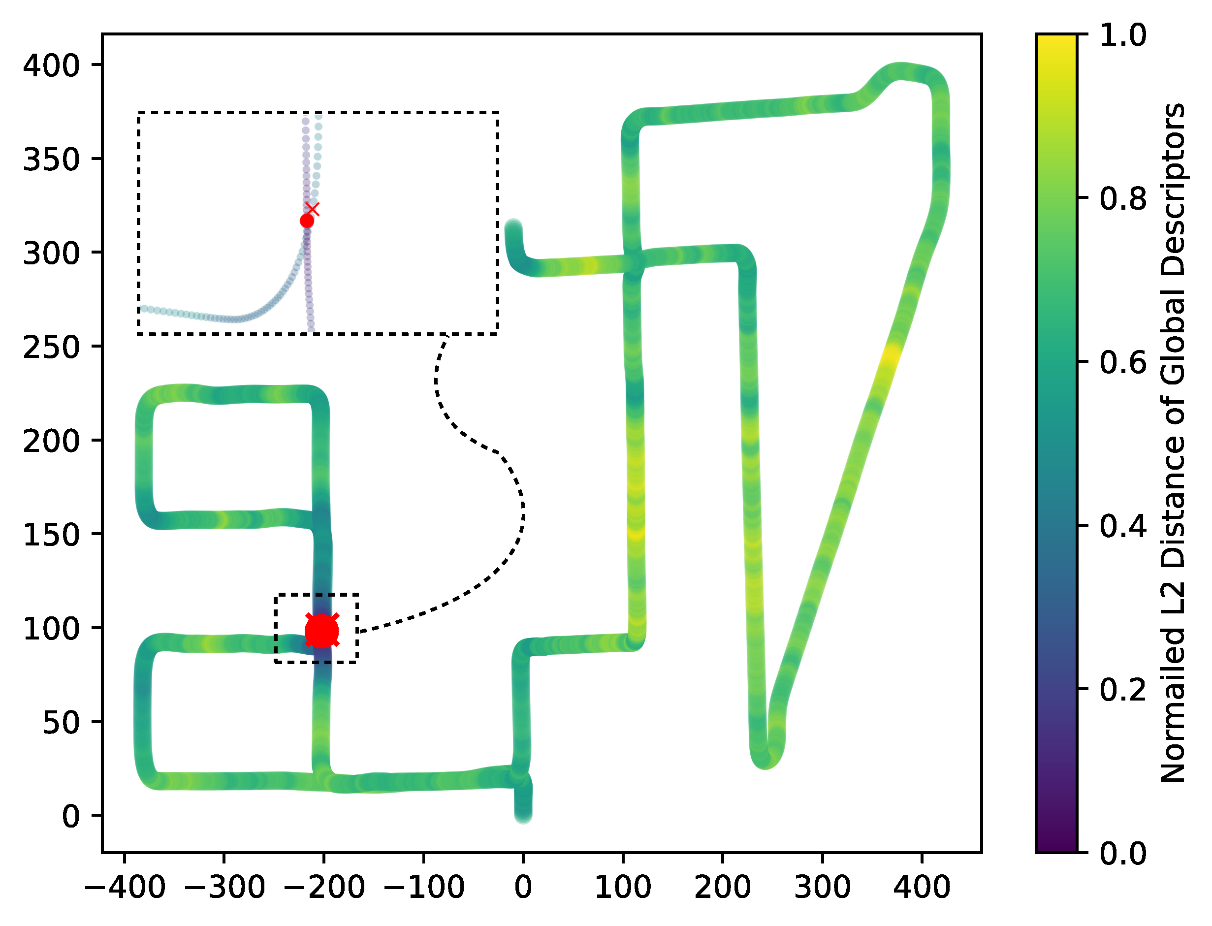
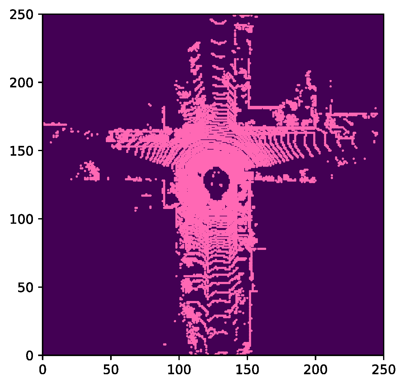
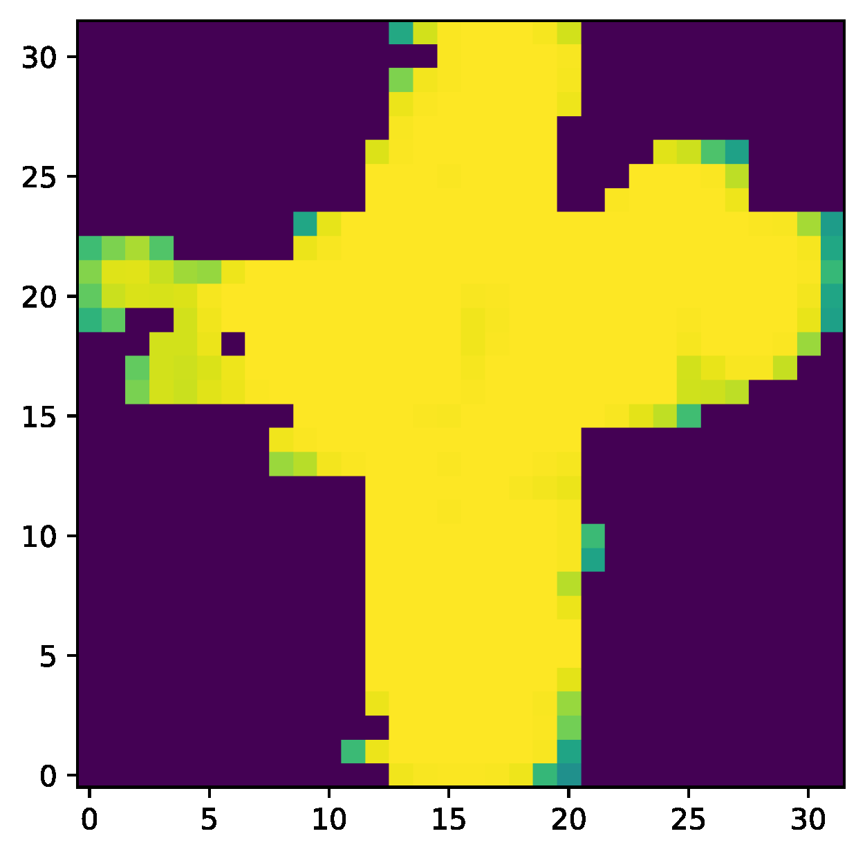
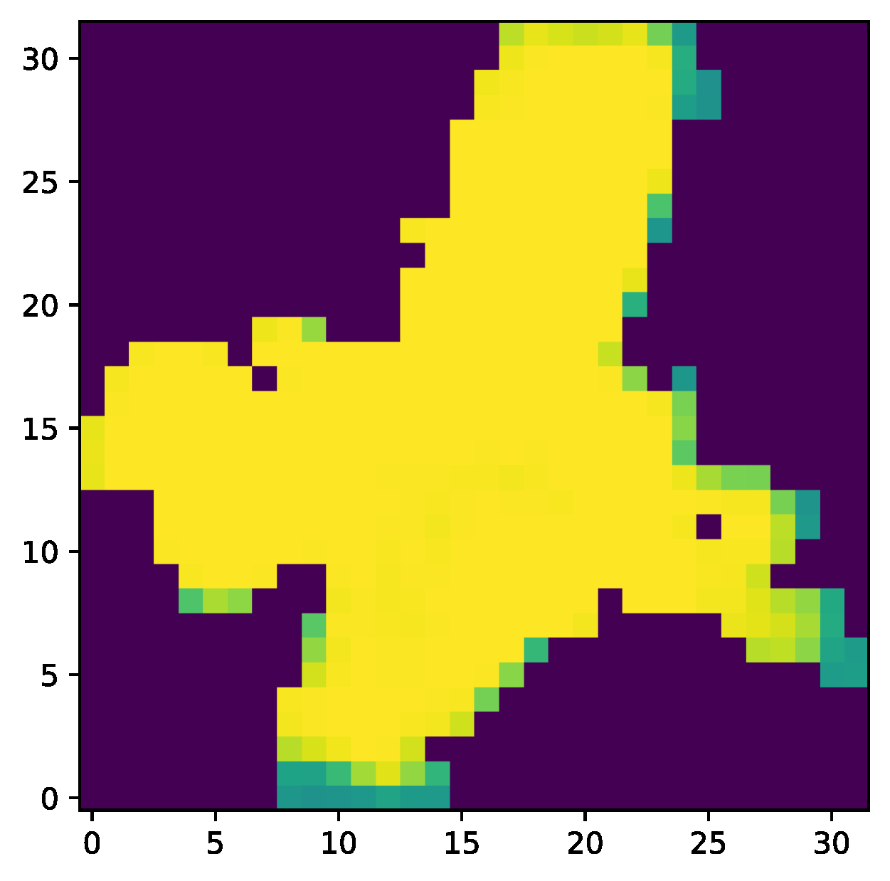
Figure 1: An illustration of our framework. The upper part is the trajectory of sequence 08[2], and the color indicates the normalized Euclidean distance of the descriptors to query one. The circle mark represents a query place, and the cross mark represents the reference place found by our framework. The lower part shows the raw point cloud and overlap prediction (in yellow).

Recently, LiDAR sensors have gained popularity for place recognition due to their ability to provide a wider field of view compared to cameras. Similar to visual place recognition methods, most LiDAR place recognition methods extract features from input point clouds to produce local or global descriptors[3, 4, 5, 6, 7, 8]. However, local descriptors have limited representational power, and the detecting phase is time-consuming, while global descriptors may suffer from overfitting and are less robust to transformations. Inspired by Predator[9], a unified BEV model[10], later called BEVNet, has been proposed to jointly learn 3D local features and overlap estimation. The ability of BEVNet to predict overlap regions significantly enhances its performance on point cloud registration and loop closure. However, the overlap prediction process is time-consuming, and the exhaustive search time increases significantly with the size of the database.

To address these challenges, we propose a novel coarse-to-fine framework based on NetVLAD[11] and BEVNet[10] that efficiently uses BEV features to perform loop closure. Our framework comprises three parts: BEV feature extraction, coarse-grained matching, and fine-grained verification. Since BEV is a well-known natural and straightforward candidate view[12], we first convert the input point cloud to a BEV representation, which is a voxel grid of multiple layers of BEVs. Then the backbone network extracts BEV features in 2D space, which is more efficient than using 3D convolutions due to the sparsity and irregularity of voxels in 3D space. In the coarse-grained matching stage, a global descriptor generation network produces a 1D global descriptor vector from encoded BEV features, and the query scan is matched against all other descriptors in the database to search for the top-K approximate nearest neighbors. Finally, in the fine-grained verification stage, the candidates are further validated by pairwise overlap prediction using an overlap estimation network, and the candidate with the highest overlap score is considered the final match. Our framework is efficient and maintains high place recognition ability. By utilizing the BEV representation, we extract useful information from point clouds and fully utilize it in our place recognition task. The proposed method significantly reduces the time-consuming overlap prediction process and is more effective in determining the matching place than existing methods. Fig.1 provides an illustration of our proposed framework.

The main contributions can be summarized as follows:

• A coarse-to-fine place recognition framework that efficiently uses BEV features to perform loop closure.

• A low-time-consuming coarse place candidate search method based on global descriptor matching.

• An efficient method for validating selected place candidates through overlap detection without prior knowledge.

• Comprehensive experiments and detailed ablation studies on the KITTI dataset[2] to validate the effectiveness of the proposed framework.

II RELATED WORK

II-A Point Cloud Description

To enable comparisons with other point clouds, descriptors are often utilized to provide a distinctive and reliable description of a point cloud feature. Descriptors can be classified into two categories: local descriptors and global descriptors. The difference between them lies in whether they describe the entire point cloud or not.

Local descriptors are usually generated by detecting keypoints. Guo et al.[13] design a local descriptor ISHOT by coupling the geometric and intensity information. Xia et al.[14] propose a self-attention and orientation encoding network called SOE-Net, which incorporates long-range context into point-wise local descriptors. Luo et al.[15] project 3D LiDAR scans to bird’s-eye view images and design a descriptor called bird’s-eye view feature transform (BVFT). However, local descriptors have limited representational power since they only capture local features and cannot capture the global context of the scene. In addition, local descriptors require the detection of feature points in the point cloud and the calculation of the correspondences, resulting in a higher computational cost.

Global descriptors have emerged as an alternative to local descriptors, as they can capture the entire scene and provide a single feature vector for the whole point cloud. Several hand-crafted global descriptors have been proposed, including M2DP [16] and Scan Context [4], which encode the scene into a compact feature representation. Inspired by Scan Context, SSC[5] uses semantic information to improve the representation ability of descriptors.

In recent years, learning-based 3D global descriptors have gained popularity in the research community. PointNetVLAD[3], for example, combines PointNet[17] and NetVLAD[11] to extract global descriptors in an end-to-end manner. SpoxelNet[18] encodes voxelized point clouds into global descriptor vectors, while Locus[19] leverages topological and temporal information and aggregates multi-level features via second-order pooling. Other approaches focus on aggregating semantic information of point clouds. Kong et al.[20] propose a semantic graph representation for place recognition, and Li et al.[7] design a rotation-invariant global descriptor that combines semantic and geometric features and utilize a neural network to predict the similarity of descriptor pairs. There are also methods that explore new ways of encoding the features, such as DiSCO[6] which exploits the magnitude of the spectrum as a place descriptor, and MinkLoc3D[21] which uses a 3D Feature Pyramid Network[22] and GeM[23] pooling to produce global descriptors. FusionVLAD[24] generates multi-view representations from LiDAR scans and uses parallel encoders to fuse top-down and spherical features into translation-insensitive and rotation-invariant global descriptors. More recent works propose novel architectures to improve the representation ability of global descriptors. OverlapTransformer[8] utilizes a yaw-angle-invariant architecture to produce global descriptors using a transformer network, while LoGG3d-Net[25] leverages SparseConv U-Net to extract local feature embeddings, which are aggregated using second-order pooling and Eigen-value Power Normalization to generate global descriptors.

Considering the requirement of the place recognition task, we leverage global descriptors in the coarse searching of our framework. Since NetVLAD exhibits powerful feature representation capabilities and can be easily plugged into any other CNN architecture, we leverage it to generate global descriptors.

II-B Coarse-to-Fine Methods

Coarse-to-fine methods have become increasingly popular in visual place recognition, as they allow for efficient searching of large-scale environments. BoCNF[26] is one such method, which uses BoW in the coarse stage to search for top-K candidate images, followed by a hash-based voting scheme in the fine stage to identify the best match. Similarly, Sarlin et al.[27] propose a hierarchical framework that first performs global retrieval using global descriptors and then matches local features within the candidate places. Qi et al.[28] propose a progressive coarse-to-fine framework that employs global descriptors to discover visually similar references and local descriptors to filter irrelative patterns. They select candidates by global KNN retrieval and then re-rank them by region refinement and Spatial Deviation Index (SDI) spatial verification. Garg et al.[29] propose a semantic-geometric visual place recognition method that also uses the coarse-to-fine matching process for loop closure detection. They design a visual semantics-based descriptor and select the top N matching candidates by a cosine distance-based global place search, followed by keypoint correspondence and spatial layout consistency checks to select the best match. These methods demonstrate the effectiveness of coarse-to-fine strategies in visual place recognition.

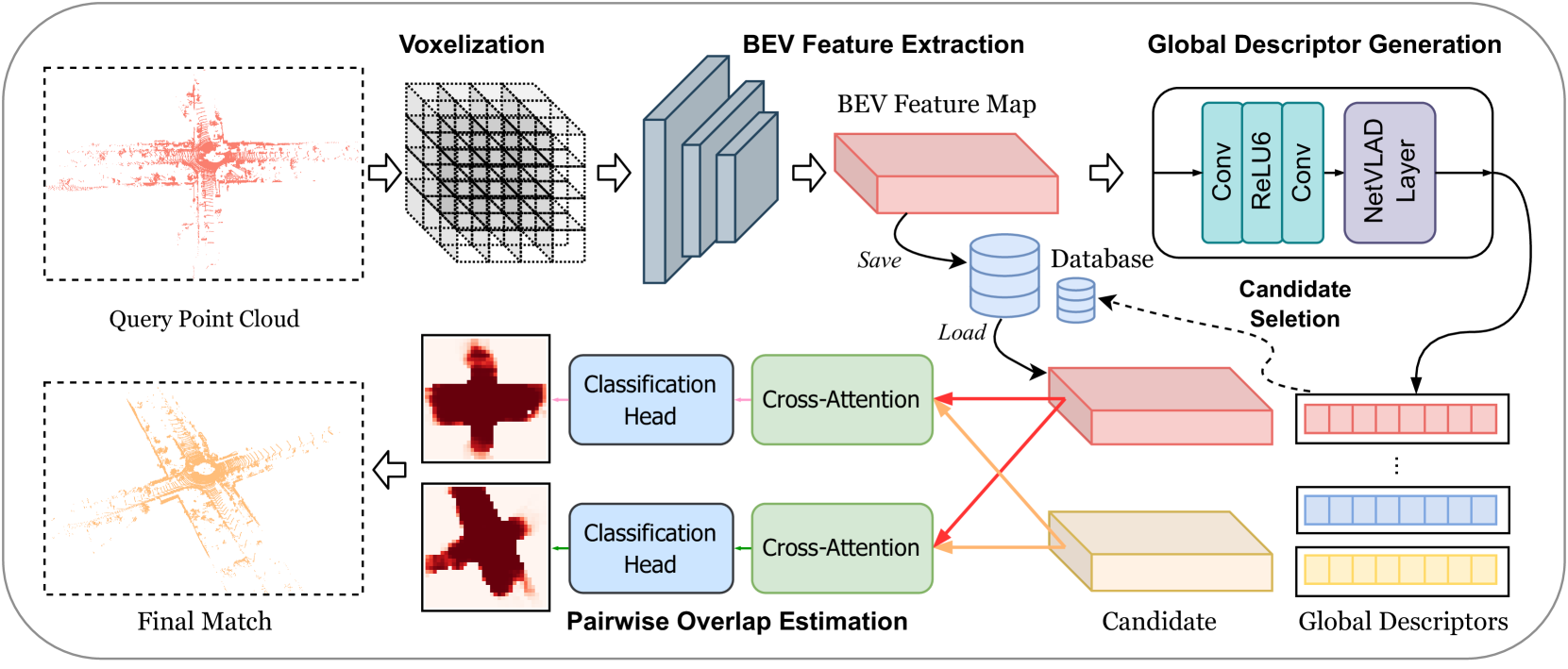
Figure 2: The pipeline of our OverlapNetVLAD. The input point cloud is first converted to a voxel representation, and the encoder network extracts BEV features from the input voxel grid. Then the BEV features are used to generate a global descriptor. In the coarse phase, the descriptor of the query is matched against other descriptors to search for the top-K place candidates. Then in the fine phase, the corresponding BEV features are used to estimate the overlap region between the query scan and the candidates. The best match is selected by similarity score.

In recent years, there has been a growing interest in developing more advanced coarse-to-fine methods for LiDAR-based place recognition. Cop et al.[30] design an intensity-based local descriptor DELIGHT and propose a two-stage framework to perform place recognition. They first search for N most similar DELIGHT descriptors and then perform the geometrical recognition on place candidates. The number N of place candidates is initialed as one and increases during validation until positioning succeeds or fails. Gong et al.[31] propose a two-level framework containing two phases, i.e., description and searching. The searching phase can be seen as a coarse-to-fine method. They first segment the point cloud into multiple clusters and extract the spatial relation descriptors (SRDs) between the clusters to form the spatial relation graph (SRG). They then utilize a two-level matching model to perform a coarse-to-fine matching of the SRGs. The upper-level searching model uses an incremental bag-of-works model to search for candidates. Then The lower-level matching model utilizes an improved spectral method to evaluate the similarities between SRGs.

However, most of the existing methods rely on a single type of descriptor, which may not be able to fully capture the rich geometric information present in the point clouds. This limits their descriptive capability and can lead to a loss of significant information, resulting in unsatisfactory recognition performance. To address these limitations, we propose a novel framework that utilizes a powerful backbone network to extract contextual information for generating global descriptors and predicting overlapping regions. This framework combines the fast but coarse-grained matching of global descriptors with the slow but fine-grained evaluation of overlap regions, allowing for more accurate and efficient place recognition.

III METHODOLOGY

In this section, we describe the details of the proposed coarse-to-fine framework. We begin by introducing the BEV feature extraction process, which uses a backbone network to extract features from the voxel representation of the input point cloud in 2D space. Next, we describe the coarse-grained matching stage, where a global descriptor generation network aggregates the encoded feature map to produce a 1D global descriptor vector, and candidate scans are selected by matching the descriptors. Finally, we introduce the fine-verification stage, where corresponding pairwise BEV features are used to predict overlap regions, and the final match is obtained by calculating the overlap score. We also discuss additional design details, such as loss functions. An overview of our framework is shown in Fig. 2.

III-A BEV Feature Extraction

Since the raw point cloud is irregular and unstructured, we first create a voxel grid from the input point cloud. We adopt a multi-layer occupied BEV representation[6], where each voxel is considered occupied if there is any point in it. By doing this, the point cloud $P$ is divided into a $H_{B}\times W_{B}\times C_{B}$ grid, resulting in a BEV representation $B_{P}\in\mathbb{R}^{H_{B}\times W_{B}\times C_{B}}$.

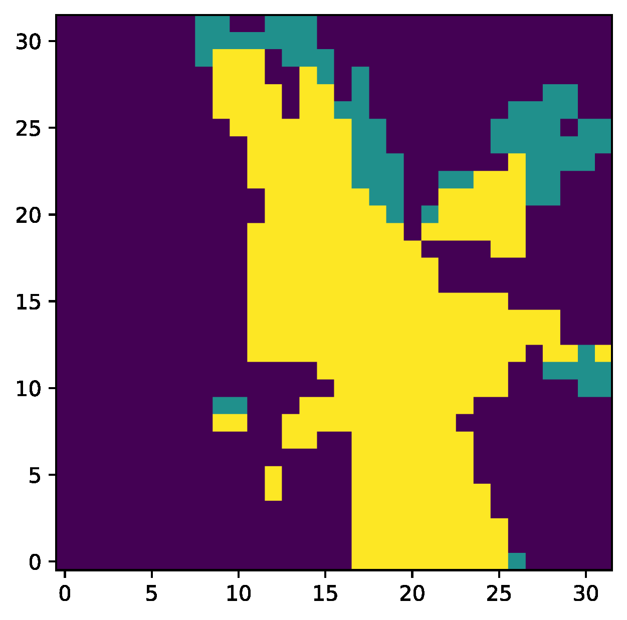
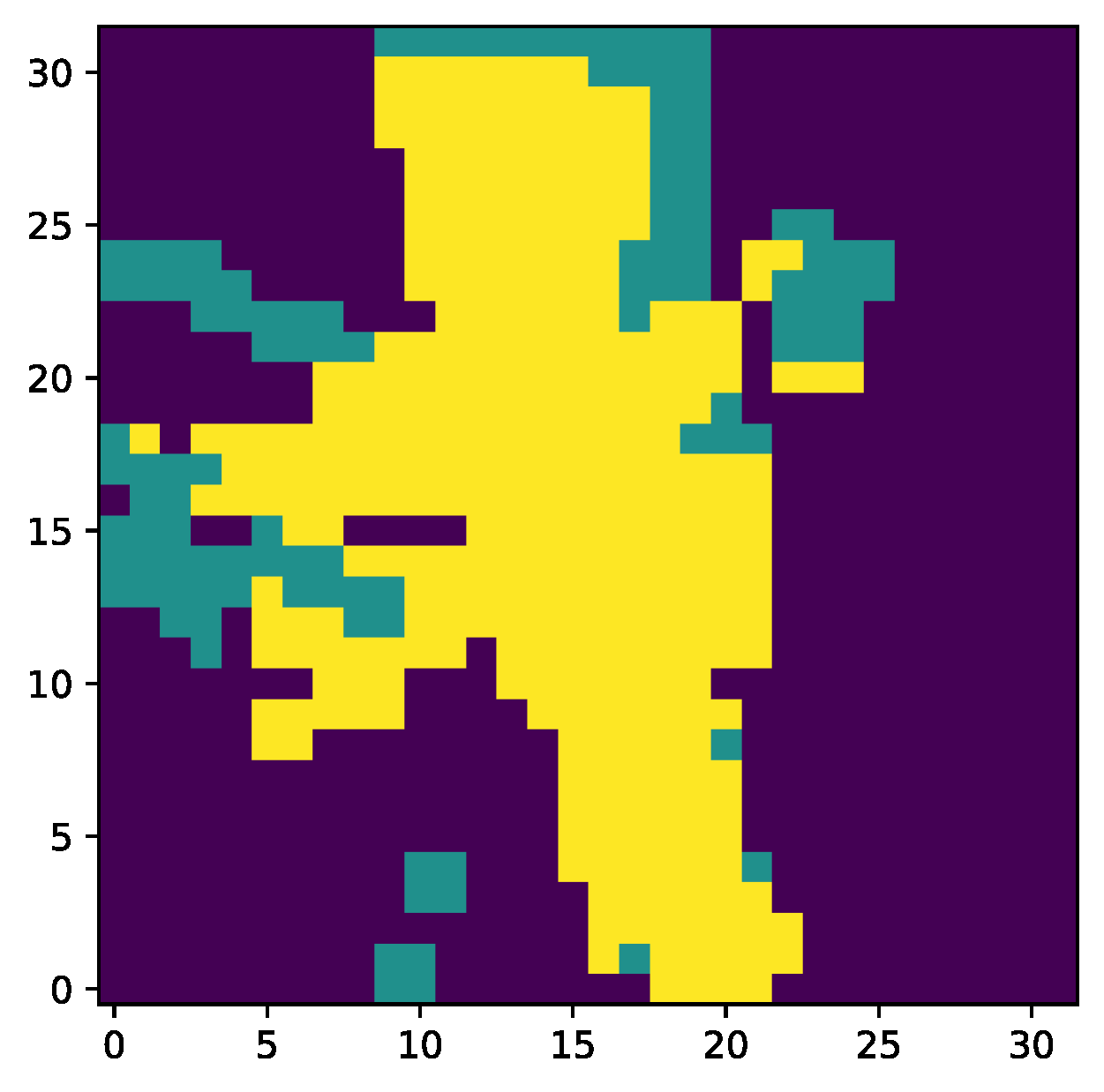
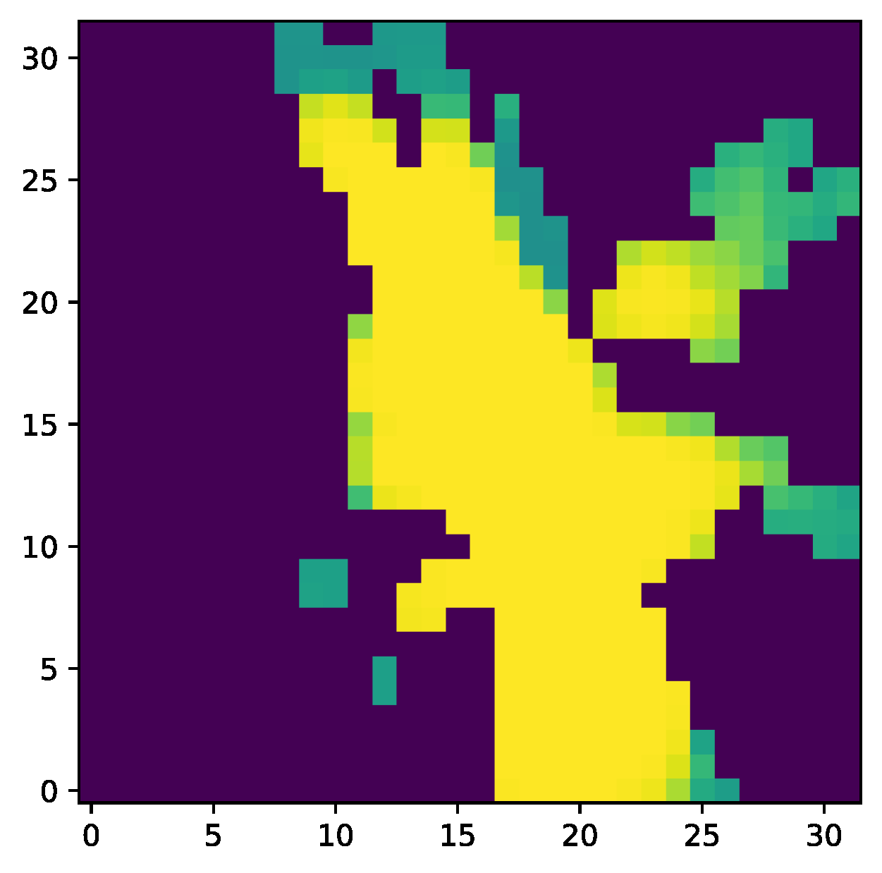
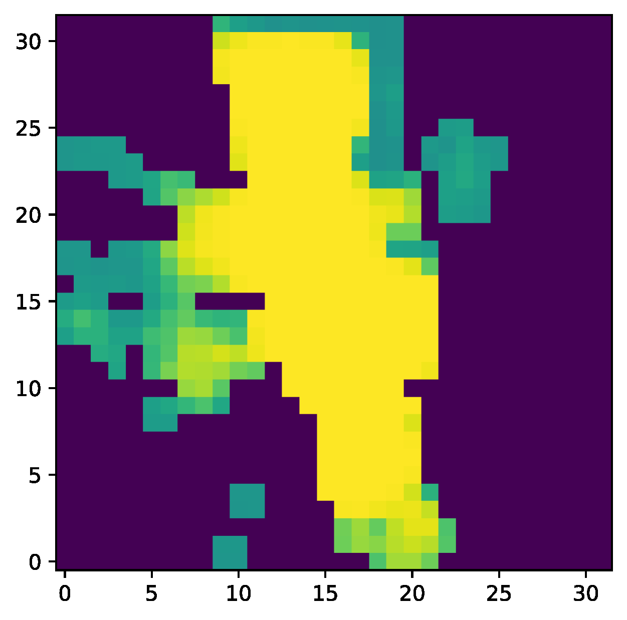
Figure 3: The figure above depicts the process of overlap estimation, where the top row corresponds to the query scan, and the bottom row corresponds to the candidate. Panel (a) shows the voxel grids of the input point clouds. The yellow region in panel (b) represents the ground truth overlap region, and panel (c) shows the predicted overlap region.

Backbone. The encoder module of the BEVNet[10] can effectively extract contextual information, so we leverage it as our backbone network. The backbone is a 2D convolution network with a solid ability to extract complex features. We feed the BEV grid into the network to extract deep features in 2D space. Considering the sparsity of the point cloud, 2D sparse convolutions are used to speed up the feature extraction. The final output feature map (BEV features) contains rich and useful contextual information, which is then stored in the database. The BEV feature map is as follows:

$$E_{P}=\mathcal{E}(B_{P}),$$ (1)

where $\mathcal{E}:B\xrightarrow{}\mathbb{R}^{H_{E}\times W_{E}\times D_{E}}$ is the shared 2D BEV feature extractor, which maps the BEV grid $B_{P}$ to a $H_{E}\times W_{E}\times D_{E}$ dimensional BEV feature map $E_{P}$.

III-B Coarse-Grained Matching

After extracting a BEV feature map from the input voxel grid, the feature $E_{P}$ is passed through the global descriptor generation network. The network comprises two convolutional layers, a NetVLAD layer and a fully connected layer. The last two modules are followed by [3]. First, we leverage the convolutional layers to aggregate features, and the output feature $E^{\prime}_{P}$ is computed as follows:

$$E^{\prime}_{P}=\text{Con}_{3\times 3}(\text{ReLU}(\text{Con}_{3\times 3}(E_{P}))),$$ (2)

then the feature $E^{\prime}_{P}$ is fed into the NetVLAD layer. The NetVLAD layer aggregates local descriptors $\textbf{x}_{i}\in\mathcal{R}^{D}$ within the $(\textit{N}\times D)$-dimension feature by summing the residuals between each descriptor and K cluster centers, which are weighted by soft-assignment of descriptors to multiple clusters. The output VLAD representation V is a $D\times K$ matrix.

$$V(j,k)=\sum_{i=1}^{N}\overline{a}_{k}(\textbf{x}_{i})(x_{i}(j)-c_{k}(j)),$$ (3)

where $\overline{a}_{k}$ denotes the soft-assignment, $\textbf{x}_{i}$ is the $i^{th}$ descriptor in $E^{\prime}_{P}$, and $x_{i}(j)$ is the $j^{th}$ element of the $i^{th}$ descriptor, $c_{k}$ is the $k^{th}$ cluster center.

To reduce computational costs, we utilize a fully connected layer to reduce the dimension of the VLAD descriptors, followed by [3]. Finally, we obtain the global descriptor vector $F(P)\in\mathbb{R}^{\mathcal{O}}$, where $\mathcal{O}\ll(D\times K)$.

The coarse phase of our proposed framework involves searching for candidates close to the query place. Since matching 1D descriptor vectors is computationally efficient, we perform candidate selection by descriptor matching. First, we generate global descriptors for all point clouds and build up a descriptor database. We then compute the distance matrix between the descriptor of the query scan and the remaining descriptors in the database. To select the top-K approximate nearest neighbors as candidate matches, we sort the distances in ascending order based on the K closest distances. However, as the number of descriptors increases significantly with the expansion of the map in real-world autonomous driving scenarios, computation of the distance matrix may become prohibitively slow. To address this, we use a KD-tree implementation to accelerate feature matching. We compute pairwise Euclidean distances between the descriptor vectors of the point clouds $P$ and $Q$.

$$D_{PQ}=\parallel F(P)-F(Q)\parallel_{2},$$ (4)

where $\parallel\cdot\parallel_{2}$ denotes the $L_{2}$ normalization and $F(\cdot)$ denotes the function that maps the input point cloud to a global descriptor vector.

III-C Fine-Grained Verification

In the fine-grained verification stage, we use overlap estimation to identify the most similar place among the top-K candidates. A cross-attention module is utilized to detect the overlap regions. The cross-attention mechanism can effectively interact information[9, 32] and aggregate the contextual information to enhance feature representation. We reuse the previously stored features to reduce the overall computation time. Pairwise BEV features are fed into a cross-attention architecture to fuse features, similar to ImLoveNet[33]. We estimate overlap regions between pairs using the similarity score as an evaluation metric and select the point cloud with the highest overlap score as the final match. The overlap estimation process is illustrated in Fig.3.

Cross-Attention. We use a cross-attention module that is similar to the one used in ImLoveNet [33] but with a slight modification. Instead of fusing deep triple features from 2D images and 3D point clouds, we fuse 2D features $E_{P}$ and $E_{Q}$ to generate relevant feature maps $M_{P}$ and $M_{Q}$.

$$\begin{split}M_{P}&=E_{P}+\text{MLP}(\text{cat}(E_{P},\text{att}(E_{P},E_{Q},E_{Q})))\\ M_{Q}&=E_{Q}+\text{MLP}(\text{cat}(E_{Q},\text{att}(E_{Q},E_{P},E_{P}))),\end{split}$$ (5)

where $\text{MLP}(\cdot)$ denotes a three-layer fully connected network, $\text{cat}(\cdot,\cdot)$ means concatenation and $\text{att}(\cdot,\cdot,\cdot)$ is the attention model.

Classification Head. A binary classification is applied on the correlated feature maps $M_{P}$ and $M_{Q}$ to predict overlap region as follows:

$$\small\gamma_{t}=\text{Sigmoid}(\text{Conv}_{3\times 3}(\text{ReLU}(\text{Conv}_{3\times 3}(M_{t})))),t\in\{P,Q\},$$ (6)

The classification head consists of two $3\times 3$ convolutional layers and a sigmoid layer with ReLU as the activation function.

Overlap Score. The overlap score is used to evaluate the similarity of pairwise point clouds by quantifying the overlapping area. The similarity metric is as follows:

$$\tau=\frac{1}{2}\left(\frac{\sum\gamma_{P}}{V_{P}}+\frac{\sum\gamma_{Q}}{V_{Q}}\right),$$ (7)

where $V_{P}$ and $V_{Q}$ denote the total number of non-zeros volumes of $M_{P}$ and $M_{Q}$.

III-D Loss Function

The training of the descriptor generation network is supervised by quadruplet loss, while the overlap detection network uses classification loss and circle loss[34] as supervisions.

Quadruplet Loss. To train the global descriptor generation network, we use the quadruplet loss $\mathcal{L}_{quad}$. This loss helps the network learn how to accurately describe places so that the descriptors of close places are similar and the descriptors of distant places are significantly different. The quadruplet loss involves four inputs: an anchor, a positive input, and two negative inputs. So our training tuple is as $\mathcal{T}=\left\{F(P_{a}),F(P_{p}),F(P_{n}),F(P_{n}^{*})\right\}$, where $P_{a}$ is an anchor point cloud, $P_{p}$ is a positive point cloud close to $P_{a}$. $P_{n}$ and $P_{n}^{*}$ are two different point clouds far away from $P_{a}$, and these two point clouds are structurally dissimilar to each other as well. The quadruplet loss is as follows:

$$\small\begin{split}\mathcal{L}_{\text{quad}}=&[\|{F(P_{a})-F(P_{p})}\|_{2}-\|{F(P_{a})-F(P_{n})}\|_{2}+\alpha_{1}]_{+}\\ +&[\|{F(P_{a})-F(P_{p})}\|_{2}-\|{F(P_{n})-F(P_{n}^{*})}\|_{2}+\alpha_{2}]_{+},\end{split}$$ (8)

where $[\cdot]_{+}$ is the hinge loss, $\alpha_{1}$ and $\alpha_{2}$ are the constant margins.

Classification Loss. The classification loss adopts a binary cross entropy as

$$\mathcal{L}_{\text{bce}}=\text{BCE}(\gamma_{P},l_{P})+\text{BCE}(\gamma_{Q},l_{Q}),$$ (9)

where $\text{BCE}(\cdot,\cdot)$ represents the binary cross entropy and $l_{P},l_{Q}$ are the ground truth of the overlap.

Circle Loss. In [10], it is found that circle loss can strengthen the network’s ability to perform overlap region classification, so we use circle loss as supervision as well. To balance the distribution of positive and negative samples, random sampling is performed on BEV feature maps. Positive and negative sets of correspondences are then formed for each element $E_{P_{i}}$ of the BEV feature map $E_{P}$. Specifically, the positive set $\Omega_{p}(E_{P_{i}})$ is defined as points in $E_{Q}$ that lie within a radius $r_{p}$ around $E_{P_{i}}$, while the negative set $\Omega_{n}(E_{P_{i}})$ consists of points outside a radius $r_{n}$. The circle loss of $E_{P}$ is formulated as follows:

$$\small\mathcal{L}_{cir}^{P}=\frac{1}{n_{P}}\sum^{n_{P}}_{i=1}log\left[1+\sum_{j\in\Omega_{p}}e^{\beta_{p}^{j}(d_{i}^{j}-\Delta_{p})}\cdot\sum_{k\in\Omega_{n}}e^{\beta_{n}^{k}(\Delta_{n}-d_{i}^{k})}\right],$$ (10)

where $d_{i}^{j}=\|f^{\prime}_{E_{P_{i}}}-f^{\prime}_{E_{Q_{j}}}\|_{2}$ denotes distance in the feature space, and $\Delta_{n}$, $\Delta_{p}$ are negative and positive margins, the weights $\beta_{p}^{j}$ and $\beta_{n}^{k}$ are determined individually for each positive and negative example. The reverse loss $\mathcal{L}_{cir}^{Q}$ is computed in the same way, and the total circle loss $\mathcal{L}_{cir}=\frac{1}{2}(\mathcal{L}_{cir}^{P}+\mathcal{L}_{cir}^{Q})$.

IV EXPERIMENTS

To demonstrate the effectiveness and practicality of our proposed OverlapNetVLAD framework for LiDAR-based place recognition, we designed a series of experiments. Specifically, we evaluate our method on the widely-used KITTI odometry benchmark and compare its performance with other state-of-the-art place recognition methods. Furthermore, we conduct ablation studies to investigate the impact of each module on the final results.

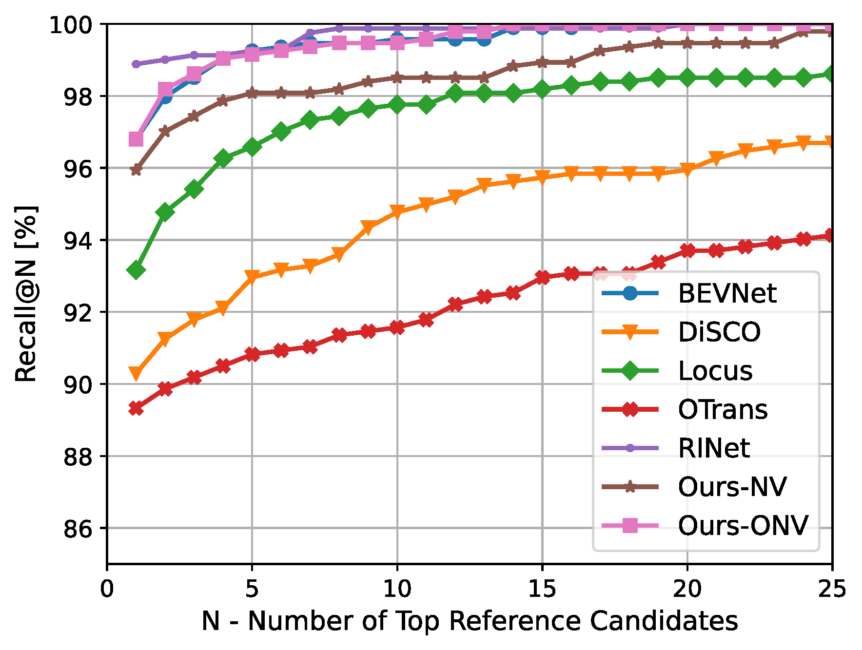
(a) 00

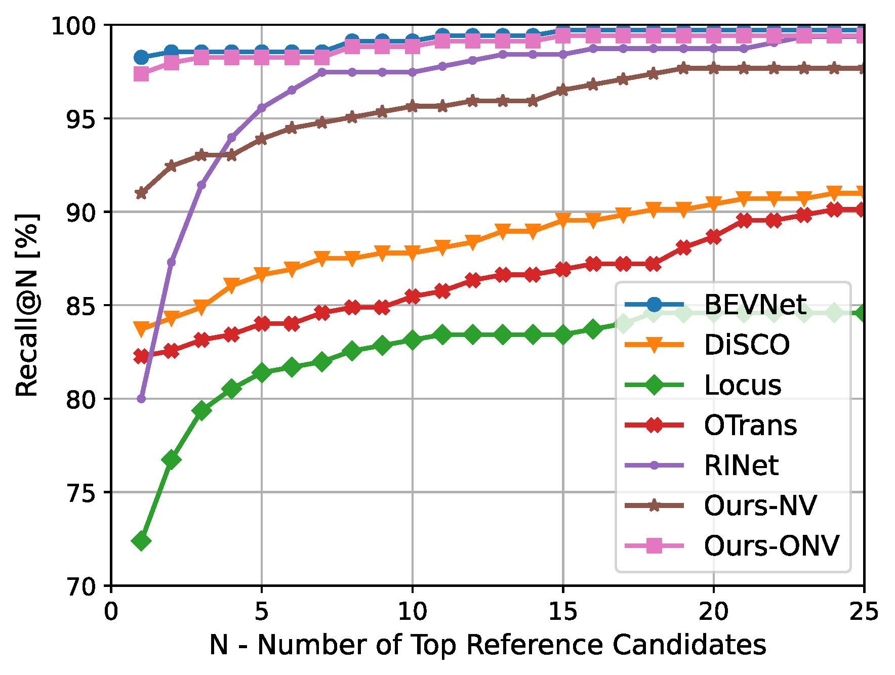
(b) 02

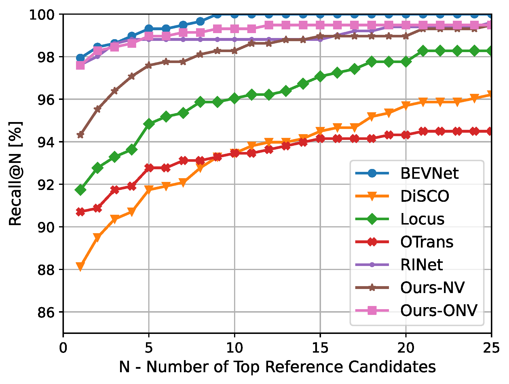
(c) 05

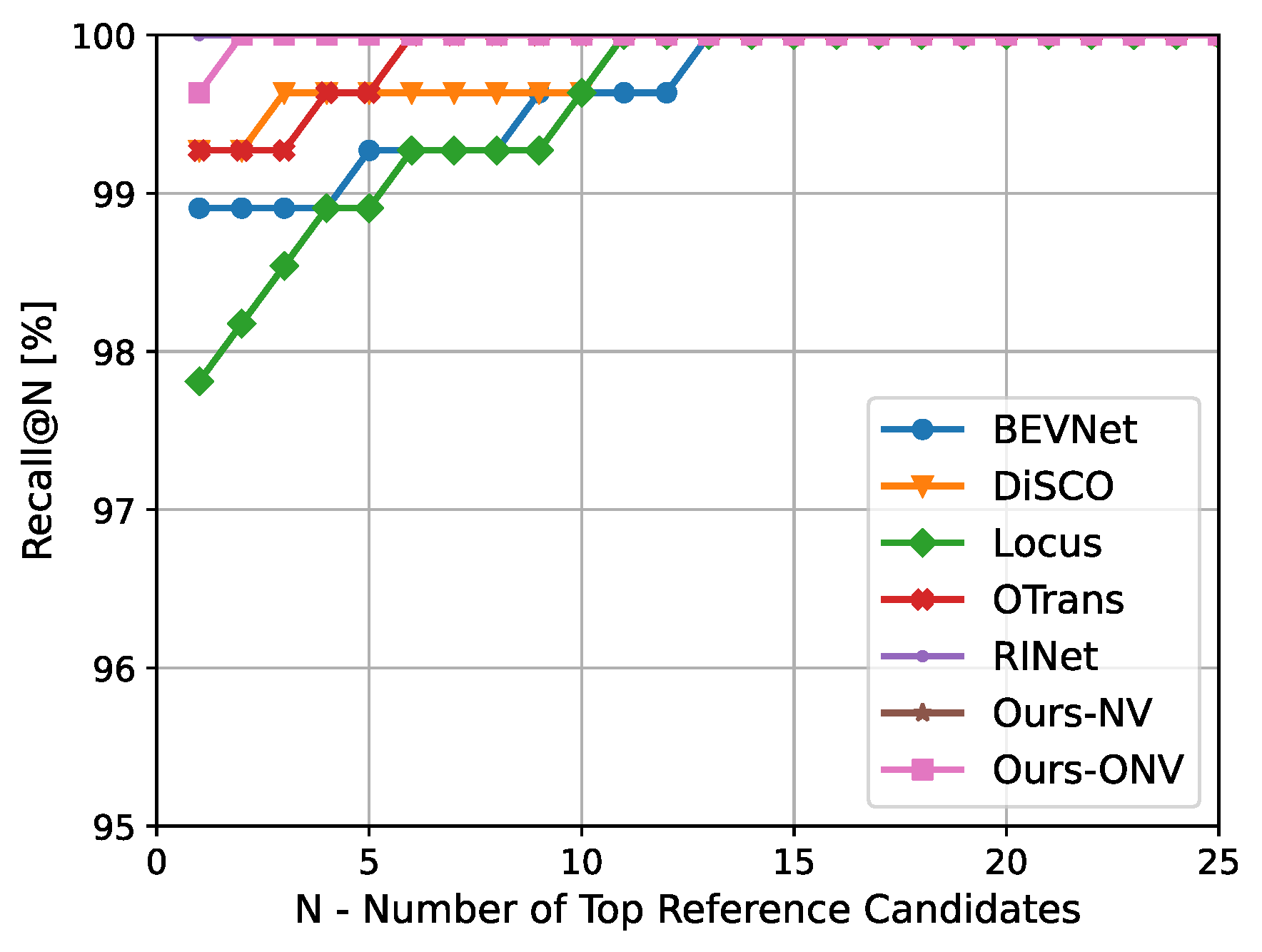
(d) 06

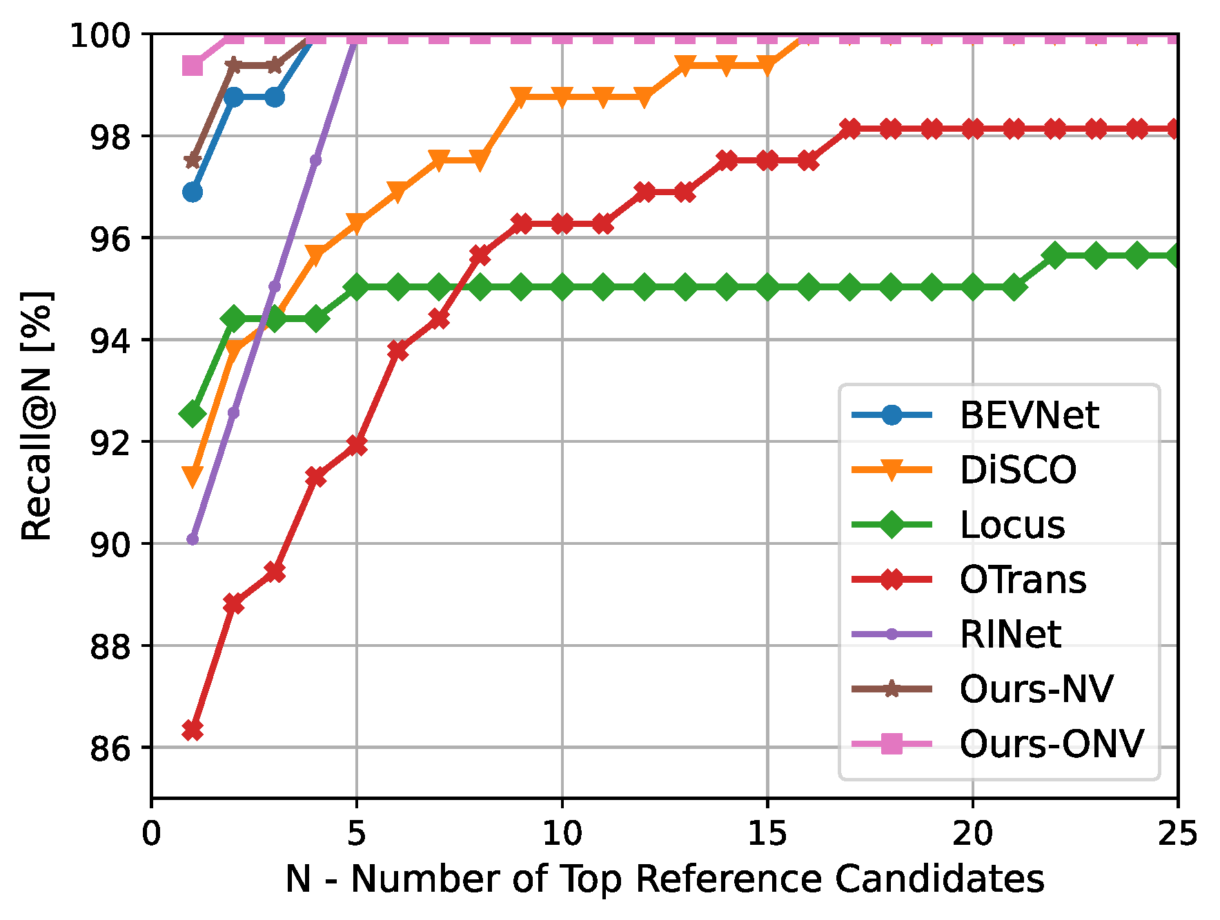
(e) 07

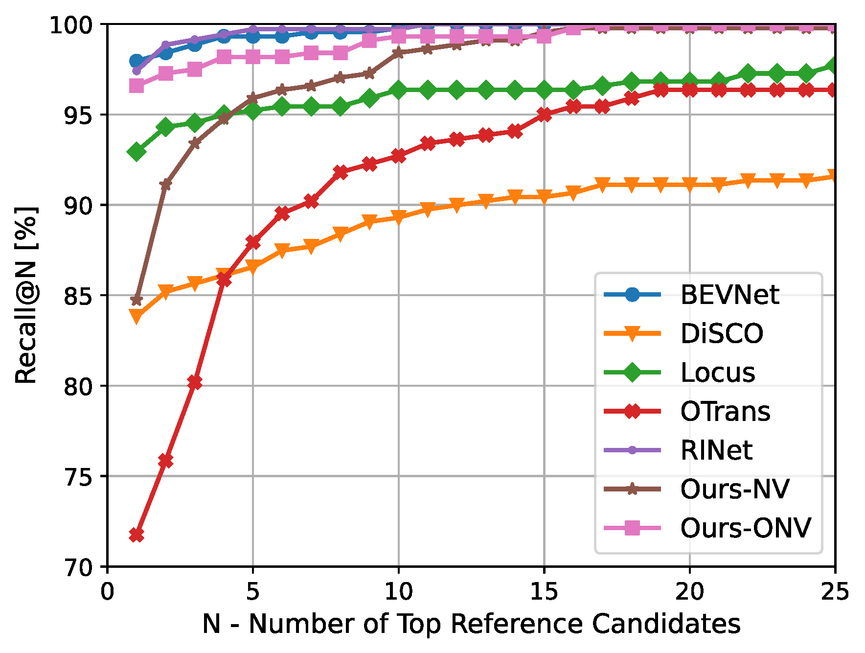
(f) 08

Figure 4: Recall@N for retrieval on KITTI dataset. OTrans denotes OverlapTransformer[8].

TABLE I: Recall@1 (%) and Recall@1% (%) on KITTI dataset

Methods	00	02	05	06	07	08	Mean
OTrans[8]	89.3/95.0	82.3/93.9	90.7/94.5	99.3/100.0	86.3/96.3	71.8/97.7	86.6/96.2
DiSCO[6]	90.3/97.7	83.7/91.9	88.1/96.2	99.3/100.0	91.3/98.8	83.8/93.2	89.4/96.3
Locus[19]	93.2/98.9	72.4/85.2	91.7/98.6	97.8/100.0	92.5/95.0	92.9/98.4	90.1/96.0
RINet[7]	98.9/100.0	80.0/99.7	97.6/99.6	100.0/100.0	90.1/100.0	97.4/100.0	94.0/99.9
BEVNet[10]	96.8/100.0	98.3/100.0	97.9/100.0	98.9/99.6	96.9/100.0	97.9/100.0	97.8/99.9
Ours-NV	95.9/100.0	91.0/99.7	94.3/99.5	99.6/100.0	97.5/100.0	84.7/100.0	93.8/99.9
Ours-ONV	96.8/100.0	97.4/99.7	97.6/99.5	99.6/100.0	99.4/100.0	96.6/100.0	97.9/99.9

• Recall@1 / Recall@1%. The best scores are marked in bold, and the second-best scores are underlined.

IV-A Datasets and Implementation Details

KITTI Odometry Benchmark. The KITTI odometry benchmark contains point clouds from various urban environments. The point clouds are collected using a Velodyne HDL-64E 3D laser scanner, which captures highly accurate 3D information. Moreover, the recording platform has a GPS/IMU location unit and RTK correction signals, providing ground truth poses[2]. The dataset includes 22 sequences, and we train our networks on the last 11 sequences with the ground truth trajectories provided by SemanticKITTI[35]. We evaluate the performance of our proposed method specifically on sequences 00, 02, 05, 06, 07, and 08, which contain revisited fragments, to detect loop closures.

Implementation Details. In the preprocessing stage, we transform the input point cloud into a BEV representation with a shape of $256\times 256\times 32$. The backbone network then extracts a sparse 2D feature map with a shape of $32\times 32\times 512$ using the SpConv[36] for improved speed. These feature maps are saved in a database for subsequent use by the global descriptor generator and overlap estimator.

For global descriptor generation, we use a NetVLAD layer with an intermediate feature dimension of 512, a maximum number of pooled samples of 1024, and 32 clusters. The output feature dimension is 1024, resulting in a final global descriptor vector length of 1024. The overlap estimator predicts the pairwise overlap region using a $1\times 32\times 32$ tensor and calculates the overlap score.

To train the descriptor generation network, we use point clouds less than 10m away from the query scan as positive examples and those more than 50m away as negative examples. We use a pre-trained model from [10] to extract BEV features and perform overlap estimation. During the evaluation, we exclude the previous 50 scans of the query scan, as they are too close. For candidate selection in the coarse search, we use $K=1\%$ (of the sequence length) as the number of candidates. We denote our method with only global descriptor matching as ours-NV and the complete coarse-to-fine method as ours-ONV.

IV-B Loop Closure Detection

In this section, we present the evaluation of the loop closure detection performance of our proposed framework and compare it with several state-of-the-art methods, including OverlapTransformer[8], DiSCO[6], Locus[19], RINet[7] and BEVNet[10]. We use recall@1 and recall@1% as the evaluation metric. The inference is considered correct if the distance between the matched scan and the query scan is less than 10m, otherwise incorrect. As shown in Tab. I, our method (ours-ONV) achieves the highest recall@1, with a score 0.1% higher than BEVNet and significantly higher than the other methods. Although the recall@1 of BEVNet and our method is similar, our approach has the advantage of being much less time-consuming. This is because our method significantly reduces the number of candidates when searching for matches, which leads to using fewer pairwise overlap estimates. Interestingly, the recall@1 of BEVNet on sequences 06 and 07 is lower than ours, which we believe is due to the increased probability of misestimation when increasing the number of candidates. Notably, our method can effectively and robustly detect reverse loop closures in sequence 08, which has only reverse loop closures. As a result, our method can achieve comparable loop closure performance to BEVNet, while requiring fewer computational resources.

In terms of recall@1%, RINet, BEVNet, Ours-NV, and Ours-ONV achieve a score close to 100%, while other methods achieve around 96%. The recall@1% of ours-NV indicates that our candidate selection process provides valid and accurate candidates, which is the foundation of our coarse-to-fine approach.

Furthermore, we evaluate the performance of the proposed method using recall@N on the KITTI dataset. As shown in Fig. 4, our method outperforms most baseline methods. And the average recall on KITTI dataset is shown in Fig. 5. The experimental results demonstrate the strong robustness and good generalization ability of our method for place recognition under challenging conditions.

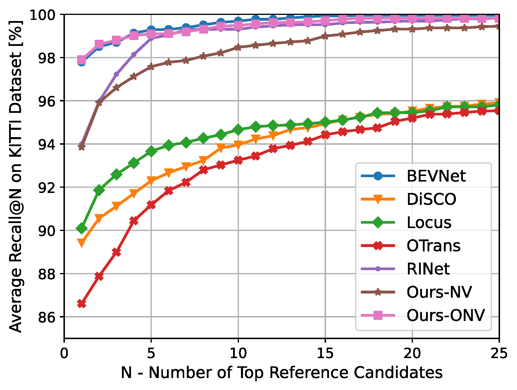
Figure 5: Average recall@N on KITTI dataset.

IV-C Ablation Study

In this section, we present our ablation studies on the proposed framework. We aim to evaluate the effectiveness of the coarse and fine stages of our approach independently. First, we investigate the impact of the global descriptor matching in the coarse stage. We choose the number of top references as $N=1,10,15,20,25,1\%$ to test recall@N for place recognition using only global descriptor matching, which we refer to as ours-NV. As shown in Tab. II, we observe that recall@1 alone is not sufficient to achieve outstanding performance, and the actual match places are not well recognized in sequence 08. However, as the number of candidates increases, the recall also increases significantly. When we use 1% of the total place as reference candidates, recall@1% achieves 99.9%. Therefore we choose $K=1\%$ as the candidate number for a coarse search.

Next, we evaluate the effect of candidate number K in the fine stage where the overlap estimation is applied. As shown in Tab. III, the recall@1 of only using global descriptor to detect loop closure (VLAD) is much lower than ours ONV-1%, which selects 1% of all scans as candidates by descriptor matching. Overall the recall@1 of our methods grows with the number of candidates, as we expected. Meanwhile, the recall of our framework is almost the same as BEVNet[10] (Overlap in Tab. III), while the latter is much more time-consuming. Comparing the results in Tab. II, we observe that the overlap estimation works well to detect loop closure using the proposed candidate selection approach.

In conclusion, the ablation studies validate that combining global descriptor matching and overlap estimation creates an effective and robust coarse-to-fine framework.

TABLE II: Recall@N (%) on KITTI dataset of ours-NV

	00	02	05	06	07	08	Mean
R@1	95.9	91.0	94.3	99.6	97.5	84.7	93.8
R@10	98.5	95.6	98.3	100.0	100.0	98.4	98.5
R@15	98.9	96.5	99.0	100.0	100.0	99.5	99.0
R@20	99.5	97.7	99.0	100.0	100.0	99.8	99.3
R@25	99.8	97.7	99.5	100.0	100.0	99.8	99.5
R@1%	100.0	99.7	99.5	100.0	100.0	100.0	99.9

• R@N denotes Recall@N.

TABLE III: Recall@1 (%) on KITTI dataset

Methods	00	02	05	06	07	08	Mean
VLAD	95.9	91.0	94.3	99.6	97.5	84.7	93.8
ONV-10	96.1	93.0	96.6	99.6	99.4	95.4	96.7
ONV-15	96.4	94.2	96.9	99.6	99.4	95.7	97.0
ONV-20	96.4	94.5	97.4	98.9	99.4	95.4	97.0
ONV-25	96.7	94.5	97.8	98.9	99.4	96.1	97.2
ONV-1%	96.8	97.4	97.6	99.6	99.4	96.6	97.9
Overlap	96.8	98.3	97.9	98.9	96.9	97.9	97.8

• VLAD means only using the global descriptor matching for retrieval, while Overlap means overlap estimation on all scans. ONV-K means overlap estimation on top-K candidates proposed by descriptor matching.

IV-D Runtime

In this section, we conduct experiments to evaluate the efficiency of our method and compare it with other methods. The experiments are performed on a system equipped with an Intel Core i7-7700 CPU with 3.60GHz and an Nvidia GeForce GTX 1080 Ti with 11GB memory, using sequence 00 which contains 4541 scans. Tab. IV shows that the candidate selection only takes 12.50ms, while the pairwise overlap estimation takes 7.13ms. We mainly compare the time consumption of ours-ONV with BEVNet. Since both methods use the same BEV feature maps, and they can be saved in the database without needing to be extracted each time, we mainly compare the time after feature extraction. For a query scan on sequence 00, ours-ONV costs $0.46\times 4541+12.50+7.13\times 4540\times 1\%=2425.06ms$, while BEVNet that performs overlap estimation for all references costs $7.13\times 4540=32370.20ms$. Notably, descriptors can also be saved in a database, eliminating the need to generate them for each search. Overall, Our method saves much time and has similar place recognition performance.

We also evaluate the runtime of other methods to compare the efficiency of descriptor generation. As shown in Tab. V, the global descriptor generation in our framework is very efficient compared to the other methods.

In summary, the matching of global descriptors provides a coarse but fast candidate selection, which is the foundation of the proposed coarse-to-fine framework. The runtime evaluation validates the effectiveness of our framework for selecting multiple candidates to improve loop closure detection speed.

TABLE IV: Runtime (ms) comparison of different modules

Module	Runtime
Voxelization	4.78
BEV Feature Extraction	2.34
Global Descriptor Generation	0.46
Candidate Selection	12.50
Pairwise Overlap Estimation	7.13

TABLE V: Runtime (ms) comparison of different methods

Methods	Preprocessing	Descriptor Generation	Total
OTrans	23.33	2.04	25.37
DiSCO	11.02	2.87	13.89
Locus	1166.49	613.96	1780.45
RINet	8.14	4.44	12.59
Ours-NV	4.78	2.80	7.58

• The preprocessing steps contain range image generation (OverlapTransformer), BEV representation construction (DiSCO and ours-NV), segments extraction (Locus), and descriptor generation (RINet). The batch size is set to 1 for all methods.

V CONCLUSION

In this paper, we propose a novel coarse-to-fine framework that provides a robust and efficient solution for LiDAR-based place recognition. The combination of global descriptor matching and overlap estimation allows for fast candidate selection and accurate loop closure detection. Moreover, our method achieves leading performance on the KITTI odometry benchmark compared to the state-of-the-art methods. While the framework has some limitations, such as the bulky and memory-intensive BEV features, future work will address these challenges and explore the integration of multi-modal data for improved place recognition.

References

- [1] S. Lowry, N. Sünderhauf, P. Newman, J. J. Leonard, D. Cox, P. Corke, and M. J. Milford, “Visual place recognition: A survey,” ieee transactions on robotics, vol. 32, no. 1, pp. 1–19, 2015.
- [2] A. Geiger, P. Lenz, C. Stiller, and R. Urtasun, “Vision meets robotics: The kitti dataset,” The International Journal of Robotics Research, vol. 32, no. 11, pp. 1231–1237, 2013.
- [3] M. A. Uy and G. H. Lee, “Pointnetvlad: Deep point cloud based retrieval for large-scale place recognition,” in Proceedings of the IEEE conference on computer vision and pattern recognition, pp. 4470–4479, 2018.
- [4] G. Kim and A. Kim, “Scan context: Egocentric spatial descriptor for place recognition within 3d point cloud map,” in 2018 IEEE/RSJ International Conference on Intelligent Robots and Systems (IROS), pp. 4802–4809, IEEE, 2018.
- [5] L. Li, X. Kong, X. Zhao, T. Huang, W. Li, F. Wen, H. Zhang, and Y. Liu, “Ssc: Semantic scan context for large-scale place recognition,” in 2021 IEEE/RSJ International Conference on Intelligent Robots and Systems (IROS), pp. 2092–2099, IEEE, 2021.
- [6] X. Xu, H. Yin, Z. Chen, Y. Li, Y. Wang, and R. Xiong, “Disco: Differentiable scan context with orientation,” IEEE Robotics and Automation Letters, vol. 6, no. 2, pp. 2791–2798, 2021.
- [7] L. Li, X. Kong, X. Zhao, T. Huang, W. Li, F. Wen, H. Zhang, and Y. Liu, “Rinet: Efficient 3d lidar-based place recognition using rotation invariant neural network,” IEEE Robotics and Automation Letters, vol. 7, no. 2, pp. 4321–4328, 2022.
- [8] J. Ma, J. Zhang, J. Xu, R. Ai, W. Gu, and X. Chen, “Overlaptransformer: An efficient and yaw-angle-invariant transformer network for lidar-based place recognition,” IEEE Robotics and Automation Letters, vol. 7, no. 3, pp. 6958–6965, 2022.
- [9] S. Huang, Z. Gojcic, M. Usvyatsov, A. Wieser, and K. Schindler, “Predator: Registration of 3d point clouds with low overlap,” in Proceedings of the IEEE/CVF Conference on computer vision and pattern recognition, pp. 4267–4276, 2021.
- [10] L. Li, W. Ding, Y. Wen, Y. Liang, Y. Liu, and G. Wan, “A unified bev model for joint learning of 3d local features and overlap estimation,” arXiv preprint arXiv:2302.14511, 2023.
- [11] R. Arandjelovic, P. Gronat, A. Torii, T. Pajdla, and J. Sivic, “Netvlad: Cnn architecture for weakly supervised place recognition,” in Proceedings of the IEEE conference on computer vision and pattern recognition, pp. 5297–5307, 2016.
- [12] H. Li, C. Sima, J. Dai, W. Wang, L. Lu, H. Wang, E. Xie, Z. Li, H. Deng, H. Tian, et al., “Delving into the devils of bird’s-eye-view perception: A review, evaluation and recipe,” arXiv preprint arXiv:2209.05324, 2022.
- [13] J. Guo, P. V. K. Borges, C. Park, and A. Gawel, “Local descriptor for robust place recognition using lidar intensity,” IEEE Robotics and Automation Letters, vol. 4, no. 2, pp. 1470–1477, 2019.
- [14] Y. Xia, Y. Xu, S. Li, R. Wang, J. Du, D. Cremers, and U. Stilla, “Soe-net: A self-attention and orientation encoding network for point cloud based place recognition,” in Proceedings of the IEEE/CVF Conference on Computer Vision and Pattern Recognition (CVPR), pp. 11348–11357, June 2021.
- [15] L. Luo, S.-Y. Cao, B. Han, H.-L. Shen, and J. Li, “Bvmatch: Lidar-based place recognition using bird’s-eye view images,” IEEE Robotics and Automation Letters, vol. 6, no. 3, pp. 6076–6083, 2021.
- [16] L. He, X. Wang, and H. Zhang, “M2dp: A novel 3d point cloud descriptor and its application in loop closure detection,” in 2016 IEEE/RSJ International Conference on Intelligent Robots and Systems (IROS), pp. 231–237, 2016.
- [17] C. R. Qi, H. Su, K. Mo, and L. J. Guibas, “Pointnet: Deep learning on point sets for 3d classification and segmentation,” in Proceedings of the IEEE conference on computer vision and pattern recognition, pp. 652–660, 2017.
- [18] M. Y. Chang, S. Yeon, S. Ryu, and D. Lee, “Spoxelnet: spherical voxel-based deep place recognition for 3d point clouds of crowded indoor spaces,” in 2020 IEEE/RSJ International Conference on Intelligent Robots and Systems (IROS), pp. 8564–8570, IEEE, 2020.
- [19] K. Vidanapathirana, P. Moghadam, B. Harwood, M. Zhao, S. Sridharan, and C. Fookes, “Locus: Lidar-based place recognition using spatiotemporal higher-order pooling,” in 2021 IEEE International Conference on Robotics and Automation (ICRA), pp. 5075–5081, IEEE, 2021.
- [20] X. Kong, X. Yang, G. Zhai, X. Zhao, X. Zeng, M. Wang, Y. Liu, W. Li, and F. Wen, “Semantic graph based place recognition for 3d point clouds,” in 2020 IEEE/RSJ International Conference on Intelligent Robots and Systems (IROS), pp. 8216–8223, IEEE, 2020.
- [21] J. Komorowski, “Minkloc3d: Point cloud based large-scale place recognition,” in Proceedings of the IEEE/CVF Winter Conference on Applications of Computer Vision, pp. 1790–1799, 2021.
- [22] T.-Y. Lin, P. Dollár, R. Girshick, K. He, B. Hariharan, and S. Belongie, “Feature pyramid networks for object detection,” in Proceedings of the IEEE conference on computer vision and pattern recognition, pp. 2117–2125, 2017.
- [23] F. Radenović, G. Tolias, and O. Chum, “Fine-tuning cnn image retrieval with no human annotation,” IEEE transactions on pattern analysis and machine intelligence, vol. 41, no. 7, pp. 1655–1668, 2018.
- [24] P. Yin, L. Xu, J. Zhang, and H. Choset, “Fusionvlad: A multi-view deep fusion networks for viewpoint-free 3d place recognition,” Ieee Robotics and Automation Letters, vol. 6, no. 2, pp. 2304–2310, 2021.
- [25] K. Vidanapathirana, M. Ramezani, P. Moghadam, S. Sridharan, and C. Fookes, “Logg3d-net: Locally guided global descriptor learning for 3d place recognition,” in 2022 International Conference on Robotics and Automation (ICRA), pp. 2215–2221, 2022.
- [26] Y. Hou, H. Zhang, and S. Zhou, “Bocnf: efficient image matching with bag of convnet features for scalable and robust visual place recognition,” Autonomous Robots, vol. 42, pp. 1169–1185, 2018.
- [27] P.-E. Sarlin, C. Cadena, R. Siegwart, and M. Dymczyk, “From coarse to fine: Robust hierarchical localization at large scale,” in Proceedings of the IEEE/CVF Conference on Computer Vision and Pattern Recognition, pp. 12716–12725, 2019.
- [28] J. Qi, R. Wang, C. Wang, and X. Cao, “Coarse-to-fine visual place recognition,” in Neural Information Processing: 28th International Conference, pp. 28–39, Springer, 2021.
- [29] S. Garg, N. Suenderhauf, and M. Milford, “Semantic–geometric visual place recognition: a new perspective for reconciling opposing views,” The International Journal of Robotics Research, vol. 41, no. 6, pp. 573–598, 2022.
- [30] K. P. Cop, P. V. Borges, and R. Dubé, “Delight: An efficient descriptor for global localisation using lidar intensities,” in 2018 IEEE International Conference on Robotics and Automation (ICRA), pp. 3653–3660, IEEE, 2018.
- [31] Y. Gong, F. Sun, J. Yuan, W. Zhu, and Q. Sun, “A two-level framework for place recognition with 3d lidar based on spatial relation graph,” Pattern Recognition, vol. 120, p. 108171, 2021.
- [32] Z. Qin, H. Yu, C. Wang, Y. Guo, Y. Peng, and K. Xu, “Geometric transformer for fast and robust point cloud registration,” in Proceedings of the IEEE/CVF Conference on Computer Vision and Pattern Recognition, pp. 11143–11152, 2022.
- [33] H. Chen, Z. Wei, Y. Xu, M. Wei, and J. Wang, “Imlovenet: Misaligned image-supported registration network for low-overlap point cloud pairs,” in ACM SIGGRAPH 2022 Conference Proceedings, pp. 1–9, 2022.
- [34] Y. Sun, C. Cheng, Y. Zhang, C. Zhang, L. Zheng, Z. Wang, and Y. Wei, “Circle loss: A unified perspective of pair similarity optimization,” in Proceedings of the IEEE/CVF conference on computer vision and pattern recognition, pp. 6398–6407, 2020.
- [35] J. Behley, M. Garbade, A. Milioto, J. Quenzel, S. Behnke, C. Stachniss, and J. Gall, “Semantickitti: A dataset for semantic scene understanding of lidar sequences,” in Proceedings of the IEEE/CVF international conference on computer vision, pp. 9297–9307, 2019.
- [36] Y. Yan, Y. Mao, and B. Li, “Second: Sparsely embedded convolutional detection,” Sensors, vol. 18, no. 10, p. 3337, 2018.