Continuous-Time Zeroth-Order Dynamics with Projection Maps: Model-Free Feedback Optimization with Safety Guarantees

Abstract

This paper introduces a class of model-free feedback methods for solving generic constrained optimization problems where the specific mathematical forms of the objective and constraint functions are not available. The proposed methods, termed Projected Zeroth-Order (P-ZO) dynamics, incorporate projection maps into a class of continuous-time model-free dynamics that make use of periodic dithering for the purpose of gradient learning. In particular, the proposed P-ZO algorithms can be interpreted as new extremum-seeking algorithms that autonomously drive an unknown system toward a neighborhood of the set of solutions of an optimization problem using only output feedback, while systematically guaranteeing that the input trajectories remain in a feasible set for all times. In this way, the P-ZO algorithms can properly handle hard and asymptotical constraints in model-free optimization problems without using penalty terms or barrier functions. Moreover, the proposed dynamics have suitable robustness properties with respect to small bounded additive disturbances on the states and dynamics, a property that is fundamental for practical real-world implementations. Additional tracking results for time-varying and switching cost functions are also derived under stronger convexity and smoothness assumptions and using tools from hybrid dynamical systems. Numerical examples are presented throughout the paper to illustrate the above results.

I INTRODUCTION

This paper studies the design of model-free feedback control algorithms for autonomously steering a plant toward the set of solutions of an optimization problem using high-frequency dither signals. This type of feedback control design has recently attracted considerable attention, due to successful applications in power grids, communication networks, and mobile robots; see [1] and references therein.

The designing of these controllers for practical applications is particularly challenging because of two major obstacles: one is the lack of accurate models of the system, as many real-world systems are too complex to derive tractable mathematical equations that accurately describe their behavior in unknown or dynamic environments; the other obstacle is to meet safety requirements by properly handling various constraints, including physical laws, control saturation, capacity and budget limits, etc. This paper introduces a class of algorithms that can overcome both of these obstacles and are suitable for the solution of model-free constrained optimization problems describing safety-critical applications.

I-A Literature Review

To address the problem of unknown system models, real-time model-free control and optimization schemes have been extensively studied. In these approaches, instead of pre-establishing a complex and often static/stationary system model from first principles and historical data, adaptive control algorithms probe the unknown plant and learn its optimal operation points using real-time output feedback. Such techniques, called extremum seeking (ES) controllers, leverage multi-time scale principles in control theory to steer dynamical systems towards an optimal steady state operation, while preserving closed-loop stability guarantees. ES techniques date back to the early 1920s [2]. However, the first general stability analysis for nonlinear systems was presented in the 2000s in [3] using averaging-based methods, and in [4] using sampled-data approaches based on finite-differences approximations. Since these methods make use of only measurements of the objective function, ES exhibits a close connection with discrete-time zeroth-order optimization dynamics [5, 6]. In the continuous-time and finite-dimensional setting, ES algorithms have been further advanced during the last two decades using more general analytical and design techniques for continuous-time systems, see [7, 8, 9, 10, 11].

However, despite the theoretical advances and practical applications in ES, one of the major challenges of existing schemes is how to guarantee the systematic satisfaction of hard and asymptotical constraints simultaneously. Hard constraints refer to physical or safety-critical constraints that need to be satisfied by the actions of the controller at all times, e.g. saturation or actuator capacity limits, the generation capacity of a power plant, etc. On the other hand, asymptotic constraints refer to soft physical limits or performance requirements that can be violated temporarily during transient processes but should be met in the long-term steady state, e.g., the thermal limits of power lines and voltage limits imposed by industrial standards, the comfortable temperature ranges required in building climate control, etc. Properly handling these two types of constraints is essential to ensure stability and optimality in real-time optimization algorithms.

In the context of ES, most of the approaches and stability results have been developed for unconstrained optimization problems. For optimization problems with hard constraints, the majority of the results and schemes have been limited to methods that integrate barrier or penalty functions in the cost [12, 13, 14, 15, 16, 17], which can limit the type and number of constraints that can be handled by the algorithms. In [18, 19, 20, 21, 22], ES algorithms were introduced to solve optimization problems with constraints defined by certain Euclidean smooth manifolds and Lie Groups. These schemes, however, do not incorporate soft constraints in the optimization problem, and can only handle boundaryless manifolds. Anti-windup techniques in ES for problems that involve saturation were studied in [23], and ES with output constraints were studied in [24] using boundary tracing techniques. Switching ES algorithms that emulate sliding-mode techniques were also presented in [25] to handle hard constraints in time-varying problems. More recently, an innovative approach that combines safety filters and ES was introduced in [26] using control barrier functions and quadratic programming. To handle soft constraints, ES approaches based on saddle flows have also been studied in [27, 28, 29, 30]. Finally, more closely related to our setting are the works [31, 32], which considered ES algorithms with certain projection maps for scalar problems [31], and numerical studies of Nash-seeking problems with box constraints [32, Section V-B].

I-B Contributions and Organization

This paper introduces a class of continuous-time projected zeroth-order (P-ZO) algorithms for solving generic constrained optimization problems with both hard and asymptotical constraints. Based on ES and two different types of projection maps, the proposed P-ZO methods can be interpreted as model-free feedback controllers that steer a plant towards the set of solutions of an optimization problem with hard and soft constraints, using only measurements of the objective and constraint functions. In particular, we explain the main advantages and innovations of the proposed algorithms below:

(a) Model-Free Methods: We study a class of optimization algorithms that use only measurements or evaluations of the objective function and the constraints, i.e., zeroth-order information. In this way, the algorithms do not require knowledge of the mathematical forms of the expressions that define the optimization problem, or their gradients. We show that, under suitable tuning of the control parameters, the trajectories of the proposed model-free ZO algorithms can approximate the behavior of continuous and discontinuous first-order model-based dynamics [33, 34, 1]. By exploiting real-time output feedback, the proposed algorithms are inherently robust and adaptive to time-varying unknown disturbances, and for a general class of objective functions, potentially time-varying or switching between a finite collection of candidates.

(b) Safety and Optimality via Hard and Soft Constraints: The proposed algorithms can satisfy safety-critical constraints at all times by using continuous or discontinuous projection maps. The systematic incorporation of these mappings into ES vector fields remained mostly unexplored in the literature, and our results show that they can be safely used in feedback loops to solve optimization problems with hard constraints. In the context of ES, to allow for enough exploration via dithering, the projection maps are applied to a shrunken feasible set that can be made arbitrarily close to the nominal feasible set by decreasing the amplitude of the dithers. In this way, the algorithms are able to provide suitable evolution directions near the boundary of the feasible set, achieving a property of “practical safety”, similar in spirit to the one studied in [26]. In addition to the hard constraints, the proposed controllers are also able to simultaneously handle soft constraints via primal-dual ES vector fields, thus achieving safety and optimality in a variety of model-free optimization problems.

(c) Stability and Performance Guarantees: We leverage averaging and singular perturbation theory for non-smooth (and hybrid) systems, as well as Lyapunov-based arguments, to show that the proposed dynamics can guarantee convergence to an arbitrarily small neighborhood of the optimal set, from arbitrarily large compact sets of initial conditions in the feasible set. Moreover, by exploiting the well-posedness of the dynamics and the optimization problem, the algorithms also guarantee suitable robustness properties with respect to arbitrarily small bounded additive disturbances acting on the states and dynamics of the closed-loop system. This is a fundamental property for practical applications and is non-trivial to achieve in model-free algorithms. We also provide tracking bounds for time-varying optimization problems using (practical) input-to-state stability tools, and we provide stability results for a class of ES problems with unknown switching objective functions, which have remained mostly unexplored in the literature.

Earlier, partial results of this paper appeared in the conference paper [35]. The results of [35] are dedicated only to a particular optimal voltage control problem in power systems using only one of the algorithms studied in this paper. In contrast to [35], in this paper, we consider a generic constrained optimization problem and we study two different types of projection maps (continuous and discontinuous), which require different analytical tools and lead to two different algorithms. Additionally, we present novel tracking results for time-varying optimization problems and problems with switching costs, and we establish robustness guarantees for all the algorithms. Unlike [35], we also present the complete proofs of the results, as well as novel illustrative examples.

The remainder of this paper is organized as follows: Section II introduces the notation and the preliminaries. Section III presents the problem formulation. Section IV introduces the projected ZO dynamics that incorporate Lipschitz projection maps, and establishes results for static maps, time-varying maps, and switching maps. Section V considers projected gradient-based ZO dynamics with discontinuous projections. Section VI presents the analysis and proofs. Numerical experiments are presented throughout the paper to illustrate the main ideas and results. The paper ends with conclusions presented in Section VII.

II NOTATION AND PRELIMINARIES

II-A Notation

We use unbolded lower-case letters for scalars and bolded lower-case letters for column vectors. We use $\mathbb{R}_{+}:=[0,+\infty)$ to denote the set of non-negative real values and use $\mathbb{B}$ to denote a closed unit ball of appropriate dimension. We use $||\cdot||$ to denote the Euclidean norm of a vector and use $[\mathbf{x};\mathbf{y}]:=[\mathbf{x}^{\top},\mathbf{y}^{\top}]^{\top}$ to denote the column merge of column vectors $\mathbf{x},\mathbf{y}$. Given a positive integer $n$, we define the index set $[n]:=\{1,\cdots,n\}$. The distance between a point $\mathbf{x}\in\mathbb{R}^{n}$ and a nonempty closed convex set $\mathcal{X}\subseteq\mathbb{R}^{n}$ is denoted as $||\mathbf{x}||_{\mathcal{X}}:=\underset{\mathbf{\mathbf{y}}\in\mathcal{X}}{\inf}\,||\mathbf{y}-\mathbf{x}||$; and the Euclidean projection of $\mathbf{x}$ onto the set $\mathcal{X}$ is defined as

$$\mathcal{P}_{\mathcal{X}}(\mathbf{x}):=\underset{\mathbf{y}\in\mathcal{X}}{\mathrm{arg\,inf}}\,||\mathbf{y}-\mathbf{x}||.$$ (1)

The norm cone to a set $\mathcal{X}$ at a point $\mathbf{x}\in\mathcal{X}$ is defined as

$$N_{\mathcal{X}}(\mathbf{x}):=\left\{\mathbf{s}\in\mathbb{R}^{n}:\,\mathbf{s}^{\top}(\mathbf{y}-\mathbf{x})\leq 0,\ \forall~{}\mathbf{y}\in\mathcal{X}\right\}.$$ (2)

The tangent cone to $\mathcal{X}$ at a point $\mathbf{x}\in\mathcal{X}$ is defined as

$$T_{\mathcal{X}}(\mathbf{x}):=\left\{\mathbf{d}\in\mathbb{R}^{n}:\,\mathbf{d}^{\top}\mathbf{s}\leq 0,\,\forall~{}\mathbf{s}\in N_{\mathcal{X}}(\mathbf{x})\right\},$$ (3)

which is the polar cone of the normal cone $N_{\mathcal{X}}(\mathbf{x})$. A continuous function $\beta(r,s):\mathbb{R}_{+}\times\mathbb{R}_{+}\to\mathbb{R}_{+}$ is said to be of class-$\mathcal{KL}$ if it is zero at zero, non-decreasing in its first argument $r$, non-increasing in the second argument $s$, $\lim_{r\to 0^{+}}\beta(r,s)=0$ for each $s$, and $\lim_{s\to\infty}\beta(r,s)=0$ for each $r$ [36, Def. 3.38].

In this paper, we will consider constrained dynamical systems in the form:

$$\mathbf{x}\in C,~{}~{}~{}\dot{\mathbf{x}}\in F(\mathbf{x}),$$ (4)

where $\mathbf{x}\in\mathbb{R}^{n}$ is the state, $C$ is the flow set, and $F:\mathbb{R}^{n}\rightrightarrows\mathbb{R}^{n}$ is the flow map, which can be set-valued. We use $\dot{\mathbf{x}}=\frac{d\mathbf{x}(t)}{dt}$ to denote the time derivative of the function $t\mapsto\mathbf{x}(t)$. A function $\mathbf{x}$ is said to be a (Caratheodory) solution to (4) if 1) $t\mapsto\mathbf{x}(t)$ is absolutely continuous on each compact sub-interval of its domain $\text{dom}(\mathbf{x})$; 2) $\mathbf{x}(0)\in{C}$; and 3) $\dot{\mathbf{x}}(t)\in F(\mathbf{x}(t))$ and $\mathbf{x}(t)\in C$ for almost all $t\in\text{dom}(\mathbf{x})$ [37, pp. 4]. The solution $\mathbf{x}$ is said to be complete if $\text{dom}(\mathbf{x})=[0,\infty)$. If the flow map $F$ is single-valued, (4) reduces to an ordinary differential equation. If $F$ is also continuous, solutions $\mathbf{x}$ to (4) are continuously differentiable functions. In addition, if $F$ is locally Lipschitz, then solutions of (4) are unique.

II-B Preliminaries on Extremum Seeking Control

Extremum Seeking (ES) control is a type of adaptive control that is able to steer a plant towards a state that optimizes a particular steady-state performance metric using real-time output feedback. These types of controllers can be seen as continuous-time ZO optimization algorithms with (uniform) convergence and stability guarantees. To explain the rationale behind these algorithms, we consider the optimization problem

$$\min_{x}f(x),$$ (5)

where $f:\mathbb{R}\to\mathbb{R}$ is a continuously differentiable function. A standard approach to finding the minimizer of $f$ is to use a gradient descent flow in the form $\dot{{x}}=-k_{x}\cdot\frac{df(x)}{dx}$, where the gain $k_{x}$ defines the rate of evolution of the system. However, when the derivative of $f$ is unknown, gradient flows cannot be directly implemented, and instead, model-free techniques are required. To address this issue, ES approximates the behavior of the gradient flow by adding a high-frequency periodic probing signal $\varepsilon_{a}\hat{\mu}(t)$ with amplitude $\varepsilon_{a}$ to the nominal input of the plant. The resulting output $y=f(x+\varepsilon_{a}\hat{\mu}(t))$, which is assumed to be available for measurements, is then multiplied by the same probing signal $\hat{\mu}(t)$, and further normalized by the constant $2/\varepsilon_{a}$. The loop is closed with an integrator with a negative gain $-k_{x}$, leading to the ES dynamics:

$$\dot{x}=-k_{x}\frac{2}{\varepsilon_{a}}f\left(x+\varepsilon_{a}\hat{\mu}(t)\right)\hat{\mu}(t).$$ (6)

When the frequency of $\hat{\mu}(\cdot)$ is sufficiently large compared to the rate of evolution $k_{x}$, the ES dynamics (6) exhibits a time scale separation property that allows to approximate the behavior of $x$ based on the average of the vector field of (6). For example, consider the use of a sinusoidal signal as the probing single, i.e., $\hat{\mu}(t):=\sin(\omega t)$. With large $\omega>0$ and small $\varepsilon_{a}$, we consider the Taylor expansion of $f$:

$$f(x+\varepsilon_{a}\sin(\omega t))=f(x)+\varepsilon_{a}\sin(\omega t)\frac{df(x)}{dx}+\mathcal{O}(\varepsilon_{a}^{2}).$$

By computing the average of the vector field of (6) over one period $T=\frac{2\pi}{\omega}$ of the probing signal, one obtains

$$\dot{{x}} =\frac{1}{T}\int_{0}^{T}\!\!-k_{x}\frac{2}{\varepsilon_{a}}f(x+\varepsilon_{a}\sin(\omega t))\sin(\omega t)\,dt$$

$$=-\frac{k_{x}}{T}\int_{0}^{T}\!\!2\sin^{2}(\omega t)\frac{df(x)}{dx}+\mathcal{O}(\varepsilon_{a})\,dt,$$

$$=-k_{x}\frac{df(x)}{dx}+\mathcal{O}(\varepsilon_{a}):=h_{\text{ave}}(x)$$ (7)

where $\mathcal{O}(\varepsilon_{a})$ denotes high-order terms, bounded on compact sets, that vanish as $\varepsilon_{a}\to 0^{+}$. The average system (II-B) is essentially an $\mathcal{O}(\varepsilon_{a})$-perturbed gradient descent flow. Under suitable assumptions on $f$, averaging theory and perturbation theory show that the trajectories of (6) will approximate those of (II-B) (on compact sets and compact time intervals) as $\varepsilon_{a}\to 0^{+}$ and as $\omega\to 0^{+}$ [38, Theorem 1]. Uniform stability properties of gradient flows can then be leveraged to establish stability results for (6) in the infinite horizon [38, Theorem 2]. This analysis can also be applied to the multi-variable case using an appropriate choice of the (vector) frequencies $\omega$, and to other architectures using Lie-bracket averaging theory that results in a similar average system [9, 10].

III PROBLEM FORMULATION

In contrast to (5), in this paper, we consider generic constrained optimization problems in the form:

Obj. $$\min_{\mathbf{x}}\,f(\mathbf{x})$$ (8a)

s.t. $$\ \mathbf{x}\in\mathcal{X}$$ (8b)

$$\ g_{j}(\mathbf{x})\leq 0,\qquad j\in[m],$$ (8c)

where $\mathbf{x}\in\mathbb{R}^{n}$ is the decision variable, $f:\mathbb{R}^{n}\to\mathbb{R}$ is the objective function, $\mathcal{X}\subseteq\mathbb{R}^{n}$ denotes the feasible set of $\mathbf{x}$, and the vector-valued function $\mathbf{g}:=[g_{1};g_{2};\cdots;g_{m}]:\mathbb{R}^{n}\to\mathbb{R}^{m}$ describes additional inequality constraints on $\mathbf{x}$. The set of the optimal solutions of (8) is denoted as $\mathcal{X}^{*}\subset\mathbb{R}^{n}$.

Information Availability: We consider the problem setting where the feasible set $\mathcal{X}$ is known but the mathematical forms of $f(\cdot)$ and $\mathbf{g}(\cdot)$ are unknown. In this case, one can only query (in real-time) the values of $f(\mathbf{x})$ and $\mathbf{g}(\mathbf{x})$ for a given $\mathbf{x}$. That is, the optimization solver can only access the zeroth-order information of $f(\cdot)$ and $\mathbf{g}(\cdot)$, but not their (first-order) gradients or (second-order) Hessian information.

The motivation and rationale of the above problem setting are explained below:

• The above problem is motivated by the feedback control design that seeks to steer an unknown plant in real time to an optimal solution of problem (8). Here, we model the plant using the static input-to-output maps $f(\cdot)$ and $\mathbf{g}(\cdot)$ to approximate its dynamics. The validity of this approximation lies in the fact that in many applications the plant is a stable dynamical system that converges to a steady state in a much faster time scale compared to the controller. The steady-state approximation of the plant can then be justified using singular perturbation results for nonlinear systems [38, Theorem 2], provided that the time-scale separation is sufficiently large.

• For many complex engineering systems, their models, captured by the maps $f(\cdot)$ and $\mathbf{g}(\cdot)$, may be unknown, unavailable, or too costly to estimate. On the other hand, the widespread deployment of smart meters and sensors provides real-time measurements of the system outputs. These measurements can be interpreted as the function evaluations of $f(\cdot)$ and $\mathbf{g}(\cdot)$ and can be used as the system feedback to circumvent the unknown model information.

• In problem (8), we distinguish hard constraints, modeled by $\mathcal{X}$, and asymptotic constraints, modeled by the inequalities (8c). Thus, the constraints imposed by $\mathcal{X}$ (8b) must be satisfied at all times, while inequalities (8c) may be violated during the transient process but should be satisfied in the steady states.

This paper aims to develop model-free feedback optimization algorithms that are able to solve problem (8) using only zeroth-order information, while simultaneously satisfying hard and asymptotic constraints. To achieve these goals, in Sections IV and V, we will study a class of ZO feedback optimization algorithms that are based on ES and incorporate two types of projection maps. To guarantee that problem (8) is well-posed, throughout this paper we will make the following assumptions, which, as discussed later, can be used to relax standard global convexity assumptions considered in the literature of ES.

Assumption 1.

The feasible set $\mathcal{X}$ is nonempty, closed, and convex. The functions $f$ and $g_{1},\cdots,g_{m}$ are convex and continuously differentiable on an open set containing $\mathcal{X}$. The function $f$ is radially unbounded. $\square$

Assumption 2.

Problem (8) has a finite optimum and the Slater’s conditions hold. Moreover, the set of optimal solutions $\mathcal{X}^{*}$ is compact. $\square$

IV MODEL-FREE FEEDBACK OPTIMIZATION WITH LIPSCHITZ PROJECTIONS

In this section, we introduce a class of gradient-based continuous-time ZO algorithms that incorporate Lipschitz continuous projection maps. We term these algorithms as the projected gradient-based zeroth-order (P-GZO) dynamics. We first study a reduced version of (8) that considers only the hard constraint (8b), i.e., we consider the problem:

$$\min_{\mathbf{x}\in\mathcal{X}}\ f(\mathbf{x}).$$ (9)

For this problem, we establish stability, safety, and tracking results under the P-GZO dynamics. After this, we develop results for the case when $f$ is dynamically drawn from a finite collection of cost functions that share the same minimizer, a problem that emerges in systems with switching plants. Lastly, we further incorporate the constraints (8c) using a projected primal-dual zeroth-order (P-PDZO) algorithm.

IV-A GZO Dynamics with Lipschitz Projection

To solve (9), we develop the following dynamics termed projected gradient zeroth-order (P-GZO) dynamics:

$$\dot{\mathbf{x}} =k_{x}\Big{(}\mathcal{P}_{\mathcal{X}}(\mathbf{x}-\alpha_{x}\,\bm{\xi})-\mathbf{x}\Big{)},$$ (10a)

$$\dot{{\bm{\xi}}} =\frac{1}{\varepsilon_{\xi}}\Big{(}-{\bm{\xi}}+\frac{2}{\varepsilon_{a}}f(\hat{\mathbf{x}})\hat{\bm{\mu}}\Big{)},$$ (10b)

$$\dot{{\bm{\mu}}} =\frac{1}{\varepsilon_{\omega}}\Lambda_{\kappa}{\bm{\mu}},$$ (10c)

where $k_{x},\alpha_{x},\varepsilon_{\xi},\varepsilon_{a},\varepsilon_{\omega}\!>\!0$ are tunable parameters. The dynamics (10a) incorporates a Lipschitz projection map of the form (1) to ensure that $\mathbf{x}$ stays within the feasible set $\mathcal{X}$. The dynamics (10b) estimates the gradient $\nabla f$ with a new state $\bm{\xi}\in\mathbb{R}^{n}$, whose dynamics depend on the measured output $y=f(\hat{\mathbf{x}})$, where $\hat{\mathbf{x}}$ is the perturbed input defined as

$$\hat{\mathbf{x}}:=\mathbf{x}+\varepsilon_{a}\hat{\bm{\mu}}.$$ (11)

In (11), $\hat{\bm{\mu}}:\mathbb{R}_{\geq 0}\to\mathbb{R}^{n}$ is a vector-valued periodic dither signal that is generated by the linear dynamic oscillator (10c). Specifically, the vector $\hat{\bm{\mu}}$ collects all the odd entries of the state ${\bm{\mu}}\in\mathbb{R}^{2n}$, i.e.,

$$\hat{\bm{\mu}} :=[{\mu}_{1},{\mu}_{3},{\mu}_{5},\cdots,{\mu}_{2n-1}]^{\top}.$$ (12)

The matrix $\Lambda_{\kappa}\in\mathbb{R}^{2n\times 2n}$ in (10c) is block diagonal, with the $i$-th diagonal block given by

$$\Lambda_{\kappa_{i}}=\left[\begin{array}[]{cc}0&-2\pi\kappa_{i}\\ 2\pi\kappa_{i}&0\end{array}\right]\in\mathbb{R}^{2\times 2},\quad i\in[n],$$ (13)

which is parameterized by the tunable constant $\kappa_{i}>0$. Hence, (10c) describes $n$ autonomous oscillators, whose solutions ${\bm{\mu}}$ can be explicitly computed as

$$\begin{split}{\mu}_{i}(t)={\mu}_{i}(0)\sin\left(\frac{2\pi\kappa_{i}}{\varepsilon_{\omega}}t\right)&+\mu_{i+1}(0)\cos\big{(}\frac{2\pi\kappa_{i}}{\varepsilon_{\omega}}t\big{)},\\ &\qquad\forall\,i=1,3,\cdots,2n\!-\!1,\end{split}$$ (14)

and we choose initial conditions that satisfy

$${\mu}_{i}(0)^{2}+{\mu}_{i+1}(0)^{2}=1.$$ (15)

For example, when ${\mu}_{i}(0)=1$ and ${\mu}_{i+1}(0)=0$ for $i=1,3,\cdots,2n\!-\!1$, equation (12) becomes

$$\hat{\bm{\mu}}(t):=\Big{[}\sin\left(\frac{2\pi\kappa_{1}}{\varepsilon_{\omega}}t\right),\cdots,\sin\left(\frac{2\pi\kappa_{2n\!-\!1}}{\varepsilon_{\omega}}t\right)\Big{]}^{\top}.$$

In addition to sinusoidal dither signals, other types of dither signals can also be employed to obtain suitable estimations of the gradient, including triangular waves and square waves, see [39, 40, 41]. By incorporating the linear dynamic oscillator (10c), the P-GZO dynamics (10) becomes an autonomous system, which facilitates the theoretical analysis.

The P-GZO dynamics (10), with the overall state $\mathbf{z}:=(\mathbf{x},\bm{\xi},{\bm{\mu}})$, is restricted to evolve on the following flow set

$$\mathbf{C}_{1}:=\mathcal{X}\times\mathbb{R}^{n}\times\mathbb{T}^{n},$$ (16)

where $\mathbb{T}^{n}:=\mathbb{S}\times\mathbb{S}\times\ldots\times\mathbb{S}$ and $\mathbb{S}\subset\mathbb{R}^{2}$ denotes the unit circle centered at the origin. By construction and Assumption 1, the set $\mathbf{C}_{1}$ is closed, and it enforces condition (15) on the initialization of the state $\bm{\mu}$. Note that the P-GZO dynamics (10) has a Lipschitz continuous vector field on the right-hand side due to the use of a Lipschitz projection mapping. Figure 1 shows a block diagram of the proposed algorithm.

The following assumption will be used throughout this paper to distinguish different dither signal components with different frequency parameters.

Assumption 3.

The parameters $\kappa_{i}>0$ in (13) are rational numbers and satisfy $\kappa_{i}\neq\kappa_{j}$, and $\kappa_{i}\neq 2\kappa_{j}$ for all $i\neq j$. $\square$

We further explain the proposed P-GZO dynamics (10) with the following remarks.

Figure 1: Block diagram of P-GZO dynamics.

Remark 1.

The intuition behind the P-GZO dynamics (10) is that, under a sufficiently small $\varepsilon_{\omega}$ and $\varepsilon_{a}$, the term $\frac{2}{\varepsilon_{a}}f(\hat{\mathbf{x}})\hat{\bm{\mu}}$ gives, on average, an $\mathcal{O}(\varepsilon_{a})$-approximation of the gradient $\nabla f(\mathbf{x})$. The dynamics (10b) with a small $\varepsilon_{\xi}$ behaves like a low-pass filter that takes $\frac{2}{\varepsilon_{a}}f(\hat{\mathbf{x}})\hat{\bm{\mu}}$ as the input, and proceeds to output a refined signal $\bm{\xi}$, which can mitigate oscillations induced by the dither. Moreover, the introduction of the state $\bm{\xi}$ with dynamics (10b) facilitates the analysis of the projected system via averaging theory by removing from $\dot{\mathbf{x}}$ the term that explicitly includes the highly oscillatory signal $\hat{\bm{\mu}}$. Otherwise, the projection in (10a) may interfere with the computation of the average dynamics of $\mathbf{x}$ near the boundary of $\mathcal{X}$.

Remark 2.

(Safety and Optimality). As we will show below in Lemma 1, the projection map in (10a) guarantees that $\mathbf{x}$ remains always in the feasible set $\mathcal{X}$, and thus the actual decision input $\hat{\mathbf{x}}$ always remains in a small tunable $\mathcal{O}(\varepsilon_{a})$-inflation of $\mathcal{X}$. This property defines a notion of “practical” safety, similar to those studied in using safety filters and smooth orthogonal projections [26, 20]. However, in contrast to other constrained model-free algorithms that use barrier functions [17], orthogonal projections [20], or safety filters [26], the state $\mathbf{x}$ in (10a) can actually hit the boundary of $\mathcal{X}$ in a finite time, a situation that emerges in problems with saturation constraints. On the other hand, for safety-critical applications where the decision input $\hat{\mathbf{x}}$ must stay within $\mathcal{X}$, the projection map can be applied to a shrunk feasible set $\mathcal{X}_{\varepsilon_{a}}$ satisfying $\mathcal{X}_{\varepsilon_{a}}\!+\!\varepsilon_{a}\mathbb{B}\subseteq\mathcal{X}$. In addition, as stated below in Theorem 1, when $\varepsilon_{\xi}$ and $\varepsilon_{a}$ are also sufficiently small, the trajectory $\mathbf{x}$ of (10) will converge to a small tunable neighbor of the optimal set $\mathcal{X}^{*}$ that solves problem (9).

IV-B Stability Analysis of the P-GZO Dynamics

To study the P-GZO dynamics (10), we first establish the following lemma, showing that the solutions $\mathbf{z}$ of (10) remain in the flow set $\mathbf{C}_{1}$. The proof is provided in Appendix A-A.

Lemma 1.

Suppose that Assumption 1 holds. Let $\mathbf{z}:=(\mathbf{x},\bm{\xi},\bm{\mu})$ be a solution of P-GZO dynamics (10) with $\mathbf{z}(0)\in\mathbf{C}_{1}$. Then, $\mathbf{z}(t)\in\mathbf{C}_{1}$ and $\hat{\mathbf{x}}(t)\in\mathcal{X}+\varepsilon_{a}\mathbb{B}$ for all $t\in\text{dom}(\mathbf{z})$.

$\square$

We analyze the stability and convergence properties of the P-GZO dynamics (10) based on the properties of a nominal “target system”, given by

$$\mathbf{p}\in\mathcal{X},\quad\dot{\mathbf{p}}=k_{x}\Big{(}\mathcal{P}_{\mathcal{X}}\big{(}\mathbf{p}-\alpha_{x}\nabla f(\mathbf{p})\big{)}-\mathbf{p}\Big{)},$$ (17)

which has been well studied in the literature [33]. The following theorem, which is the first result of this paper, only relies on assuming the well-posedness of (9) and suitable stability properties for (17). Particular cases where these assumptions are satisfied are discussed afterwards.

Theorem 1.

Suppose that Assumptions 1-3 hold, and

1. Every solution of (17) with $\mathbf{p}(0)\in\mathcal{X}$ is complete;

2. System (17) renders the optimal set $\mathcal{X}^{*}$ forward invariant and uniformly attractive.

Then, for any $\Delta>\nu>0$ there exists $\hat{\varepsilon}_{\xi}>0$ such that for all $\varepsilon_{\xi}\in(0,\hat{\varepsilon}_{\xi})$ there exists $\hat{\varepsilon}_{a}>0$ such that for all $\varepsilon_{a}\in(0,\hat{\varepsilon}_{a})$, there exists $\hat{\varepsilon}_{\omega}>0$ such that for all $\varepsilon_{\omega}\in(0,\hat{\varepsilon}_{\omega})$, every solution $\mathbf{z}$ of the P-GZO dynamics with $\mathbf{z}(0)\in\mathbf{C}_{1}\cap\left(\mathcal{W}_{1}^{*}+\Delta\mathbb{B}\right)\times\mathbb{T}^{n})$ is complete and satisfies:

$$\text{({Practical Convergence}):}\quad\limsup\limits_{t\rightarrow\infty}||\mathbf{x}(t)||_{\mathcal{X}^{*}}\leq\nu,\qquad$$ (18)

$$\text{({Practical Safety}):}\ \ \mathbf{x}(t)\!\in\!\mathcal{X},\ \hat{\mathbf{x}}(t)\!\in\!\mathcal{X}\!+\!\varepsilon_{a}\mathbb{B},\ \forall t\geq 0,$$ (19)

where $\mathcal{W}_{1}^{*}:=\{(\mathbf{x},\bm{\xi})\in\mathbb{R}^{2n}:\mathbf{x}\in\mathcal{X}^{*},\,\bm{\xi}=\nabla f(\mathbf{x})\}$. $\square$

The complete proof of Theorem 1 is presented in Section VI-B as a particular case of a more general result presented later in Theorem 4. The result of Theorem 1 establishes two main properties: 1) convergence from arbitrarily large $\Delta$-compact sets of initial conditions to arbitrarily small $\nu$-neighborhoods of the optimal set, which is typical in zeroth-order algorithms; and 2) the safety result (19) for $\mathbf{x}$ and $\hat{\mathbf{x}}$ that holds for all time $t\geq 0$. The result does not assume that the feasible set $\mathcal{X}$ is bounded, but, when this is the case, the results become global.

The conditions under which the assumptions (a) and (b) in Theorem 1 hold for the nominal system (17) have been extensively studied in the literature [34]. For example, these two assumptions hold when the objective function $f$ is strictly convex [34, Theorem 1], in which case $\mathcal{W}_{1}^{*}$ is a singleton. In fact, the result of Theorem 1 holds even when $\nabla f$ in (17) is replaced by a general strictly monotone mapping, since in this case assumptions (a) and (b) of Theorem 1 also hold [34, Corrollary 1]. This implies that Theorem 1 can also be used for decision-making problems in games using the pseudo-gradient instead of the gradient.

Remark 3.

One of the main limitations of traditional zeroth-order algorithms that emulate gradient descent, such as (6), is that the cost $f$ might not be convex (or gradient-dominated) in $\mathbb{R}^{n}$, precluding global convergence results. In this case, projection maps can be used to restrict the evolution of the algorithm to “safe” zones $\mathcal{X}$ where suitable convexity/monotonicity properties hold. This observation is illustrated in Figure 2, where a non-convex landscape, with multiple local minima, maxima, and saddle points, is safely optimized in a set $\mathcal{X}$ where the assumptions of Theorems 1 and 2 hold. $\square$

Figure 2: Three trajectories $\hat{\mathbf{x}}$ of P-GZO algorithm over a regionally convex landscape. Safe zone $\hat{\mathcal{X}}+\varepsilon_{a}\mathcal{X}$ is delimited by the red line. All trajectories remain in the safe set and converge to a neighborhood of $\mathbf{x}^{*}$.

IV-C Tracking Properties of P-GZO Dynamics

For many practical applications, the corresponding optimization problem (9) is not static but time-varying, whose objective and constraints may change over time. This subsection considers the time-varying optimization setting by letting the objective $f$ in (9) depend on a time-varying parameter $\bm{\theta}\in\mathbb{R}^{p}$, i.e., we now consider mappings $(\mathbf{x},\bm{\theta})\mapsto f(\mathbf{x},\bm{\theta})$. In addition, $\bm{\theta}$ is assumed to be generated by an (unknown) exosystem in the form:

$$\bm{\theta}\in\Theta,\quad\dot{\bm{\theta}}=\varepsilon_{\theta}\Pi(\bm{\theta}),$$ (20)

where $\varepsilon_{\theta}>0$ is a parameter that describes the rate of change of $\theta$, $\Theta\subset\mathbb{R}^{p}$ is a compact set, and $\Pi(\cdot)$ is a locally Lipschitz map. System (20) is assumed to make the set $\Theta$ forward invariant.

As a result, the optimizer $\mathbf{x}^{*}$ is also time-varying and forms a trajectory $t\mapsto\mathbf{x}^{*}(\bm{\theta}(t))$. We study the tracking performance of the P-GZO dynamics for solving the time-varying version of problem (9). We make the following assumption on the variation of $f$, which guarantees uniqueness of the optimal trajectory $t\mapsto\mathbf{x}^{*}(\bm{\theta})$.

Assumption 4.

There exists a continuously differentiable function $\mathbf{d}:\mathbb{R}^{p}\to\mathbb{R}^{n}$ such that

$$\mathbf{x}^{*}(\bm{\theta}):=\mathbf{d}(\bm{\theta})=\text{arg}\min_{\mathbf{x}\in\mathbf{\mathcal{X}}}f(\mathbf{x},\bm{\theta}),$$ (21)

for all $\bm{\theta}\in\Theta$. Also, there exist $\ell,\gamma>0$ such that

$$||\nabla f(\mathbf{x},\bm{\theta})-\nabla f(\mathbf{y},\bm{\theta})||\leq\ell||\mathbf{x}-\mathbf{y}||,$$ (22a)

$$f(\mathbf{x},\bm{\theta})\!-\!f(\mathbf{y},\bm{\theta})\geq\nabla_{\mathbf{y}}f(\mathbf{y},\bm{\theta})(\mathbf{x}\!-\!\mathbf{y})+\frac{\gamma}{2}||\mathbf{x}\!-\!\mathbf{y}||^{2},$$ (22b)

for all $\mathbf{x},\mathbf{y}\in\mathbb{R}^{n}$ and $\bm{\theta}\in\Theta$. In addition, there exists $M>0$ such that

$$||\frac{\partial}{\partial\bm{\theta}}\nabla_{\mathbf{x}}f(\mathbf{x},\bm{\theta})||\leq M,$$ (23)

for all $\mathbf{x}\in\mathbb{R}^{n}$ and all $\bm{\theta}\in\Theta$. $\square$

The conditions (22a) and (22b) imply the smoothness and strong convexity of $f$ with respect to $\mathbf{x}$, respectively, uniformly on $\theta$. They are commonly assumed in time-varying optimization problems and will enable an exponential practical input-to-state stability for the P-GZO dynamics (10). The following theorem states the tracking performance of the P-GZO dynamics (10), while preserving the Practical Safety property (19). The proof is presented in Section VI-C.

Theorem 2.

Consider the system dynamics (10), (20) with the flow set $\mathbf{C}_{1}\times\Theta$. Suppose that Assumptions 1-4 hold. Then, there exists $c>0$ such that for any $\Delta>\nu>0$, there exists $\hat{\varepsilon}_{\xi}>0$ such that for all $\varepsilon_{\xi}\in(0,\hat{\varepsilon}_{\xi})$, there exists $\hat{\varepsilon}_{a}>0$ such that for all $\varepsilon_{a}\in(0,\hat{\varepsilon}_{a})$, there exists $\hat{\varepsilon}_{\omega}>0$ such that for all $\varepsilon_{\omega}\in(0,\hat{\varepsilon}_{\omega})$, every solution $\mathbf{z}$ of the P-GZO dynamics with $\mathbf{z}(0)\in\mathbf{C}_{1}\cap\big{(}(\mathbf{w}^{*}(0)+\Delta\mathbb{B})\times\mathbb{T}^{n}\big{)}$ is complete and satisfies the Practical Safety property (19), and also:

(Practical Tracking):

$$\qquad\limsup\limits_{t\rightarrow\infty}||\mathbf{x}(t)-\mathbf{x}^{*}(\bm{\theta}(t))||\leq c\cdot\sup_{t\geq 0}||\dot{\bm{\theta}}(t)||+\nu.$$ (24)

where $\mathbf{w}^{*}(0):=\big{(}\mathbf{x}^{*}(\bm{\theta}(0)),\nabla f(\mathbf{x}^{*}(\bm{\theta}(0)))\big{)}$. $\square$

The proof of Theorem 2 relies on input-to-state stability (ISS) tools for perturbed systems, which have been recently exploited to study other model-free optimization problems, e.g., [42, 43, 44]. Due to the continuity of $\Pi(\cdot)$ and the compactness of $\Theta$, the function $t\mapsto\dot{\bm{\theta}}(t)$ is uniformly bounded, and thus the term $\sup_{t\geq 0}||\dot{\bm{\theta}}(t)||$ in (24) is well-defined and bounded by $\varepsilon_{\theta}c\max_{\bm{\theta}\in\Theta}\Pi(\bm{\theta})$.

Example 1.

To illustrate the tracking behaviors of the P-GZO dynamics, we consider a simple problem in the plane, where $f(\mathbf{x},\bm{\theta})=({x}_{1}-{x}_{1}^{*}(\bm{\theta}))^{2}+({x}_{2}-{x}_{2}^{*}(\bm{\theta}))^{2}$ and the feasible set is the disk $\mathcal{X}:=\{\mathbf{x}\in\mathbb{R}^{2}:(x_{1}-1.5)^{2}+x_{2}^{2}\leq\frac{9}{4}\}$. Let $\bm{\theta}$ be generated by the dynamics $\dot{\theta}_{1}=\varepsilon_{\theta}\sin(2\theta_{2})$, $\dot{\theta}_{2}=\frac{\varepsilon_{\theta}}{2}\cos(\theta_{1})$, with $\varepsilon_{\theta}\!=\!1\times 10^{-3}$ and let $x_{i}^{*}(\bm{\theta}):=\theta_{i}$, $i\in[2]$. To ensure strict safety, we use an $\varepsilon_{a}$-shrunk feasible set $\mathcal{X}_{\varepsilon_{a}}:=\{\mathbf{x}:(x_{1}-1.5)^{2}+x_{2}^{2}\leq(\frac{3}{2}-\varepsilon_{a})^{2}\}$. Figure 3 shows the time-varying optimizer trajectory $t\mapsto\mathbf{x}^{*}(t)$ and the solution trajectory $t\mapsto\mathbf{x}(t)$ of the P-GZO dynamics (10) under frequencies that are not necessarily too large, e.g., $\varepsilon_{\omega}\sim\mathcal{O}(10^{0})$, and amplitudes that are not necessarily too small, e.g., $\varepsilon_{a}\sim\mathcal{O}(10^{-1})$, which is a situation that is common in practical applications with computational limitations. It is observed that $\mathbf{x}(t)$ tends to closely track $\mathbf{x}^{*}(t)$ in the interior and the boundary of $\mathcal{X}$. $\square$

Figure 3: Trajectories of P-GZO dynamics using a shrunk feasible set $\mathcal{X}_{\varepsilon_{a}}$, satisfying $\mathcal{X}_{\varepsilon_{a}}+\varepsilon_{a}\mathbb{B}\subset\mathcal{X}$. The trajectories generated by the algorithm track the minimizer of $f$ inside the feasible set $\mathcal{X}$.

IV-D Switching Objective Functions

This subsection considers the problem setting with switching objective functions. Depending on the information available to the decision-maker, the objective function in (9) is drawn from a finite collection of functions $\{f_{q}(\mathbf{x})\}_{q\in Q}$. The selection of the current function to be optimized at each time $t$ might be performed by an external entity, leading to passive switching, or by the decision-maker, leading to active switching. In both cases, we show that provided the minimizers and critical points coincide across functions, the P-GZO dynamics can safely achieve extremum seeking in a model-free way.

Under switching objective functions, the dynamics of the low-pass filter (10b) become

$$\dot{\bm{\xi}}=\frac{1}{\varepsilon_{\xi}}\Big{(}-\bm{\xi}+\frac{2}{\varepsilon_{a}}f_{q}(\hat{\mathbf{x}})\hat{\bm{\mu}}\Big{)},$$ (25)

where $q$ is a switching signal that selects from the set of indices $Q:=\{1,2,\ldots,\bar{q}\}$, with $\bar{q}<\infty$, the function $f_{q}$ to be used in the model-free algorithm at each time $t$, see Figure 4. This switching signal is generated by the following hybrid dynamical system [36]:

$$(q,\tau)\in Q\times[0,N_{0}],~{}~{}~{}\dot{q}=0,~{}~{}~{}\qquad\ \dot{\tau}\in\left[0,\frac{1}{\tau_{d}}\right],$$ (26a)

$$(q,\tau)\in Q\times[1,N_{0}],~{}~{}~{}q^{+}\in Q\backslash\{q\},~{}~{}\tau^{+}=\tau-1,$$ (26b)

where the state $\tau$ is a timer indicating when the signal $q$ is allowed to switch via (26b). In (26), $\tau_{d}>0$ is called the dwell-time, and $N_{0}$ is the chatter bound. As shown in [36, Ch.2], the hybrid system (26) guarantees that every switching signal $q$ satisfies an average dwell-time (ADT) constraint. In particular, for every pair of times $(t_{1},t_{2})$ with $t_{2}>t_{1}$, every solution of (26) satisfies:

$$\mathcal{S}(t_{1},t_{2})\leq\frac{1}{\tau_{d}}(t_{2}-t_{1})+N_{0},$$ (27)

where $\mathcal{S}(t_{1},t_{2})$ is the number of switches between times $t_{1}$ and $t_{2}$. The following theorem establishes the convergence and safety properties of the P-GZO dynamics under switching objectives. For simplicity, we consider the static optimization case when the optimizer $\mathbf{x}^{*}$ is not time-varying but remains the same, and we omit the dependence of $\mathbf{x}$ on discrete-time indices, which is typical in hybrid systems of the form (26). The proof of Theorem 3 is provided in Section VI-D.

Theorem 3.

Consider the system dynamics (10a), (10c), (25), (26). Suppose that all functions in $\{f_{q}(\mathbf{x})\}_{q\in Q}$ are strongly convex and smooth, Assumptions 1 and 2 hold for each of them, and they share

1. common minimizer: ${\mathbf{x}^{*}}=\arg\min f_{q}(\mathbf{x})$, for all $q\in Q$;

2. common critical point: $\bm{\xi}^{*}=\nabla f_{q}(\mathbf{x}^{*})$,  for all $q\in Q$.

Then, for any $\Delta>\nu>0$, there exists $\hat{\varepsilon}_{\xi}>0$ such that for all $\varepsilon_{\xi}\in(0,\hat{\varepsilon}_{\xi})$, there exists $\hat{\varepsilon}_{a}>0$ such that for all $\varepsilon_{a}\in(0,\hat{\varepsilon}_{a})$, there exists $\hat{\varepsilon}_{\omega}>0$ such that for all $\varepsilon_{\omega}\in(0,\hat{\varepsilon}_{\omega})$, every solution $\mathbf{z}(t)$ of the P-GZO dynamics (10a), (10c), (25) with $\mathbf{z}(0)\in\mathbf{C}_{1}\cap\big{(}((\mathbf{x}^{*},\bm{\xi}^{*})+\Delta\mathbb{B})\times\mathbb{T}^{n}\big{)}$ is complete and satisfies the Practical Safety property (19), and also:

(Practical Stability under ADT Switching):

$$\limsup\limits_{t\rightarrow\infty}||\mathbf{x}(t)-\mathbf{x}^{*}||\leq\nu.\qquad\quad\hfill\hfill\square$$ (28)

For unconstrained optimization problems, it has been shown in [22, Section 5.2] and [45] that switched ES algorithms are stable when each mode is stable and the switching is sufficiently slow. The novelty of Theorem 3 lies in the incorporation of constraints into the switched zeroth-order dynamics via projection maps. Moreover, as shown in the analysis, the rate of convergence in (24) and (28) is actually exponential.

Real-time optimization problems with switching costs and safety constraints emerge in many engineering problems. For example, in the economic dispatch problem in electric power systems, the generation fuel costs and electricity prices can change over time, but sudden small price changes may not lead to different optimal dispatch solutions.

Figure 4: Scheme of P-GZO dynamics with switching objectives.

IV-E Projected Primal-Dual ZO Dynamics with Lipschitz Projections

We now consider the complete optimization problem (8), including the inequality constraints (8c). To solve this problem, we first introduce the dual variable $\bm{\lambda}:=(\lambda_{j})_{j\in[m]}\in\mathbb{R}_{+}^{m}$ for the inequality constraints (8c), and we formulate the saddle point problem (29):

$$\max_{\bm{\lambda}\in\mathbb{R}_{+}^{m}}\,\min_{\mathbf{x}\in\mathcal{X}}\,L(\mathbf{x},\bm{\lambda}):=f(\mathbf{x})+\bm{\lambda}^{\top}\mathbf{g}(\mathbf{x}),$$ (29)

where $L(\mathbf{x},\bm{\lambda})$ is the Lagrangian function. Denote $\mathbf{y}:=[\mathbf{x};\bm{\lambda}]$, define $\mathcal{Y}:=\mathcal{X}\times\mathbb{R}_{+}^{m}$ as the feasible set of $\mathbf{y}$, and denote $\mathcal{Y}^{*}$ as the set of the saddle points that solve (29). By strong duality (implied by Assumptions 1 and 2), the $\mathbf{x}$-component of any saddle point $\mathbf{y}^{*}:=[\mathbf{x}^{*};\bm{\lambda}^{*}]\in\mathcal{Y}^{*}$ of (29) is an optimal solution to problem (8).

Similar to the design of P-GZO dynamics (10) in Section IV-A, we develop the projected primal-dual zeroth-order (P-PDZO) dynamics (30) for the solution of problem (8):

$$\dot{\mathbf{x}} =k_{x}\Big{[}\mathcal{P}_{\mathcal{X}\ }\big{(}\mathbf{x}-\alpha_{x}\,\bm{\xi}_{1}\big{)}-\mathbf{x}\Big{]},$$ (30a)

$$\dot{\bm{\lambda}} =k_{\lambda}\Big{[}\mathcal{P}_{\mathbb{R}_{+}^{m}\!}\big{(}\bm{\lambda}+\alpha_{\lambda}\bm{\xi}_{2}\big{)}-\bm{\lambda}\Big{]},$$ (30b)

$$\dot{\bm{\xi}}_{1} =\!\frac{1}{\varepsilon_{\xi}}\Big{[}\!-\bm{\xi}_{1}+\frac{2}{\varepsilon_{a}}\big{(}f(\hat{\mathbf{x}})+\bm{\lambda}^{\top}\mathbf{g}(\hat{\mathbf{x}})\big{)}\hat{\bm{\mu}}\Big{]},$$ (30c)

$$\dot{\bm{\xi}}_{2} =\!\frac{1}{\varepsilon_{\xi}}\Big{[}\!-\bm{\xi}_{2}+\mathbf{g}(\hat{\mathbf{x}})\Big{]},$$ (30d)

$$\dot{{\bm{\mu}}} =\frac{1}{\varepsilon_{\omega}}\Lambda(\bm{\kappa}){\bm{\mu}},$$ (30e)

where the parameters are defined in the same way as (10), and $\hat{\mathbf{x}}$ and $\hat{\bm{\mu}}$ are defined as (11) and (12), respectively. Thus, the P-PDZO dynamics (30) is restricted to evolve in the flow set

$$\mathbf{C}_{2}=\mathcal{X}\times\mathbb{R}_{+}^{m}\times\mathbb{R}^{n}\times\mathbb{R}^{m}\times\mathbb{T}^{n}.$$ (31)

The P-PDZO dynamics (30) can be regarded as a generalization of the P-GZO dynamics (10) that further incorporates the inequality constraint (8c). Hence, the properties of P-GZO are generally applicable to P-PDZO, such as those mentioned in Remarks 1 and 2. The following lemma states the forward invariance of $\mathbf{C}_{2}$, which directly follows by Lemma 1 by replacing $\mathcal{X}$ with $\mathcal{X}\times\mathbb{R}_{+}^{m}$, and thus we omit the proof here.

Lemma 2.

Suppose that Assumption 1 holds. Let $\mathbf{z}:=(\mathbf{x},\bm{\lambda},{\bm{\xi}}_{1},{\bm{\xi}}_{2},{\bm{\mu}})$ be a solution of the P-PDZO dynamics (30). Then, $\mathbf{z}(t)\in\mathbf{C}_{2}$ and $\hat{\mathbf{x}}(t)\in\mathcal{X}+\varepsilon_{a}\mathbb{B}$ for all $t\in\text{dom}(\mathbf{z})$. $\square$

We study the stability properties of the P-PDZO dynamics (30) based on the stability of the nominal target system:

$$\dot{\mathbf{p}}_{1} =k_{1}\Big{[}\mathcal{P}_{\mathcal{X}}\Big{(}\mathbf{p}_{1}-\alpha_{1}\big{(}\nabla f(\mathbf{p}_{1})+\nabla\mathbf{g}(\mathbf{p}_{1})^{\top}\mathbf{p}_{2}\big{)}\Big{)}-\mathbf{p}_{1}\Big{]},$$ (32a)

$$\dot{\mathbf{p}}_{2} =k_{2}\Big{[}\mathcal{P}_{\mathbb{R}_{+}}^{m}\Big{(}\mathbf{p}_{2}+\alpha_{2}\,\mathbf{g}(\mathbf{p}_{1})\Big{)}-\mathbf{p}_{2}\Big{]},$$ (32b)

where $\nabla\mathbf{g}:=[\nabla^{\top}g_{1};\cdots;\nabla^{\top}g_{m}]$ is the Jacobian matrix. The nominal system (32) is a well-known projected saddle flow that has been widely studied in the literature [46, 47].

The following theorem shows that the component $\mathbf{y}$ of the solution of (30) will converge to a neighborhood of the saddle-point set $\mathcal{Y}^{*}$ using only zeroth-order information of $f$ and $\mathbf{g}$, provided $\mathcal{Y}^{*}$ is compact and uniformly globally asymptotically stable (UGAS) under the nominal system (32). The proof is presented in Section VI-A.

Theorem 4.

Let $\mathbf{p}:=[\mathbf{p}_{1};\mathbf{p}_{2}]$, and suppose that Assumptions 1-3 hold, and:

1. The saddle point set $\mathcal{Y}^{*}$ is compact;

2. Every solution of (32) with $\mathbf{p}(0)\in\mathcal{Y}$ is complete;

3. System (32) renders the saddle point set $\mathcal{Y}^{*}$ forward invariant and uniformly attractive.

Then, for any $\Delta>\nu>0$, there exists $\hat{\varepsilon}_{\xi}>0$ such that for all $\varepsilon_{\xi}\in(0,\hat{\varepsilon}_{\xi})$, there exists $\hat{\varepsilon}_{a}>0$ such that for all $\varepsilon_{a}\in(0,\hat{\varepsilon}_{a})$, there exists $\hat{\varepsilon}_{\omega}>0$ such that for all $\varepsilon_{\omega}\in(0,\hat{\varepsilon}_{\omega})$, every solution $\mathbf{z}(t)$ of the P-PDZO dynamics (30) with $\mathbf{z}(0)\in\mathbf{C}_{2}\cap(\left(\mathcal{W}^{*}_{2}+\Delta\mathbb{B}\right)\times\mathbb{T}^{n})$ is complete and satisfies:

$$\text{({Practical Stability}):}\quad\limsup\limits_{t\rightarrow\infty}||\mathbf{y}(t)||_{\mathcal{Y}^{*}}\leq\nu,\qquad$$ (33)

$$\text{({Practical Safety}):}\ \ \mathbf{y}(t)\!\in\!\mathcal{Y},\ \hat{\mathbf{x}}(t)\!\in\!\mathcal{X}\!+\!\varepsilon_{a}\mathbb{B},\ \forall t\geq 0,$$ (34)

where $\mathcal{W}_{2}^{*}:=\{(\mathbf{y},\bm{\xi}_{1},\bm{\xi}_{2})\in\mathbb{R}^{2(n+m)}:\mathbf{y}\in\mathcal{Y}^{*},\,\bm{\xi}_{1}=\nabla f(\mathbf{x})+\nabla\mathbf{g}(\mathbf{x})^{\top}\bm{\lambda},\,\bm{\xi}_{2}=\mathbf{g}(\mathbf{x})\}.$ $\square$

Remark 4.

The assumption of a compact saddle point set $\mathcal{Y}^{*}$ in Theorem 4 is commonly made in order to use the analysis tools of averaging theory and singular perturbation theory. For many practical applications, the feasible set ${\mathcal{X}}$ describes physical capacity limits or control saturation bounds, and thus is naturally compact. In addition, we can replace the feasible region $\mathbb{R}_{+}^{m}$ of the dual state $\bm{\lambda}$ by the feasible box set $[0,M_{\lambda}]^{m}$ with a sufficiently large $M_{\lambda}$ such that the saddle point set of practical interest is compact. $\square$

As discussed in Section II-B, the vanilla ES algorithm (6) emulates the behavior of an $\mathcal{O}(\varepsilon_{a})$-perturbed gradient flow. Similarly, the P-GZO dynamics (10) emulate the behavior of an $\mathcal{O}(\varepsilon_{a})$-perturbed projected gradient flow, and the P-PDZO dynamics (30) emulate the behavior of an $\mathcal{O}(\varepsilon_{a})$-perturbed projected saddle flow. While model-based algorithms of this form have been extensively studied in the literature, continuous-time zeroth-order implementations of these dynamics with stability and safety guarantees were mostly unexplored. Since in many cases the stability properties of (27) (see items (a)-(c) of Theorem 5) are established via the Krasovskii-LaSalle invariance principle, the result of Theorem 4 allows us to establish stability properties for the model-free algorithm with similar generality as their model-based counterparts.

V MODEL-FREE FEEDBACK OPTIMIZATION WITH DISCONTINUOUS PROJECTIONS

In Section IV above, all the ZO algorithms employed the Euclidean projection onto the feasible set $\mathcal{X}$, which leads to ordinary differential equations (ODEs) with Lipschitz continuous vector fields on the right-hand side. This continuity property facilitates the well-posedness and stability analysis of the ZO dynamics, since the existence and uniqueness of solutions are guaranteed by standard results for ODEs [48, Theorem 3.1]. In this section, we turn to the study of another class of projected ZO dynamics that enforce the hard constraints (8) via discontinuous projection maps. This type of projection has been extensively studied in the field of (discontinuous) model-based projected dynamical systems [33, 1]. To simplify our presentation, we focus on the reduced problem (9), which does not include the inequality constraints (8c). As shown in Section IV-E, such inequality constraints can be handled via primal-dual dynamics or additional penalty terms in the objective $f$; see [49] for details.

V-A GZO Dynamics with Discontinuous Projection

To solve the reduced problem (9), we consider the following ZO dynamics:

$$\dot{\mathbf{x}} =k_{x}\mathcal{P}_{T_{\mathcal{X}}(\mathbf{x})}(-\,\bm{\xi}),$$ (35a)

$$\dot{{\bm{\xi}}} =\frac{1}{\varepsilon_{\xi}}\Big{(}-{\bm{\xi}}+\frac{2}{\varepsilon_{a}}f(\hat{\mathbf{x}})\hat{\bm{\mu}}\Big{)},$$ (35b)

$$\dot{{\bm{\mu}}} =\frac{1}{\varepsilon_{\omega}}\Lambda_{\kappa}{\bm{\mu}},$$ (35c)

which are restricted to evolve in the flow set $\mathbf{C}_{1}$ defined in (16). In (35a), the mapping $\mathcal{P}_{T_{\mathcal{X}}(\mathbf{x})}(\cdot)$ projects the vector $-\bm{\xi}$ onto the tangent cone of the feasible set $\mathcal{X}$ at point $\mathbf{x}$, i.e., $T_{\mathcal{X}}(\mathbf{x})$. As a result, the right-hand side of (35) is in general discontinuous, but it guarantees that $\mathbf{x}$ stays within the feasible set. Figure 5 shows a block diagram of the dynamics (35). In conjunction with the flow set (16), we term the dynamics (35) as discontinuous projected gradient-based zeroth-order (DP-GZO) dynamics. We study its stability and regularity properties using tools from differential inclusions and the notion of Krasovskii regularization [36, Definition 4.2]:

Definition 1.

Consider the ODE $\dot{\mathbf{z}}=\mathbf{h}(\mathbf{z})$, where $\mathbf{z}\in\mathbf{C}\subset\mathbb{R}^{n}$ and $\mathbf{h}:\mathbb{R}^{n}\to\mathbb{R}^{n}$ is locally bounded. The Krasovskii regularization of this ODE is the differential inclusion

$$\mathbf{z}\in\overline{\mathbf{C}},~{}~{}\dot{\mathbf{z}}\in K(\mathbf{z}):=\bigcap_{\epsilon>0}\overline{\text{con}}~{}\mathbf{h}(\left(\mathbf{z}+\epsilon\mathbb{B}\right)\cap\mathbf{C}),$$ (36)

where for a set $\mathcal{B}$, $\text{con}(\mathcal{B})$ denotes its convex hull and $\overline{\mathcal{B}}$ denotes its closure. $\square$

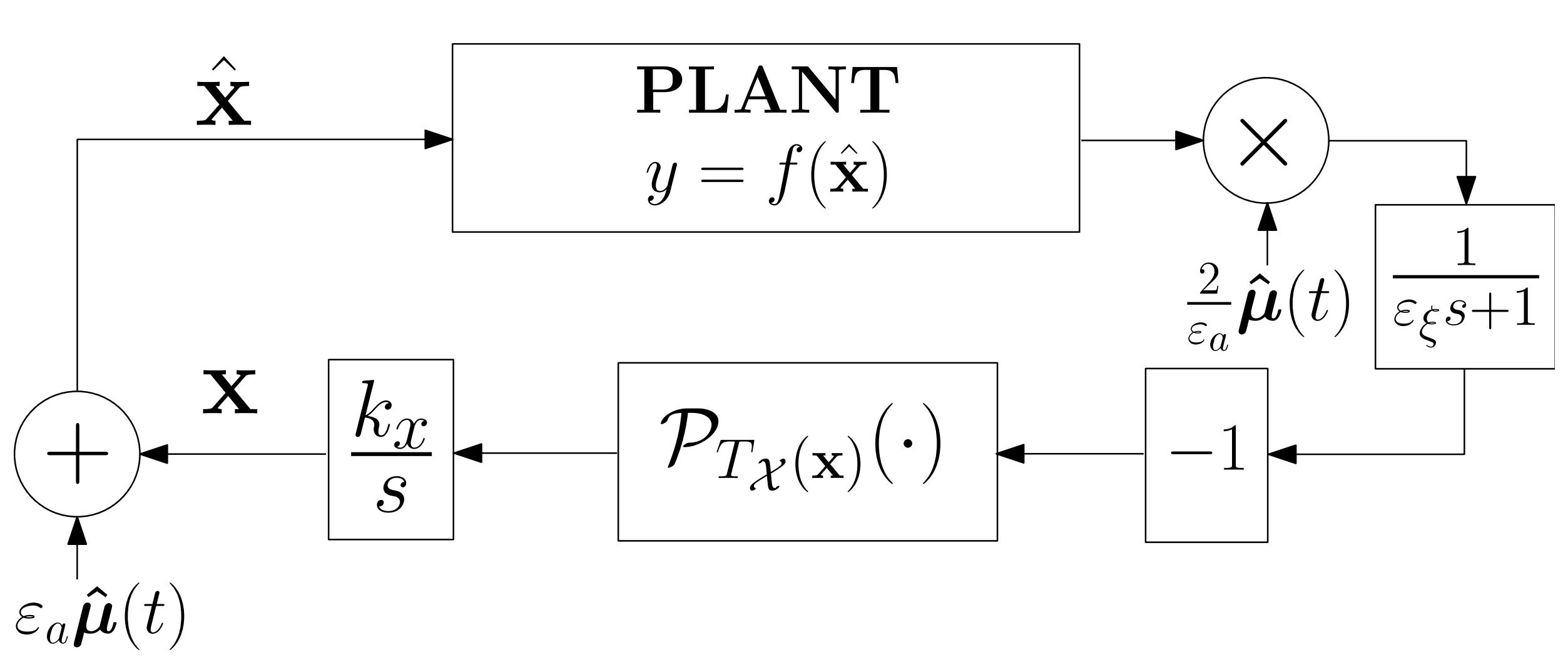
Figure 5: Block diagram of the DP-GZO algorithm.

The existence of solutions for the Krasovskii regularization of (35) is guaranteed by well-posedness of (36) and standard viability results [50, Theorems 3.3.4, 3.3.5]. Moreover, it can be shown that system (36) accurately captures the limiting behavior of (35) under arbitrarily small additive perturbations on the states and dynamics via the so-called Hermes solutions [36, Chapter 4]. This suggests that (36) provides a useful characterization of the solutions of the ODE $\dot{\mathbf{z}}=\mathbf{h}(\mathbf{z})$ under small perturbations, a setting that naturally emerges in the context of ZO dynamics.

The solutions of (35) are also solutions of its Krasovskii regularization, but the converse is not always true. However, under mild regularity assumptions on (35), it turns out that every solution of its Krasovskii regularization is also a standard (i.e., Caratheodory) solution of (35) [1]. This fact allows us to study the behaviors of the DP-GZO dynamics (35) based on its nominal target system:

$$\dot{\mathbf{p}}=k_{x}\cdot\mathcal{P}_{T_{\mathcal{X}}(\mathbf{p})}(-\nabla f(\mathbf{p})).$$ (37)

The following theorem establishes the stability and (practical) safety properties for the DP-GZO dynamics (35). The proof of Theorem 5 is provided in Section VI-E.

Theorem 5.

Suppose that Assumptions 1-3 hold and that $f$ is strictly convex. Then, for any $\Delta>\nu>0$, there exists $\hat{\varepsilon}_{\xi}>0$ such that for all $\varepsilon_{\xi}\in(0,\hat{\varepsilon}_{\xi})$, there exists $\hat{\varepsilon}_{a}>0$ such that for all $\varepsilon_{a}\in(0,\hat{\varepsilon}_{a})$, there exists $\hat{\varepsilon}_{\omega}>0$ such that for all $\varepsilon_{\omega}\in(0,\hat{\varepsilon}_{\omega})$, every solution $\mathbf{z}(t)$ of the DP-ZO dynamics (35) with $\mathbf{z}(0)\in\mathbf{C}_{1}\cap\left(\mathcal{W}_{1}^{*}+\Delta\mathbb{B}\right)\times\mathbb{T}^{n})$ is complete and satisfies the Practical Convergence property (18) and the Practical Safety property (19). $\square$

Although the results of Theorem 5 for the DP-GZO dynamics (35) are similar to Theorem 1 for the P-GZO dynamics (10), their analyses and proof ideas are different, as the DP-ZO dynamics are discontinuous; see Section VI-E.

Remark 5.

With sufficiently small parameters $\varepsilon_{a},\varepsilon_{\xi},\varepsilon_{\omega}$, the $\mathbf{x}$-trajectories of the DP-GZO dynamics (35) emulate the trajectories of (37). Since any closed and convex set $\mathcal{X}\subset\mathbb{R}^{n}$ is Clarke regular [1, Definition 2.2] and prox-regular [1, Definition 6.1], and since $f$ is locally Lipschitz under Assumption 1, the solutions of (35) and its Krasovskii regularization coincide and are unique [51, Thm. 4.2]. Nevertheless, since the uniqueness of solutions is not required in our analysis, the convexity of $\mathcal{X}$ and the strict convexity of $f$ can be relaxed to mere Clarke regularity and the assumption that all first-order critical points of (8) are optimal and also equilibria of (37). $\square$

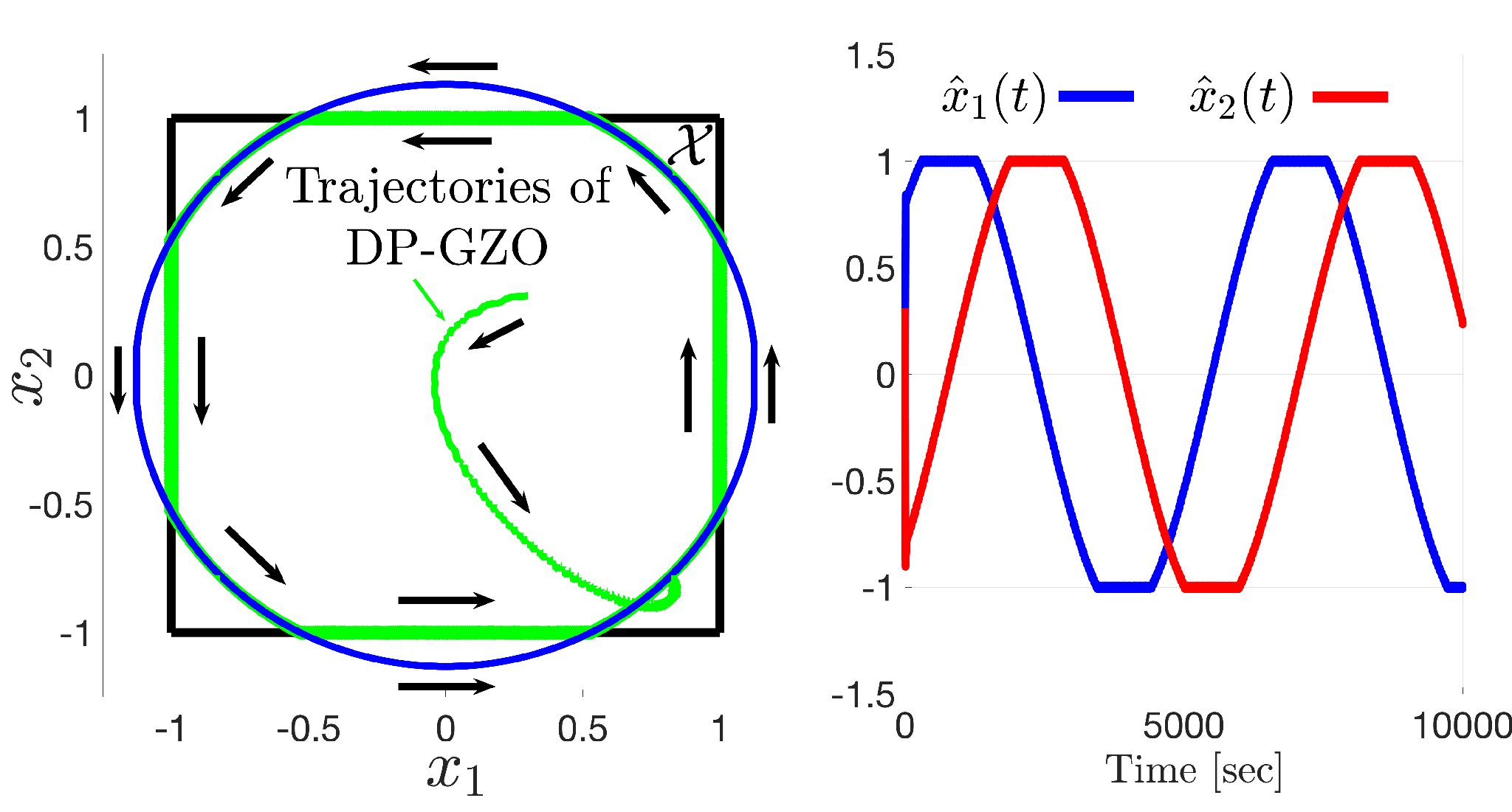
Figure 6: Illustration of the DP-GZO (35) restricted to a box $\mathcal{X}=[-1,1]\times[-1,1]$, with a slowly time-varying minimizer of $f$ corresponding to the blue circle trajectory.

Example 2.

To illustrate the behavior of system (35), we consider a simple example of problem (9), where the feasible set $\mathcal{X}:=[-1,1]\times[-1,1]$ is a box constraint and the objective function $f$ is the same as the one in Example 1, but now with $\dot{\theta}_{1}=-\varepsilon_{p}\theta_{2}$ and $\dot{\theta}_{2}=\varepsilon_{p}\theta_{1}$, $\varepsilon_{p}=1\times 10^{-3}$. As shown in Figure 6, this exosystem makes the the minimizer of $f$ in $\mathbb{R}^{n}$ (i.e., $\arg\min_{\mathbf{x}}f(\mathbf{x})$) a slowly varying signal that forms a circular trajectory, shown in blue color. It can be observed that the trajectory $t\mapsto\mathbf{x}(t)$, shown in green, generated by the DP-GZO dynamics (35) tends to closely track the blue minimizer trajectory, but it stays in the feasible set at all times due to the projection map. Similar to Example 1, we have replaced $\mathcal{X}$ with a shrunk set $\hat{\mathcal{X}}_{\varepsilon_{a}}:=[-1+\varepsilon_{a},1-\varepsilon_{a}]\times[-1+\varepsilon_{a},1-\varepsilon_{a}]$ in (35a) to ensure the actual input $\hat{\mathbf{x}}\in\mathcal{X}$ all the time. Here, $\varepsilon_{a}=1\times 10^{-2}$, so the difference between $\hat{\mathcal{X}}_{\varepsilon_{a}}$ and $\mathcal{X}$ is almost indistinguishable. The right plot shows the trajectory of each of the components of $\hat{\mathbf{x}}$. $\square$

V-B Structural Robustness

The ZO algorithms proposed in this paper rely heavily on function evaluations (or system output measurements) to steer the decision variable $\hat{\mathbf{x}}$ to an optimal solution of problem (8) or (9). Hence, suitable robustness properties are necessary to handle small disturbances and noises that are inevitable in practice. The following result, i.e., Corollary 1, indicates that, under the corresponding assumptions of Theorems 1-5, all the proposed ZO algorithms (10), (30), (35) are structurally robust to small bounded additive perturbations on the states and dynamics. We rewrite these ZO dynamics as $\mathbf{z}\in\mathbf{C},\dot{\mathbf{z}}=\mathbf{h}(\mathbf{z})$, and consider their perturbed dynamics (38):

$$\mathbf{z}+\mathbf{e}\in\mathbf{C},~{}~{}~{}\dot{\mathbf{z}}=\mathbf{h}(\mathbf{z}+\mathbf{e})+\mathbf{e},$$ (38)

where $\mathbf{z}$ is the state of the ZO dynamics, $\mathbf{h}(\cdot)$ denotes the vector field describing the right-hand side of the dynamics, $\mathbf{e}$ is the additive noise, and $\mathbf{C}$ denotes the flow set.

Corollary 1.

Under the assumptions and parameters of Theorems 1-5, there exists $\bar{e}>0$ such that for any additive noise $\mathbf{e}(t):[0,+\infty)\!\to\!\mathbb{R}^{n}$ with $\sup_{t\geq 0}||\mathbf{e}(t)||\leq\bar{e}$, the trajectory $\mathbf{z}(t)$ of the perturbed ZO dynamics (38) satisfies the respective practical convergence bounds in Theorems 1-5. $\square$

The result is a corollary of Theorems 1-5 because the convergence, well-posedness, and stability properties of the dynamics imply that, for each sufficiently large compact set of initial conditions $K$, and fixed parameters of the controller that induce the convergence bounds (which are actually uniform, see Section VI), there exists a compact set that is locally asymptotically stable under the nominal dynamics (the so-called Omega-limit set of $K$), and also semi-globally practical asymptotically stable as $\bar{e}\to 0^{+}$ for the perturbed system (38) [36, Chapter 7]. However, we note that Corollary 1 only shows the existence of a sufficiently small $\bar{e}$, such that any additive noise bounded by $\bar{e}$ does not change drastically the convergence properties of the ZO algorithms. However, in practice, the computation of this robustness bound is important, but difficult and application-dependent.

VI ANALYSIS AND PROOFS

In this section, we present the proofs of our main results. Since the result of Theorem 1 can be seen as a particular case of Theorem 4 when the set of inequality constraints (8c) is empty, we first present the proof of Theorem 4. Subsequently, we show how to adapt this proof to Theorem 1. The proofs of Theorems 2, 3, 5 are based on the construction of suitable Lyapunov functions, and therefore are presented afterwards.

VI-A Proof of Theorem 4

Let $\mathbf{y}:=[\mathbf{x};\bm{\lambda}]$, $\bm{\xi}:=[\bm{\xi}_{1};\bm{\xi}_{2}]$, and $\mathbf{s}:=[\mathbf{y};\bm{\xi}]$. The P-PDZO dynamics (30a)-(30d) can be written in compact form as

$$\dot{\mathbf{s}}=\begin{bmatrix}\dot{\mathbf{y}}\\ \dot{\bm{\xi}}\end{bmatrix}=\begin{bmatrix}\mathbf{q}_{1}(\mathbf{y},\bm{\xi})\\ \frac{1}{\varepsilon_{\xi}}(-\bm{\xi}+\mathbf{q}_{2}(\mathbf{y},\bm{\mu}))\end{bmatrix}:=\mathbf{q}(\mathbf{s},\bm{\mu}),$$ (39)

where $\mathbf{q}_{1}$ captures the dynamics (30a) and $\mathbf{q}_{2}$ is given by

$$\mathbf{q}_{2}(\mathbf{y},\bm{\mu}):=\begin{bmatrix}\frac{2}{\varepsilon_{a}}\big{(}f(\hat{\mathbf{x}})+\bm{\lambda}^{\top}\mathbf{g}(\hat{\mathbf{x}})\big{)}\hat{\bm{\mu}}\\ \mathbf{g}(\hat{\mathbf{x}})\end{bmatrix},$$ (40)

where $\bm{\mu}$ is generated by the oscillator (30e), and $\hat{\mathbf{x}},\hat{\bm{\mu}}$ are defined in (11) and (12). We analyze the stability properties of this system using multi-time scale techniques based on averaging theory and singular perturbation theory. We divide the analysis into the following three main steps.

Step 1) Behavior of system (39) restricted to compact sets: Let $\Delta>0$ and $\mathcal{Y}:=\mathcal{X}\times\mathbb{R}^{m}_{+}$. Consider the compact set $[(\mathcal{Y}^{*}+\Delta\mathbb{B})\cap\mathcal{Y}]\times\Delta\mathbb{B}$ for the initial condition $\mathbf{s}(0)$ and any desired $\Delta>0$. Here, $\mathcal{Y}^{*}+\Delta\mathbb{B}$ denotes the union of all sets obtained by taking a closed ball of radius $\Delta$ around each point in the saddle point set $\mathcal{Y}^{*}$.

By items (a)-(c) in Theorem 4, the compact set $\mathcal{Y}^{*}$ is uniformly globally asymptotically stable (UGAS) for the model-based dynamics (32) restricted to evolve in $\mathcal{Y}$, which is also a forward invariant set. Thus, there exists a class-$\mathcal{KL}$ function $\beta$ such that for any initial condition $\mathbf{p}(0)\in\mathcal{Y}$, the solutions $\mathbf{p}$ of (32) satisfy $||\mathbf{p}(t)||_{\mathcal{Y}^{*}}\leq\beta(||\mathbf{p}(0)||_{\mathcal{Y}^{*}},\,t)$ for all $t\geq 0$. Without loss of generality, let $\nu\in(0,1)$ and consider the set

$$\mathcal{F}\!:=\!\Big{\{}\mathbf{y}\!\in\!\mathcal{Y}:||\mathbf{y}||_{\mathcal{Y}^{*}}\leq\beta\big{(}\max_{\mathbf{v}\in\mathcal{Y}^{*}+\Delta\mathbb{B}}||\mathbf{v}||_{\mathcal{Y}^{*}},\,0\big{)}+1\Big{\}}.$$ (41)

Note that the set $\mathcal{F}$ is compact under the assumption that $\mathcal{Y}^{*}$ is compact. Due to the boundedness of $\mathcal{F}$, there exists a positive constant $M_{1}$ such that $\mathcal{F}\subset M_{1}\mathbb{B}$. Let

$$\bm{\ell}(\mathbf{y})\!:=\!\begin{bmatrix}\nabla f(\mathbf{x})+\sum_{j=1}^{m}\lambda_{j}\nabla g_{j}(\mathbf{x})\\ \mathbf{g}(\mathbf{x})\end{bmatrix},$$ (42)

and note that, by continuity of $\bm{\ell}$, there exists a positive constant $M_{2}>\max\{\Delta,1\}$ such that $||\bm{\ell}(\mathbf{y})||+1\leq M_{2}$ for all $||\mathbf{y}||\leq M_{1}$. Denote $M_{3}=M_{2}+1$. We then study the behavior of system (39) restricted to evolve in the compact set $\mathcal{F}\times M_{3}\mathbb{B}$.

Step 2) Stability properties of the average dynamics of system (39): Since the solutions of the oscillator (30e) are given by (14), and $\mu_{i}(0)^{2}+\mu_{i+1}(0)^{2}=1$ for all $i\in\{1,3,\ldots,2n-1\}$, system (39) with small values of $\varepsilon_{\omega}$ is in standard form for the application of averaging theory along the trajectories of $\bm{\mu}$. The following Lemma 3 characterizes the average map of $\mathbf{q}_{2}$. The proof is presented in Appendix A-B.

Lemma 3.

The average of $t\mapsto\mathbf{q}_{2}(\mathbf{y},\bm{\mu}(t))$ is given by

$$\bar{\mathbf{q}}_{2}(\mathbf{y}):= \frac{1}{T}\!\int_{0}^{T}\!\mathbf{q}_{2}(\mathbf{y},\bm{\mu}(t))\,dt=\bm{\ell}(\mathbf{y})+\mathcal{O}(\varepsilon_{a}),$$ (43)

where $T$ is the common period of $\bm{\mu}$. $\square$

Using Lemma 3, we obtain the average dynamics of (39):

$$\dot{\bar{\mathbf{s}}}=\!\begin{bmatrix}\dot{\bar{\mathbf{y}}}\\ \dot{\bar{\bm{\xi}}}\end{bmatrix}\!=\!\begin{bmatrix}\mathbf{q}_{1}(\bar{\mathbf{y}},\bar{\bm{\xi}})\\ \frac{1}{\varepsilon_{\xi}}(-\bar{\bm{\xi}}+\bm{\ell}(\bar{\mathbf{y}})+\mathcal{O}(\varepsilon_{a}))\end{bmatrix},$$ (44)

where $\bar{\mathbf{s}}:=[\bar{\mathbf{y}};\bar{\bm{\xi}}]$. We study (44) restricted to evolve in the compact set $\mathcal{F}\times M_{3}\mathbb{B}$. We treat the right-hand side of (44) as an $\mathcal{O}(\varepsilon_{a})$-perturbation of a nominal system with $\varepsilon_{a}=0$. This nominal system (i.e., (44) with $\varepsilon_{a}=0$) is in the standard form for the application of singular perturbation theory [38], with $\bar{\mathbf{y}}$ being the slow state, and $\bar{\bm{\xi}}$ being the fast state. The boundary layer dynamics of this nominal system, in the time scale $\tau=t/\varepsilon_{\xi}$, are

$$\frac{d\bar{\bm{\xi}}}{d\tau}=-\,\bar{\bm{\xi}}+\bm{\ell}(\bar{\mathbf{y}}),$$ (45)

where $\bar{\mathbf{y}}$ is kept constant. This linear system (45) has a unique exponentially stable equilibrium point $\bar{\bm{\xi}}^{*}=\bm{\ell}(\bar{\mathbf{y}})$. As a result, the associated reduced system is derived as

$$\dot{\bar{\mathbf{y}}}=\mathbf{q}_{1}(\bar{\mathbf{y}},\,\bm{\ell}(\bar{\mathbf{y}})),$$ (46)

which is exactly the nominal target system (32). Under the assumptions of Theorem 4, system (46) renders the set $\mathcal{Y}^{*}$ UGAS. By using singular perturbation theory [52, Theorem 2], we can conclude that, as $\varepsilon_{\xi}\to 0^{+}$, the set $\mathcal{Y}^{*}\times{M}_{3}\mathbb{B}$ is semi-globally practically asymptotically stable (SGPAS) for the unperturbed average system (44) with $\varepsilon_{a}=0$. Since system (44) has a continuous right-hand side , the perturbed average system (44) also renders the set $\mathcal{Y}^{*}\times{M}_{3}\mathbb{B}$ SGPAS as $(\varepsilon_{\xi},\varepsilon_{a})\to 0^{+}$, which is stated as Lemma 4.

Lemma 4.

There exists $\beta\in\mathcal{K}\mathcal{L}$ such that for each $\nu>0$, there exists $\hat{\varepsilon}_{\xi}>0$ such that for any $\varepsilon_{\xi}\in(0,\hat{\varepsilon}_{\xi})$, there exists $\hat{\varepsilon}_{a}>0$ such that for any $\varepsilon_{a}\in(0,\hat{\varepsilon}_{a})$, every solution $\bar{\mathbf{s}}$ of the average system (44) (restricted in $\mathcal{F}\times M_{3}\mathbb{B}$) with initial condition $\bar{\mathbf{s}}(0)\in[(\mathcal{Y}^{*}\!+\!\Delta\mathbb{B})\cap\mathcal{Y}]\!\times\!\Delta\mathbb{B}$ satisfies

$$||\bar{\mathbf{y}}(t)||_{\mathcal{Y}^{*}}\!\leq\beta(||\bar{\mathbf{y}}(0)||_{\mathcal{Y}^{*}},\,t)+\frac{\nu}{4},$$ (47)

for all $t\in\mathrm{dom}(\bar{\mathbf{s}})$. $\square$

Since the average system (44) is restricted in $\mathcal{F}\times M_{3}\mathbb{B}$, we have $||\bar{\bm{\xi}}(t)||_{M_{3}\mathbb{B}}=0$ for all $t\in\mathrm{dom}(\bar{\mathbf{s}})$, which implies that $||\bar{\mathbf{s}}(t)||_{\mathcal{Y}^{*}\times M_{3}\mathbb{B}}=||\bar{\mathbf{y}}(t)||_{\mathcal{Y}^{*}}$ for all $t\in\mathrm{dom}(\bar{\mathbf{s}})$. Hence, it follows that for all $t\in\mathrm{dom}(\bar{\mathbf{s}})$:

$$||\bar{\mathbf{s}}(t)||_{\mathcal{Y}^{*}\times M_{3}\mathbb{B}}\leq\beta(||\bar{\mathbf{s}}(0)||_{\mathcal{Y}^{*}\times M_{3}\mathbb{B}},\,t)+\frac{\nu}{4}.$$

Next, we show the completeness of solutions of the average system (44) by leveraging Lemma 5, which follows as a special case of [53, Lemma 5].

Lemma 5.

Let $k,M_{2}>0$ be given and $\mathbf{u}:\mathbb{R}_{+}\to M_{2}\mathbb{B}$ be a continuous function of time. Then, the set $M_{2}\mathbb{B}$ is forward invariant under the dynamics $\dot{\bm{\xi}}=k\cdot(-\bm{\xi}+\mathbf{u}(t))$. $\square$

Under the initial condition $\bar{\mathbf{s}}(0)\in[(\mathcal{Y}^{*}\!+\!\Delta\mathbb{B})\cap\mathcal{Y}]\!\times\!\Delta\mathbb{B}$, by (47), the trajectory $\bar{\mathbf{y}}$ of (44) satisfies $\bar{\mathbf{y}}(t)\in\mathrm{int}(\mathcal{F})$ for all $t\in\mathrm{dom}(\bar{\mathbf{s}})$. This implies that $||\bar{\mathbf{y}}(t)||\leq M_{1}$ and thus $||\bm{\ell}(\bar{\mathbf{y}}(t))\!+\!\mathcal{O}(\epsilon_{a}))||<M_{2}$ for all $t\in\mathrm{dom}(\bar{\mathbf{s}})$, where we take $||\mathcal{O}(\epsilon_{a})||<1$ for all $\varepsilon_{a}\in(0,\hat{\varepsilon}_{a})$ without loss of generality. Using Lemma 5, $\bar{\bm{\xi}}(t)\in M_{2}\mathbb{B}\subset\mathrm{int}(M_{3}\mathbb{B})$ for all $t\geq 0$. Thus, under the given initialization, $\bar{\mathbf{s}}$ satisfies

$$\bar{\mathbf{s}}(t)\in\mathrm{int}(\mathcal{F}\times M_{3}\mathbb{B}),\quad\forall t\geq t_{0},$$ (48)

and thus it has an unbounded time domain. The following lemma proved in Appendix A-C will be useful for our results.

Lemma 6.

There exists $\hat{\varepsilon}_{\xi}>0$ such that for any $\varepsilon_{\xi}\in(0,\hat{\varepsilon}_{\xi})$, there exists $\hat{\varepsilon}_{a}>0$ such that for any $\varepsilon_{a}\in(0,\hat{\varepsilon}_{a})$, there exists a compact set $\Omega(\mathcal{F}\times M_{3}\mathbb{B})$ that is uniformly globally (pre)-asymptotically stable for the average system (44) restricted to $\mathcal{F}\times M_{3}\mathbb{B}$. $\square$

Step 3) Link the stability property of the average dynamics (44) to the stability property of the original system (39): Since the set $\mathcal{Y}^{*}\times M_{3}\mathbb{B}$ is SGPAS for the average system (44) (restricted in $\mathcal{F}\times M_{3}\mathbb{B}$) as $(\varepsilon_{\xi},\varepsilon_{a})\to 0^{+}$, by averaging theory for perturbed systems [30, Theorem 7], it follows that for each pair of $(\varepsilon_{\xi},\varepsilon_{a})$ inducing the bound (47), there exists $\hat{\varepsilon}_{\omega}>0$ such that for any $\varepsilon_{\omega}\in(0,\hat{\varepsilon}_{\omega})$, the solution $\mathbf{s}$ of the original system (39) (restricted to $\mathcal{F}\times M_{3}\mathbb{B}$) satisfies

$$||\mathbf{s}(t)||_{\mathcal{Y}^{*}\times M_{3}\mathbb{B}}\leq\beta(||\mathbf{s}(0)||_{\mathcal{Y}^{*}\times M_{3}\mathbb{B}},\,t)+\nu,$$ (49)

for all $t\in\mathrm{dom}(\mathbf{s})$. Since $||\mathbf{x}(t)||_{\mathcal{Y}^{*}}=||\mathbf{s}(t)||_{\mathcal{Y}^{*}\times M_{3}\mathbb{B}}$ for all $t\in\mathrm{dom}(\mathbf{s})$, we obtain the bound (33). The only task left is to show the completeness of solutions of the original system (39). This can be done by using the following lemma, corresponding to [52, Theorem 1].

Lemma 7.

Let $(\varepsilon_{\xi},\varepsilon_{a})>0$ take sufficiently small values such that Lemmas 4 and 6 hold. Then, for each $\tilde{T},\delta>0$, there exists $\hat{\varepsilon}_{\omega}>0$ such that for all $\varepsilon_{\omega}\in(0,\hat{\varepsilon}_{\omega})$ and all solutions $\mathbf{s}$ of the original system (39), with $\mathbf{s}(0)\in[(\mathcal{Y}^{*}+\Delta\mathbb{B})\cap\mathcal{Y}]\times\Delta\mathbb{B}$, there exists a solution $\bar{\mathbf{s}}$ of the average system (44), with $\bar{\mathbf{s}}(0)\in[(\mathcal{Y}^{*}+\Delta\mathbb{B})\cap\mathcal{Y}]\times\Delta\mathbb{B}$ such that $\mathbf{s}$ and $\bar{\mathbf{s}}$ are $(\tau,\varepsilon)$ close. $\square$

By Lemma 6, there exists a $\mathcal{KL}$-class function $\tilde{\beta}$ such that every solution of the average system (44) satisfies

$$||\bar{\mathbf{s}}(t)||_{\Omega(\mathcal{F}\times M_{3}\mathbb{B})}\leq\tilde{\beta}(||\bar{\mathbf{s}}(0)||_{\Omega(\mathcal{F}\times M_{3}\mathbb{B})},t),$$ (50)

for all $t\in\mathrm{dom}(\bar{\mathbf{s}})$. Moreover, by (48), the trajectories $\bar{\mathbf{s}}$ are complete if $\bar{\mathbf{s}}(0)\in[(\mathcal{Y}^{*}\!+\!\Delta\mathbb{B})\cap\mathcal{Y}]\!\times\!\Delta\mathbb{B}$. Using this bound, the closeness of solutions property of Lemma 7, and stability results in averaging theory [52, Theorem 2], there exists $\hat{\varepsilon}_{\omega}$ such that for all $\varepsilon_{\omega}\in(0,\hat{\varepsilon}_{\omega})$, every solution of the original system (39) with $\mathbf{s}(0)\in[(\mathcal{Y}^{*}\!+\!\Delta\mathbb{B})\cap\mathcal{Y}]\!\times\!\Delta\mathbb{B}$, satisfies

$$||{\mathbf{s}}(t)||_{\Omega(\mathcal{F}\times M_{3}\mathbb{B})}\leq\tilde{\beta}(||{\mathbf{s}}(0)||_{\Omega(\mathcal{F}\times M_{3}\mathbb{B})},t)+\frac{\nu}{2},$$ (51)

for all $t\in\text{dom}(\mathbf{s})$. This implies that $\mathbf{s}(t)\in\mathrm{int}(\mathcal{F}\times M_{3}\mathbb{B})$ for all $t\geq 0$. Therefore, every solution $\mathbf{s}$ of the original system (39), under the given initialization, has an unbounded time domain. Thus Theorem 4 is proved.

VI-B Proof of Theorem 1

The proof of Theorem 1 follows the same steps as the proof of Theorem 4. In this case, $\mathbf{q}_{2}:=\frac{2}{\varepsilon_{a}}f(\hat{\mathbf{x}})\hat{\bm{\mu}}$, and the function $\bm{\ell}(\cdot)$ in (44) becomes $\bm{\ell}(\mathbf{x})=\nabla f(\mathbf{x})$. Therefore, system (46) is precisely the Lipschitz continuous projected gradient flow (17). Under the conditions (a) and (b) in Theorem 1, there exists a class $\mathcal{K}\mathcal{L}$ function $\beta$ such that Lemma 6 holds. The rest proof follows the same steps as the proof of Theorem 4.

VI-C Proof of Theorem 2

Following similar computations to those in Lemma 3, we compute the average dynamics of (10) along the trajectories of $\bm{\mu}$ and obtain:

$$\dot{\bar{\mathbf{x}}} =k_{x}\mathcal{P}_{\mathcal{X}}\left(\mathbf{\bar{x}}-\alpha_{x}\bar{\bm{\xi}}\right)-k_{x}\mathbf{\bar{x}},$$ (52a)

$$\dot{\mathbf{\bar{\bm{\xi}}}} =\frac{1}{\varepsilon_{\xi}}\left(-{\bar{\bm{\xi}}}+\nabla_{\bar{\mathbf{x}}}f(\mathbf{\bar{x}},\bar{\bm{\theta}})+\mathcal{O}(\varepsilon_{a})\right),$$ (52b)

$$\dot{\bar{\bm{\theta}}} =\varepsilon_{\theta}\Pi(\bar{\bm{\theta}}),$$ (52c)

which is restricted to evolve in the set $\mathbf{C}_{3}:=\mathcal{X}\times\mathbb{R}^{n}\times\Theta$. Next, we establish a key lemma for the average system (52).

Lemma 8.

For system (52) with $\varepsilon_{a}=0$ and $\varepsilon_{\theta}>0$, there exist $\hat{\alpha}_{x},\hat{k}_{x},\hat{\varepsilon}_{\xi}>0$, such that for all $\alpha_{x}\in(0,\hat{\alpha}_{x})$, all $k_{x}\in(0,\hat{k}_{x})$ and all $\varepsilon_{\xi}\in(0,\hat{\varepsilon}_{\xi})$, every solution satisfies

$$||{\bar{\mathbf{s}}}(t)-{\mathbf{s}}^{*}(\bar{\bm{\theta}}(t))||\leq c_{1}||{\bar{\mathbf{s}}}(0) -{\mathbf{s}}^{*}(\bar{\bm{\theta}}(0))||e^{-c_{2}t}$$

$$\qquad+c\sup_{0\leq\tau\leq t}||\dot{\bar{\bm{\theta}}}(\tau)||,$$

where $\mathbf{\bar{s}}:=(\mathbf{\bar{x}},{\bar{\bm{\xi}}})$, $\mathbf{s}^{*}(\bar{\bm{\theta}}):=(\mathbf{x}^{*}(\bar{\bm{\theta}}),\nabla_{\mathbf{x}}f(\mathbf{x}^{*}(\bar{\bm{\theta}}),\bar{\bm{\theta}}))$, and $c_{1},c_{2},c>0$. $\square$

Proof: We introduce the error variables $\tilde{\mathbf{x}}:=\mathbf{\bar{x}}-\mathbf{x}^{*}(\bar{\bm{\theta}})$ and $\tilde{\bm{\xi}}:=\mathbf{\bar{\bm{\xi}}}-\nabla_{\mathbf{x}}f(\tilde{\mathbf{x}}+\mathbf{x}^{*},\mathbf{\bar{\bm{\theta}}})$, which leads to the error dynamics

$$\dot{\tilde{\mathbf{x}}} =k_{x}\mathcal{P}_{\mathcal{X}}\left(\tilde{\mathbf{x}}+\mathbf{x}^{*}-\alpha_{x}(\tilde{\bm{\xi}}+\nabla_{\mathbf{x}}f(\mathbf{\tilde{x}}+\mathbf{x}^{*},\bar{\bm{\theta}}))\right)$$

$$~{}~{}~{}-k_{x}(\tilde{\mathbf{x}}+\mathbf{x}^{*})-\dot{\mathbf{x}}^{*},$$ (53a)

$$\dot{\tilde{\bm{\xi}}} =-\frac{1}{\varepsilon_{\xi}}\tilde{\bm{\xi}}-\frac{d}{dt}\nabla_{\mathbf{x}}f(\tilde{\mathbf{x}}+\mathbf{x}^{*},\bar{\bm{\theta}}).$$ (53b)

We study the stability properties of (53) with respect to the origin. To this end, we consider the Lyapunov function:

$$W(\tilde{\mathbf{x}},\tilde{\bm{\xi}})=(1-\lambda)V_{x}(\tilde{\mathbf{x}})+\lambda V_{\xi}(\tilde{\bm{\xi}}),$$ (54)

where $\lambda\in(0,1)$, $V_{x}(\tilde{\mathbf{x}})=\frac{1}{2}||\tilde{\mathbf{x}}|||^{2}$ and $V_{\xi}(\tilde{\bm{\xi}})=\frac{1}{2}||\tilde{\bm{\xi}}||^{2}$. The function (54) is radially unbounded and positive definite, and it satisfies $\dot{W}=(1-\lambda)\tilde{\mathbf{x}}^{\top}\dot{\tilde{\mathbf{x}}}+\lambda\tilde{\bm{\xi}}^{\top}\dot{\tilde{\bm{\xi}}}$. Let $\mathbf{h}(\bar{\bm{\theta}},\tilde{\mathbf{x}}):=\nabla_{\mathbf{x}}f(\tilde{\mathbf{x}}+\mathbf{x}^{*},\bar{\bm{\theta}})$ and thus $\bar{\bm{\xi}}=\tilde{\bm{\xi}}+\mathbf{h}(\bar{\bm{\theta}},\tilde{\mathbf{x}})$. We rewrite the $\tilde{\mathbf{x}}$-error dynamics (53a) compactly as

$$\dot{\tilde{\mathbf{x}}}=\mathbf{f}_{x}(\tilde{\mathbf{x}},\tilde{\bm{\xi}}+\mathbf{h}(\bar{\bm{\theta}},\tilde{\mathbf{x}}))-\dot{\mathbf{x}}^{*}.$$ (55)

It follows that

$$\tilde{\mathbf{x}}^{\top}\dot{\tilde{\mathbf{x}}}=\tilde{\mathbf{x}}^{\top}(\mathbf{f}_{x}(\tilde{\mathbf{x}},\tilde{\bm{\xi}}+\mathbf{h}(\bar{\bm{\theta}},\tilde{\mathbf{x}}))-\dot{\mathbf{x}}^{*})$$

$$= \tilde{\mathbf{x}}^{\top}(\mathbf{f}_{x}(\tilde{\mathbf{x}},\tilde{\bm{\xi}}+\mathbf{h}(\bar{\bm{\theta}},\tilde{\mathbf{x}}))-\mathbf{f}_{x}(\tilde{\mathbf{x}},\mathbf{h}(\bar{\bm{\theta}},\tilde{\mathbf{x}})))$$

$$~{}~{}~{}+\tilde{\mathbf{x}}^{\top}\left(\mathbf{f}_{x}(\tilde{\mathbf{x}},\mathbf{h}(\bar{\bm{\theta}},\tilde{\mathbf{x}}))-\dot{\mathbf{x}}^{*}\right)$$

$$\leq ||\tilde{\mathbf{x}}||\cdot||\dot{\mathbf{x}}^{*}||+||\tilde{\mathbf{x}}||\cdot||\mathbf{f}_{x}(\tilde{\mathbf{x}},\tilde{\bm{\xi}}+\mathbf{h}(\bar{\bm{\theta}},\tilde{\mathbf{x}}))-\mathbf{f}_{x}(\tilde{\mathbf{x}},\mathbf{h}(\bar{\bm{\theta}},\tilde{\mathbf{x}}))||$$

$$~{}~{}~{}+\tilde{\mathbf{x}}^{\top}\mathbf{f}_{x}(\tilde{\mathbf{x}},\mathbf{h}(\bar{\bm{\theta}},\tilde{\mathbf{x}}))$$

$$\leq ||\tilde{\mathbf{x}}||\cdot||\dot{\mathbf{x}}^{*}||+k_{x}\alpha_{x}||\tilde{\mathbf{x}}||\cdot||\tilde{\bm{\xi}}||+\tilde{\mathbf{x}}^{\top}\mathbf{f}_{x}(\tilde{\mathbf{x}},\mathbf{h}(\bar{\bm{\theta}},\tilde{\mathbf{x}})),$$ (56)

where we use the fact that $\mathcal{P}_{\mathcal{X}}(\cdot)$ is Lipschitz continuous with unitary Lipschitz constant [54, Proposition 2.4.1], such that:

$$\ ||\mathbf{f}_{x}(\tilde{\mathbf{x}},\bar{\bm{\xi}})-\mathbf{f}_{x}(\tilde{\mathbf{x}},\mathbf{h}(\bar{\bm{\theta}},\tilde{\mathbf{x}}))||$$

$$\leq \ k_{x}\alpha_{x}||\bar{\bm{\xi}}-h(\bar{\bm{\theta}},\mathbf{x})||=k_{x}\alpha_{x}||\tilde{\bm{\xi}}||.$$ (57)

Using the uniform strong convexity and Lipschitz properties of Assumption 4 and the same steps of the proof of [34, Theorem 4], we obtain

$$\tilde{\mathbf{x}}^{\top}\mathbf{f}_{x}(\tilde{\mathbf{x}},\mathbf{h}(\bar{\bm{\theta}},\tilde{\mathbf{x}}))\leq-\tilde{k}_{x}||\tilde{\mathbf{x}}||^{2},$$

where $\tilde{k}_{x}=\alpha_{x}(\gamma-\frac{\alpha_{x}\ell^{2}}{4})$. Thus, for all $\alpha_{x}\in(0,\hat{\alpha}_{x})$ with $\hat{\alpha}_{x}=\frac{4\gamma}{\ell^{2}}$ such that $\tilde{k}_{x}$ is positive, we obtain

$$\tilde{\mathbf{x}}^{\top}\dot{\tilde{\mathbf{x}}}\leq-\tilde{k}_{x}||\tilde{\mathbf{x}}||^{2}+k_{x}\alpha_{x}||\tilde{\mathbf{x}}||\cdot||\tilde{\bm{\xi}}||+m||\tilde{\mathbf{x}}||\cdot||\dot{\bm{\theta}}||,$$ (58)

where $m:=\max_{\bar{\bm{\theta}}\in\Theta}||\nabla\mathbf{d}(\bar{\bm{\theta}})||$ and $\mathbf{d}(\cdot)$ is defined in (21). Note that $m<\infty$ because $\Theta$ is compact and $\mathbf{d}$ is continuously differentiable by Assumption 4. From (53), we have

$$\tilde{\bm{\xi}}^{\top}\dot{\tilde{\bm{\xi}}}=-\frac{1}{\varepsilon_{\xi}}||\tilde{\bm{\xi}}||^{2}-\tilde{\bm{\xi}}^{\top}\frac{d}{dt}\nabla_{\mathbf{x}}f(\tilde{\mathbf{x}}+\mathbf{x}^{*},\bm{\theta}),$$

and note that

$$\frac{d}{dt}\nabla_{\mathbf{x}}f(\tilde{\mathbf{x}}+\mathbf{x}^{*},\bm{\theta}) =H_{f}(\bar{\bm{\theta}},\tilde{\mathbf{x}}+\mathbf{x}^{*})(\dot{\tilde{\mathbf{x}}}+\dot{\mathbf{x}}^{*})$$

$$+\frac{\partial}{\partial\bm{\theta}}\nabla_{\mathbf{x}}f(\tilde{\mathbf{x}}+\mathbf{x}^{*},\bm{\theta})\dot{\bm{\theta}},$$

where $H_{f}(\cdot,\cdot)$ is the Hessian matrix of $f$. By (22a) in Assumption 4, we have that $||H_{f}(\bm{\theta},\mathbf{x})||\leq\ell$ for all $\mathbf{x}\in\mathbb{R}^{n}$ and all ${\bm{\theta}}\in\Theta$, and since $\dot{\tilde{\mathbf{x}}}+\dot{\mathbf{x}}^{*}=\mathbf{f}_{x}(\tilde{\mathbf{x}},\tilde{\bm{\xi}}+\mathbf{h}(\bar{\bm{\theta}},\tilde{\mathbf{x}}))$ by (55), we obtain

$$||H_{f}(\bar{\bm{\theta}},\mathbf{\tilde{x}}+\mathbf{x}^{*})(\dot{\tilde{\mathbf{x}}}+\dot{\mathbf{x}}^{*})||$$

$$\leq \ell||\mathbf{f}_{x}(\tilde{\mathbf{x}},\bm{\xi})-\mathbf{f}_{x}(\tilde{\mathbf{x}},\mathbf{h}(\bar{\bm{\theta}},\tilde{\mathbf{x}}))+\mathbf{f}_{x}(\tilde{\mathbf{x}},\mathbf{h}(\bar{\bm{\theta}},\tilde{\mathbf{x}}))||$$

$$\leq \ell k_{x}\alpha_{x}||\tilde{\bm{\xi}}||\!+\!\ell||\mathbf{f}_{x}(\tilde{\mathbf{x}},\mathbf{h}(\bar{\bm{\theta}},\tilde{\mathbf{x}}))||\leq\ell k_{x}\alpha_{x}||\tilde{\bm{\xi}}||\!+\!c\ell||\tilde{\mathbf{x}}||,$$ (59)

where $c:=k_{x}(2+\alpha_{x}\ell)$. The second inequality above is due to (VI-C). The last inequality is because $\mathbf{f}_{x}(\bm{0},\mathbf{h}(\bar{\bm{\theta}},\bm{0}))=\bm{0}$ and

$$\frac{1}{k_{x}}\cdot||\mathbf{f}_{x}(\tilde{\mathbf{x}},\mathbf{h}(\bar{\bm{\theta}},\tilde{\mathbf{x}}))-\mathbf{f}_{x}(\bm{0},\mathbf{h}(\bar{\bm{\theta}},\bm{0}))||$$

$$\leq ||\tilde{\mathbf{x}}||\!+\!||\mathcal{P}_{\mathcal{X}}(\bar{\mathbf{x}}\!-\!\alpha_{x}\nabla_{\mathbf{x}}f(\bar{\mathbf{x}},\bar{\bm{\theta}}))\!-\!\mathcal{P}_{\mathcal{X}}(\mathbf{x}^{*}\!-\!\alpha_{x}\nabla_{\mathbf{x}}f(\mathbf{x}^{*},\bar{\bm{\theta}}))|$$

$$\leq ||\tilde{\mathbf{x}}||+||\tilde{\mathbf{x}}||+\alpha_{x}||\nabla_{\mathbf{x}}f(\bar{\mathbf{x}},\bar{\bm{\theta}})-\nabla_{\mathbf{x}}f(\mathbf{x}^{*},\bar{\bm{\theta}})||$$

$$\leq 2||\tilde{\mathbf{x}}||+\alpha_{x}\ell||\tilde{\mathbf{x}}||=c||\tilde{\mathbf{x}}||.$$

Combining the above inequalities and using (23), we obtain

$$\tilde{\bm{\xi}}^{\top}\dot{\tilde{\bm{\xi}}}\leq-\left(\frac{1}{\varepsilon_{\xi}}-\ell k_{x}\alpha_{x}\right)||\tilde{\bm{\xi}}||^{2}+c\ell||\tilde{\mathbf{x}}||\,||\tilde{\bm{\xi}}||+M||\tilde{\bm{\xi}}||\,||\dot{\bar{\bm{\theta}}}||.$$ (60)

Using (58) and (60):

$$\dot{W} \leq(1\!-\!\lambda)k_{x}\alpha_{x}||\tilde{\mathbf{x}}||\,||\tilde{\bm{\xi}}|+m(1\!-\!\lambda)||\tilde{\mathbf{x}}||\,||\dot{\bar{\bm{\theta}}}||\!+\!M\lambda||\tilde{\bm{\xi}}||\,||\dot{\bar{\bm{\theta}}}||$$

$$-\tilde{k}_{x}(1\!-\!\lambda)||\tilde{\mathbf{x}}||^{2}-\lambda\big{(}\frac{1}{\varepsilon_{\xi}}\!-\!\ell k_{x}\alpha_{x}\big{)}||\tilde{\bm{\xi}}||^{2}+c\ell\lambda||\tilde{\mathbf{x}}||\,||\tilde{\bm{\xi}}||$$

$$=-\tilde{\mathbf{y}}^{\top}Q\tilde{\mathbf{y}}+\bar{c}||\tilde{\mathbf{y}}||\,||\dot{\bar{\bm{\theta}}}||,$$ (61)

where $\tilde{\mathbf{y}}=(||\tilde{\mathbf{x}}||,||\tilde{\bm{\xi}}||)$ and $Q$ is given by the $2\times 2$ matrix

$$Q=\left[\begin{array}[]{cc}\tilde{k}_{x}(1-\lambda)m&\frac{1}{2}(1-\lambda)k_{x}\alpha_{x}+\frac{c\ell\lambda}{2}\\ \frac{1}{2}(1-\lambda)k_{x}\alpha_{x}+\frac{c\ell\lambda}{2}&\big{(}\frac{1}{\varepsilon_{\xi}}-\ell k_{x}\alpha_{x}\big{)}\lambda\end{array}\right],$$

and $\bar{c}=\max\{m(1-\lambda),M\lambda\}$. This matrix is positive definite whenever

$$\lambda(1-\lambda)\tilde{k}_{x}m\left(\frac{1}{\varepsilon_{\xi}}-\ell k_{x}\alpha_{x}\right)>\frac{1}{4}\Big{[}(1-\lambda)k_{x}\alpha_{x}+\lambda c\ell\Big{]}^{2},$$

which is equivalent to

$$\frac{1}{\varepsilon_{\xi}}>\frac{0.25\Big{[}(1-\lambda)k_{x}\alpha_{x}+\lambda c\ell\Big{]}^{2}}{\lambda(1-\lambda)\tilde{k}_{x}m}+\ell k_{x}\alpha_{x}.$$

This guarantees the existence of $\hat{\varepsilon}_{\xi}>0$ such that for all $\varepsilon_{\xi}\in(0,\hat{\varepsilon}_{\xi})$, the matrix $Q$ is positive definite, and therefore $W$ in (54) is a smooth input-to-state stability (ISS) Lyapunov function for the error dynamics (53) with respect to the input $\dot{\bar{\bm{\theta}}}$. This establishes the bound of Lemma 8. Since $||\dot{\bm{\theta}}||=\varepsilon_{\bm{\theta}}||\Pi(\bm{\theta})||\leq\varepsilon_{\bm{\theta}}\sigma$, where $\sigma=\max_{\bm{\theta}\in\Theta}||\Pi(\bm{\theta})||$, the result also implies uniform ultimate boundedness (UUB) with ultimate bound proportional to $\varepsilon_{0}$. $\blacksquare$

Since Lemma 8 directly establishes ISS for the nominal error averaged dynamics of (52) with $\varepsilon_{a}=0$, evolving in $\mathbf{C}_{3}$, the perturbed error average system (52) renders the origin semi-globally practically ISS as $\varepsilon_{a}\to 0^{+}$. We can now directly link the stability properties of the average dynamics (52) and the original dynamics (10) via standard averaging results for ISS systems [55, Theorem 4]. The practical safety property follows directly by Lemma 1 since the dynamics (10a) are independent of $\bm{\theta}$ (see the proof of Lemma 1).

VI-D Proof of Theorem 3

For each constant $q$, the average dynamics of the P-GZO dynamics (10) are obtained as:

$$\dot{\bar{\mathbf{x}}} =k_{x}\mathcal{P}_{\mathcal{X}}\left(\mathbf{\bar{x}}-\alpha_{x}\bar{\bm{\xi}}\right)-k_{x}\mathbf{\bar{x}},$$ (62a)

$$\dot{\mathbf{\bar{\bm{\xi}}}} =\frac{1}{\varepsilon_{\xi}}\left(-\mathbf{\bar{\bm{\xi}}}+\nabla f_{q}(\mathbf{\bar{x}})+\mathcal{O}(\varepsilon_{a})\right).$$ (62b)

The following lemma is the main technical result needed to prove Theorem 3. Denote $\mathbf{s}:=(\mathbf{x},\bm{\xi})$ and $\mathcal{W}_{1}^{*}:=\{(\mathbf{x},\bm{\xi})\in\mathbb{R}^{2n}:\mathbf{x}\in\mathcal{X}^{*},\,\bm{\xi}=\nabla f(\mathbf{x})\}$

Lemma 9.

Consider the system (62) with $\varepsilon_{a}=0$. Then, there exist a function $V_{q}$ and $k_{x},\hat{\varepsilon}_{\xi},c_{1},c_{2}>0$ such that for all $\varepsilon_{\xi}\in(0,\hat{\varepsilon}_{\xi})$, we have

$$c_{1}||\mathbf{s}||^{2}_{\mathcal{W}_{1}^{*}}\leq V_{q}(\mathbf{s})\leq c_{2}||\mathbf{s}||^{2}_{\mathcal{W}_{1}^{*}}$$ (63a)

$$\langle\nabla V_{q}(\mathbf{s}),~{}\dot{\mathbf{s}}\rangle\leq-\lambda_{q}V_{q}(\mathbf{s}),$$ (63b)

for all $\mathbf{s}\in\mathcal{X}\times\mathbb{R}^{n}$ and all $q\in Q$. $\square$

Proof: For each mode $q\in Q$, we consider the Lyapunov function $V_{q}(\mathbf{s})=\frac{1}{2}||\mathbf{x}-\mathbf{x}^{*}||^{2}+\frac{1}{2}||\bm{\xi}-\nabla f_{q}(\mathbf{x})||^{2}$. Since $||\mathbf{s}||^{2}_{\mathcal{W}_{1}^{*}}=||\mathbf{x}-\mathbf{x}^{*}||^{2}+||\bm{\xi}-\nabla f_{q}(\mathbf{x}^{*})||^{2}$ and $\nabla f_{q}(\mathbf{x}^{*})=\bm{\xi}^{*}$,

$$||\bm{\xi}-\nabla f_{q}(\mathbf{x})||=||\bm{\xi}-\nabla f_{q}(\mathbf{x}^{*})+\nabla f_{q}(\mathbf{x}^{*})-\nabla f_{q}(\mathbf{x})||$$

$$\leq ||\bm{\xi}-\bm{\xi}^{*}||+\ell_{q}||\mathbf{x}-\mathbf{x}^{*}||,$$

where we use the Lipschitz property of $\nabla f_{q}$. Hence, there exists $\bar{c}_{q}>0$ such that $V_{q}(\mathbf{s})\leq\bar{c}_{q}||\mathbf{s}||^{2}_{\mathcal{W}_{1}^{*}}$ for all $\mathbf{s}\in\mathcal{X}\times\mathbb{R}^{n}$. Similarly,

$$||\bm{\xi}-\nabla f_{q}(\mathbf{x}^{*})|| \leq||\bm{\xi}-\nabla f_{q}(\mathbf{x})||+||\nabla f_{q}(\mathbf{x})-\nabla f_{q}(\mathbf{x}^{*})||$$

$$\leq||\bm{\xi}-\nabla f_{q}(\mathbf{x})||+\ell_{q}||\mathbf{x}-\mathbf{x}^{*}||.$$

Therefore,

$$||\bm{\xi}-\nabla f_{q}(\mathbf{x}^{*})||^{2} \leq\left(||\bm{\xi}-\nabla f_{q}(\mathbf{x})||+\ell_{q}||\mathbf{x}-\mathbf{x}^{*}||\right)^{2}$$

$$\leq 2||\bm{\xi}-\nabla f_{q}(\mathbf{x})||^{2}+2\ell_{q}^{2}||\mathbf{x}-\mathbf{x}^{*}||^{2}.$$

Adding $||\mathbf{x}-\mathbf{x}^{*}||^{2}$ to both sides and dividing by $2d_{q}=\max\{2,2\ell_{q}^{2}+1\}$ leads to

$$\frac{1}{2d_{q}}||\mathbf{s}||^{2}_{\mathcal{W}_{1}^{*}}\leq V_{q}(\mathbf{s}),~{}~{}\forall~{}\mathbf{s}\in\mathcal{X}\times\mathbb{R}^{n}.$$ (64)

It follows that $c_{2}=\max_{q\in Q}\bar{c}_{q}$, and $c_{1}=1/2\max_{q\in Q}{d_{q}}$. Next, note that

$$\dot{V}_{q}\!=\!(\mathbf{x}-\mathbf{x}^{*})^{\top}\dot{\mathbf{x}}-(\bm{\xi}-\nabla f_{q}(\mathbf{x}))^{\top}H_{f_{q}}(\mathbf{x})\dot{\mathbf{x}}+(\bm{\xi}-\nabla f_{q}(\mathbf{x}))^{\top}\dot{\bm{\xi}}.$$

The first term of $\dot{V}_{q}$ satisfies

$$(\mathbf{x}-\mathbf{x}^{*})^{\top}\dot{\mathbf{x}}=(\mathbf{x}-\mathbf{x}^{*})^{\top}(\dot{\mathbf{x}}-\dot{\mathbf{x}}_{r}+\dot{\mathbf{x}}_{r})$$

$$\leq\, (\mathbf{x}-\mathbf{x}^{*})^{\top}\dot{\mathbf{x}}_{r}+||\mathbf{x}-\mathbf{x}^{*}||\,||\dot{\mathbf{x}}-\dot{\mathbf{x}}_{r}||$$

$$\leq\, -\tilde{k}_{x}||\mathbf{x}-\mathbf{x}^{*}||^{2}+k_{x}\alpha_{x}||\mathbf{x}-\mathbf{x}^{*}||\,||\bm{\xi}-\nabla f_{q}(\mathbf{x})||,$$

where $\dot{\mathbf{x}}_{r}$ denotes the right-hand side of (10a) with $\bm{\xi}=\nabla f_{q}(\mathbf{x})$ and we used [34, Theorem 4] and (VI-C) to obtain the last inequality. Next, using (59), the second term of $\dot{V}_{q}$ can be bounded as

$$-(\bm{\xi}-\nabla f_{q}(\mathbf{x}))^{\top}H_{f_{q}}(\mathbf{x})\dot{\mathbf{x}} \leq\ell k_{x}\alpha_{x}||\bm{\xi}-\nabla f_{q}(\mathbf{x})||^{2}$$

$$~{}~{}+c\ell||\bm{\xi}-\nabla f_{q}(\mathbf{x})||\,||\mathbf{x}-\mathbf{x}^{*}||.$$

The last term of $\dot{V}_{q}$ satisfies

$$(\bm{\xi}-\nabla f_{q}(\mathbf{x}))^{\top}\dot{\bm{\xi}}=-\frac{1}{\varepsilon_{\xi}}||\bm{\xi}-\nabla f_{q}(\mathbf{x})||^{2}.$$

Therefore, $\dot{V}_{q}$ satisfies the same upper bound of (61) with $\dot{\bm{\theta}}=0$, and there exists $\hat{\varepsilon}_{\xi}>0$ such that for all ${\varepsilon}_{\xi}\in(0,\hat{\varepsilon}_{\xi})$ the matrix $Q$ is positive definite and

$$\dot{V}_{q}\leq-kV_{q}(\mathbf{s}),~{}\quad\forall\mathbf{s}\in\mathcal{X}\times\mathbb{R}^{n}.$$ (65)

This establishes the result of Lemma 9. $\blacksquare$

The result of Lemma 9, in conjunction with [36, Exercise 3.22], guarantees the existence of a $\tau_{d}$ sufficiently large such that, the hybrid dynamical system with flows

$$\dot{\bar{\mathbf{x}}} =k_{x}\mathcal{P}_{\mathcal{X}}\left(\mathbf{\bar{x}}-\alpha_{x}\bar{\bm{\xi}}\right)-k_{x}\mathbf{\bar{x}},$$ (66a)

$$\dot{\mathbf{\bar{\bm{\xi}}}} =\frac{1}{\varepsilon_{\xi}}\left(-\mathbf{\bar{\bm{\xi}}}+\nabla f_{\bar{q}}(\mathbf{\bar{x}})\right)$$ (66b)

$$\dot{\bar{q}} =0$$ (66c)

$$\dot{\bar{\tau}} \in\left[0,\frac{1}{\tau_{d}}\right]$$ (66d)

evolving on the flow set $C=(\mathcal{X}\times\mathbb{R}^{n})\times[0,N_{0}]\times\mathcal{Q}$, and jumps

$$\bar{\mathbf{x}}^{+}=\mathbf{x},~{}~{}\bar{\mathbf{\xi}}^{+}=\bar{\mathbf{\xi}},~{}~{}\bar{q}^{+}\in Q,~{}~{}\bar{\tau}^{+}=\bar{\tau}-1.$$ (67)

evolving on the jump set $D=(\mathcal{X}\times\mathbb{R}^{n})\times[1,N_{0}]\times\mathcal{Q}$, renders the set $\{z^{*}\}\times[0,N_{0}]\times\mathcal{Q}$ UGAS. In turn, by robustness properties of well-posed hybrid systems, the $\mathcal{O}(\varepsilon_{a})$-perturbation of this nominal average system renders the same set SGPAS as $\varepsilon_{a}\to 0^{+}$ [36, Theorem 7.21]. Then the result of Theorem 3 follows directly by an application of averaging theory for perturbed hybrid systems [30, Thm. 7].

VI-E Proof of Theorem 5

Since the DP-GZO dynamics (35) is a discontinuous ODE, we consider its Krasovskii regularization defined in (36), which only affects the right-hand side of $\dot{\mathbf{x}}$:

$$\dot{\mathbf{x}}\in K(\mathbf{z}),\quad\dot{\bm{\xi}}=\frac{1}{\varepsilon_{\xi}}\big{(}-\bm{\xi}+\frac{2}{\epsilon_{a}}f(\hat{\mathbf{x}})\hat{\bm{\mu}}\big{)},$$ (68)

where $\mathbf{z}:=(\mathbf{x},\bm{\xi})$. Since $\mathcal{X}$ is closed and convex, and $f$ is continuously differentiable, by [51, Thm. 4.2], every solution of (68) is also a solution of the DP-GZO dynamics (35), and vice versa. Moreover, since the dynamics of $\mathbf{x}$ are independent of $\bm{\mu}$, system (68) is in standard form for the application of averaging theory [22, Definition 7]. In particular, similar to Lemma 3, we compute the average dynamics of (68) along $t\to\bm{\mu}(t)$ and obtain

$$\dot{\mathbf{\bar{\mathbf{x}}}}\in K(\mathbf{\bar{\mathbf{z}}}),\quad\dot{\bar{\bm{\xi}}}=\frac{1}{\varepsilon_{\xi}}\left(-\bar{\bm{\xi}}+\nabla f(\mathbf{\bar{x}})+\mathcal{O}(\varepsilon_{a})\right).$$ (69)

We will study the stability properties of this perturbed system by analyzing the nominal unperturbed dynamics corresponding to $\varepsilon_{a}=0$. The following lemma will be key for our results.

Lemma 10.

Under the assumptions of Theorem 5, system (69) with $\varepsilon_{a}=0$ restricted to evolve in the set $\mathcal{X}\times\mathbb{R}^{n}$ renders the point $\mathbf{z}^{*}=(\mathbf{x}^{*},\nabla f(\mathbf{x}^{*}))$ UGAS. $\square$

Proof: Using the equivalence between Krasovskii and Caratheodory solutions for well-posed projected gradient systems [51, Thm. 4.2], we consider the dynamics

$$\dot{\mathbf{\bar{\mathbf{x}}}}=k_{x}\mathcal{P}_{T_{\mathcal{X}}(\bar{\mathbf{x}})}(-\bar{\bm{\xi}}),~{}~{}\dot{\bar{\bm{\xi}}}=\frac{1}{\varepsilon_{\xi}}\left(-\bar{\bm{\xi}}+\nabla f(\mathbf{\bar{\mathbf{x}}})\right),$$ (70)

and the Lyapunov function with $\lambda\in(0,1)$

$$V(\bar{\mathbf{z}})=(1-\lambda)(f(\bar{\mathbf{x}})-f(\mathbf{x}^{*}))+\lambda\frac{1}{2}||\bar{\bm{\xi}}-\nabla f(\bar{\mathbf{x}})||^{2},$$ (71)

which is continuously differentiable, radially unbounded, and positive definite with respect to $\mathcal{X}\times\mathbb{R}^{n}$.

We proceed to compute the inner product $\langle\nabla V,\dot{\bar{\mathbf{z}}}\rangle$, where $\dot{\bar{\mathbf{z}}}=(\dot{\bar{\mathbf{x}}},\dot{\bar{\bm{\xi}}})$. To do this, we use the fact that for any regular set $\mathcal{X}$, and any ${\mathbf{x}}\in\mathcal{X}$, $\bm{\nu}\in\mathbb{R}^{n}$, there exists a unique $\bm{\eta}\in N_{\mathcal{X}}(\mathbf{x})$ such that $\mathcal{P}_{T_{\mathcal{X}}(\mathbf{x})}(\bm{\nu})=\bm{\nu}-\bm{\eta}$, $\bm{\eta}^{\top}(\bm{\nu}-\bm{\eta})=0$, and $\bm{\nu}^{\top}(\bm{\nu}-\bm{\eta})=||\bm{\nu}-\bm{\eta}||^{2}$, [56, Lemma C.3]. Thus using $\bm{\nu}=-\bar{\bm{\xi}}$, $\tilde{\mathbf{v}}(\bar{\mathbf{x}}):=\bm{\nu}-\bm{\eta}$, and $\mathbf{h}(\bar{\mathbf{x}})=\bar{\bm{\xi}}-\nabla f(\bar{\mathbf{x}})$ we obtain:

$$\langle\nabla V,\dot{\bar{\mathbf{z}}}\rangle$$

$$= k_{x}(1\!-\!\lambda)\nabla f(\bar{\mathbf{x}})^{\top}\tilde{\mathbf{v}}(\bar{\mathbf{x}})\!-\!k_{x}\lambda\mathbf{h}(\bar{\mathbf{x}})^{\top}\!H_{f}(\bar{\mathbf{x}})\tilde{\mathbf{v}}(\bar{\mathbf{x}})\!+\!\lambda\mathbf{h}(\bar{\mathbf{x}})^{\top}\dot{\bm{\xi}}$$

$$= k_{x}(1\!-\!\lambda)\nabla f(\bar{\mathbf{x}})^{\top}\tilde{\mathbf{v}}(\bar{\mathbf{x}})\!-\!k_{x}\lambda\mathbf{h}(\bar{\mathbf{x}})^{\top}\!H_{f}(\bar{\mathbf{x}})\tilde{\mathbf{v}}(\bar{\mathbf{x}})\!-\!\frac{\lambda}{\varepsilon_{\xi}}||\mathbf{h}(\bar{\mathbf{x}})||^{2}.$$

To upper-bound the first term, we note that

$$\nabla f(\bar{\mathbf{x}})^{\top}\tilde{\mathbf{v}}(\bar{\mathbf{x}})=(\nabla f(\bar{\mathbf{x}})-\bar{\bm{\xi}})^{\top}\tilde{\mathbf{v}}(\bar{\mathbf{x}})+\bar{\bm{\xi}}^{\top}\tilde{\mathbf{v}}(\bar{\mathbf{x}})$$

$$\leq ||\mathbf{h}(\bar{\mathbf{x}})||\,||\tilde{\mathbf{v}}(\bar{\mathbf{x}})||-\bm{\nu}^{\top}(\bm{\nu}-\bm{\eta})$$

$$\leq ||\mathbf{h}(\bar{\mathbf{x}})||\,||\tilde{\mathbf{v}}(\bar{\mathbf{x}})||-||\bm{\nu}\!-\!\bm{\eta}||^{2}=||\mathbf{h}(\bar{\mathbf{x}})||\,||\tilde{\mathbf{v}}(\bar{\mathbf{x}})||-||\tilde{\mathbf{v}}(\bar{\mathbf{x}})||^{2}.$$

Moreover, since $\nabla f$ is $\ell$-globally Lipschitz by assumption, the second term of $\dot{V}$ satisfies

$$(\bar{\bm{\xi}}-\nabla f(\bar{\mathbf{x}}))^{\top}H_{f}(\bar{\mathbf{x}})\tilde{\mathbf{v}}(\bar{\mathbf{x}})\leq\ell||\mathbf{h}(\bar{\mathbf{x}})||\,||\tilde{\mathbf{v}}(\bar{\mathbf{x}})||.$$

Therefore, defining $\tilde{\mathbf{q}}(\bar{\mathbf{z}}):=(\tilde{\mathbf{v}}(\bar{\mathbf{x}}),\mathbf{h}(\bar{\mathbf{x}}))$, we obtain:

$$\langle\nabla V(\bar{\mathbf{z}}),\dot{\bar{\mathbf{z}}}\rangle\leq-\tilde{\mathbf{q}}(\bar{\mathbf{z}})^{\top}Q\,\tilde{\mathbf{q}}(\bar{\mathbf{z}}),$$ (72)

where

$$Q=\left[\begin{array}[]{cc}k_{x}(1-\lambda)&-\frac{1}{2}(k_{x}\delta\ell+k_{x}(1-\lambda))\\ -\frac{1}{2}(k_{x}\lambda\ell+k_{x}(1-\lambda))&\lambda\frac{1}{\varepsilon_{\xi}}\end{array}\right].$$

This matrix is positive definite whenever $\lambda(1-\lambda)\frac{k_{x}}{\varepsilon_{\xi}}>\frac{1}{4}[k_{x}\lambda\ell+k_{x}(1-\lambda)]^{2}$, which can be satisfied for sufficiently small values of $\varepsilon_{\xi}$. Since $\tilde{\mathbf{q}}(\mathbf{z})=0$ if and only if $\mathbf{z}=(\mathbf{x}^{*},\bm{\xi}^{*})$, we obtain that $\mathcal{X}^{*}$ is uniformly globally asymptotically stable (UGAS) for (70). $\blacksquare$

By equivalence between Krasovskii and Caratheodory solutions, the result of Lemma 10 guarantees UGAS for the Krasovskii regularization of (70), which is precisely (69) with $\varepsilon_{a}=0$. Since, by construction, this system is well-posed (outer-semi-continuous, locally bounded, and convex-valued), the set $\mathcal{X}^{*}$ is semi-globally practically asymptotically stable for (69) as $\varepsilon_{a}\to 0^{+}$. The stability result of Theorem 5 follows directly by the application of averaging results for non-smooth system [22, Lemma 6]. $\blacksquare$

VII CONCLUSION

In this paper, we introduce a class of continuous-time projected zeroth-order (P-ZO) dynamics methods for solving generic constrained optimization problems with both hard and asymptotical constraints, where the mathematical forms of the objective and constraint functions in these problems are unknown and only their function evaluations are available. Therefore, the proposed P-ZO methods can be interpreted as model-free feedback controllers that steer a black-box plant towards optimal steady states described by an optimization problem using only measurement feedback. This paper considers both the continuous and discontinuous projection maps and establishes the stability and robustness results for the proposed P-ZO methods. Moreover, their dynamic tracking performance under the time-varying setting and switching cost functions is analyzed. The focus of this paper is to introduce these P-ZO methods and to analyze their theoretical performance. Our future work will delve into the practical implementation of these P-ZO methods in different applications in engineering and sciences.

Appendix A AUXILIARY LEMMAS

A-A Proof of Lemma 1

First, we have $\bm{\mu}(0)\in\mathbb{T}^{n}$ and $\mu_{i}(0)^{2}\!+\!\mu_{i+1}(0)^{2}\!=\!1$ for all $i\in\{1,3,\ldots,2n-1\}$. Since

$$\frac{d}{dt}\left(\mu_{i}(t)^{2}+\mu_{i+1}(t)^{2}\right) =2\mu_{i}\dot{\mu}_{i}+2\mu_{i+1}\dot{\mu}_{i+1}$$

$$=2(\mu_{i},\mu_{i+1})^{\top}\Lambda_{i}(\mu_{i},\mu_{i+1})=0,$$

$\mathbb{T}^{n}$ is forward invariant for $\bm{\mu}(t)$ under (10c). Then, following the ideas of [57, Theorem 3.2], we define $\Phi(\mathbf{x}):=|\mathbf{x}-\mathcal{P}_{\mathcal{X}}(\mathbf{x})|^{2}$ and have

$$\dot{\Phi} =2(\mathbf{x}-\mathcal{P}_{\mathcal{X}}(\mathbf{x}))^{\top}\dot{\mathbf{x}}$$

$$=2k_{x}(\mathbf{x}-\mathcal{P}_{\mathcal{X}}(\mathbf{x}))^{\top}\left(\mathcal{P}_{\mathcal{X}}(\mathbf{x}-\alpha_{x}\bm{\xi})-\mathbf{x}\right)$$

$$=-2k_{x}(\mathbf{x}-\mathcal{P}_{\mathcal{X}}(\mathbf{x}))^{\top}\left(\mathbf{x}-\mathcal{P}_{\mathcal{X}}(\mathbf{x})\right)$$

$$~{}~{}~{}-2k_{x}(\mathbf{x}-\mathcal{P}_{\mathcal{X}}(\mathbf{x}))^{\top}\left(\mathcal{P}_{\mathcal{X}}(\mathbf{x})-\mathcal{P}_{\mathcal{X}}(\mathbf{x}-\alpha_{x}{\bm{\xi}})\right)$$

$$\leq-2k_{x}|\mathbf{x}-\mathcal{P}_{\mathcal{X}}(\mathbf{x})|^{2}=-2k_{x}\Phi(\mathbf{x}),$$

for all $\mathbf{x}\in\mathbb{R}^{n}$, where the first equality follows by [51, Prop. 3.1], and the inequality in the last step used the property $(\mathbf{u}-P_{\mathcal{X}}(\mathbf{u}))^{\top}(P_{\mathcal{X}}(\mathbf{u})-\mathbf{v})\geq 0$ for all $\mathbf{u}\in\mathbb{R}^{n}$ and all $\mathbf{v}\in\mathcal{X}$. This implies that $\dot{\Phi}(\mathbf{x}(t))\leq-2k_{x}\Phi(\mathbf{x}(t))\leq 0$, for all $t\in\text{dom}(\mathbf{z})$. We next show that $\mathbf{x}(t)\in\mathcal{X}$ for all $t\in\text{dom}(\mathbf{z})$ given $\mathbf{x}(0)\in\mathcal{X}$ using the contradiction argument. Suppose that there exists $t_{2}>t_{1}$ with $t_{2},t_{1}\in\text{dom}(\mathbf{z})$ such that $\mathbf{x}(t)\in\mathcal{X}$ for all $t\in[0,t_{1}]$ and $\mathbf{x}(t)\notin\mathcal{X}$ for all $t\in(t_{1},t_{2}]$. Then, it follows that $\Phi(\mathbf{x}(t_{1}))=0$ and $\Phi(\mathbf{x}(t_{2}))>0$. But the mean value theorem implies the existence of a $\bar{t}\in(t_{1},t_{2})$ such that

$$\dot{\Phi}(\bar{t})=\frac{\Phi(t_{2})-\Phi(t_{1})}{t_{2}-t_{1}}>0,$$

which is a contradiction. Therefore, we conclude that if $\mathbf{z}(0)\in\mathbf{C}_{1}$, then $\mathbf{z}(t)\in\mathbf{C}_{1}$ for all $t\in\text{dom}(\mathbf{z})$. Since the input $\hat{\mathbf{x}}$ is defined via (11) and $|\mu_{i}(t)|\leq 1$ for all $i$ and $t\geq 0$, it follows that $\hat{\mathbf{x}}(t)\in\mathcal{X}+\varepsilon_{a}\mathbb{B}$ for all $t\in\text{dom}(\mathbf{z})$.

A-B Proof of Lemma 3

First, consider the integration on the first part of $\mathbf{q}_{2}(y,{\bm{\mu}}(t))$. By the Taylor expansion of $f(\cdot)$, we have $(\forall i\in[n])$

$$\frac{1}{T}\int_{0}^{T}\frac{2}{\varepsilon_{a}}f\left(\mathbf{x}+\varepsilon_{a}\hat{\bm{\mu}}(t)\right)\hat{\bm{\mu}}_{i}(t)\,dt$$

$$= \frac{1}{T}\int_{0}^{T}\!\frac{2}{\varepsilon_{a}}\big{[}f(\mathbf{x})\!+\!\varepsilon_{a}\nabla f(\mathbf{x})^{\top}\hat{\bm{\mu}}(t)\!+\!\mathcal{O}(\varepsilon_{a}^{2})\big{]}\hat{\bm{\mu}}_{i}(t)dt$$

$$= \frac{1}{T}\int_{0}^{T}{2}\sum_{j=1}^{n}\big{[}\frac{\partial f(\mathbf{x})}{\partial x_{j}}\hat{\bm{\mu}}_{j}(t)\hat{\bm{\mu}}_{i}(t)\big{]}\,dt+\mathcal{O}(\varepsilon_{a})$$

$$= \frac{\partial f(\mathbf{x})}{\partial x_{i}}\frac{\eta_{d}}{T}\int_{0}^{T}\!\hat{\bm{\mu}}_{i}(t)^{2}\,dt+\mathcal{O}(\varepsilon_{a})=\frac{\partial f(\mathbf{x})}{\partial x_{i}}+\mathcal{O}(\varepsilon_{a}).$$

Similarly, we have $(\forall j\in[m],i\in[n])$

$$\frac{1}{T}\!\!\int_{0}^{T}\!\!\frac{2}{\varepsilon_{a}}\lambda_{j}g_{j}(\mathbf{x}\!+\!\varepsilon_{a}\hat{\bm{\mu}}(t))\hat{\bm{\mu}}_{i}(t)dt\!=\!\lambda_{j}\frac{\partial g_{j}(\mathbf{x})}{\partial x_{i}}\!+\!\mathcal{O}(\varepsilon_{a}).$$

As for the integration on the second part of $\mathbf{q}_{2}(y,\mathbf{\mu}(t))$, i.e., $\mathbf{g}(\hat{\mathbf{x}}(t))$, each component of this integration is ($\forall j\in[m]$)

$$\,\frac{1}{T}\int_{0}^{T}\!g_{j}(\mathbf{x}+\epsilon_{a}\hat{\bm{\mu}}(t))\,dt$$

$$= \,\frac{1}{T}\int_{0}^{T}\!g_{j}(\mathbf{x})+\epsilon_{a}\nabla g_{j}(\mathbf{x})^{\top}\hat{\bm{\mu}}(t)+\mathcal{O}(\varepsilon_{a}^{2})\,dt$$

$$= \,g_{j}(\mathbf{x})+\mathcal{O}(\varepsilon_{a}^{2}).$$

Combining these two parts, Lemma 3 is proved.

A-C Proof of Lemma 6

Take $\varepsilon_{a}$ sufficiently small such that $\mathcal{O}(\epsilon_{a})<1$ in (44). For each $\nu\in(0,1)$, there exists a time $T_{1}>0$ such that for any $t\geq T_{1}$, $\beta(\Delta,t)\leq\frac{\nu}{4}$. Such $T_{1}$ always exists because $\beta$ is a class-$\mathcal{KL}$ function, and thus $|\bar{\mathbf{x}}(t)|_{\hat{\mathcal{Z}}^{*}}\leq\frac{\nu}{2}$ for $t\geq T_{1}$ by (47). In addition, by the exponential input-to-output stability of the fast dynamics in (44), there exists a time $T_{2}>0$ such that for any $t\geq T_{2}$, every solution of (44) with $\bar{\mathbf{s}}(0)\in[(\hat{\mathcal{Z}}^{*}\!+\!\Delta\mathbb{B})\cap\hat{\mathcal{Z}}]\!\times\!\Delta\mathbb{B}$ satisfies

$$|\bar{\xi}(t)|\leq\frac{\nu}{2}+\sup_{\tau\geq t_{0}}||\mathbf{\ell}(\bar{\mathbf{x}}(\tau))+\mathcal{O}(\varepsilon_{a})||\leq\frac{\nu}{2}+M_{2}.$$ (73)

Thus, for all $t\geq\max\{T_{1},T_{2}\}$, the trajectory $\bar{\mathbf{s}}$ converges to a $\frac{\nu}{2}$-neighborhood of $\hat{\mathcal{Z}}^{*}\times M_{2}\mathbb{B}$. Therefore, the Omega-limit set from $\mathcal{F}\times M_{3}\mathbb{B}$ is nonempty and $\Omega(\mathcal{F}\times M_{3}\mathbb{B})\subset(\hat{\mathcal{Z}}^{*}\times M_{2}\mathbb{B})+\frac{\nu}{2}\mathbb{B}\subset\mathrm{int}(\mathcal{F}\times M_{3}\mathbb{B})$. By [36, Corollary 7.7], the set $\Omega(\mathcal{F}\times M_{3}\mathbb{B})$ is uniformly globally asymptotically stable for the average system (44) restricted to $\mathcal{F}\times M_{3}\mathbb{B}$.

Xin Chen is a Postdoctoral Associate in the MIT Energy Initiative at Massachusetts Institute of Technology. He received the Ph.D. degree in electrical engineering from Harvard University, and received the double B.S. degrees in engineering physics and economics and the master’s degree in electrical engineering from Tsinghua University, China. His research interests lie in the intersection of control, learning, and optimization for human-cyber-physical systems, with particular applications to power and energy systems. He was a recipient of the IEEE PES Outstanding Doctoral Dissertation Award in 2023, the Outstanding Student Paper Award in the IEEE Conference on Decision and Control in 2021, the Best Student Paper Award Finalist in the IEEE Conference on Control Technology and Applications in 2018, and the Best Conference Paper Award in the IEEE PES General Meeting in 2016.

Jorge I. Poveda is an Assistant Professor in the ECE Department at the University of California, San Diego. He received the M.Sc. and Ph.D. degrees in Electrical and Computer Engineering from UC Santa Barbara in 2016 and 2018, respectively. Before joining UCSD, he was an Assistant Professor at CU Boulder from 2019 until 2022, and a Postdoctoral Fellow at Harvard University during part of 2018. He has received the NSF Research Initiation (CRII) and CAREER awards, the Young Investigator Award from the Air Force Office of Scientific Research, the campus-wide RIO Faculty Fellowship at CU Boulder, and the CCDC Outstanding Scholar Fellowship and Best Ph.D. Thesis awards from UCSB. He has co-authored papers selected as finalists for the Best Student Paper Award at the 2017 and 2021 IEEE Conference on Decision and Control.

Na Li is the Gordon McKay Professor of Electrical Engineering and Applied Mathematics in the School of Engineering and Applied Sciences at Harvard University. She received her PhD degree in Control and Dynamical systems from the California Institute of Technology in 2013. In 2014, she was a postdoctoral associate of the Laboratory for Information and Decision Systems at Massachusetts Institute of Technology. She has received the Donald P. Eckman Award, ONR and AFOSR Young Investigator Awards, NSF CAREER Award, the Harvard PSE Accelerator Award, and she was also a Best Student Paper Award finalist in the 2011 IEEE Conference on Decision and Control. She has served as Associate Editor for IEEE Transactions on Automatic Control, Systems and Control Letters, and IEEE Control System Letters.

References

• [1] A. Hauswirth, S. Bolognani, and F. Dörfler, “Projected dynamical systems on irregular, non-Euclidean domains for nonlinear optimization,” SIAM Journal on Control and Optimization, vol. 59, no. 1, pp. 635–668, 2021.
• [2] M. Leblanc, “Sur l’electrification des chemins de fer au moyen de courants alternatifs de frequence elevee,” Rev. Gen Electr., 1922.
• [3] M. Krstić and H.-H. Wang, “Stability of extremum seeking feedback for general nonlinear dynamic systems,” Automatica, vol. 36, no. 4, pp. 595–601, 2000.
• [4] A. R. Teel and D. Popović, “Solving smooth and nonsmooth multivariable extremum seeking problems by the methods of nonlinear programming,” Proc. of the American Control Conference, pp. 2394–2399, 2001.
• [5] Y. Nesterov and V. Spokoiny, “Random gradient-free minimization of convex functions,” Foundations of Computational Mathematics, vol. 17, no. 2, pp. 527–566, 2017.
• [6] X. Chen, Y. Tang, and N. Li, “Improve single-point zeroth-order optimization using high-pass and low-pass filters,” in International Conference on Machine Learning, pp. 3603–3620, PMLR, 2022.
• [7] Y. Tan, D. Nešić, and I. Mareels, “On non-local stability properties of extremum seeking control,” Automatica, vol. 42, no. 6, pp. 889–903, 2006.
• [8] D. Nes̆ić, Y. Tan, C. Manzie, A. Mohammadi, and W. Moase, “A unifying framework for analysis and design of extremum seeking controllers,” in Proc. of IEEE Chinese Control and Decision Conference, pp. 4274–4285, 2012.
• [9] H. Dürr, M. Stanković, C. Ebenbauer, and K. H. Johansson, “Lie bracket approximation of extremum seeking systems,” Automatica, vol. 49, pp. 1538–1552, 2013.
• [10] A. Scheinker and M. Krstić, Model-free stabilization by extremum seeking. Springer, 2017.
• [11] J. I. Poveda and M. Krstic, “Non-smooth extremum seeking control with user-prescribed convergence,” IEEE Transactions on Automatic Control, vol. 66, pp. 6156–6163, 2021.
• [12] D. DeHaan and M. Guay, “Extremum-seeking control of state-constrained nonlinear systems,” Automatica, vol. 41, no. 9, pp. 1567–1574, 2005.
• [13] M. Guay, E. Moshksar, and D. Dochain, “A constrained extremum-seeking control approach,” International Journal of Robust and Nonlinear Control, vol. 25, no. 16, pp. 3132–3153, 2015.
• [14] M. Guay, I. Vandermeulen, S. Dougherty, and P. J. McLellan, “Distributed extremum-seeking control over networks of dynamically coupled unstable dynamic agents,” Automatica, vol. 93, pp. 498–509, 2018.
• [15] Y. Tan, Y. Li, and I. M. Mareels, “Extremum seeking for constrained inputs,” IEEE Transactions on Automatic Control, vol. 58, no. 9, pp. 2405–2410, 2013.
• [16] L. Hazeleger, D. Nešić, and N. van de Wouw, “Sampled-data extremum-seeking framework for constrained optimization of nonlinear dynamical systems,” Automatica, vol. 142, p. 110415, 2022.
• [17] J. I. Poveda, M. Benosman, A. R. Teel, and R. G. Sanfelice, “Robust coordinated hybrid source seeking with obstacle avoidance in multi-vehicle autonomous systems,” IEEE Transactions on Automatic Control, vol. 67, no. 2, 2022.
• [18] H.-B. Dürr, M. S. Stanković, K. H. Johansson, and C. Ebenbauer, “Extremum seeking on submanifolds in the Euclidian space,” Automatica, vol. 50, no. 10, pp. 2591–2596, 2014.
• [19] F. Taringo, “Synchronization on Lie groups: Coordination of blind agents,” IEEE Trans. Autom. Control., vol. 62, no. 12, pp. 6324–6338, 2017.
• [20] J. I. Poveda and N. Quijano, “Shahshahani gradient-like extremum seeking,” Automatica, vol. 58, pp. 51–59, 2015.
• [21] D. Ochoa and J. I. Poveda, “Model-free optimization on smooth compact manifolds: Overcoming topological obstructions via zeroth-order hybrid dynamics,” arXiv:2212.03321, 2022.
• [22] J. I. Poveda and A. R. Teel, “A framework for a class of hybrid extremum seeking controllers with dynamic inclusions,” Automatica, no. 76, pp. 113–126, 2017.
• [23] Y. Tan, Y. P. Li, and I. Mareels, “Extremum seeking for constrained inputs,” IEEE Transactions on Automatic Control, vol. 58, pp. 2405 – 2410, 2012.
• [24] C. Liao, C. Manzie, A. Chapman, and T. Alpcan, “Constrained extremum seeking of a MIMO dynamic system,” Automatica, vol. 108, 2019.
• [25] F. Galarza-Jimenez, J. Poveda, and E. Dall’Anese, “Sliding-seeking control: Model-free optimization with safety constraints,” in Learning for Dynamics and Control Conference, pp. 1100–1111, PMLR, 2022.
• [26] A. Williams, M. Krstić, and A. Scheinker, “Practically safe extremum seeking,” in 2022 IEEE 61st Conference on Decision and Control (CDC), pp. 1993–1998, IEEE, 2022.
• [27] M. Ye and G. Hu, “Distributed extremum seeking for constrained networked optimization and its application to energy consumption control in smart grid,” IEEE Transactions on Control Systems Technology, vol. 24, no. 6, pp. 2048–2058, 2016.
• [28] H.-B. Dürr, C. Zeng, and C. Ebenbauer, “Saddle point seeking for convex optimization problems,” IFAC Proceedings Volumes, vol. 46, no. 23, pp. 540–545, 2013.
• [29] D. Wang, M. Chen, and W. Wang, “Distributed extremum seeking for optimal resource allocation and its application to economic dispatch in smart grids,” IEEE Transactions on Neural Networks and Learning Systems, vol. 30, no. 10, pp. 3161–3171, 2019.
• [30] J. I. Poveda and N. Li, “Robust hybrid zero-order optimization algorithms with acceleration via averaging in time,” Automatica, vol. 123, p. 109361, 2021.
• [31] G. Mills and M. Krstic, “Constrained extremum seeking in 1 dimension,” in 53rd IEEE Conference on Decision and Control, pp. 2654–2659, IEEE, 2014.
• [32] P. Frihauf, M. Krstic, and T. Basar, “Nash equilibrium seeking in noncooperative games,” IEEE Transactions on Automatic Control, vol. 57, no. 5, pp. 1192–1207, 2012.
• [33] A. Nagurney and D. Zhang, Projected Dynamical Systems and Variational Inequalities with Applications, vol. 2. Springer Science & Business Media, 2012.
• [34] X.-B. Gao, “Exponential stability of globally projected dynamic systems,” IEEE Trans. Neural Netw., vol. 14, no. 2, pp. 426–431, 2003.
• [35] X. Chen, J. I. Poveda, and N. Li, “Safe model-free optimal voltage control via continuous-time zeroth-order methods,” in 2021 60th IEEE Conference on Decision and Control (CDC), pp. 4064–4070, IEEE, 2021.
• [36] R. Goebel, R. G. Sanfelice, and A. R. Teel, Hybrid Dynamical Systems. Princeton, NJ, USA: Princeton University Press, 2012.
• [37] A. F. Filippov, Differential equations with discontinuous righthand sides: control systems, vol. 18. Springer Science & Business Media, 2013.
• [38] A. R. Teel, L. Moreau, and D. Nesic, “A unified framework for input-to-state stability in systems with two time scales,” IEEE Trans. Automat. Contr., vol. 48, no. 9, pp. 1526–1544, 2003.
• [39] Y. Tan, D. Nešić, and I. Mareels, “On the choice of dither in extremum seeking systems: A case study,” Automatica, vol. 44, no. 5, pp. 1446–1450, 2008.
• [40] A. Scheinker and D. Scheinker, “Bounded extremum seeking with discontinuous dithers,” Automatica, vol. 69, pp. 250–257, 2016.
• [41] J. I. Poveda, R. Kutadinata, C. Manzie, D. Nešić, A. R. Teel, and C.-K. Liao, “Hybrid extremum seeking for black-box optimization in hybrid plants: An analytical framework,” in 2018 IEEE Conference on Decision and Control (CDC), pp. 2235–2240, IEEE, 2018.
• [42] C. Labar, C. Ebenbauer, and L. Marconi, “ISS-like properties in lie-bracket approximations and application to extremum seeking,” Automatica, vol. 136, p. 110041, 2022.
• [43] R. Suttner and S. Dashkovskiy, “Robustness and averaging properties of a large-amplitude, high-frequency extremum seeking control scheme,” Automatica, vol. 136, p. 110020, 2022.
• [44] A. Scheinker and M. Krstic, “Extremum seeking-based tracking for unknown systems with unknown control directions,” in 2012 IEEE 51st IEEE Conference on Decision and Control (CDC), pp. 6065–6070, IEEE, 2012.
• [45] F. Galarza-Jimenez, J. I. Poveda, G. Bianchin, and E. Dall’Anese, “Extremum seeking under persistent gradient deception: A switching systems approach,” IEEE Control Systems Letters, vol. 6, pp. 133–138, 2021.
• [46] A. Cherukuri, E. Mallada, and J. Cortés, “Asymptotic convergence of constrained primal–dual dynamics,” Systems & Control Letters, vol. 87, pp. 10–15, 2016.
• [47] R. Goebel, “Stability and robustness for saddle-point dynamics through monotone mappings,” Systems & Control Letters, vol. 108, pp. 16–22, 2017.
• [48] H. K. Khalil and J. W. Grizzle, Nonlinear Systems. Prentice hall Upper Saddle River, NJ, 3 ed., 2002.
• [49] Y. Zhu, W. Yu, G. Wen, and G. Chen, “Projected primal–dual dynamics for distributed constrained nonsmooth convex optimization,” IEEE Trans. Cybern., vol. 50, no. 4, pp. 1776–1782, 2020.
• [50] J. P. Aubin, Viability Theory, vol. 1. Systems and Control: Foundations and Applications, New York, NY: Springer, 1991.
• [51] A. Hauswirth, Optimization Algorithms as Feedback Controllers for Power System Operations. Ph.D. Dissertation, ETH, 2020.
• [52] W. Wang, A. Teel, and D. Nes̆ić, “Analysis for a class of singularly perturbed hybrid systems via averaging,” Automatica, vol. 48, no. 6, pp. 1057–1068, 2012.
• [53] S. Park, N. Martins, and J. Shamma, “Payoff dynamics model and evolutionary dynamics model: Feedback and convergence to equilibria,” arXiv:1903.02018v4, 2020.
• [54] F. H. Clarke, Optimization and Nonsmooth Analysis. Wiley: Society Series of Monographs and Advanced Texts, SIAM, 1990.
• [55] W. Wang, D. Nešić, and A. R. Teel, “Input-to-state stability for a class of hybrid dynamical systems via averaging,” Mathematics of Control, Signals, and Systems, vol. 23, no. 4, pp. 223–256, 2012.
• [56] A. Hauswirth, S. Bolognani, G. Hug, and F. Dörfler, “Timescale separation in autonomous optimization,” IEEE Transactions on Automatic Control, vol. 66, no. 2, pp. 611–624, 2020.
• [57] Y. Xia and J. Wang, “On the stability of globally projected dynamical systems,” Journal of Optimization Theory and Applications, vol. 106, no. 1, pp. 129–150, 2000.