Label Distribution Learning from Logical Label

Abstract

Label distribution learning (LDL) is an effective method to predict the label description degree (a.k.a. label distribution) of a sample. However, annotating label distribution (LD) for training samples is extremely costly. So recent studies often first use label enhancement (LE) to generate the estimated label distribution from the logical label and then apply external LDL algorithms on the recovered label distribution to predict the label distribution for unseen samples. But this step-wise manner overlooks the possible connections between LE and LDL. Moreover, the existing LE approaches may assign some description degrees to invalid labels. To solve the above problems, we propose a novel method to learn an LDL model directly from the logical label, which unifies LE and LDL into a joint model, and avoids the drawbacks of the previous LE methods. Extensive experiments on various datasets prove that the proposed approach can construct a reliable LDL model directly from the logical label, and produce more accurate label distribution than the state-of-the-art LE methods.

1 Introduction

Multi-label learning (MLL) Tsoumakas and Katakis (2007); Zhang and Zhou (2014) is a well-studied machine learning paradigm where each sample is associated with a set of labels. In MLL, each label is denoted as a logical value (0 or 1), indicating whether a label can describe a sample. However, the logical label cannot precisely describe the relative importance of each label to a sample. To this end, label distribution learning (LDL) Geng (2016) was proposed, in which real numbers are used to demonstrate the relative importance of a label to a certain sample. For example, Fig. 1(a) is a natural scene image, which is annotated with three positive labels (“Sky”, “Mountain” and “Sea”) and one negative label (“Human”) as shown in Fig. 1(b). Since the relative importance of each label to this image is different, for example, the label “Mountain” is more important than the label “Sea”, the real numbers (also known as the description degree) in Fig. 1(c) can better describe this image. The description degrees of all labels constitute a label distribution (LD). Specifically, if $d^{l}_{\boldsymbol{x}}$ represents the description degree of the label $l$ to the instance $\boldsymbol{x}$, it’s subject to the non-negative constraint $d^{l}_{\boldsymbol{x}}\in\left[0,1\right]$ and the sum-to-one constraint $\sum_{l}d^{l}_{\boldsymbol{x}}=1$. LDL aims to predict the LD for unseen samples, which is a more general paradigm than the traditional MLL.

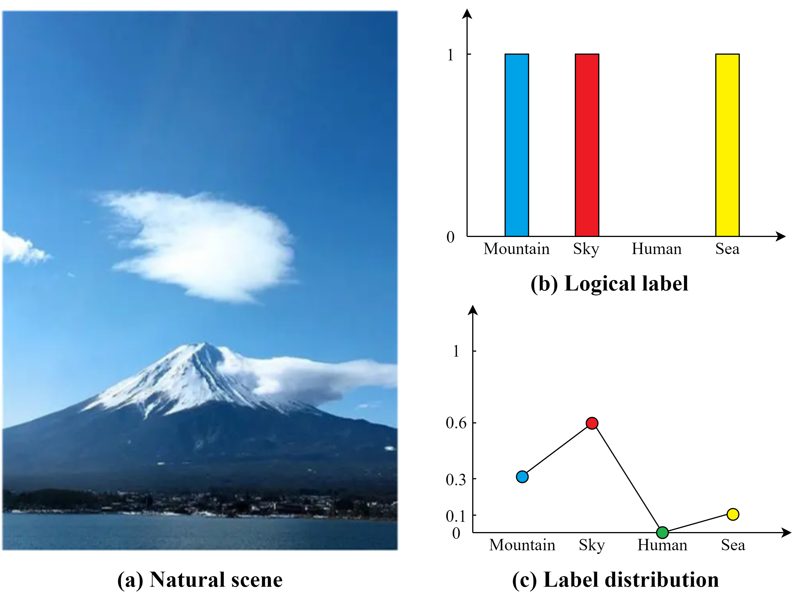
Figure 1: An example of using label distribution to describe a natural scene image in (a). The histogram in (b) denotes the logical label, indicating whether a label can describe the image in (a), and the line chart in (c) shows the label distribution, revealing to what degree a label can describe the image in (a).

In LDL, a training set with samples annotated by LDs is required to train an LDL model. Unfortunately, the acquisition of label distributions of instances is a very costly and time-consuming process. Moreover, in reality, most datasets are only annotated by logical labels, which cannot be used directly by the existing LDL methods. Then a question naturally arises: can we directly train an LDL model from the logical labels?

Recently, label enhancement (LE) Xu et al. (2021) was proposed to partially answer this question. Specifically, LE first recovers the label distributions of training samples from the logical labels and then performs an existing LDL algorithm on the recovered LDs. Following Xu et al. (2021), many variants of LE were proposed, such as Shao et al. (2018), Zheng et al. (2023) and Zhang et al. (2021). We refer the readers to the related work for more details. To achieve LE, those methods generally construct a linear mapping from the features to the logical labels directly, and then normalize the output of the linear mapping as the recovered LDs. However, those LE methods may assign positive description degrees to some negative logical labels. Moreover, as all the positive logical labels are annotated as $1$, simply building a mapping from features to the logical labels is unreasonable, which will not differentiate the description degrees to different labels. Last but not least, the LE-based strategy is a step-wise manner to predict LD for unseen samples, which may lose the connection between LE and LDL model training.

In this paper, we come up with a novel model named DLDL, i.e., Directly Label Distribution Learning from the logical label, which gives a favorable answer to the question “can we directly train an LDL model from the logical labels”. The major contributions of our method are summarized as follows:

• Our model is the first attempt to combine LE and LDL into a single model, which can learn an LDL model directly from the instances annotated by the logical labels. By the joint manner, the LE and LDL processes will better match each other.

• We strictly constrain the description degree $d^{l}_{\boldsymbol{x}}$ to be 0 when the logical value corresponding to the label $l$ is 0. The constraint will avoid assigning positive description degrees to the negative logical labels.

• The existing LE methods usually minimize a least squares loss between the recovered LD and the logical label, which can not differentiate the description degrees of different labels. The proposed model avoids this fidelity term, and uses KL-divergence to minimize the difference between the recovered LD and the predictive LD, which is a better difference measure for two distributions.

Extensive experiments on six benchmark datasets clearly show that the LD recovered by our method is better than that recovered by state-of-the-art LE methods on the training set, and the prediction performance of our model on the testing set also achieves state-of-the-art results compared to the traditional step-wise strategy.

The structure of the paper is as follows. Firstly, we briefly review the related works on LDL and LE in Section 2. Secondly, we present the technical details of our model in Section 3. Then, the experimental results and analyses are presented to prove the effectiveness of our model in Section 4. Finally, conclusions and future working directions are drawn in Section 5.

2 Related Works

Notations: Let $n$, $m$ and $c$ represent the number of samples, the dimension of features, and the number of labels. Let $\boldsymbol{x}\in\mathbb{R}^{m}$ denote a feature vector and $\boldsymbol{y}\in\left\{0,1\right\}^{c}$ denote its corresponding logical label vector. The feature matrix and the corresponding logical label matrix can be denoted by $\mathbf{X}=\left[\boldsymbol{x}_{1};\boldsymbol{x}_{2};\ldots;\boldsymbol{x}_{n}\right]\in\mathbb{R}^{n\times m}$ and $\mathbf{Y}=\left[\boldsymbol{y}_{1};\boldsymbol{y}_{2};\ldots;\boldsymbol{y}_{n}\right]\in\left\{0,1\right\}^{n\times c}$, respectively. Let $\mathcal{Y}=\left\{l_{1},l_{2},\ldots,l_{c}\right\}$ be the complete set of labels. The description degree of the label $l$ to the instance $\boldsymbol{x}$ is denoted by $d^{l}_{\boldsymbol{x}}$, which satisfies $d^{l}_{\boldsymbol{x}}\in\left[0,1\right]$ and $\sum_{l}d^{l}_{\boldsymbol{x}}=1$, and the label distribution of $\boldsymbol{x}_{i}$ is denoted by $\boldsymbol{d}_{i}=\left(d^{l_{1}}_{\boldsymbol{x}_{i}},d^{l_{2}}_{\boldsymbol{x}_{i}},\ldots,d^{l_{c}}_{\boldsymbol{x}_{i}}\right)$.

2.1 Label Distribution Learning

LDL is a new machine learning paradigm that constructs a model to predict the label distribution of samples. At first, LDL were achieved through problem transformation that transforms LDL into a set of single label learning problems such as PT-SVM, PT-Bayes Geng (2016), or through algorithm adaptation that adopts the existing machine learning algorithms to LDL, such as AA-kNN and AA-BP Geng (2016). SA-IIS Geng (2016) is the first model that specially designed for LDL, whose objective function is a mixture of maximum entropy loss Berger et al. (1996) and KL-divergence. Based on SA-IIS, SA-BFGS Geng (2016) adopts BFGS to optimize the loss function, which is faster than SA-IIS. Sparsity conditional energy label distribution learning (SCE-LDL) Yang et al. (2016) is a three-layer energy-based model for LDL. In addition, SCE-LDL is improved by incorporating sparsity constraints into the objective function. To reduce feature noise, latent semantics encoding for LDL (LSE-LDL) Xu et al. (2019) converts the original data features into latent semantic features, and removes some irrelevant features by feature selection. LDL forests (LDLFs) Shen et al. (2017) is based on differentiable decision trees and may be combined with representation learning to provide an end-to-end learning framework. LDL by optimum transport (LDLOT) Zhao and Zhou (2018) builds an objective function using the optimal transport distance measurement and label correlations.

2.2 Label Enhancement

The above mentioned LDL methods all assume that in the training set, each sample is annotated with label distribution. However, precisely annotating the label distributions for the training samples is extremely costly and time-consuming. On the contrary, many datasets annotated by logical labels are readily available. To this end, LE was proposed, which aims to convert the logical labels of samples in training set to label distributions. GLLE Xu et al. (2021) is the first LE algorithm, which assumes that the LDs of two instances are similar to each other if they are similar in the feature space. LEMLL Shao et al. (2018) adopts the local linear embedding technique to evaluate the relationship of samples in the feature spaces. Generalized label enhancement with sample correlations (gLESC) Zheng et al. (2023) tries to obtain the sample correlations from both of the feature and the label spaces. Bidirectional label enhancement (BD-LE) Liu et al. (2021) takes the reconstruction errors from the label distribution space to the feature space into consideration.

All of these LE methods can be generally formulated as

$$\min_{\mathbf{W}}||\mathbf{XW}-\mathbf{Y}||_{F}^{2}+\phi(\mathbf{XW},\mathbf{X}),$$ (1)

where $\mathbf{X}$ and $\mathbf{Y}$ are the feature matrix and logical label matrix, $\|\cdot\|_{F}$ denotes the Frobenius of a matrix, $\mathbf{W}\in\mathbb{R}^{m\times c}$ builds a linear mapping from features to logical labels, and $\phi(\mathbf{XW},\mathbf{X})$ models the geometric structure of samples, which is used to assist LD recovery. After minimizing Eq. (1), those methods usually normalize $\mathbf{XW}$ as the recovered LD.

Although those LE methods have achieved great success, they still suffer from the following limitations. Firstly, the fidelity term that minimizes the distance between the recovered LD $\mathbf{XW}$ and the logical label $\mathbf{Y}$ is inappropriate, because the logical labels are annotated as the same value and the linear mapping will not differentiate the description degrees for different labels. Besides, the Frobenius norm is also not the best choice to measure the difference between two distributions. Secondly, Eq. (1) doesn’t consider the restriction of the label distribution, i.e. $\forall i,\textbf{0}\leq\boldsymbol{d}_{i}\leq\boldsymbol{y}_{i},\sum_{l}d^{l}_{\boldsymbol{x}_{i}}=1$. Although those LE methods performs a post-normalization to satisfy those constraints, they may assign positive description degrees to some negative logical labels. Furthermore, to predict the LD for unseen samples, those methods need to first perform LE and then carry out an existing LDL algorithm. The step-wise manner does not consider potential connections between LE and LDL.

3 The Proposed Approach

To solve the above mentioned issues, we propose a novel model named DLDL. Different from the previous two-step strategy, our method can directly generate a label distribution matrix $\mathbf{D}=\left[\boldsymbol{d}_{1};\boldsymbol{d}_{2};\ldots;\boldsymbol{d}_{n}\right]\in\mathbb{R}^{n\times c}$ for samples annotated by logical labels and at the same time construct a weight matrix $\mathbf{W}\in\mathbb{R}^{m\times c}$ to predict LD for unseen samples.

We use the following priors to recover the LD matrix $\mathbf{D}$ from the logical $\mathbf{Y}$. First, as each row of $\mathbf{D}$ (e.g., $\boldsymbol{d}_{i}$) denotes the recovered LD for a sample, it should obey the non-negative constraint and the sum-to-one constraint to make it a well-defined distribution, i.e., $\mathbf{0}_{c}\leq\boldsymbol{d}_{i}\leq\mathbf{1}_{c}$ and $\boldsymbol{d}_{i}\mathbf{1}_{c}=1$, where $\mathbf{0}_{c}$, $\mathbf{1}_{c}\in\mathbb{R}^{c}$ denote an all-zeros vector and an all-ones vector, and $\mathbf{0}\leq\boldsymbol{d}_{i}\leq\mathbf{1}$ means each element of $\boldsymbol{d}_{i}$ is non-negative and no more than $1$. Moreover, to avoid assigning a positive description to a negative logical label, we require that $\mathbf{0}\leq\boldsymbol{d}_{i}\leq\boldsymbol{y}_{i},\forall i$. Reformulating the above constraints in the matrix form, we have $\mathbf{0}_{m\times c}\leq\mathbf{D}\leq\mathbf{Y},$ $\mathbf{D}\mathbf{1}_{c}=\mathbf{1}_{n}$, where $\mathbf{0}_{m\times c}$ is an all-zeros matrix with size $m\times c$, and the above inequalities are held element-wisely.

Second, we utilize the geometric structure of the samples to help recover the LDs from the logical labels, i.e., if two samples are similar to each other in the feature space, they are likely to own the similar LDs. To capture the similarity among samples, we define the local similarity matrix $\mathbf{A}=\left[A_{ij}\right]_{n\times n}$ as

$$A_{ij}=\begin{aligned} \begin{cases}\exp\left(-\left\|\boldsymbol{x}_{i}-\boldsymbol{x}_{j}\right\|_{2}^{2}/2\sigma^{2}\right),&\text{if }\boldsymbol{x}_{j}\in\mathcal{N}\left(\boldsymbol{x}_{i}\right)\\ 0,\quad&\text{otherwise}.\end{cases}\end{aligned}$$ (2)

$\mathcal{N}\left(\boldsymbol{x}_{i}\right)$ denotes the $k$-nearest neighbors of $\boldsymbol{x}_{i}$, and $\sigma^{2}>0$ is a hyper-parameter. Based on the constructed local similarity matrix $\mathbf{A}$, we can infer that the value of $||\boldsymbol{d}_{i}-\boldsymbol{d}_{j}||$ is small when $A_{ij}$ is large, i.e.,

$$\min_{\mathbf{D}}\ \underset{i,j}{\sum}A_{ij}||\boldsymbol{d}_{i}-\boldsymbol{d}_{j}||_{2}^{2}=\rm{tr}\left(\mathbf{D}^{T}\mathbf{G}\mathbf{D}\right),$$ (3)

in which $\rm{tr}\left(\cdot\right)$ denotes the trace of a matrix, and $\mathbf{G}=\hat{\mathbf{A}}-\mathbf{A}$ is the graph Laplacian matrix and $\hat{\mathbf{A}}$ is a diagonal matrix with the elements $\hat{A}_{ii}=\sum_{j=1}^{n}A_{ij}$.

By taking the above priors into consideration, the LD matrix $\mathbf{D}$ can be inferred from the logical label matrix $\mathbf{Y}$, i.e.,

$$\underset{\mathbf{D}}{\min}\ \rm{tr}\left(\mathbf{D}\mathbf{G}\mathbf{D}^{T}\right)+||\mathbf{D}||_{F}^{2}$$ (4)

$$\text{s.t.}\ \textbf{0}_{m\times c}\leq\mathbf{D}\leq\mathbf{Y},\mathbf{D}\mathbf{1}_{c}=\mathbf{1}_{n},$$

where an additional term $\|\mathbf{D}\|_{F}^{2}$ is imposed as regularization.

Based on the recovered LD, we adopt a non-linear model that maps the features to the recovered LD, which can be used to predict the LD for unseen samples. Specifically, the non-linear model is formulated as

$$P_{ij}=\dfrac{1}{Z}\exp\left(\sum^{m}_{k=1}X_{ik}W_{kj}\right),$$ (5)

where $\mathbf{W}$ is the weight matrix, $\mathbf{P}=[P_{ij}]_{n\times n}$ is the prediction matrix, and $Z=\sum^{c}_{j=1}\exp\left(\sum^{m}_{k=1}X_{ik}W_{kj}\right)$ is a normalization term. To infer the weight matrix $\mathbf{W}$, we minimize the KL-divergence between the recovered label distribution matrix $\mathbf{D}$ and the prediction matrix $\mathbf{P}$, because KL-divergence is a good metric to measure the difference between the two distributions. Accordingly, the loss function for inferring $\mathbf{W}$ becomes

$$\underset{\mathbf{W}}{\min}\ \rm{KL}(\mathbf{D},\mathbf{P})+||\mathbf{W}||_{F}^{2},$$ (6)

where the widely-used squared Frobenius norm is imposed to control the model complexity.

To directly induce an LD prediction model from the logical labels, we combine Eqs. (4) and (6) together and the final optimization problem of our method becomes:

$$\underset{\mathbf{D},\mathbf{W}}{\min}\ \rm{KL}(\mathbf{D},\mathbf{P})+\alpha tr\left(\mathbf{D}\mathbf{G}\mathbf{D}^{T}\right)+\beta||\mathbf{D}||_{F}^{2}+\gamma||\mathbf{W}||_{F}^{2}$$ (7)

$$\text{s.t.}\ \textbf{0}_{m\times c}\leq\mathbf{D}\leq\mathbf{Y},\mathbf{D}\mathbf{1}_{c}=\mathbf{1}_{n},$$

in which $\alpha$, $\beta$ and $\gamma$ are hyper-parameters to adjust the contributions of different terms. By minimizing Eq. (7), the proposed model can recover the LD for samples with logical labels, and simultaneously, can predict LD for unseen samples through Eq. (5).

3.1 Optimization

Eq. (7) has two variables, we solve it by an alternative iterative process, i.e., update $\mathbf{W}$ with fixed $\mathbf{D}$, and then update $\mathbf{D}$ with fixed $\mathbf{W}$.

3.1.1 Update W

When $\mathbf{D}$ is fixed, the optimization problem (7) with respect to $\mathbf{W}$ can be formulated as follows:

$$\underset{\mathbf{W}}{\min} \rm{KL}(\mathbf{D},\mathbf{P})+\gamma||\mathbf{W}||_{F}^{2}.$$ (8)

Expanding the KL-divergence and substituting $P_{ij}$ in Eq. (5) into Eq. (8), we obtain the objective function of $\mathbf{W}$ as

$$T(\mathbf{W})= \sum_{i}{\rm ln}\sum_{j}\exp\left(\sum_{k}X_{ik}W_{kj}\right)+\gamma||\mathbf{W}||_{F}^{2}$$ (9)

$$-\sum_{i,j}D_{ij}\sum_{k}X_{ik}W_{kj}.$$

Eq. (9) is a convex problem, we use gradient descent algorithm to update $\mathbf{W}$, where the gradient is expressed as

$$\dfrac{\partial\ T\left(\mathbf{W}\right)}{\partial\ W_{kj}}= \sum_{i}\dfrac{\exp\left(\sum_{k}X_{ik}W_{kj}\right)X_{ik}}{\sum_{j}\exp\left(\sum_{k}X_{ik}W_{kj}\right)}$$ (10)

$$-\sum_{i}D_{ij}X_{ik}+2\gamma W_{kj}.$$

Algorithm 1 Solve the Problem in (11)

Input: The initial $\mathbf{D}$, $\mathbf{W}$, and $\mathbf{B}=\mathbf{\Phi}=\mathbf{0}_{n\times c}$.
Parameter: $\rho=1.1$, $\tau=1$ and $\tau_{max}=10^{3}$.
Output: $\mathbf{D}$.

1:  while $||\mathbf{B}-\mathbf{D}||_{\infty}>10^{-3}$ do

2:     Update $\mathbf{D}$ by Eq. (14);

3:     Update $\mathbf{B}$ by solving Eq. (16);

4:     Update $\mathbf{\Phi}=\mathbf{\Phi}+\tau(\mathbf{B}-\mathbf{D})$ and $\tau=\min(\rho\tau,\tau_{max})$;

5:  end while

Algorithm 2 The DLDL Algorithm

Input: The feature matrix $\mathbf{X}$ and the logical label matrix $\mathbf{Y}$.
Parameter: $\alpha,\beta,\lambda$ and $\sigma$.
Output: The label distribution matrix $\mathbf{D}$ and the weight matrix $\mathbf{W}$.

1:  Initialize $\mathbf{W}$ and $\mathbf{D}$.

2:  Specify the maximum of iterations $t$.

3:  repeat

4:     Update $\mathbf{W}$ by using Eq. (10);

5:     Update $\mathbf{D}$ by Algorithm 2;

6:  until convergence or reaches the maxiter $t$;

7:  return $\mathbf{D}$ and $\mathbf{W}$.

3.1.2 Update D

With fixed $\mathbf{W}$, the optimization problem (7) regarding $\mathbf{D}$ is formulated as

$$\underset{\mathbf{D}}{\min}\ \rm{KL}(\mathbf{D},\mathbf{P})+\alpha\rm{tr}\left(\mathbf{D}\mathbf{G}\mathbf{D}^{T}\right)+\beta||\mathbf{D}||_{F}^{2}$$ (11)

$$\text{s.t.}\ \textbf{0}\leq\mathbf{D}\leq\mathbf{Y},\mathbf{D}\mathbf{1}_{c}=\mathbf{1}_{n}.$$

Eq. (11) involves multiple constraints and diverse losses, we introduce an auxiliary variable $\mathbf{B}=\mathbf{D}\in\mathbb{R}^{n\times c}$ to simplify it, and the corresponding augmented Lagrange equation becomes

$$\underset{\mathbf{D},\mathbf{B}}{\min}\ \rm{KL}(\mathbf{D},\mathbf{P})+\alpha\rm{tr}\left(\mathbf{D}^{T}\mathbf{G}\mathbf{D}\right)+\beta||\mathbf{D}||_{F}^{2}$$ (12)

$$\qquad\qquad+\left<\mathbf{\Phi},\mathbf{B}-\mathbf{D}\right>+\frac{\tau}{2}||\mathbf{B}-\mathbf{D}||^{2}_{F}$$

$$\text{s.t.}\ \textbf{0}\leq\mathbf{B}\leq\mathbf{Y},\mathbf{B}\mathbf{1}_{c}=\mathbf{1}_{n},$$

where $\mathbf{\Phi}\in\mathbb{R}^{n\times c}$ is the Lagrange multiplier, and $\tau$ is parameter to introduce the augmented equality constraint. Eq. (12) can be minimized by solving the following sub-problems iteratively.

1) $\mathbf{D}$-subproblem: Removing the irrelated terms regarding $\mathbf{D}$, the $\mathbf{D}$-subproblem of Eq. (12) becomes

$$\underset{\mathbf{D}}{\min}\ \rm{KL}(\mathbf{D},\mathbf{P})+\alpha\rm{tr}\left(\mathbf{D}^{T}\mathbf{G}\mathbf{D}\right)+\beta||\mathbf{D}||_{F}^{2}$$ (13)

$$\qquad\qquad+\left<\mathbf{\Phi},\mathbf{B}-\mathbf{D}\right>+\frac{\tau}{2}||\mathbf{B}-\mathbf{D}||^{2}_{F}.$$

Eq. (LABEL:Dsubproblem) is solved when its gradient regarding $\mathbf{D}$ vanishes, leading to

$$\mathbf{D}=(\mathbf{X}\mathbf{W}+\mathbf{\Phi}+\tau\mathbf{B})(2\beta+\alpha(\mathbf{G}+\mathbf{G}^{T})+\tau)^{-1}.$$ (14)

2) $\mathbf{B}$-subproblem: When $\mathbf{D}$ is fixed, the problem (12) can be written as

$$\underset{\mathbf{B}}{\min}\ \left<\mathbf{\Phi},\mathbf{B}-\mathbf{D}\right>+\frac{\tau}{2}||\mathbf{B}-\mathbf{D}||^{2}_{F}$$ (15)

$$\text{s.t.}\ \textbf{0}\leq\mathbf{B}\leq\mathbf{Y},\mathbf{B}\mathbf{1}_{c}=\mathbf{1}_{n}.$$

Let $\hat{\boldsymbol{b}}=[\boldsymbol{b}_{1}^{T};\boldsymbol{b}_{2}^{T};\cdots;\boldsymbol{b}_{n}^{T}]\in\mathbb{R}^{nc}=vec(\mathbf{B})$, where $\boldsymbol{b}_{i}$ is the $i$-th row of $\mathbf{B}$ and $vec(\cdot)$ is the vectorization operator. Then, the problem (15) is equivalent to:

$$\underset{\hat{\boldsymbol{b}}}{\min}\ \hat{\boldsymbol{b}}^{T}\mathbf{\Sigma}\hat{\boldsymbol{b}}-\left(2\hat{\boldsymbol{d}}^{T}+\frac{2}{\tau}\hat{\boldsymbol{\phi}}^{T}\right)\hat{\boldsymbol{b}}$$ (16)

$$\text{s.t.}\ \mathbf{0}_{nc}\leq\hat{\boldsymbol{b}}\leq\hat{\boldsymbol{y}},\sum_{j=c(i-1)+1}^{ci}\hat{\boldsymbol{b}}_{j}=1\ \left(\forall\ 0\leq i\leq n\right),$$

in which $\hat{\boldsymbol{d}}$, $\hat{\boldsymbol{\phi}}$ and $\hat{\boldsymbol{y}}$ represent $vec(\mathbf{D})$, $vec(\mathbf{\Phi})$ and $vec(\mathbf{Y})$, respectively, and $\hat{\boldsymbol{b}}_{j}$ is the $j$-th element of $\hat{\boldsymbol{b}}$. Eq. (16) is a quadratic programming (QP) problem that can be solved by off-the-shelf QP tools.

The detailed solution to update $\mathbf{D}$ in Eq. (11) is summarized in Algorithm 1.

3.1.3 Initialization of W and D

The above alternative updating of $\mathbf{W}$ and $\mathbf{D}$ needs an initialization of them. As is suggested by Wang et al. (2023), we initialize $\mathbf{W}$ as an identity matrix and we initialize $\mathbf{D}$ by the pseudo label distribution matrix in Wang et al. (2023).

The pseudo code of DLDL is finally presented in Algorithm 2.

Table 1: Statistics of the evaluated datasets.

Dataset (abbr.)	# Instances	# Features	# Labels
Natural Scene (NS)	1200	294	9
SCUT_FBP (SCUT)	1500	300	5
RAF_ML (RAF)	4908	200	6
SCUT-FBP5500 (FBP)	5500	512	5
Ren-Cecps (REN)	3000	100	8
Twitter_LDL (Twitter)	6027	200	8

4 Experiments

4.1 Real-World Datasets

We select six real-world datasets from various fields for experiment, and samples in each dataset are annotated by LDs. The statistics of the six datasets are shown in Table 1. Natural Scene Geng (2016); Geng et al. (2022) is generated from the preference distribution of each scene image, SCUT-FBP Xie et al. (2015) is a benchmark dataset for facial beauty perception, RAF-ML Shang and Deng (2019) is a multi-label facial expression dataset, SCUT-FBP5500 Liang et al. (2018) is a big dataset for facial beauty prediction, Ren_CECps Quan and Ren (2009) is a Chinese emotion corpus of weblog articles, and Twitter_LDL Yang et al. (2017) is a visual sentiment dataset.

To verify whether our method can directly learn an LDL model from the logical labels, we generate the logical labels from the ground-truth LDs. Specifically, when the description degree is higher than a predefined threshold $\delta$, we set the corresponding logical label to 1; otherwise, the corresponding logical label is 0. In this paper, $\delta$ is fixed to 0.01.

4.2 Baselines and Settings

In this paper, we split each dataset into three subsets: training set (60%), validation set (20%) and testing set (20%). The training set is used for recovery experiments, that is, we perform LE methods to recover the LDs of training instances; the validation set is used to select the optimal hyper-parameters for each LE algorithms; the testing set is used for predictive experiments, that is, we use an LDL model learned from the training set with the recovered LDs to predict the LDs of testing instances.

In the recovery experiment, for our method DLDL, $\alpha$ and $\gamma$ are chosen among {$10^{-3},10^{-2},\cdots,10,10^{2}$}, $\beta$ is selected from {$10^{-3},10^{-2},\cdots,1,10$}, and the maximum of iterations t is fixed to 10. We compare DLDL with five state-of-the-art LE methods, each configured with suggested configurations in respective literature:

• FLE Wang et al. (2023): $\alpha$, $\beta$, $\lambda$, $\gamma$ are chosen among {$10^{-3},10^{-2},\cdots,10,10^{2}$}.

• GLLE Xu et al. (2021): $\lambda$ is chosen among {$10^{-3},10^{-2},\cdots,1$}.

• LEMLL Shao et al. (2018): the number of neighbors $K$ is set to 10 and $\epsilon$ is set to 0.2.

• LESC Zheng et al. (2023): $\beta$ is set to 0.001 and $\gamma$ is set to 1.

• FCM Gayar et al. (2006): the number of clustering centers is set to 10 times of the number of labels.

In the predictive experiment, we apply BFGS-LLD Geng (2016) algorithm to predict the LDs of testing instances based on the recovered LDs by performing the five baseline LE methods. Note that our model can directly predict the LDs without an external LDL model.

As suggested in Geng (2016), we adopt three distance metrics (i.e., Chebyshev, Clark and Canberra) and one similarity metric (i.e., Intersection) to evaluate the recovery performance and the predictive performance.

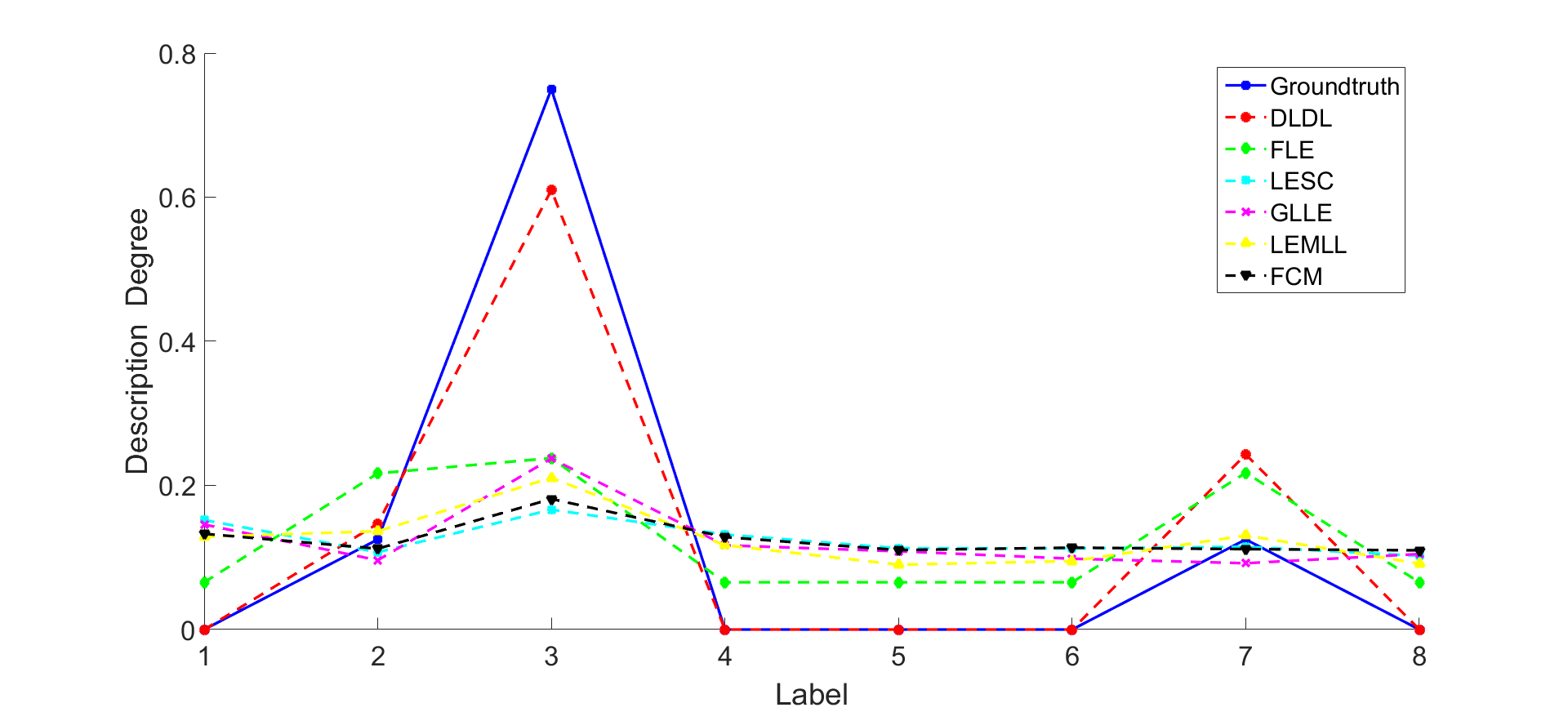
Figure 2: The visualization of one typical recovery results on the Twitter dataset.

4.3 Results

Table 2: The recovery results on six datasets and the best average rank is shown in boldface.

Method	Chebyshev$\downarrow$						Avgrank
	NS	SCUT	RAF	FBP	REN	Twitter
DLDL	0.0869(1)	0.2456(1)	0.3157(1)	0.2610(1)	0.0374(1)	0.1916(1)	1.00(1)
FLE	0.0982(2)	0.3600(6)	0.3844(5)	0.3635(4)	0.5865(3)	0.2111(2)	3.67(4)
GLLE	0.3368(5)	0.3327(2)	0.3453(3)	0.3479(2)	0.6663(5)	0.4676(4)	3.50(2)
LEMLL	0.3151(3)	0.3366(3)	0.3586(4)	0.3556(3)	0.6253(4)	0.4639(3)	3.33(2)
LESC	0.3358(4)	0.3508(5)	0.3408(2)	0.3676(5)	0.6728(6)	0.5022(5)	4.50(5)
FCM	0.3570(6)	0.3464(4)	0.3888(6)	0.3698(6)	0.3905(2)	0.5053(6)	5.00(6)
Method	Clark$\downarrow$						Avgrank
	NS	SCUT	RAF	FBP	REN	Twitter
DLDL	2.1169(1)	1.4535(2)	1.0379(1)	1.5037(6)	2.5515(1)	2.3505(2)	2.17(1)
FLE	2.2836(2)	1.4693(6)	1.6517(6)	1.4845(3)	2.6351(2)	2.3363(1)	3.33(3)
GLLE	2.4440(4)	1.4440(1)	1.5770(3)	1.4697(1)	2.6603(5)	2.3641(4)	3.00(2)
LEMLL	2.4205(3)	1.4592(5)	1.6112(4)	1.4889(5)	2.6385(3)	2.3572(3)	3.83(4)
LESC	2.4480(5)	1.4580(4)	1.5736(2)	1.4867(4)	2.6639(6)	2.3782(5)	4.33(5)
FCM	2.4644(6)	1.4545(3)	1.6294(5)	1.4834(2)	2.6478(4)	2.3818(6)	4.33(5)
Method	Canberra$\downarrow$						Avgrank
	NS	SCUT	RAF	FBP	REN	Twitter
DLDL	5.2948(1)	2.7084(1)	1.8966(1)	2.8234(1)	6.5966(2)	5.9575(2)	1.33(1)
FLE	5.8290(2)	2.8742(6)	3.5965(6)	2.8814(3)	7.2428(3)	5.9355(1)	3.50(2)
GLLE	6.7293(4)	2.7873(2)	3.3695(3)	2.8414(2)	7.4155(5)	6.0873(4)	3.33(2)
LEMLL	6.5789(3)	2.8289(3)	3.4761(4)	2.8907(4)	7.2982(4)	6.0620(3)	3.50(4)
LESC	6.7705(5)	2.8386(5)	3.3561(2)	2.8973(6)	7.4310(6)	6.1473(6)	5.00(6)
FCM	6.8686(6)	2.8255(4)	3.5599(5)	2.8923(5)	3.6063(1)	6.1465(5)	4.33(5)
Method	Intersection$\uparrow$						Avgrank
	NS	SCUT	RAF	FBP	REN	Twitter
DLDL	0.8999(1)	0.7218(1)	0.6262(1)	0.7150(1)	0.9624(1)	0.7986(1)	1.00(1)
FLE	0.8765(2)	0.5339(6)	0.5216(5)	0.6172(2)	0.3271(3)	0.7850(2)	3.33(2)
GLLE	0.4484(4)	0.5816(2)	0.5674(3)	0.5881(3)	0.2128(5)	0.4341(4)	3.50(3)
LEMLL	0.4933(3)	0.5766(3)	0.5536(4)	0.5772(4)	0.2705(4)	0.4582(3)	3.50(3)
LESC	0.4354(5)	0.5500(5)	0.5744(2)	0.5621(5)	0.2044(6)	0.3959(5)	4.67(5)
FCM	0.3980(6)	0.5578(4)	0.4962(6)	0.5387(6)	0.4916(2)	0.3831(6)	5.00(6)

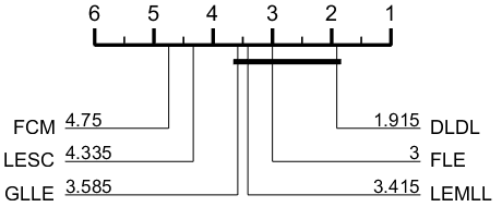
(a) Chebyshev

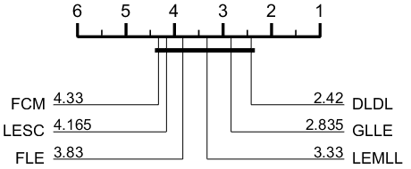
(b) Clark

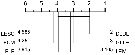
(c) Canberra

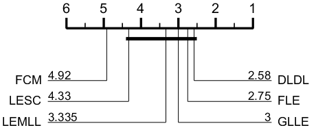
(d) Intersection

Figure 3: Comparison of DLDL against other five methods with the Bonferroni-Dunn test (CD = 2.1765 at 0.05 significance level).

4.3.1 Recovery Results

In this subsection, we calculate the distances and similarities between the ground-truth LD and the LD recovered by each LE method via four evaluation metrics on each dataset. Table 2 shows the detailed recovery results, where all methods are ranked according to their performance and the best average rank on each metric is shown in boldface. In addition, the “$\downarrow$” after the metrics means “the smaller the greater”, while the “$\uparrow$” means “the larger the greater”. Based on the recovery results, we have the following observations:

• DLDL achieves the lowest average rank in terms of all the four evaluation metrics. To be specific, out of the 24 statistical comparisons (6 datasets × 4 evaluation metrics), DLDL ranks 1st in 79.2% cases and ranks 2nd in 16.7% cases, which clearly shows the superiority of our approach in LE.

• On some datasets, our method achieves superior performance. For example, on SCUT, REN and FBP, DLDL significantly improves the results compared with other algorithms in terms of the Chebyshev and Intersection.

• Although the average ranks of FLE and GLLE are low, they do not perform well on all datasets as DLDL does. Specifically, FLE performs poorly on SCUT and RAF, and GLLE performs poorly on NS, REN and Twitter. From this point of view, DLDL is more robust to different datasets than comparison algorithms.

Moreover, Fig. 2 shows the recovery results of a typical sample on the Twitter dataset. For this sample, the logical values corresponding to the label 1, 4, 5, 6, 8 are all 0, indicating that these labels cannot describe this sample. However, the five comparison methods still assign positive description degrees for these invalid labels. Differently, DLDL avoids this problem, and produces differentiated description degrees fairly close to the ground-truth values.

Table 3: The predictive results of testing instances on the six datasets and the best average rank is shown in boldface.

Method	Chebyshev$\downarrow$						Avgrank
	NS	SCUT	RAF	FBP	REN	Twitter
BFGS-LLD	0.3533	0.4202	0.1583	0.3323	0.5871	0.3532	-
DLDL	0.3841(6)	0.4074(1)	0.3009(1)	0.4543(6)	0.6543(2)	0.2610(1)	2.83(2)
FLE	0.3436(1)	0.4189(2)	0.3622(5)	0.3471(1)	0.6558(3)	0.3485(2)	2.33(1)
GLLE	0.3626(4)	0.4207(5)	0.3446(3)	0.3734(2)	0.6573(5)	0.4692(3)	3.67(4)
LEMLL	0.3596(2)	0.4202(3)	0.3548(4)	0.3781(4)	0.6566(4)	0.4728(4)	3.50(3)
LESC	0.3605(3)	0.4204(4)	0.3393(2)	0.3969(5)	0.6629(6)	0.4975(5)	4.17(5)
FCM	0.3758(5)	0.4223(6)	0.3893(6)	0.3764(3)	0.3975(1)	0.5082(6)	4.50(6)
Method	Clark$\downarrow$						Avgrank
	NS	SCUT	RAF	FBP	REN	Twitter
BFGS-LLD	2.4212	1.5491	1.4531	1.4703	2.6407	2.5577	-
DLDL	2.4205(1)	1.5346(1)	1.5174(1)	1.5486(6)	1.5696(1)	2.4302(6)	2.67(1)
FLE	2.4893(6)	1.5428(5)	1.6015(5)	1.4798(1)	2.6562(4)	2.3868(5)	4.33(5)
GLLE	2.4756(3)	1.5424(2)	1.5689(3)	1.4850(2)	2.6567(5)	2.3678(1)	2.67(1)
LEMLL	2.4742(2)	1.5424(2)	1.5808(4)	1.4886(4)	2.6560(3)	2.3680(2)	2.83(3)
LESC	2.4771(4)	1.5426(4)	1.5628(2)	1.5022(5)	2.6597(6)	2.3813(3)	4.00(4)
FCM	2.4864(5)	1.5437(6)	1.6274(6)	1.4883(3)	1.6440(2)	2.3850(4)	4.33(5)
Method	Canberra$\downarrow$						Avgrank
	NS	SCUT	RAF	FBP	REN	Twitter
BFGS-LLD	6.6811	3.0817	2.8239	2.8963	7.2720	6.9345	-
DLDL	6.7268(1)	3.0397(1)	3.1553(1)	3.0804(6)	3.1489(1)	6.3263(6)	2.67(1)
FLE	6.9338(5)	3.0682(5)	3.6564(6)	2.8388(1)	7.4012(4)	6.2145(5)	4.33(6)
GLLE	6.8828(3)	3.0663(2)	3.3583(3)	2.8995(2)	7.4036(5)	6.1032(1)	2.67(1)
LEMLL	6.8771(2)	3.0663(2)	3.4012(4)	2.9109(4)	7.4007(3)	6.1061(2)	2.83(3)
LESC	6.9119(4)	3.0666(4)	3.3363(2)	2.9536(5)	7.4169(6)	6.1728(4)	4.17(4)
FCM	6.9613(6)	3.0717(6)	3.5701(5)	2.9099(3)	3.6082(2)	6.1574(3)	4.17(4)
Method	Intersection$\uparrow$						Avgrank
	NS	SCUT	RAF	FBP	REN	Twitter
BFGS-LLD	0.5183	0.4731	0.8029	0.6226	0.3269	0.6035	-
DLDL	0.4980(1)	0.4902(1)	0.6340(1)	0.4779(6)	0.3421(2)	0.6811(1)	2.00(1)
FLE	0.4602(2)	0.4711(2)	0.5398(5)	0.5867(1)	0.2145(3)	0.5580(2)	2.50(2)
GLLE	0.4181(4)	0.4707(3)	0.5647(3)	0.5414(2)	0.2128(5)	0.4312(3)	3.33(3)
LEMLL	0.4207(3)	0.4705(4)	0.5502(4)	0.5357(4)	0.2139(4)	0.4287(4)	3.83(4)
LESC	0.4085(5)	0.4705(4)	0.5725(2)	0.5123(5)	0.2055(6)	0.3953(5)	4.50(5)
FCM	0.3849(6)	0.4680(6)	0.4913(6)	0.5358(3)	0.4853(1)	0.3820(6)	4.67(6)

4.3.2 Predictive Results

In this subsection, BFGS-LLD is used as the predictive model to generate the LDs of testing instances for the five comparison methods, while our model can directly predict the LDs of testing instances. Then, we rank all methods and highlight the best average rank on each metric in boldface. The detailed predictive results are presented in Table 3. In addition, BFGS-LLD is trained on the ground-truth LDs of the training instances and its results are recorded as the upper bound of the prediction results. From the reported results, we observe that:

• DLDL achieves the lowest average rank in terms of the three evaluation metrics (i.e., Clark, Canberra and Intersection). Specifically, out of the 24 statistical comparisons, DLDL ranks 1st in 62.5% cases and ranks 2nd in 8.33% cases. In general, DLDL performs better than most comparison algorithms.

• In some cases, the performance of our approach even exceeds the upper bound. For example, on SCUT dataset, DLDL performs better than the BFGS-LLD trained on the ground-truth LDs in terms of all the four evaluation metrics, which shows that our model has considerable potential in learning from logical labels.

4.4 Further Analysis

Table 4: Ablation study (recovery results)

Method	Chebyshev$\downarrow$
	NS	SCUT	RAF	FBP	REN	Twitter
DLDL	0.0869	0.2456	0.3157	0.2610	0.0374	0.1916
$\alpha=0$	0.1374	0.2889	0.3047	0.3137	0.0692	0.1783
$\beta=0$	0.5861	0.5803	0.6992	0.5131	0.2178	0.4022
$\gamma=0$	0.1189	0.2839	0.3067	0.2613	0.0392	0.1903

Table 5: Ablation study (predictive results)

Method	Chebyshev$\downarrow$
	NS	SCUT	RAF	FBP	REN	Twitter
DLDL	0.3841	0.4074	0.3009	0.4543	0.6543	0.2610
$\alpha=0$	0.5441	0.4198	0.3072	0.4867	0.7337	0.5356
$\beta=0$	0.5751	0.4234	0.4299	0.4877	0.6890	0.7558
$\gamma=0$	0.4868	0.4209	0.3518	0.5014	0.7232	0.5494

4.4.1 Ablation Study

In order to verify the necessity of the involved terms of our approach, we conduct ablation experiments and present the results on Chebyshev in Tables 4 and 5, where $\alpha$, $\beta$ and $\gamma$ are hyper-parameters to adjust the contributions of different terms. When one of hyper-parameters is fixed to 0, the remaining ones are determined by the performance on the validation set.

From the results, we observe that the performance of DLDL becomes poor when the term controlled by $\beta$ is missing, indicating that it is critical to control the smoothness of the label distribution matrix $\mathbf{D}$. In general, DLDL outperforms its variants without some terms, which verify the effectiveness and rationality of our model.

4.4.2 Significance Test

In this subsection, we use the Bonferroni–Dunn test at the 0.05 significance level to test whether DLDL achieves competitive performance compared to other algorithms. Specifically, we combine the recovery results with the predictive results to conduct the Bonferroni-Dunn test, that is, the number of algorithms is 6 and the number of datasets is considered as 12 (2 groups of experiments × 6 datasets). Then, we use DLDL as the control algorithm with a critical difference (CD) to correct for the mean level difference with the comparison algorithms.

The results are shown in Fig. 3, where the algorithms not connected with DLDL are considered to have significantly different performance from the control algorithms. It is impressive that DLDL achieves the lowest rank in terms of all evaluation metrics and is comparable to FLE, GLLE and LEMLL based on all evaluation metrics.

5 Conclusion and Future Work

This paper gives a preliminary positive answer to the question “can we directly train an LDL model from the logical labels”. Specifically, we propose a new algorithm called DLDL, which unifies the conventional label enhancement and label distribution learning into a joint model. Moreover, the proposed method avoids some common issues faced by the previous LE methods. Extensive experiments validate the advantage of DLDL against other LE algorithms in label enhancement, and also confirm the effectiveness of our method in directly training an LDL model from the logical labels. Nevertheless, our method is still inferior to the traditional LDL model when the ground-truth LD of the training set is available. In the future, we will explore possible ways to improve the predictive performance of our algorithm.

References

- Berger et al. [1996] Adam L. Berger, Stephen Della Pietra, and Vincent J. Della Pietra. A maximum entropy approach to natural language processing. Computational Linguistics, 22(1):39–71, 1996.
- Gayar et al. [2006] Neamat El Gayar, Friedhelm Schwenker, and Günther Palm. A study of the robustness of KNN classifiers trained using soft labels. In Artificial Neural Networks in Pattern Recognition, Second IAPR Workshop, pages 67–80. Springer, 2006.
- Geng et al. [2022] Xin Geng, Renyi Zheng, Jiaqi Lv, and Yu Zhang. Multilabel ranking with inconsistent rankers. IEEE Transactions on Pattern Analysis & Machine Intelligence, 44(09):5211–5224, 2022.
- Geng [2016] Xin Geng. Label distribution learning. IEEE Transactions on Knowledge and Data Engineering, 28(7):1734–1748, 2016.
- Liang et al. [2018] Lingyu Liang, Luojun Lin, Lianwen Jin, Duorui Xie, and Mengru Li. SCUT-FBP5500: A diverse benchmark dataset for multi-paradigm facial beauty prediction. In 24th International Conference on Pattern Recognition, pages 1598–1603. IEEE Computer Society, 2018.
- Liu et al. [2021] Xinyuan Liu, Jihua Zhu, Qinghai Zheng, Zhongyu Li, Ruixin Liu, and Jun Wang. Bidirectional loss function for label enhancement and distribution learning. Knowledge-Based Systems, 213:106690, 2021.
- Quan and Ren [2009] Changqin Quan and Fuji Ren. Construction of a blog emotion corpus for chinese emotional expression analysis. In Proceedings of the 2009 conference on empirical methods in natural language processing, pages 1446–1454, 2009.
- Shang and Deng [2019] Li Shang and Weihong Deng. Blended emotion in-the-wild: Multi-label facial expression recognition using crowdsourced annotations and deep locality feature learning. International Journal of Computer Vision, 127(6-7):884–906, 2019.
- Shao et al. [2018] Ruifeng Shao, Ning Xu, and Xin Geng. Multi-label learning with label enhancement. In 2018 IEEE International Conference on Data Mining (ICDM), pages 437–446, 2018.
- Shen et al. [2017] Wei Shen, Kai Zhao, Yilu Guo, and Alan L. Yuille. Label distribution learning forests. CoRR, abs/1702.06086, 2017.
- Tsoumakas and Katakis [2007] Grigorios Tsoumakas and Ioannis Katakis. Multi-label classification: An overview. International Journal of Data Warehousing and Mining, 3(3):1–13, 2007.
- Wang et al. [2023] Ke Wang, Ning Xu, Miaogen Ling, and Xin Geng. Fast label enhancement for label distribution learning. IEEE Transactions on Knowledge and Data Engineering, 35(2):1502–1514, 2023.
- Xie et al. [2015] Duorui Xie, Lingyu Liang, Lianwen Jin, Jie Xu, and Mengru Li. Scut-fbp: A benchmark dataset for facial beauty perception. In 2015 IEEE International Conference on Systems, Man, and Cybernetics, pages 1821–1826, 2015.
- Xu et al. [2019] Suping Xu, Lin Shang, and Furao Shen. Latent semantics encoding for label distribution learning. In Proceedings of the Twenty-Eighth International Joint Conference on Artificial Intelligence, pages 3982–3988. ijcai.org, 2019.
- Xu et al. [2021] Ning Xu, Yun-Peng Liu, and Xin Geng. Label enhancement for label distribution learning. IEEE Transactions on Knowledge and Data Engineering, 33(4):1632–1643, 2021.
- Yang et al. [2016] Xu Yang, Xin Geng, and Deyu Zhou. Sparsity conditional energy label distribution learning for age estimation. In Proceedings of the Twenty-Fifth International Joint Conference on Artificial Intelligence, pages 2259–2265. IJCAI/AAAI Press, 2016.
- Yang et al. [2017] Jufeng Yang, Ming Sun, and Xiaoxiao Sun. Learning visual sentiment distributions via augmented conditional probability neural network. In Proceedings of the Thirty-First AAAI Conference on Artificial Intelligence, pages 224–230. AAAI Press, 2017.
- Zhang and Zhou [2014] Min-Ling Zhang and Zhi-Hua Zhou. A review on multi-label learning algorithms. IEEE Transactions on Knowledge and Data Engineering, 26(8):1819–1837, 2014.
- Zhang et al. [2021] Min-Ling Zhang, Qian-Wen Zhang, Jun-Peng Fang, Yu-Kun Li, and Xin Geng. Leveraging implicit relative labeling-importance information for effective multi-label learning. IEEE Transactions on Knowledge and Data Engineering, 33(5):2057–2070, 2021.
- Zhao and Zhou [2018] Peng Zhao and Zhi-Hua Zhou. Label distribution learning by optimal transport. In Proceedings of the Thirty-Second AAAI Conference on Artificial Intelligence, (AAAI-18), the 30th innovative Applications of Artificial Intelligence (IAAI-18), and the 8th AAAI Symposium on Educational Advances in Artificial Intelligence (EAAI-18), pages 4506–4513. AAAI Press, 2018.
- Zheng et al. [2023] Qinghai Zheng, Jihua Zhu, Haoyu Tang, Xinyuan Liu, Zhongyu Li, and Huimin Lu. Generalized label enhancement with sample correlations. IEEE Transactions on Knowledge and Data Engineering, 35(1):482–495, 2023.