Transformer-based Planning for Symbolic Regression

Abstract

Symbolic regression (SR) is a challenging task in machine learning that involves finding a mathematical expression for a function based on its values. Recent advancements in SR have demonstrated the effectiveness of pre-trained transformer-based models in generating equations as sequences, leveraging large-scale pre-training on synthetic datasets and offering notable advantages in terms of inference time over classical Genetic Programming (GP) methods. However, these models primarily rely on supervised pre-training goals borrowed from text generation and overlook equation discovery objectives like accuracy and complexity. To address this, we propose TPSR, a Transformer-based Planning strategy for Symbolic Regression that incorporates Monte Carlo Tree Search into the transformer decoding process. Unlike conventional decoding strategies, TPSR enables the integration of non-differentiable feedback, such as fitting accuracy and complexity, as external sources of knowledge into the transformer-based equation generation process. Extensive experiments on various datasets show that our approach outperforms state-of-the-art methods, enhancing the model’s fitting-complexity trade-off, extrapolation abilities, and robustness to noise .

1 Introduction

Symbolic regression (SR) is a powerful method to discover mathematical expressions for governing equations of complex systems and to describe data patterns in an interpretable symbolic form. It finds extensive applications in science and engineering, enabling the modeling of physical phenomena in various domains such as molecular dynamics, fluid dynamics, and cosmology [1, 2, 3, 4, 5, 6]. Symbolic representations provide valuable insights into complex systems, facilitating a better understanding, prediction, and control of these systems through the design of accurate, generalizable, and efficient models [7, 8, 9]. SR models establish the functional relationship between independent and target variables by mapping them to mathematical equations. The input data can be obtained from simulations, experimental measurements, or real-world observations. Symbolic regression, however, poses several challenges, including the combinatorial nature of the optimization search space, vulnerability to the quality of input data, and the difficulty of striking a balance between model fitting, complexity, and generalization performance [10, 11].

Symbolic regression encompasses a wide range of methods, spanning different categories. Traditional approaches, such as Genetic Programming (GP), use a heuristic population-based search strategy where each individual represents a potential solution to the problem [12, 13]. Though GP algorithms are capable of finding solutions for nonlinear and complex problems, they are typically slow to converge due to the vast functional search space. Also, as they need to start the search from scratch for each dataset, they tend to be computationally expensive, prone to overfitting, and sensitive to the choice of parameters [14]. Recent works in SR have shown promising results by using pre-trained transformers [15] for generating equations as sequences of tokens. These models leverage the prior knowledge learned through large-scale pre-training and can generate equations with a single forward pass, leading to faster inference times compared to GP-based methods [16, 17, 18, 19]. However, one of the limitations of these models is that they focus on the supervised pre-training goals borrowed from text generation, i.e., they are trained solely with the token-level cross-entropy (CE) loss, which can result in equations that may exhibit high token-level similarities but are suboptimal with respect to equation discovery objectives such as fitting accuracy and complexity. To mitigate this issue, beam search [20, 21] or sampling [22] approaches are employed as decoding strategies to propose multiple candidate equations for a given dataset, and then select the optimal candidate equation based on the fitting accuracy after optimizing for constants. Nonetheless, both beam search and sampling decoding strategies primarily rely on the pre-trained transformer’s logits and next token probability distributions, and therefore do not receive any performance feedback during the generation of equation candidates.

Figure 1: Pareto plot comparing the rankings of all methods in terms of the $R^{2}$ performance and identified equation complexity for (a) SRBench Black-box datasets and (b) Feynman datasets. Our results with Transformer-based Planning (TPSR) applied on top of E2E transformer SR model improves its average accuracy on both data groups while maintaining a similar range of equation complexity. TPSR can successfully reach the first Pareto-front which is better than E2E baseline on both data groups. Connecting lines denote Pareto dominance rankings, colors denote the families of models, and "$*$" indicates SR methods in Black-box datasets.

To consider the equation discovery objectives in the transformer generation process and still benefit from the pre-trained model logits, we propose TPSR, a Transformer-based Planning strategy for Symbolic Regression. TPSR leverages a lookahead planning algorithm, using Monte Carlo Tree Search (MCTS) as a decoding strategy on top of pre-trained transformer-based SR models to guide equation sequence generation. TPSR significantly improves the performance of generated equations by considering feedback during the generation process and still remains faster than GP-based models which do not leverage the pre-training priors and learn expressions for each dataset from scratch. Notably, our approach is model-agnostic and can be applied to any pre-trained SR model, enabling optimization of generated equation sequences for non-differentiable objectives that may encompass combinations of fitting accuracy, complexity, and equation forms. Additionally, we incorporate different caching mechanisms to reduce the overall inference time. Our experimental results demonstrate that applying TPSR on top of the pre-trained E2E SR model [18] significantly enhances its performance across various benchmark datasets. As depicted in Fig. 1, TPSR achieves a strong balance between fitting accuracy and model complexity compared to other leading baselines. It also effectively drives the E2E model towards the optimal trade-off, represented by the first Pareto front. The major contributions of this work are summarized below:

• Proposing TPSR, a new method that combines pre-trained transformer SR models with Monte Carlo Tree Search (MCTS) lookahead planning to optimize the generation of equation sequences while considering non-differentiable performance feedback.

• Developing a new reward function that balances equation fitting accuracy and complexity to optimize the generated equations for an effective trade-off.

• Demonstrating that TPSR consistently outperforms state-of-the-art baselines across various SR benchmark datasets, generating equations with higher fitting accuracy while maintaining lower complexity to avoid non-parsimonious solutions.

• Showcasing the extrapolation and noise robustness of TPSR compared to the baseline and conducting an ablation study to investigate the impact of various model components.

2 Related Work

Symbolic Regression without Learned Priors.

Genetic Programming (GP) algorithms are typically employed for single-instance SR, aiming to find the best-fit equation for a "single" dataset at hand [12]. Recently, alternative neural network-based search algorithms have been explored, including deep reinforcement learning (RL) [14, 23, 24], combinations of GP and RL [25], and Monte Carlo Tree Search (MCTS) as a standalone framework [26]. Despite their successes, all these methods lack the benefits of prior knowledge learned from large-scale pre-training. Consequently, they are slow during inference as they need to restart the search from scratch for new datasets.

Pre-trained Transformers for Symbolic Regression.

In recent years, pre-trained transformers have shown remarkable performance in natural language and programming language tasks [27, 28, 29]. This success has inspired researchers to develop pre-trained transformer models for SR [16, 17, 18, 19, 30]. For example, Biggio et al. [16] introduced a Neural Symbolic Regression model that scales (NeSymReS) with the amount of synthetic training data and generates equation skeletons where all the numerical constants are represented by a single token “$C$”. Kamienny et al. [18] proposed an end-to-end framework that predicts the complete equation form along with its constants. More recent works [30, 31] introduced unified frameworks that include a transformer-based pre-training stage as the prior for subsequent RL or GP optimization steps. While GP and RL methods have to start anew for each problem, the purely transformer-based approaches rely on synthetic data and the power of large-scale pre-trained priors to generate equations in a single forward pass. However, these models are mostly pre-trained on token-level sequence generation losses, and thus can perform suboptimal for other equation discovery objectives such as fitting accuracy and complexity. Our model, TPSR, utilizes lookahead planning to guide the generation of equations towards better performance by employing fitting and complexity feedback during the transformer generation process.

Planning in Sequence Generation.

Recently, planning algorithms have been utilized in NLP tasks to optimize text output for specific objectives, such as controlling generated text to meet certain constraints like non-toxicity or conveying certain emotions [32, 33, 34]. Recent advances in programming language models developed in code generation have also yielded promising techniques that could be adapted for SR, as they share several vital similarities with each other. Both involve generating sequences of symbols for a given input and typically require optimizing the generated sequences for specific criteria which is different from the pre-trianing objective. For code generation, this may involve optimizing objectives like code compilability, readability, or passing test cases [35, 36, 37]. Similarly, in SR, the focus may be on equation-specific sequence-level objectives such as fitting accuracy or minimizing complexity. Motivated by these successes, we develop an approach that combines MCTS planning with pre-trained transformer SR models for improved equation discovery.

3 Methodology

3.1 Preliminaries

In SR, the main goal is to find a symbolic expression for the unknown function $f(\cdot)$ mapping the $d$-dimensional input $\bm{x}\in\mathbb{R}^{d}$ to the target variable $y=f(\bm{x})\in\mathbb{R}$. Given a dataset of $n$ observations $\mathcal{D}=(\bm{x}_{i},y_{i})_{i=1}^{n}$, SR methods try to generate an equation $\tilde{f}(\cdot)$ such that $y_{i}\approx\tilde{f}(\bm{x}_{i})$ for all $i\in\mathbb{N}_{n}$. Also, the proposed equation is desired to generalize well and to effectively balance the fitting accuracy and complexity. The transformer-based SR models are trained on a large-scale dataset comprising equation instances paired with their corresponding observations, $\{(\mathcal{D}_{1},f_{1}(\cdot))\;\ldots$ $\;(\mathcal{D}_{M},f_{M}(\cdot))\}$, where $M$ is the dataset size. During inference, the trained model directly generates the equation $\tilde{f}(\cdot)$ as a sequence of tokens in an autoregressive manner. An effective way to represent the expression tree of equations in a sequence is to use prefix notation as in [38]. For embedding the observations, we adopt the pre-trained SR model backbone from [18]. Notably, given the potential for large input sequences with tokenized numeric data and the quadratic complexity of Transformers, the method introduced in [18] deploys a linear embedder module to map inputs to a singular embedding space before introducing them to the Transformers encoder. Subsequent to embedding, transformer-based SR models encode the input observations and then pass the encoded representation along with the masked tokens to decode the equation sequence. To train the model, token-level cross-entropy loss is employed to learn the distribution of next token prediction conditioned on the encoded dataset and the current state of sequence (Fig. 2(a)).

Figure 2: An overview of our proposed method with MCTS-guided decoding at inference compared to the concurrent works with beam search/sampling decoding strategy.

Achieving a good fitting performance from the model’s predicted sequence demands generating accurate constants in the equation. To address this, the generated skeleton or equation can undergo a round of optimization to estimate their constants using nonlinear methods, such as Broyden–Fletcher–Goldfarb–Shanno algorithm (BFGS) [39]. Previous works [18, 16] employ beam search and sampling strategies for transformer decoding in combination with constant optimization to propose several candidate equations. Subsequently, they use fitting metrics such as $R^{2}$ to order these candidates and output the final equation with the best performance (Fig. 2(b)). Transformer models utilizing beam search or sampling decoding strategies can generate multiple high-likelihood equation sequences, but they rely on logits obtained from model parameters pre-trained with token-matching loss relative to the reference equation. As a result, such models lack the capability to receive feedback and optimize generation for equation discovery objectives such as fitting or complexity of equations.

3.2 MCTS-Guided Equation Generation

To generate equations that are both better-fitting and less-complex, it is crucial to incorporate feedback into the equation generation process. To achieve this, we utilize Monte Carlo Tree Search (MCTS) lookahead planning during inference, guiding the decoder towards optimal solutions for fitting and complexity objectives (as shown in Fig. 2(c)). The MCTS-guided transformer decoding explores different possibilities, identifying the most promising paths based on the objectives.

We frame the SR equation generation task as a Markov Decision Process (MDP) where state $s$ represents the current sequence at generation step (token) $t$. If $s$ has not reached the terminal state (i.e., the <EOS> token), we select the next token from the vocabulary as action $a$, updating state $s^{\prime}$ by concatenating $s$ and $a$. Upon reaching the terminal state, the reward $r$ is computed and used to update the decoding model. MCTS represents states as nodes and actions as edges within a tree structure, navigating state-space from the root node (i.e., initial state) to reach terminal states with maximum rewards. MCTS balances exploration and exploitation, considering nodes with higher quality equations (i.e., higher Q-values) and under-explored nodes (i.e., those with fewer visits). During the generation process of the transformer, we utilize the MCTS algorithm iteratively to conduct lookahead planning and determine the next token. However, the large search-space requires more than the sole application of MCTS to generate high-quality equations. We need to effectively share information between the pre-trained transformer model and MCTS for better generations. To achieve this, we incorporate the probabilities of the next-token that are acquired through the pre-trained transformer SR models into the MCTS planning process. This incorporation helps to enhance the search process, leading to more efficient and effective results. The key steps of MCTS for transformer decoding in SR models, as depicted in Fig. 3, are as follows:

Figure 3: Overview of TPSR’s key steps: Selection, Expansion, Evaluation, and Backpropagation. MCTS-guided decoding interacts with the pre-trained transformer SR model in the expansion and evaluation steps employing the transformer $top$-$k$ sampling and beam search, respectively. The designed reward is used to guide the backpropagation.

• Selection. The Upper Confidence Bound for Trees [40] criterion is employed to select actions (i.e., next tokens) for fully extended nodes in the search tree, balancing exploration and exploitation. We use the P-UCB heuristic in [41] as

  $$\mathrm{P\text{-}UCB}(s,a)=Q(s,a)+\beta\cdot P_{\theta}(a|s)\cdot\sqrt{\frac{\ln\left(N(s)\right)}{1+N(s^{\prime})}},$$ (1)

  where $Q(s,a)$ is the maximum return for action $a$ in state $s$ across all simulations, promoting the exploitation of the optimal child node. The second term encourages exploration of less-visited children, with $N(s)$ as state $s$’s visit count and $s^{\prime}$ as the subsequent state. $P_{\theta}(a|s)$ is the probability of the next token $a$ given the partial sequence state $s$ from pre-trained transformer model parameterized by $\theta$. The exploration-exploitation trade-off is adjusted by hyperparameter $\beta$. Lastly, the next token action maximizes the P-UCB: $\mathrm{Select}(s)=\arg{\max_{a}{\mathrm{P\text{-}UCB}(s,a)}}$.

• Expansion. In the expansion stage, after selecting a node that is not fully expanded, a new child (next token) for the current state is explored. Random expansion of the node from the vocabulary, however, might result in an invalid equation (that does not comply with the prefix notation) and makes the search process very time-consuming. Therefore, given partial equations, only $top$-$k$ most likely choices of the next token are considered as the possible children of the node for expansion. In other words, we are restricting the actions to be only from the $top$-$k$ high-likelihood options which are retrieved from the pre-trained transformer SR model’s logits. These options are then ordered to determine the sequence in which the children will be expanded.

• Evaluation. To evaluate the newly expanded nodes, we perform simulations to complete the equation sequence. This is necessary because the new state may still be a partial equation and performance feedback can only be obtained at the end of the sequence when the equation generation is completed. In MCTS, it is common to employ random actions during the simulation stage. Nevertheless, random action selection for equation generation, much like during expansion, suffers from certain drawbacks in terms of time and the possibility of generating invalid equations. Consequently, the pre-trained transformer SR model is invoked again, this time utilizing beam search with a beam size of $b$, to generate complete equation candidates based on the current state. The beam size $b$ determines the number of complete equations to be generated from the current partial equation. Following the simulations, the highest reward among all the candidates is assigned to the new node value.

• Backpropagation. After generating a complete equation $\tilde{f}(\cdot)$, the corresponding reward $r(\tilde{f}(\cdot))$ can be computed. The highest reward among all simulations is then assigned to the new node, which recursively backpropagates its estimated value to its parents until it reaches the root of the tree. This update process involves updating the $Q$ values of all state-action pairs, denoted as $s^{\prime}$ and $a^{\prime}$, along the trajectory in the tree to reach the root. Specifically, for each state-action pair, the $Q$ value is updated by taking the maximum of the current $Q$ value and the new value $r$: $Q(s^{\prime},a^{\prime})\leftarrow\max{(Q(s^{\prime},a^{\prime}),r)}$.

  More details on TPSR, including its steps and implementation can be found in Appendix C.

3.3 Reward Definition

We define a numerical reward $r\in\mathbb{R}$ to evaluate complete equation candidate $\tilde{f}(\cdot)$, promoting fitting accuracy and regulating complexity. After optimizing constants in the complete sequence, we compute the reward. We first calculate the normalized mean squared error (NMSE) between ground-truth target variable $y$ and predicted target variable $\tilde{y}=\tilde{f}(\bm{x})$, and formulate the reward as:

$$r(\tilde{f}(\cdot)|\bm{x},y)=\frac{1}{1+\mathrm{NMSE}(y,\tilde{f}(\bm{x}))}+\lambda\exp({-\frac{l(\tilde{f}(\cdot))}{L}}),$$ (2)

where $l$ represents equation complexity as the sequence length in prefix notation [18, 42, 16]; $L$ denotes the model’s maximum sequence length; and $\lambda$ is a hyperparameter balancing fitting and complexity reward. Higher $\lambda$ values favor less complex equations, encouraging best-fitting and penalizing non-parsimonious solutions. NMSE is calculated as $(\frac{1}{n}\big{\|}y-\tilde{f}(\bm{x})\big{\|}_{2}^{2})/(\frac{1}{n}\big{\|}y\big{\|}_{2}^{2}+\epsilon)$, where $\epsilon$ is a small constant to prevent numerical instability.

Figure 4: An illustration of caching mechanisms in TPSR.

3.4 Efficient Implementation with Caching

During MCTS evaluation, the transformer model generates complete sequences from a given state, constructing implicit tree structures for beam search and computing $top$-$k$ next tokens for visited states. These computations are required in future MCTS iterations, so we employ two caching mechanisms, $top$-$k$ caching and sequence caching, to reduce redundancy and improve efficiency. $Top$-$k$ caching stores computed $top$-$k$ values for given states. For example, in Fig. 4, when evaluating state $s=[+,\mathrm{sin}]$ in MCTS iteration $t$, $top$-$k$ tokens are computed for $s$ and subsequent visited states, such as $[+,\mathrm{sin},x_{2}]$. State-$top$-$k$ value pairs are cached for future use, avoiding redundant token retrieval. Sequence caching caches complete equations generated with the provided beam size. If a state matches a stored equation partially, the cached equation can be used directly in future iterations, bypassing iterative sequence generation. Both caching strategies enhance efficiency without compromising performance. More details are provided in Appendix C.

4 Experiments

In this section, we present our experimental results that evaluate the effectiveness and efficiency of TPSR. While the proposed decoding strategy is generally model-agnostic, here we showcase the results of using TPSR for the end-to-end (E2E) pre-trained SR transformer backbone [18], as E2E is the state-of-the-art open-source pre-trained SR model with publicly accessible model weights. Additional results of using TPSR with the NeSymReS pre-trained SR backbone [16] can be found in Appendix D.3. We evaluate our framework by answering the following research questions (RQs):

• Does TPSR perform better than other decoding strategies (beam search/sampling) and competing baseline methods over standard SR benchmark datasets?

• Does TPSR provide better extrapolation and robustness to noise?

• Are TPSR’s caching mechanisms effective in reducing computation time?

• What is the role of individual MCTS components in TPSR’s overall performance gain?

4.1 Datasets

We evaluate TPSR and various baseline methods on standard SR benchmark datasets from Penn Machine Learning Benchmark (PMLB) [43] studied in SRBench [42], as well as In-domain Synthetic Data generated based on [18]. The benchmark datasets include 119 equations from Feynman Lectures on Physics database series [44], $14$ symbolic regression problems from the ODE-Strogatz database [45], and 57 Black-box regression problems without known underlying equations. We limit the datasets to those with continuous features and input dimension $d\leq 10$, as the transformer SR model [18] is pre-trained with $d_{max}=10$. The In-domain Synthetic Data consists of $400$ validation functions with different levels of difficulty and number of input points. This data is referred to as "in-domain" because the validation functions and input points are generated using the same approach as the data on which the backbone transformer model [18] is pre-trained. More details on each of these datasets are provided in Appendix A.

4.2 Evaluation Metrics

We evaluate our model using the following three metrics: $R^{2}$ score [42], accuracy to tolerance $\omega$ [16, 46], and equation complexity [18, 42].

$$R^{2}=1-\frac{\sum_{i}^{N_{test}}(y_{i}-\tilde{y}_{i})^{2}}{\sum_{i}^{N_{test}}(y_{i}-\bar{y})^{2}},\quad\mathrm{\textit{Acc}}_{\omega}=\mathbbm{1}(\max_{1\leq i\leq N_{test}}\left|\frac{\tilde{y}_{i}-y_{i}}{y_{i}}\right|\leq\omega),\quad\mathrm{\textit{Complexity}}=\left|\mathcal{T}(\tilde{f}(\cdot))\right|,$$

where $R^{2}$ measures fitting performance with $\bar{y}$ as the mean of $y$ in test set, $\mathrm{\textit{Acc}}_{\omega}$ evaluates equation precision based on tolerance threshold $\omega$, and equation complexity is determined by the number of nodes in the expression tree $\mathcal{T}$ of the generated equation $\tilde{f}(\cdot)$. Following [18, 42], we set $R^{2}=0$ for rare pathological examples and discard the worst $5\%$ predictions for $\mathrm{\textit{Acc}}_{\omega}$ to reduce outlier sensitivity.

Table 1: Performance of TPSR compared with beam search and sampling decoding strategies on the SRBench [42] and In-domain Synthetic [18] datasets.

Data Group	Model	Feynman		Strogatz		Black-box
		$\uparrow$ $R^{2}>0.99$	$\downarrow$ Complexity	$\uparrow$ $R^{2}>0.99$	$\downarrow$ Complexity	$\uparrow$ $R^{2}$	$\downarrow$ Complexity
SRBench	E2E+Beam	0.815	54.19	0.357	53.21	0.847	83.61
	E2E+Sampling	0.848	50.73	0.357	50.14	0.864	82.78
	TPSR ($\lambda$=0)	0.952	84.42	0.928	82.78	0.938	129.85
	TPSR ($\lambda$=0.1)	0.949	57.22	0.785	56.14	0.945	95.71
	TPSR ($\lambda$=0.5)	0.924	50.01	0.714	47.02	0.931	82.58
	TPSR ($\lambda$=1)	0.916	47.24	0.571	43.42	0.924	79.43
Data Group	Model	$\uparrow$ $R^{2}>0.99$	$\uparrow$ $R^{2}$	$\uparrow$ $\mathrm{\textit{Acc}}_{0.1}$	$\uparrow$ $\mathrm{\textit{Acc}}_{0.01}$	$\uparrow$ $\mathrm{\textit{Acc}}_{0.001}$	$\downarrow$ Complexity
In-domain	E2E+Beam	0.657	0.782	0.461	0.298	0.2	38.37
	E2E+Sampling	0.640	0.794	0.472	0.332	0.208	39.82
	TPSR ($\lambda$=0)	0.702	0.828	0.550	0.416	0.333	67.11
	TPSR ($\lambda$=0.1)	0.708	0.833	0.514	0.326	0.213	40.31
	TPSR ($\lambda$=0.5)	0.697	0.830	0.459	0.274	0.184	36.55
	TPSR ($\lambda$=1)	0.691	0.827	0.439	0.271	0.176	35.67

4.3 (RQ1) Effectiveness of TPSR

Table 1 presents the performance comparison results of TPSR with the baseline decoding strategies on the SRBench benchmark and the In-domain synthetic dataset. For the E2E baseline, we use the settings reported in [18], including beam/sample size of $C=10$ candidates, and the refinement of all the candidates $K=10$. For our model, we use the width of tree search as $k_{max}=3$, number of rollouts $r=3$, and simulation beam size $b=1$ as the default setting. For PMLB datasets that contain more than 200 points, we follow [18] and use $B$ bags of data, each containing $N=200$ points, due to the limitation that the baseline method is pre-trained with $N\leq 200$ data points. In the baseline method [18], a total of $BC$ candidates are generated ($C$ candidates for $B$ bags), which are then sorted and refined to generate the best equation. However, for TPSR, since we need to train an MCTS for each bag, we use an iterative decoding approach, starting with the first bag and continuing with subsequent bags until a criterion ($R^{2}>0.99$) is met or we use a maximum of $B=10$ bags. To ensure a fair comparison, we use $B=10$ for the E2E baseline method as well. In this table, we demonstrate the results of our proposed framework, TPSR, with varying values of the $\lambda$ parameter that controls the trade-off between fitting performance and complexity in the hybrid reward function defined in Eq. (2). For a detailed comparison of the experimental settings across different approaches, refer to Table 2 in Appendix B.

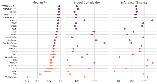
Figure 5: Performance comparison of TPSR and SRBench algorithms in terms of Accuracy-Complexity-Time on Feynman (top) and Black-box (bottom) datasets. For Feynman dataset, algorithms are sorted based on mean accuracy defined as the ratio of solutions with $R^{2}>0.99$ on test set under various noise levels, and for Black-box dataset, the algorithms are sorted based on the median $R^{2}$ score on test set. TPSR demonstrates a strong balance of performance with relatively low model complexity and lower inference time compared to GP-based algorithms. The error bars represent the 95% confidence interval and "$*$" refers to SR methods for Black-box dataset.

As shown in Table 1, when $\lambda=0$, the framework generates complex equations that overoptimize for fitting performance. However, as we increase $\lambda$, the framework generates less complex equations with a slight reduction in fitting performance. Notably, even for large values of $\lambda$, such as $\lambda=1$, the fitting performance of TPSR significantly outperforms that of the baseline methods. Based on the results, we recommend a default setting of $\lambda=0.1$ as it offers a balanced trade-off between complexity and accuracy, while also mitigating potential overfitting (as detailed in Appendix D.1). These findings demonstrate the superiority of TPSR over the baseline methods in terms of fitting performance across all datasets, while generating equations with comparable or reduced complexity than those generated by the baseline methods. Table 1 shows that TPSR exhibits a more significant gap in fitting performance when compared to E2E baselines on SRBench datasets, while this gap is smaller for In-domain datasets (even performing slightly worse on $\mathrm{\textit{Acc}}_{\omega}$ for larger $\lambda=0.5,1$). This is due to the In-domain dataset being generated using the same approach as the E2E pre-training data, resulting in the E2E model’s superior performance on this synthetic dataset. Furthermore, qualitative comparisons of TPSR with baseline symbolic and black-box regression models [47] demonstrate the superior performance of TPSR in learning the underlying equation and out-of-domain extrapolation (see Appendix D.2).

Fig. 5 presents a detailed comparison of our proposed TPSR with the baseline E2E transformer model and all the SRBench baselines on the PMLB Feynman and Black-box datasets. This figure illustrate the relative position of each algorithm with respect to (1) fitting performance, (2) model complexity, and (3) inference time. The results indicate that transformer-based planning in the TPSR significantly enhances the performance of E2E and outperforms even the state-of-the-art GP baselines, achieving the highest fitting performance on the black-box datasets. This is achieved while the complexity of the generated equations in TPSR is not greater than that of E2E, and shows a great fitting-complexity balance compared to other SR algorithms. The pareto plots provided in Fig. 1 also demonstrate the effectiveness of TPSR in balancing fitting and complexity compared to all other SRBench baselines. Our TPSR effectively pushes this balanced performance to the first pareto front for both the Feynman and Black-box datasets. Moreover, it is important to note that, while the inference time of TPSR is longer than the baseline E2E transformer model, it still has significantly lower inference time than RL or GP-based SRBench baselines. Further results on the SRBench and In-domain datasets are provided in Appendix D.

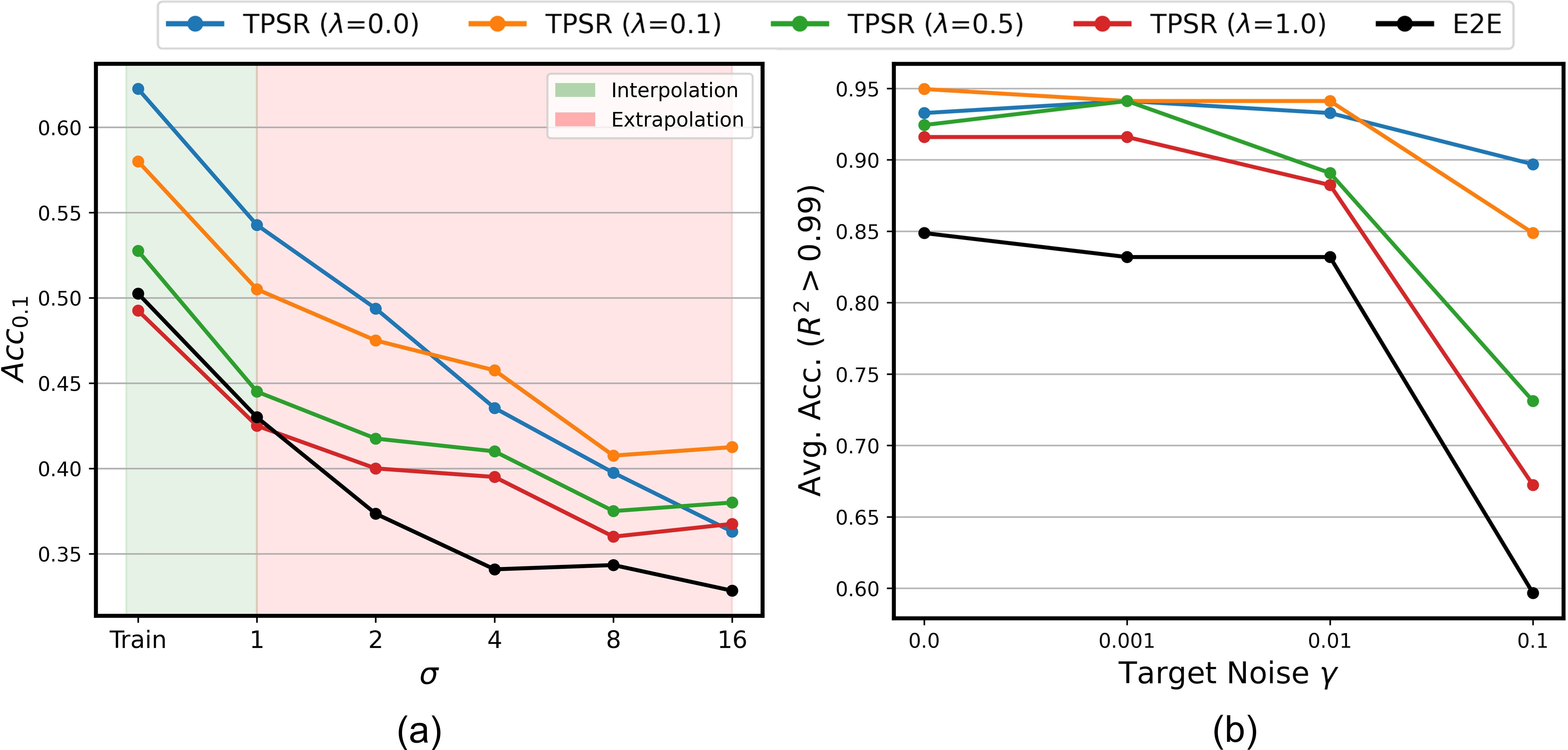
Figure 6: TPSR with $\lambda\in\{0,0.1,0.5,1\}$ compared to E2E for (a) Extrapolation performance where in-domain accuracy is shown for different input variances ($\sigma$), and (b) Robustness to noise, where mean accuracy ($R^{2}>0.99$) is shown for various target noise levels ($\gamma$).

4.4 (RQ2) Extrapolation and Robustness

The ability to extrapolate well is inherently linked to the quality of the equation obtained through symbolic regression. To investigate the extrapolation performance of TPSR to out-of-training regions, we normalize the input test data points to different scales ($\sigma$) instead of unit variance (used for training points) as per [18]. Fig. 6(a) depicts the average performance of TPSR compared to E2E with sampling decoding on the training data as well as testing data in scales of $\sigma\in\{1,2,4,8,16\}$ for the In-domain Synthetic dataset. Also, we investigate the effect of different complexity controlling levels ($\lambda\in\{0,0.1,0.5,1.0\}$) on the extrapolation performance. It can be observed that, while $\lambda=0$ (i.e., no complexity regularization) achieves the best fitting accuracy on the training data, it has a sub-par performance for $\sigma>8$. This can be due to the overfitting issue when the symbolic model is much more complex than the real complexity of the equation, similar to the common overfitting issue in ML models. The results highlight the importance of controlling complexity in the extrapolation of identified equations. For values of $\lambda>0$, the overfitting issue is mitigated as the generated equations become less complex. However, very high values of $\lambda$ (e.g., $\lambda=1$) can result in poor fitting performance. The flexibility of TPSR for allowing different values of $\lambda$ to balance fitting and complexity for a given task is crucial for optimal performance. Fig. 6(b) also presents the robustness of TPSR with different $\lambda$ levels compared to the E2E transformer baseline on the Feynman dataset. The results indicate that MCTS-guided decoding can offer robust performance with a smaller drop compared to the baseline in the presence of noise.

4.5 Ablation Study

In this section, we investigate the effect of different MCTS parameters and caching mechanisms on the performance of TPSR by conducting ablative experiments on the Feynman datasets.

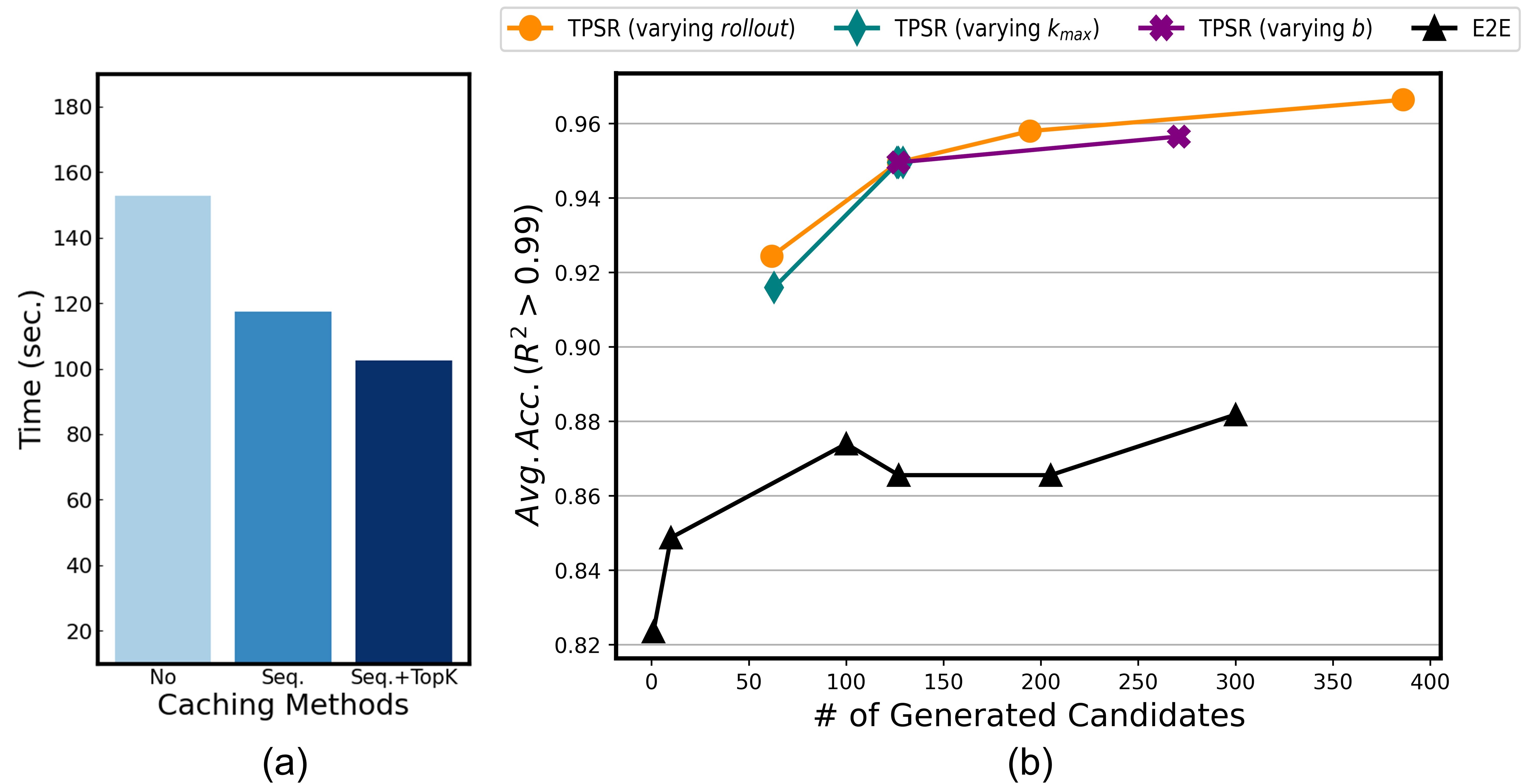
Figure 7: Ablation study on the modules and parameters of TPSR. (a) Effect of caching mechanisms: Sequence caching and $top$-$k$ caching improve the inference time of TPSR ($\lambda=0.1$). (b) Efficiency and parameters of TPSR: Average accuracy of TPSR (varying model parameters), and baseline E2E (varying sampling size) vs. number of generated candidates.

(RQ3) Caching Mechanisms. In Fig. 7(a), we illustrate the effectiveness of the sequence and $top$-$k$ caching mechanisms in reducing the total inference time of TPSR ($\lambda=0.1$). Our experiments show that sequence caching has more effect in dropping the inference time as it replaces the time-consuming sequence generation process. Overall, these two mechanisms can reduce the total inference time by around $28\%$.

(RQ4) Search Parameters. Fig. 7(b) shows the fitting performance against the number of generated equations during the decoding process for both TPSR ($\lambda=0.1$) and the baseline E2E with sampling decoding. In this figure, the ‘number of generated equation candidates’ represents the total number of complete equation sequences generated by each method. Specifically, this refers to the sample size in the E2E with sampling decoding, and the function calls of the beam search sub-routine multiplied by beam size $b$ in TPSR. The results show that under the same number of generated equation candidates, TPSR significantly outperforms the E2E baseline. This is primarily attributed to the fact that the E2E baseline is deprived of any feedback on the fitting performance of the generated equations. We report the results for variants of TPSR with different MCTS parameters. We assess the performance with varying number of rollouts, $r=\{1,3,6,9\}$, number of beams in simulations, $b=\{1,3\}$, and the maximum number of possible expansions at each state, $k_{max}=\{2,3,4\}$. The default setting of TPSR parameters are $b=1$, $k_{max}=3$, and $r=3$. The results indicate that increasing $r$, $k_{max}$, and $b$ all contribute to the better performance of TPSR, with the most significant improvement observed when increasing $r$. This is because more rollouts provide the model with more opportunities to learn from trials and learn better values.

5 Conclusion

In this work, we propose TPSR, a model-agnostic decoding strategy for symbolic regression that leverages the power of pre-trained SR transformer models combined with MCTS lookahead planning, and outperforms the existing methods in generating equations with superior fitting-complexity trade-off. We demonstrate the flexibility of TPSR in controlling equation complexity without fine-tuning the pre-trained model. Results also show that better expressions obtained with lookahead planning can further improve model performance in terms of noise robustness and extrapolation to unseen data. Future research could focus on enhancing the adaptability of feedback-based expression generation mechanisms, potentially by modulating the flexibility of MCTS or SR model weights, and the integration of MCTS with the training or fine-tuning of transformer SR models. Furthermore, employing parallelization and distributed computing could potentially improve MCTS search efficiency.

Appendix

Appendix A Dataset Details

We evaluate TPSR and several baseline methods on the following four standard benchmark datasets: Feynman, Black-box, and Strogatz from SRBench [42], and In-domain Synthetic Data generated based on [18]. More details on each of these datasets are given below.

• Feynman: This dataset contains $119$ equations sourced from Feynman Lectures on Physics database series [44]. The regression input points $(x,y)$ from these equations are provided in Penn Machine Learning Benchmark (PMLB) dataset [42, 43] and have been studied in SRBench [42] for the symbolic regression task. The input dimension is limited to $d\leq 10$ and the true underlying function of points is known. We split the dataset into $B$ bags of $200$ input points (when $N$ is larger than $200$) since the transformer SR model is pretrained on $N\leq 200$ input points as per [18].

• Strogatz: This dataset comprises $14$ symbolic regression problems sourced from the ODE-Strogatz database [45] for nonlinear dynamical systems. The input points for these problems are included in PMLB [43] and have been examined in SRBench [42] for symbolic regression. The input dimension for these problems is restricted to $d=2$ and the true underlying functions are provided.

• Black-box: The black-box regression datasets from PMLB [43] are used for the symbolic regression task and studied in SRBench [42] among various baselines. The aim of SR study on these black-box datasets is to find an interpretable model expression that fits the data effectively. We limit the datasets to those with continuous features and input dimension $d\leq 10$, as the transformer SR model [18] is pretrained with $d_{max}=10$. In total, there are $57$ black-box datasets that consist of real-world and synthetic datasets with varying levels of noise.

• In-domain Synthetic Data: Following [18], we construct a fixed validation set consisting of $400$ equation examples in which the validation functions were uniformly distributed across three different difficulty factors: input dimension ($d$), number of unary operators ($u$), and binary operators ($b$). Specifically, we set $d\sim\mathcal{U}(1,d_{max})$, $b\in\mathcal{U}(d-1,d+b_{max})$, and $u\sim\mathcal{U}(0,u_{max})$, where $d_{max}=10$, $u_{max}=5$, and $b_{max}=5+d$. The equation sequence is generated for each function by providing $N=[50,100,150,200]$ input points $(x,y)$, and the prediction accuracy is assessed on $N_{test}=200$ points that are randomly extracted from a multimodal distribution, as described in [18]. This data is referred to as “in-domain” because the validation data is generated using the same approach as the data on which the model [18] is pretrained.

Appendix B Implementation Details

Our model implementation leverages the state-of-the-art open-source End-to-End (E2E) SR model [18] as the pre-trained transformer backbone. This selection is due to the public availability of E2E’s model architecture, weights, and logits in the Facebook symbolicregression library and repository . The algorithm of our model is provided in Appendix C and the implementation code for our experiments with configuration details for reproducibility is available . In our experiments, the model’s maximum sequence length is set to $L=200$, and the constant to prevent numerical stability $\epsilon$ in NMSE calculation $(\frac{1}{n}\|y-\tilde{f}(\bm{x})\|_{2}^{2})/(\frac{1}{n}\|y\|_{2}^{2}+\epsilon)$ is set to $1e-9$. We set the default maximum number of node expansions ($k_{max}$) to be 3, the beam size of simulations ($b$) as 1, and the number of rollouts ($r$) as 3. The complexity-controlling parameter ($\lambda$) was also varied across four values: ${0,0.1,0.5,1}$. To ensure consistency with the protocol set out by [18], we divided the observation points of each equation in the SRBench datasets (including Feynman, Strogatz, and Black-box) into training and testing sets at a ratio of $75\%/25\%$. In the evaluation experiments involving In-domain Synthetic Data, we adjusted the number of observation points for each equation on which TPSR was trained to $N\in[50,100,150,200]$. The generated expression was subsequently tested on the $N_{test}=200$ data points for each sampling variance ($\sigma$) of 1, 2, 4, 8, and 16. These synthetic input points with varying sampling variance are introduced in In-domain data [18] to assess the models’ extrapolation capabilities under different conditions. All experiments are implemented with PyTorch on four Quadro RTX 8000 GPUs, with 48GB of RAM.

Table 2: Experimental Settings of TPSR and E2E [18]

Setting/Parameter	TPSR	E2E
Maximum Equation Length ($L$)	$200$	$200$
Maximum No. of Observations ($N$)	$200$	$200$
Maximum Input Dimension ($D$)	$10$	$10$
Maximum No. of Bags ($B$)	$10$	$10$
Beam/Sample size ($C$)	–	$10$
No. of Refinement Candidates ($K$)	–	$10$
Maximum Expansion Width ($k_{max}$)	$3$	–
Maximum No. of Rollouts ($r$)	$3$	–
Beam Size in Simulations ($b$)	$1$	–
UCT Exploration Parameter ($\beta$)	$1$	–

Appendix C Methodology Details

C.1 MCTS-Guided Decoding Details

Algorithm 1 provides the details of steps in MCTS-Guided decoding strategy for SR, following [37]. Here, the blue lines correspond to the utilization of reward and selection functions defined in Eqs. (2) and (1) of Section 3. These functions play a crucial role in guiding the MCTS-based Transformer Decoding strategy for SR and ensuring effective exploration and exploitation within the search space. Meanwhile, the red lines in the algorithm denote the places when the pre-trained transformer SR model is invoked to extract the $top$-$k$ next tokens and equation candidate beams. These extracted tokens and beams are employed in the expansion and evaluation steps of the MCTS algorithm, respectively. By incorporating the pre-trained transformer SR model, the MCTS-Guided decoding strategy can effectively leverage the model’s inherent semantic knowledge gained through large-scale pre-training to generate high-quality equation candidates and enhance the overall performance of the SR approach. Notably, in this MCTS setting, a "visit" signifies that a state-action pairing, $(s,a)$, has been explored during tree search, appending the corresponding child state, $s^{\prime}$, to the tree. Sequences that are generated as part of the beam search sub-routine of simulations in the evaluation stage of MCTS are not directly considered as visits to the nodes corresponding to these sequences. Instead, they serve the purpose of completing the partial equation to allow for feedback computation. As for cache hits, they are also not counted as visits. The reason is that caching in this context is used to save computation by storing previously computed values, and a cache hit simply means retrieving a stored value rather than performing a new visit.

Input :  $r_{max}$: maximum number of rollouts, $k_{max}$: number of children of nodes used for top-k next token selection, $b$: beam size, $c$: P-UCB exploration parameter

while $r<r_{max}$ do

       node $\leftarrow$ root;

       1) Selection

       while $|\textit{node.children}|>0$ do

             node $\leftarrow$ SELECT(node.children, $c$);

            

       end while

      2) Expansion

       next tokens $\leftarrow$ TOP_K(node, $k_{max}$);

       for action $\in$ next tokens do

             next state $\leftarrow$ CONCAT(node, action);

             Add next state as a child of node;

            

       end for

      3) Evaluation

       Equation $\leftarrow$ BEAM_SEARCH(node, $b$);

       reward $\leftarrow$ GET_REWARD(Equation);

       Save (Equation, reward) pair in a dictionary. ;

       4) Backpropagation

       Update values on the trajectory given the reward ;

      

end while

Return Equation with the highest reward ;

Algorithm 1 MCTS-Guided Decoding for Symbolic Regression

C.2 Distinguishing TPSR from other MCTS Approaches in SR

Figure 8: MCTS-Guided decoding algorithm for Symbolic Regression without using the pretrained transformer SR model for expansion and evaluation steps.

Figure 9: MCTS-Guided decoding algorithm for Symbolic Regression with the pretrained Transformer model used for expansion and evaluation steps.

It is essential to highlight that the implementation of the MCTS approach in TPSR differs from the standalone MCTS algorithm for SR. In a recent work, Sun et al. [26] shows that Monte Carlo Tree Search can be effective for exploring the optimal expression trees that govern nonlinear dynamical systems. This work introduces several adjustments to the conventional MCTS to enable the recovery of equations as expression trees. However, we would like to remark that using MCTS as a standalone algorithm for SR is a single-instance SR method, meaning that it requires searching from scratch for a new function or measurement data, and does not leverage pre-trained SR priors. To highlight the role of pre-trained transformer in our TPSR framework, we compare the MCTS-guided decoding algorithm in TPSR (Fig. 9, replicated from the main body for ease of comparison) with a standard MCTS algorithm (Fig. 8) which can be used in a similar fashion but without sharing information with the transformers. During the expansion phase, standard MCTS chooses the next accessible action from the action set (i.e., the vocabulary of tokens) and appends the state that can be reached through the chosen action. In this example, action $x_{1}$ is selected, and the new state appended to the tree is $[sin,x_{1}]$. Subsequently, during the evaluation phase, MCTS assesses the new state by implementing a random policy from the new state and calculating the policy’s value. Applying the standard MCTS algorithm to domains characterized by extensive state or action spaces, such as SR with a combinatorial optimization space that exponentially grows with the number of input variables, is highly impractical. This is because attempting all possible actions in the expansion phase is infeasible. Furthermore, the random policy employed in the evaluation phase exhibits significant variance when estimating the new state’s value, and may result in invalid equations that are unsuitable for proper evaluation (e.g., accurately assessing fitting performance). To overcome these limitations, TPSR employs the pre-trained Transformer SR model. This approach leverages the semantic knowledge embedded in large-scale pre-trained priors, while conducting lookahead planning to optimize equation generation for the equation discovery non-differentiable objectives. By integrating the pre-trained Transformer SR model, TPSR can effectively navigate the vast search space, reducing complexity and enhancing fitting performance, thus offering a more viable solution for the domain of SR.

It is also crucial to emphasize how the integration of MCTS in TPSR differentiates from others, particularly from works like Kamienny et al. [48], which also pairs MCTS with pre-trained Transformers. Key differentiators include:

General Approach. Unlike [48] that exploits a pre-trained mutation policy $M$ to generate the expression by following a series of mutations from an empty expression (root), TPSR follows the seq2seq approach of E2E [18] to generate the expression token-by-token. Consequently, TPSR uses the pre-trained E2E as its backbone but [48] pre-trains the mutation policy from scratch.

MCTS and Search Strategy. In [48], the search tree consists of full mathematical equations, with each node representing a distinct equation and edges corresponding to mutations between equations. In contrast, TPSR employs MCTS as a decoding strategy in the context of the transformer model. Each node in the search tree of TPSR represents the current state of generated tokens, potentially forming non-complete sequences, with edges corresponding to mathematical operators or variables. So, the search tree of [48] with “n” nodes includes “n” different equations, while the TPSR search tree includes partial decoded sequences, and completed equations only exist at the terminal nodes. This distinction inherently leads to major differences in selection, expansion, and back-propagation mechanisms within the MCTS algorithm.

Parameter Update and Learning. [48] utilizes MCTS to update and learn the distribution of mutations for a group of out-of-distribution datasets. The approach involves fine-tuning an actor-critic-like model to adjust the pre-trained model on a group of symbolic regression instances. On the other hand, TPSR uses the pre-trained transformer’s learned distribution to guide the expansion during the search process, without updating any specific parameters for in-domain or out-of-domain datasets (without fine-tuning). Consequently, the same settings and pre-trained model are applied to both in-domain and out-of-domain evaluations in TPSR.

Computation Time. [48] involves pre-training a mutation policy, a critic network, and performing fine-tuning stages for these networks, leading to significantly higher computation time (a limit of $24$hrs and $500$K equation candidate evaluations as stated in [48]). In contrast, TPSR has substantially lower computation time and the number of equation candidate evaluations, typically in the order of $10^{2}$ equations, taking approximately $10^{2}$ seconds (as shown in Fig. 5 and 7). This renders TPSR more suitable for applications where fast yet accurate equation discovery is critical.

C.3 Caching Details

In the evaluation phase of MCTS, a transformer model is employed to produce complete sequences from a given state. This procedure entails the creation of implicit tree structures that are used to carry out a beam search. The beam search involves determining the $top$-$k$ next tokens for the states visited during the generation process until the entire sequence is generated. These calculations will be needed in future MCTS iterations for two purposes: (1) to extract the $top$-$k$ next tokens during the expansion step of each state and (2) to generate the complete equation from a given state during the evaluation step. To avoid redundant computations and improve the efficiency of the framework, two caching mechanisms are used, namely $top$-$k$ caching and sequence caching.

Top-k caching is a mechanism that stores the computed top-k values for given states. For example, in Fig. 4 of the main paper, when evaluating the state $s=[+,\mathrm{sin}]$ in iteration $t$ of MCTS, the $top$-$k$ tokens are calculated for $s$ and its subsequent visited states (e.g., $[+,\mathrm{sin},x_{2}]$). These pairs of states and their corresponding $top$-$k$ values can be stored in a top-k cache. Consequently, if a state $s$ is visited again in a future iteration (e.g., visiting $s=[+,\mathrm{sin},x_{2}]$ in iteration $t+1$ of MCTS), the cached $top$-$k$ values are utilized instead of calling pretrained SR model again and retrieving the $top$-$k$ tokens from the forward pass of model.

Another mechanism employed to reduce redundant computations is sequence caching, which caches complete equations generated in a greedy manner. When the beam size in MCTS is one, the sequence is generated greedily for the given state in the evaluation step. This means that if any partial sequence of this equation is given, the same equation will be generated by the decoder. As a result, the generated equation in iteration $t$ can be used directly in future iterations if the state matches the stored equation partially. For instance, in Fig. 4 of the main paper, consider the equation $\tilde{f}:[+,\mathrm{sin},x_{2},\cdot,x_{1}]$ is generated for $s=[+,\mathrm{sin}]$ with $b=1$ in iteration $t$. Now, if in a later iteration (e.g., iteration $t+1$), the state to evaluate is $s=[+,\mathrm{sin},x_{2}]$, the iterative sequence generation process can be bypassed by directly using the sequence cache to predict the complete equation. It is essential to note that both of these caching strategies serve the same purpose of enhancing the framework’s efficiency without compromising its performance.

Appendix D Further Results and Visualization

D.1 Controlling the Fitting-Complexity Trade-off

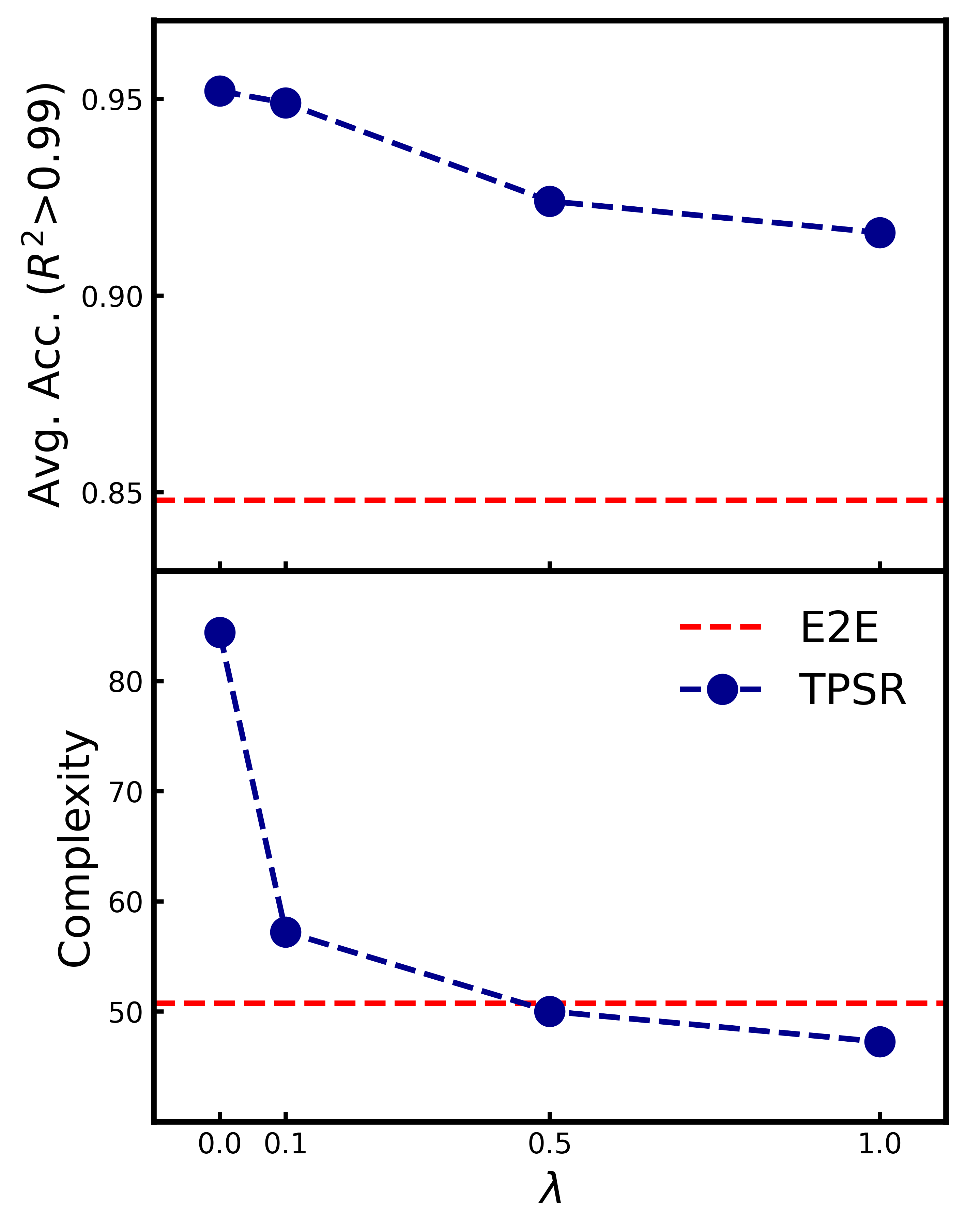
Figure 10: Effect of controllable complexity parameter ($\lambda$) on average test performance and equation complexity for the Feynman dataset. E2E uses sampling decoding.

Figure 10 illustrates the relationship between fitting accuracy and complexity of predicted equations for various values of $\lambda\in\{0,1,0.5,1\}$, on the Feynman dataset. This figure highlights the impact of the controllable complexity parameter $\lambda$ on balancing the trade-off between fitting performance and equation complexity. As it can be observed, when the value of $\lambda$ is set to $0$, the TPSR framework generates exceedingly complex equations, resulting in a complexity score greater than $80$. These equations are primarily focused on optimizing fitting performance. However, as $\lambda$ is slightly increased to $0.1$, there is a minimal effect on the fitting performance, while the complexity of the generated equations drops significantly to a score of less than $60$. As $\lambda$ continues to increase, the TPSR framework produces equations with reduced complexity, accompanied by a slight decline in fitting performance. Figure 10 demonstrates that even when $\lambda$ is set to a large value, such as $1$, the fitting performance of the equations generated by TPSR remains notably superior to the baseline E2E+Sampling method ($\bm{0.916}$ versus $\bm{0.848}$). Additionally, the complexity of the generated equations marginally improves ($\bm{47.24}$ compared to $\bm{50.73}$). This can be observed by examining the gap between the red and blue dashed lines in both the top and bottom sub-figures of Figure 10. These findings emphasize the advantages of the TPSR framework over the baseline methods in terms of fitting performance. At the same time, TPSR is capable of generating equations with either comparable or lower complexity than those produced by the baseline methods.

Given the significance of $\lambda$ in governing this trade-off, and to assist users in hyperparameter selection, we recommend setting $\lambda=0.1$ as a default. Based on our results, particularly Table. 1 and Fig. 10, we find that this setting tends to achieve a harmonious balance between accuracy and complexity, mitigating overfitting. It is important to note that this recommendation aims to offer a starting point for users. The appropriate choice of this hyperparameter may depend on the specific use case, where the balance between finding an accurate function and sacrificing complexity, versus emphasizing interpretability and equation simplicity over relative accuracy, becomes relevant.

Figure 11: Qualitative comparison of TPSR with E2E as well as black-box XGBoost [47] fitting. The training dataset contains 200 points in range of $(-2,2)$ (shaded region), and the performance is evaluated over $(-5,5)$. E2E uses sampling decoding.

D.2 Qualitative Study

Fig. 11 offers a detailed qualitative analysis comparing the performance of TPSR, the E2E baseline (symbolic model), and XGBoost [47] (black-box model) with respect to the ground-truth equation $x^{2}\mathrm{sin}(x)$. The training dataset, depicted by the shaded red region, consists of 200 data points randomly sampled within the range of $(-2,2)$. The evaluation is performed on an out-of-domain region spanning from $(-5,5)$.

While all three models demonstrate a strong ability to fit the training data, the proposed TPSR method surpasses the E2E baseline in fitting the true underlying function, as evidenced by its performance in the out-of-domain region. This superior performance can be attributed to TPSR’s capacity to generate less complex equations that still effectively fit the data, a feature highlighted in the accompanying complexity barplot. Moreover, the results showcase the general superiority of symbolic regression methods over the black-box XGBoost machine learning method when fitting the underlying function within the unseen evaluation range. This observation emphasizes the potential benefits of adopting symbolic regression techniques, such as TPSR, in providing more accurate representations of the data’s underlying patterns and behaviors.

D.3 Evaluating the Model-Agnostic Capability

In order to underscore the model-agnostic capabilities of TPSR, we also conducted evaluation experiments to include the integration of TPSR with the "Neural Symbolic Regression that Scales" (NeSymReS) model by Biggio et al. [16], a pioneering work for large-scale pre-training in SR.

Limitations and Adjustments. NeSymReS, while influential, presents some inherent limitations: (1) Dimensionality Constraint: It can only handle datasets having a maximum of three dimensions ($D\leq 3$). This limits its application in wider experimental scenarios. (2) Skeleton Prediction: NeSymReS is also trained to only predict equation skeletons. As such, the system requires a more complex constant optimization process, further complicating its integration.

Experiment Setup. Due to the constraints highlighted above, to evaluate the combination of TPSR with NeSymReS, we use a dataset composed of $52$ Feynman equations, as in [16], ensuring the dimensionality constraint ($D\leq 3$) is respected.

Results. As illustrated in Table 3, integrating TPSR with NeSymReS resulted in marked improvement. Specifically, results show that TPSR has significantly improved the fitting accuracy of NeSymReS without changing the average complexity of the equations when $\lambda=0.1$ and with a slight increase when $\lambda=0$.

Table 3: Fitting accuracy and complexity performance of NeSymReS [16] with and without the proposed TPSR planning on $52$ Feynman datasets with $D\leq 3$.

Model	Avg. ($R^{2}>0.99$) $\uparrow$	Avg. Complexity $\downarrow$
NeSymReS	0.635	9.98
NeSymReS+TPSR ($\lambda$=0.1)	0.808	9.98
NeSymReS+TPSR ($\lambda$=0)	0.827	13.30

D.4 Additional SRBench Results

Strogatz Datasets.

Figure 12 presents a performance comparison of TPSR and SRBench algorithms on the Strogatz dataset (similar to the results shown for Feynman and Black-box datasets in Fig. 5). The Strogatz dataset comprises 14 equations from a two-state system following a first-order ordinary differential equation (ODE). As it can be observed, E2E performance is less well on this dataset compared to other GP-based models due to the unique time-ordered distribution of observations, which differs substantially from the E2E’s pre-training data. Notably, despite not being exposed to time-ordered data during pre-training, TPSR with the E2E pre-training backbone significantly enhances its performance on the Strogatz dataset. TPSR ranks among the top three baselines for fitting performance while maintaining comparable or even slightly superior levels of equation complexity and inference time.

Figure 12: Performance comparison of TPSR and SRBench algorithms in terms of Accuracy-Complexity-Time on Strogatz dataset. Models are sorted based on mean accuracy defined as the ratio of solutions with $R^{2}>0.99$ on test set under various noise levels. The error bars represent the $95\%$ confidence interval.

Black-box Datasets.

SRBench [42] studied black-box problems, originally extracted from OpenML and integrated into PMLB [43] datasets, include several datasets derived from Friedman’s [49] synthetic benchmarks. These Friedman datasets, generated through non-linear functions, display varying degrees of noise, variable interactions, and non-linearity. As observed in earlier studies [42], the results from the Friedman datasets tend to highlight the performance differences among top-ranked methods more noticeably than other benchmarks, where top-performing methods often deliver similar results. Fig. 13 shows that performance of several baselines such as KernelRidge, MLP, DSR, BSR, gplearn, and AFP, degrades on Friedman datasets. However, our TPSR variants maintains its superior performance across these challenging Friedman synthetic datasets and the remaining PMLB black-box datasets, asserting its state-of-the-art (top-$1$) status. Following [42], this performance distinction is illustrated in Fig. 13 with more details, separating the results of Friedman datasets from the rest of PMLB datasets.

Figure 13: Detailed performance comparison of TPSR and SRBench algorithms in terms of Accuracy (Fitting Performance) on Black-box dataset groups: (1) Friedman [49] synthetic datasets, (2) non-Friedman datasets, and (3) all the black-box datasets. The error bars represent $95\%$ confidence interval and $"*"$ refers to SR methods vs. other ML methods.

Fig. 14 shows an in-depth comparison of TPSR performance, varying $\lambda\in{0,0.1,0.5,1}$, against top competitors (Operon, SBP-GP, FEAT, EPLEX, and E2E) on Black-box datasets of different input dimensions. Given E2E’s pre-training on $d_{max}\leq 10$, we focused on datasets with input dimensions below 10. In Fig. 14(a), we note that dataset distribution and model performance both depend on the input dimensionality. TPSR consistently outperforms competitors across most dimensions. Interestingly, lower dimensions (e.g., $d=3$) favor TPSR with higher $\lambda=0.5,1$, resulting in better performance, while larger dimensions (i.e., $d=8,9$) benefit from smaller $\lambda=0,0.1$. This pattern aligns with the expectation that greater $\lambda$ values yield less complex expressions, more prevalent in lower dimensions, and vice versa. Fig. 14(b) presents the average inference time for each model across different input dimensions. E2E is the fastest, while SBP-GP and DSR are the slowest. Notably, as input dimension increases, the inference time of Operon and EPLEX significantly escalates, hitting the scale of $10^{4}$ and $10^{5}$ seconds respectively, while TPSR’s time remains relatively constant, peaking at $10^{3}$ seconds or roughly 30 minutes for $d=9$, compared to Operon’s 3 hours and SBP-GP’s 30 hours. This shows how efficient TPSR is compared to GP methods in finding state-of-the-art best-fitting expressions. Finally, Fig. 14(c) shows the average complexity of expressions generated by each model for different input dimensions. DSR’s expressions are the least complex, while SBP-GP’s are the most. TPSR with $\lambda=0$ is slightly more complex than its counterparts. Interestingly, TPSR with $\lambda=0.5,1$ produces less complex expressions than GP-based models like Operon, FEAT, and EPLEX at lower dimensions. However, as dimensions increase, these models generate less complex expressions than those of TPSR.

Figure 14: Detailed performance comparsion of TPSR and competing baselines in terms of Accuracy-Complexity-Time metrics for Black-box datasets of varying input dimensions.

D.5 Additional In-Domain Results

Fig. 15 presents a comprehensive performance comparison between our proposed TPSR method with varying controllable parameter $\lambda\in{0,0.1,0.5,1}$ and the E2E baseline employing sampling for the In-domain Synthetic Dataset. As observed, when the complexity of the synthetic formula increases (as shown in the top row), such as increasing the number of binary/unary operators or the input dimension, the performance across all models tends to degrade. However, we can see that TPSR with $\lambda=0,0.1$ “always“ have lower performance drops and TPSR with $\lambda=0.5,1$ “mostly“ have lower performance drop than the E2E. This highlights that not only does the incorporation of performance feedback in TPSR’s MCTS-guided decoding help the transformer generation scale better with these difficulty levels, but the controllable complexity parameter $\lambda$ also plays a pivotal role in performance scaling for more challenging input functions.

Fig. 15(d) illustrates that the performance of all models increases as the number of input data points $N$ grows, as one would expect. However, TPSR with $\lambda=0,0.1$ exhibits considerably better low-resource performance for $N<100$ compared to the E2E model. It is important to note that the maximum $N_{max}=200$ since the E2E model is pretrained with $N\leq 200$, and the transformer architecture employed in the encoding stage demands significant computational and GPU resources for training the model with $N>200$.

Fig. 15(e) also reveals that the performance of all models improves as the number of input data centroids increases, meaning that as the input data is sampled with greater diversity across different distribution clusters. We can clearly observe that our proposed TPSR with $\lambda=0,0.1$ consistently outperforms the E2E model, both with smaller and larger numbers of centroids.

Fig. 15(f) further investigates the impact of introducing multiplicative noise with variance $\gamma$ to the target $y$: $y\rightarrow y(1+\sigma),\sigma\sim\mathcal{N}(0,\gamma)$. As evident from the figure, the performance of all models deteriorates as the noise variance increases. This phenomenon highlights the sensitivity of the pretrained models to the input noise of the target variable. However, it is noteworthy that TPSR with $\lambda>0$ demonstrates slightly better performance compared to the E2E model, particularly when encountering larger noise variances.

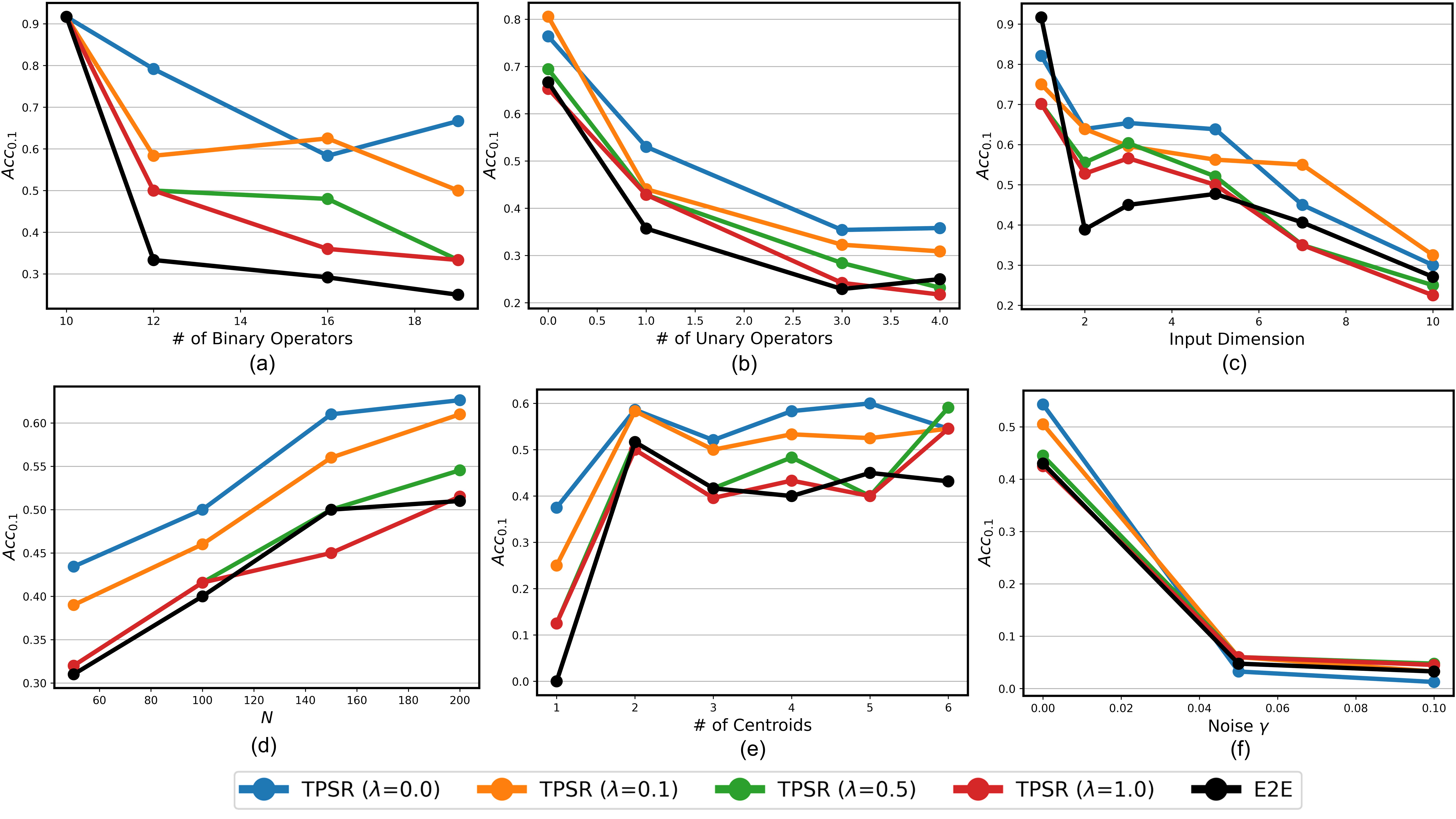
Figure 15: Performance comparison of TPSR for varying $\lambda\in\{0,0.1,0.5,1\}$ and E2E with sampling across different levels of formula and input difficulties: (a) number of binary operators, (b) number of unary operators, (c) input dimension, (d) number of input points $N$ (e) number of input centroids, and (f) input noise variance $\gamma$.

D.6 Additional Ablation Studies

The selection of $\beta$, in Eq. 1 can also affect the exploration-exploitation trade-off, influencing the overall performance of TPSR. Fig. 16 demonstrates the impact of varying $\beta$ on TPSR’s performance over $119$ Feynman datasets, emphasizing the balance between exploration and exploitation. Based on the results, we observe that for small values of $\beta$, specifically $\beta=0$, the performance is sub-optimal. This diminished performance can be attributed to constrained exploration. Without sufficient exploration, the model might miss potential solutions or equation sequences that might be more effective. At the other end of the spectrum, with large values like $\beta=100$, there is also a decline in performance. This degradation can be linked to an over-emphasis on exploration at the cost of exploitation. By exploring too much without adequately leveraging the learned knowledge, the model can get overwhelmed with possibilities, some of which might not be beneficial. Experiment results highlight that optimal performance is achieved for $\beta$ values ranging between 0.1 and 10. As seen in Fig. 16(b), with an increase in $\beta$, the number of equation sequence candidates grows, indicating an increase in exploration. However, beyond $\beta>0.1$, the increase in sequence candidates is marginal. This plateau suggests the possible activation of caching mechanisms due to repetitive sequence generation. Fig. 16(a) also shows fitting performance against different $\beta$ values, illustrating the aforementioned trends and offering a visual guide for selecting $\beta$.

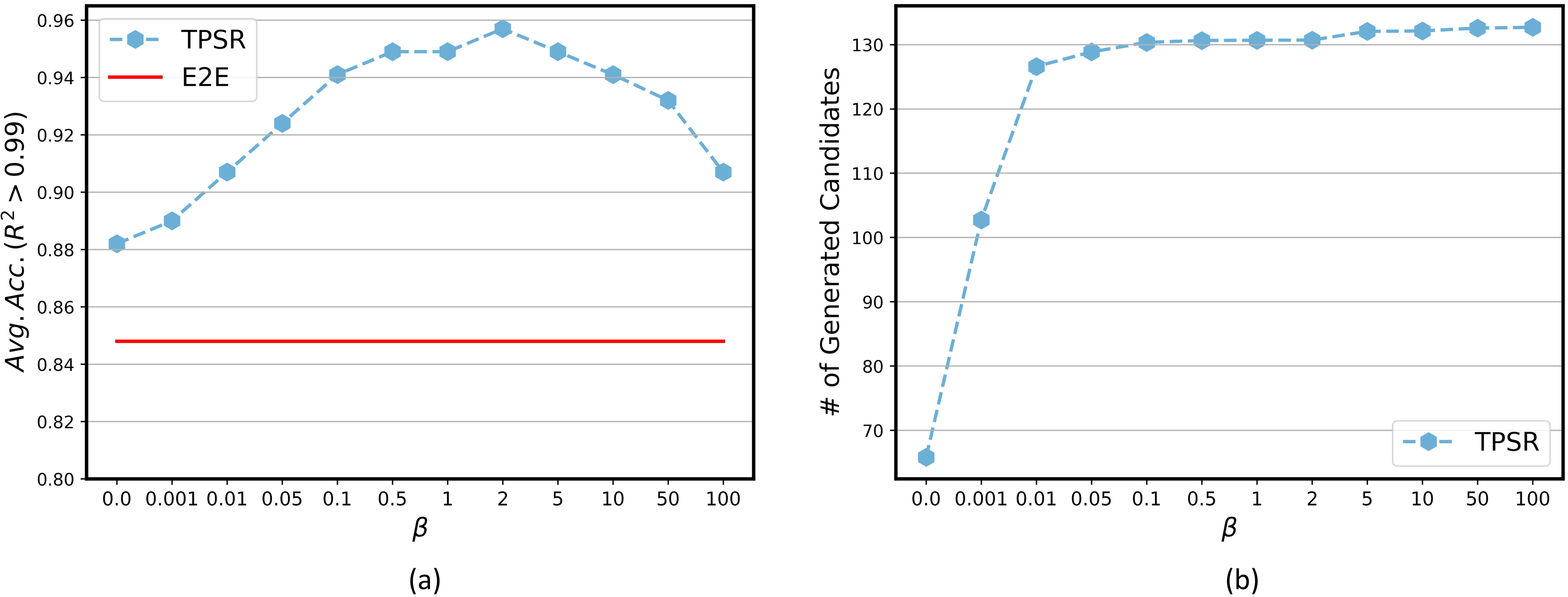
Figure 16: Ablation study of $\beta$ on TPSR using $119$ Feynman datasets: Balancing Exploration and Exploitation.

Table 4: Example comparisons of symbolic expressions generated by E2E and TPSR, along with their respective fitting performance.

	Expression	$R^{2}$
True Function	$2X_{0}(1-\cos{(\bm{X_{1}X_{2}})})$	–
E2E Generation	$CX_{0}\left(C+C\cos{\left(CX_{2}+CX_{1}\right)}\right)+C$	0.453
TPSR Generation	$CX_{0}\left(C+C\cos{\left(CX_{1}+CX_{2}\bm{+CX_{1}X_{2}}\right)}\right)+C$	1.0
True Function	$\bm{\sin^{2}}{\left(\frac{\bm{X_{0}X_{1}}}{\left(\frac{\bm{X_{2}}}{2\pi}\right)}\right)}$	–
E2E Generation	$C\sin{\left(CX_{0}+CX_{1}+CX_{2}\right)}+C$	0.178
TPSR Generation	$C\bm{\sin^{2}}{\left(\frac{\bm{CX_{1}X_{0}}}{\bm{CX_{2}}+CX_{1}}\right)}+C$	0.671
True Function	$X_{0}\left(\cos{\left(\bm{X_{1}X_{2}}\right)}+\bm{X_{3}}\bm{\cos^{2}{\left(X_{1}X_{2}\right)}}\right)$	–
E2E Generation	$CX_{0}\left(CX_{3}+CX_{2}+CX_{1}+C\cos{\left(CX_{2}+CX_{1}\right)}\right)^{2}+C$	0.878
TPSR Generation	$CX_{0}\left(\cos{\left(\bm{CX_{2}X_{1}}\right)}+X_{3}^{2}\cos^{2}{\left(\bm{CX_{2}X_{1}}\right)}\right)+C$	0.996
True Function	$X_{0}\frac{\bm{\sin^{2}}{(\frac{\bm{X_{1}X_{2}}}{2})}}{\bm{\sin^{2}}{(\frac{\bm{X_{2}}}{2})}}$	–
E2E Generation	$CX_{0}+CX_{0}\left(C\sin{\left(CX_{1}+CX_{2}\right)}+CX^{2}_{1}\right)^{2}+C$	0.655
TPSR Generation	$CX^{2}_{0}\bm{\left(\frac{\sin{\left(CX_{2}X_{1}\right)}}{\sin{\left(CX_{2}\right)}}\right)^{2}}+C$	0.991
True Function	$\sqrt{\left(X^{2}_{0}+X^{2}_{1}-2X_{0}X_{1}\cos{\left(\bm{X_{2}-X_{3}}\right)}\right)}$	–
E2E Generation	$\sqrt{\left(CX_{0}+CX_{1}\right)^{2}\cos{\left(CX_{2}+CX^{2}_{3}\right)}}+C$	0.939
TPSR Generation	$\sqrt{\left(CX_{1}X_{0}\cos{\left(\bm{CX_{2}-CX3}\right)}-CX^{2}_{1}X^{2}_{0}\right)}+C$	0.986

D.7 Examples of Generated Symbolic Expressions

Table 4 presents example comparisons of symbolic expressions generated by E2E using sampling and our proposed TPSR model with $\lambda=1$ for 200 observation points of given true functions. To improve readability and simplify notation, all constants in the generated expressions are denoted with the token “C“. The table highlights how TPSR-generated symbolic expressions are more closely aligned with the true functions than those generated by E2E. The aligned components are bolded in the table entries. Additionally, the fitting performance $R^{2}$ of TPSR-generated equations is notably superior to that of E2E-generated expressions. This comparison demonstrates how TPSR’s integration of feedback in transformer decoding can yield quantitatively and qualitatively improved expressions using the same model weights. Improved learning of expressions behind the data can enhance the interpretability of black-box prediction models, contributing to their extrapolation and generalizability.

Appendix E Discussion and Future Work

Limitations.

While our methodology exhibits substantial potential, it is not without limitations. One limitation of our approach is the increased inference time of the TPSR in comparison to simpler decoding methods like beam search and sampling. This extended inference time is primarily due to the process of searching and incorporating performance feedback during the generation phase in TPSR’s decoding process. Nevertheless, by exploiting the semantic knowledge of large-scale pre-trained SR model, TPSR’s inference time remains lower than the majority of GP-based SRBench baselines. Another factor influencing TPSR’s performance is the dependency on the learned priors of the pre-trained SR model. TPSR is also subject to the inherent structural limitations of the pre-trained SR model, such as constraints on input dimensionality, expression length, and vocabulary definition. For example, the E2E model is pre-trained with a maximum input dimension ($d_{max}$) of 10, which in turn limits the TPSR with the E2E backbone to $d\leq 10$. However, it’s important to note that TPSR is a model-agnostic framework, implying potential integration with more advanced pre-trained SR models in the future.

Future Directions.

An intriguing dimension in the symbolic regression revolves around out-of-distribution data. Pre-trained Transformer SR methods, distinct from their search-focused counterparts, train on vast synthetic equation datasets stemming from certain distributions. Essentially, this distribution is shaped by specific equation generators and sampling techniques. Hence, any data or equation not stemming from these generators could be viewed as out-of-distribution. Our experimentation evaluated TPSR and the pre-trained E2E model [18] across both in-domain and out-of-distribution datasets, as in the SRBench. A crucial observation was that TPSR, with lookahead planning, considerably elevates the pre-trained model’s performance on out-of-distribution datasets, a trend most pronounced in SRBench comparisons (as illustrated in Table 1). While pre-trained models offer the strength of utilizing prior knowledge from large-scale datasets, they can be limited when faced with data far removed from their training distribution or unique equation forms they have not encountered during training. TPSR offers a partial solution through its decoding-stage search and planning, but it is still limited to the inherent constraints of the pre-trained SR model’s priors. Addressing this challenge is an intriguing avenue for future research. Possible strategies might involve fine-tuning SR model weights using non-differentiable rewards for the new out-of-distribution datasets.

Appendix F Broader Impacts

Potential positive impacts.

The proposed TPSR approach for symbolic regression using transformer-based models has significant implications for both the research and practical communities. By integrating Monte Carlo Tree Search (MCTS) into the transformer decoding process, TPSR enables the generation of equation sequences that balance fitting accuracy and complexity, addressing key challenges in symbolic regression. This has wide-ranging applications in science and engineering domains, where accurate and interpretable mathematical models are essential for understanding and predicting complex phenomena. The improved performance of TPSR over state-of-the-art methods enhances the usability and reliability of symbolic regression models, enabling researchers and practitioners to extract valuable insights from their data and make informed decisions.

Moreover, TPSR offers practical benefits by leveraging the efficiency of transformer-based models and the pretraining priors. The ability to optimize equation generation using TPSR enhances the efficiency and scalability of symbolic regression, making it more accessible in resource-constrained settings. This opens up opportunities for the adoption of symbolic regression in various domains, including scientific research, engineering design, and optimization problems. The impact of TPSR extends beyond symbolic regression, as the integration of MCTS and non-differentiable feedback into transformer-based models can inspire novel approaches in other fields where the combination of symbolic reasoning and machine learning is valuable. Overall, TPSR has the potential to advance the state-of-the-art in symbolic regression and contribute to scientific and technological advancements.

Ethical considerations.

Symbolic regression makes it easier for anyone to understand underlying patterns behind the data and learn interpretable symbolic mathematical models for observations. This approach brings the potential for machine learning models to achieve a balance of high predictive performance and transparency, which is critically valuable in sectors such as healthcare, where the interpretability of models can directly influence life-saving decisions. However, as with any powerful tool, the ethical issues of its use must be considered carefully. For example, while symbolic regression can yield life-saving insights in the hands of healthcare professionals, it can also be exploited for malicious purposes. It could be used to decipher patterns and relationships within data where privacy should be maintained, leading to potential breaches of confidentiality. This becomes particularly concerning as symbolic regression techniques mature, enabling more effective comprehension of symbolic mathematical relationships behind data values. To mitigate this risk, we need the development of a separate modules tasked with screening input data and denying requests where pattern extraction could lead to harmful outcomes.

References

- [1] He Ma, Arunachalam Narayanaswamy, Patrick Riley, and Li Li. Evolving symbolic density functionals. Science Advances, 8(36):eabq0279, 2022.
- [2] Yiqun Wang, Nicholas Wagner, and James M. Rondinelli. Symbolic regression in materials science. MRS Communications, 9(3):793–805, 2019.
- [3] Samuel H. Rudy, Steven L. Brunton, Joshua L. Proctor, and J. Nathan Kutz. Data-driven discovery of partial differential equations. Science Advances, 3(4):e1602614, 2017.
- [4] Kazem Meidani and Amir Barati Farimani. Data-driven identification of 2d partial differential equations using extracted physical features. Computer Methods in Applied Mechanics and Engineering, 381:113831, 2021.
- [5] Steven L. Brunton, Joshua L. Proctor, and J. Nathan Kutz. Discovering governing equations from data by sparse identification of nonlinear dynamical systems. Proceedings of the National Academy of Sciences, 113(15):3932–3937, 2016.
- [6] Miles Cranmer, Alvaro Sanchez-Gonzalez, Peter Battaglia, Rui Xu, Kyle Cranmer, David Spergel, and Shirley Ho. Discovering symbolic models from deep learning with inductive biases. In Proceedings of the 34th International Conference on Neural Information Processing Systems, NIPS’20, Red Hook, NY, USA, 2020.
- [7] E. Kaiser, J. N. Kutz, and S. L. Brunton. Sparse identification of nonlinear dynamics for model predictive control in the low-data limit. Proceedings of the Royal Society A: Mathematical, Physical and Engineering Sciences, 474(2219):20180335, 2018.
- [8] Kazem Meidani and Amir Barati Farimani. Identification of parametric dynamical systems using integer programming. Expert Systems with Applications, 219:119622, 2023.
- [9] Yoshitomo Matsubara, Naoya Chiba, Ryo Igarashi, Taniai Tatsunori, and Yoshitaka Ushiku. Rethinking symbolic regression datasets and benchmarks for scientific discovery. arXiv preprint arXiv:2206.10540, 2022.
- [10] Marco Virgolin and Solon P Pissis. Symbolic regression is NP-hard. Transactions on Machine Learning Research, 2022.
- [11] Haoran Li, Yang Weng, and Hanghang Tong. CoNSole: Convex neural symbolic learning. In Alice H. Oh, Alekh Agarwal, Danielle Belgrave, and Kyunghyun Cho, editors, Advances in Neural Information Processing Systems, 2022.
- [12] Michael Schmidt and Hod Lipson. Distilling free-form natural laws from experimental data. Science Advance, 324(5923):81–85, 2009.
- [13] Bogdan Burlacu, Gabriel Kronberger, and Michael Kommenda. Operon c++: An efficient genetic programming framework for symbolic regression. In Proceedings of the 2020 Genetic and Evolutionary Computation Conference Companion, GECCO ’20, page 1562–1570, New York, NY, USA, 2020. Association for Computing Machinery.
- [14] Brenden K Petersen, Mikel Landajuela Larma, Terrell N. Mundhenk, Claudio Prata Santiago, Soo Kyung Kim, and Joanne Taery Kim. Deep symbolic regression: Recovering mathematical expressions from data via risk-seeking policy gradients. In International Conference on Learning Representations, 2021.
- [15] Ashish Vaswani, Noam Shazeer, Niki Parmar, Jakob Uszkoreit, Llion Jones, Aidan N Gomez, Ł ukasz Kaiser, and Illia Polosukhin. Attention is all you need. In Advances in Neural Information Processing Systems, volume 30, 2017.
- [16] Luca Biggio, Tommaso Bendinelli, Alexander Neitz, Aurelien Lucchi, and Giambattista Parascandolo. Neural symbolic regression that scales. In Marina Meila and Tong Zhang, editors, Proceedings of the 38th International Conference on Machine Learning, volume 139 of Proceedings of Machine Learning Research, pages 936–945. PMLR, 18–24 Jul 2021.
- [17] Mojtaba Valipour, Bowen You, Maysum Panju, and Ali Ghodsi. Symbolicgpt: A generative transformer model for symbolic regression. arXiv preprint arXiv:2106.14131, 2021.
- [18] Pierre-Alexandre Kamienny, Stéphane d’Ascoli, Guillaume Lample, and Francois Charton. End-to-end symbolic regression with transformers. In Advances in Neural Information Processing Systems, 2022.
- [19] Martin Vastl, Jonáš Kulhánek, Jirí Kubalík, Erik Derner, and Robert Babuška. Symformer: End-to-end symbolic regression using transformer-based architecture. arXiv preprint arXiv:2205.15764, 2022.
- [20] Alex Graves. Sequence transduction with recurrent neural networks. arXiv preprint arXiv:1211.3711, 2012.
- [21] Sam Wiseman and Alexander M. Rush. Sequence-to-sequence learning as beam-search optimization. In Proceedings of the 2016 Conference on Empirical Methods in Natural Language Processing, pages 1296–1306, Austin, Texas, November 2016. Association for Computational Linguistics.
- [22] Angela Fan, Mike Lewis, and Yann Dauphin. Hierarchical neural story generation. In Proceedings of the 56th Annual Meeting of the Association for Computational Linguistics (Volume 1: Long Papers), pages 889–898, Melbourne, Australia, jul 2018. Association for Computational Linguistics.
- [23] Allan Costa, Rumen Dangovski, Owen Dugan, Samuel Kim, Pawan Goyal, Marin Soljačić, and Joseph Jacobson. Fast neural models for symbolic regression at scale. arXiv preprint arXiv:2007.10784, 2020.
- [24] Mikel Landajuela, Brenden K Petersen, Sookyung Kim, Claudio P Santiago, Ruben Glatt, Nathan Mundhenk, Jacob F Pettit, and Daniel Faissol. Discovering symbolic policies with deep reinforcement learning. In Marina Meila and Tong Zhang, editors, Proceedings of the 38th International Conference on Machine Learning, volume 139, pages 5979–5989. PMLR, 18–24 Jul 2021.
- [25] Terrell N. Mundhenk, Mikel Landajuela, Ruben Glatt, Claudio P. Santiago, Daniel faissol, and Brenden K. Petersen. Symbolic regression via deep reinforcement learning enhanced genetic programming seeding. In A. Beygelzimer, Y. Dauphin, P. Liang, and J. Wortman Vaughan, editors, Advances in Neural Information Processing Systems, 2021.
- [26] Fangzheng Sun, Yang Liu, Jian-Xun Wang, and Hao Sun. Symbolic physics learner: Discovering governing equations via monte carlo tree search. In The Eleventh International Conference on Learning Representations, 2023.
- [27] Jacob Devlin, Ming-Wei Chang, Kenton Lee, and Kristina Toutanova. BERT: Pre-training of deep bidirectional transformers for language understanding. In Proceedings of the 2019 Conference of the North American Chapter of the Association for Computational Linguistics: Human Language Technologies, Volume 1 (Long and Short Papers), pages 4171–4186, Minneapolis, Minnesota, June 2019. Association for Computational Linguistics.
- [28] Tom Brown, Benjamin Mann, Nick Ryder, Melanie Subbiah, Jared D Kaplan, Prafulla Dhariwal, Arvind Neelakantan, Pranav Shyam, Girish Sastry, Amanda Askell, Sandhini Agarwal, Ariel Herbert-Voss, Gretchen Krueger, Tom Henighan, Rewon Child, Aditya Ramesh, Daniel Ziegler, Jeffrey Wu, Clemens Winter, Chris Hesse, Mark Chen, Eric Sigler, Mateusz Litwin, Scott Gray, Benjamin Chess, Jack Clark, Christopher Berner, Sam McCandlish, Alec Radford, Ilya Sutskever, and Dario Amodei. Language models are few-shot learners. In H. Larochelle, M. Ranzato, R. Hadsell, M.F. Balcan, and H. Lin, editors, Advances in Neural Information Processing Systems, volume 33, pages 1877–1901. Curran Associates, Inc., 2020.
- [29] Yue Wang, Weishi Wang, Shafiq Joty, and Steven C.H. Hoi. CodeT5: Identifier-aware unified pre-trained encoder-decoder models for code understanding and generation. In Proceedings of the 2021 Conference on Empirical Methods in Natural Language Processing, pages 8696–8708, Online and Punta Cana, Dominican Republic, November 2021. Association for Computational Linguistics.
- [30] Mikel Landajuela, Chak Lee, Jiachen Yang, Ruben Glatt, Claudio P. Santiago, Ignacio Aravena, Terrell N. Mundhenk, Garrett Mulcahy, and Brenden K. Petersen. A unified framework for deep symbolic regression. In Alice H. Oh, Alekh Agarwal, Danielle Belgrave, and Kyunghyun Cho, editors, Advances in Neural Information Processing Systems, 2022.
- [31] Samuel Holt, Zhaozhi Qian, and Mihaela van der Schaar. Deep generative symbolic regression. In The Eleventh International Conference on Learning Representations, 2023.
- [32] Thomas Scialom, Paul-Alexis Dray, Jacopo Staiano, sylvain lamprier, and Benjamin Piwowarski. To beam or not to beam: That is a question of cooperation for language GANs. In A. Beygelzimer, Y. Dauphin, P. Liang, and J. Wortman Vaughan, editors, Advances in Neural Information Processing Systems, 2021.
- [33] Rémi Leblond, Jean-Baptiste Alayrac, Laurent Sifre, Miruna Pislar, Lespiau Jean-Baptiste, Ioannis Antonoglou, Karen Simonyan, and Oriol Vinyals. Machine translation decoding beyond beam search. In Proceedings of the 2021 Conference on Empirical Methods in Natural Language Processing, pages 8410–8434, Online and Punta Cana, Dominican Republic, November 2021. Association for Computational Linguistics.
- [34] Antoine Chaffin, Vincent Claveau, and Ewa Kijak. PPL-MCTS: Constrained textual generation through discriminator-guided MCTS decoding. In Proceedings of the 2022 Conference of the North American Chapter of the Association for Computational Linguistics: Human Language Technologies, pages 2953–2967, Seattle, United States, July 2022. Association for Computational Linguistics.
- [35] Xinyun Chen, Chang Liu, and Dawn Song. Execution-guided neural program synthesis. In International Conference on Learning Representations, 2019.
- [36] Parshin Shojaee, Aneesh Jain, Sindhu Tipirneni, and Chandan K Reddy. Execution-based code generation using deep reinforcement learning. arXiv preprint arXiv:2301.13816, 2023.
- [37] Shun Zhang, Zhenfang Chen, Yikang Shen, Mingyu Ding, Joshua B. Tenenbaum, and Chuang Gan. Planning with large language models for code generation. In International Conference on Learning Representations, 2023.
- [38] Guillaume Lample and François Charton. Deep learning for symbolic mathematics. In International Conference on Learning Representations, 2020.
- [39] Roger Fletcher. Practical Methods of Optimization. John Wiley & Sons, New York, NY, USA, second edition, 1987.
- [40] Levente Kocsis and Csaba Szepesvári. Bandit based monte-carlo planning. In Johannes Fürnkranz, Tobias Scheffer, and Myra Spiliopoulou, editors, Machine Learning: ECML 2006, pages 282–293, Berlin, Heidelberg, 2006. Springer Berlin Heidelberg.
- [41] David Silver, Thomas Hubert, Julian Schrittwieser, Ioannis Antonoglou, Matthew Lai, Arthur Guez, Marc Lanctot, Laurent Sifre, Dharshan Kumaran, Thore Graepel, Timothy Lillicrap, Karen Simonyan, and Demis Hassabis. A general reinforcement learning algorithm that masters chess, shogi, and go through self-play. Science, 362(6419):1140–1144, 2018.
- [42] William La Cava, Patryk Orzechowski, Bogdan Burlacu, Fabricio de Franca, Marco Virgolin, Ying Jin, Michael Kommenda, and Jason Moore. Contemporary symbolic regression methods and their relative performance. In J. Vanschoren and S. Yeung, editors, Proceedings of the Neural Information Processing Systems Track on Datasets and Benchmarks, volume 1, 2021.
- [43] Randal S. Olson, William La Cava, Patryk Orzechowski, Ryan J. Urbanowicz, and Jason H. Moore. Pmlb: a large benchmark suite for machine learning evaluation and comparison. BioData Mining, 10(1):36, Dec 2017.
- [44] Silviu-Marian Udrescu, Andrew Tan, Jiahai Feng, Orisvaldo Neto, Tailin Wu, and Max Tegmark. Ai feynman 2.0: Pareto-optimal symbolic regression exploiting graph modularity. In H. Larochelle, M. Ranzato, R. Hadsell, M.F. Balcan, and H. Lin, editors, Advances in Neural Information Processing Systems, volume 33, pages 4860–4871. Curran Associates, Inc., 2020.
- [45] William La Cava, Kourosh Danai, and Lee Spector. Inference of compact nonlinear dynamic models by epigenetic local search. Engineering Applications of Artificial Intelligence, 55:292–306, 2016.
- [46] Stéphane D’Ascoli, Pierre-Alexandre Kamienny, Guillaume Lample, and Francois Charton. Deep symbolic regression for recurrence prediction. In Kamalika Chaudhuri, Stefanie Jegelka, Le Song, Csaba Szepesvari, Gang Niu, and Sivan Sabato, editors, Proceedings of the 39th International Conference on Machine Learning, volume 162 of Proceedings of Machine Learning Research, pages 4520–4536. PMLR, 17–23 Jul 2022.
- [47] Tianqi Chen and Carlos Guestrin. XGBoost: A scalable tree boosting system. In Proceedings of the 22nd ACM SIGKDD International Conference on Knowledge Discovery and Data Mining, KDD ’16, pages 785–794, New York, NY, USA, 2016. ACM.
- [48] Pierre-Alexandre Kamienny, Guillaume Lample, Sylvain Lamprier, and Marco Virgolin. Deep generative symbolic regression with Monte-Carlo-tree-search. In Andreas Krause, Emma Brunskill, Kyunghyun Cho, Barbara Engelhardt, Sivan Sabato, and Jonathan Scarlett, editors, Proceedings of the 40th International Conference on Machine Learning, volume 202 of Proceedings of Machine Learning Research, pages 15655–15668. PMLR, 23–29 Jul 2023.
- [49] Jerome H. Friedman. Greedy function approximation: A gradient boosting machine. Annals of Statistics, 29:1189–1232, 2000.