Orthogonal Transform Domain Approaches for the Convolutional Layer

Abstract

In this paper, we propose a set of transform-based neural network layers as an alternative to the $3\times 3$ Conv2D layers in Convolutional Neural Networks (CNNs). The proposed layers can be implemented based on orthogonal transforms such as Discrete Cosine Transform (DCT) and Hadamard transform (HT), and the biorthogonal Block Wavelet Transform (BWT). Convolutional filtering operations are performed in the transform domain using element-wise multiplications by taking advantage of the convolution theorems. Trainable soft-thresholding layers that remove noise in the transform domain bring nonlinearity to the transform domain layers. Compared to the Conv2D layer which is spatial-agnostic and channel-specific, the proposed layers are location-specific and channel-specific. The proposed layers reduce the number of parameters and multiplications significantly while improving the accuracy results of regular ResNets on the ImageNet-1K classification task. Furthermore, the proposed layers can be inserted with a batch normalization layer before the global average pooling layer in the conventional ResNets as an additional layer to improve classification accuracy with a negligible increase in the number of parameters and computational cost.

I Introduction

Recent literature states that convolutional neural networks (CNNs) have shown remarkable performance in many computer vision tasks, such as image classification [1, 2, 3], object detection [4, 5, 6, 7, 8], semantic segmentation [9, 10, 11, 12, 13] and clustering [14, 15, 16]. One of the most famous and successful CNNs is ResNet [1], which enables the construction of very deep networks to get better performance in accuracy. However, with more and more layers being used, the network becomes bloated. In this case, the huge amount of parameters increases the computational load for the devices, especially for the edge devices with limited computational resources. The convolutional layer, which is the critical component in the convolutional neural network, is our target not only to slim but also to improve the accuracy of the network.

In the convolutional layer, convolution kernels are spatial-agnostic and channel-specific. Because of the spatial-agnostic characteristic, a convolutional layer cannot adapt to different visual patterns with respect to different spatial locations. Therefore, in the convolutional layer, many redundant convolutional filters and parameters are required for feature extraction in location-related problems.

The well-known Fourier convolution theorem states that the convolution in the space domain is equivalent to the element-wise multiplication in the Fourier domain. In another word, $\mathbf{y}=\mathbf{a}*\mathbf{x}$ in the space domain can be implemented in the Discrete Fourier Transform (DFT) domain by element-wise multiplication:

$$\mathbf{Y}[k]=\mathbf{A}[k]\mathbf{X}[k],$$ (1)

where $\mathbf{Y}=\mathcal{F}(\mathbf{y}),\mathbf{A}=\mathcal{F}(\mathbf{a})$, and $\mathbf{X}=\mathcal{F}(\mathbf{x})$ are the DFTs of $\mathbf{y},\mathbf{a}$, and $\mathbf{x}$, respectively, and $\mathcal{F}(\cdot)$ is the Fourier transform operator. Eq. (1) holds when the size of the DFT is larger than the size of the convolution output $\mathbf{y}$. Since there is a one-to-one relationship between the kernel coefficients $\mathbf{a}$ and the Fourier transform representation $\mathbf{A}$, kernel weights can be learned in the Fourier transform domain using backpropagation-type algorithms. Since the DFT is an orthogonal ($\mathbf{F}_{N}^{H}\mathbf{F}_{N}=\mathbf{F}_{N}\mathbf{F}_{N}^{H}=\mathbf{I}$, where $\mathbf{F}_{N}$ is the $N$ by $N$ transform matrix), and complex-valued transform, we consider other orthogonal transforms such as the Discrete Cosine Transform (DCT) and the Hadamard transform (HT). DCT is a real-valued transform and HT is a binary transform that is even multiplication-free. In this paper, we use the DCT and HT convolution theorems to develop novel network layers. Other orthogonal transforms such as the orthogonal transforms generated from wavelet packet filter banks and the discrete Hartley transform can be also used in our approach [17, 18]. Furthermore, we implement the block wavelet transform (BWT) using the Wavelet biorthogonal 1.3 filters (Bior 1.3) to develop novel network layers.

Other related transform domain methods include:

DFT-based methods The Fast Fourier transform (FFT) algorithm is the most important signal and image processing method. As it is well-known Eq. (1), convolutions in time and image domains can be performed using elementwise multiplications in the Fourier domain. However, the Discrete Fourier Transform (DFT) is a complex transform. In [19, 20], the fast Fourier Convolution (FFC) method is proposed in which the authors designed the FFC layer based on the so-called Real-valued Fast Fourier transform (RFFT). In RFFT-based methods, they concatenate the real and the imaginary parts of the FFT outputs, and they perform convolutions in the transform domain with ReLU in the concatenated Fourier domain. Therefore, they do not take advantage of the Fourier domain convolution theorem. Moreover, concatenating the real and the imaginary parts of the complex tensors increases the number of parameters so their model requires more parameters than the original ResNets as the number of channels is doubled after concatenating. On the contrary, our method takes advantage of the convolution theorem and it can reduce the number of parameters significantly while producing comparable and even higher accuracy results.

DCT-based methods Other DCT-based methods include [21, 22, 23, 24, 25]. Since the images are stored in the DCT domain in JPEG format, the authors in [21, 22, 23] use DCT coefficients of the JPEG images but they did not take the transform domain convolution theorem to train the network. In [24], transform domain convolutional operations are used only during the testing phase. The authors did not train the kernels of the CNN in the DCT domain. They only take advantage of the fast DCT computation and reduce parameters by changing $3\times 3$ Conv2D layers to $2\times 2$. In contrast, we train the filter parameters in the DCT domain and we use the soft-thresholding operator as the nonlinearity. We should not train a network using DCT without soft-thresholding because both positive and negative entries in the DCT domain are equally important. In [25], Harmonic convolutional networks based on DCT were proposed. Only forward DCT without inverse DCT computation is employed to obtain Harmonic blocks for feature extraction. In contrast with spatial convolution with learned kernels, this study proposes feature learning by weighted combinations of responses of predefined filters. The latter extracts harmonics from lower-level features in a region, and the latter layer applies DCT on the outputs from the previous layer which are already encoded by DCT.

HT-Based Neural Networks In [26], authors use HT is used to assist their ”ZerO Initialization” method. They apply the HT in the skip connections, but they did not use the convolution theorem and they did not replace the convolutional layers with multiplicative layers in the Hadamard domain. This method does not reduce the number of parameters or the computational cost. Their goal is to improve the accuracy of their networks. HT-based neural networks from our early work including [27, 28, 29] are used to reduce the computational cost. In [27], a binary neural network with a two-stream structure is proposed, where one input is the regular image and the other is the HT of the image, and convolutions are not implemented in the transform domain. The HT is only applied at the beginning in [27]. The HT-based layers in [28, 29] also use take the element-wise multiplication in the transform domain like this work, but they do not extract any channel-wise feature. They only extract the features width-wise and height-wise, as they have a similar scaling layer to this work. On the contrary, we have channel-wise processing layers in the transform domain to extract the channel-wise features, and this revision improves the performance of the HT-based layer significantly.

Wavelet-based methods Wavelet transform (WT) is a well-established method in signal and image processing. WT-based neural networks include [30, 31]. However, the regular WT does not have a convolution theorem. In another word, convolutions cannot be equivalently implemented in the wavelet domain. However, we convert the wavelet transform to block wavelet transform (BWT) as in [18], and assign weights to the BWT coefficients as in convolution theorems and use them in a network layer as if we are performing convolutions in the transform domain; i.e., we perform elementwise multiplications in the transform domain instead of convolutions. Authors in  [30, 31] did not take advantage of the BWT.

Trainable soft-thresholding The soft-thresholding function is commonly used in wavelet transform domain denoising [32]. It is a proximal operator for the $\ell_{1}$ norm [33]. With trainable threshold parameters, soft-thresholding and its variants can be employed as the nonlinear function in the frequency domain-based networks [28, 29, 34, 35]. ReLU is not suitable because both positive and negative values are important in the transform domain. A completely positive waveform can have both significant positive and negative values in the transform domain. Lacking the negative-valued frequency components may cause issues when the inverse transform is applied. The computational cost of the soft-thresholding function is similar to the ReLU, and it keeps both positive and negative valued frequency components whose magnitudes exceed the trainable threshold.

Our contribution is summarized as follows:

$\bullet$ We propose a family of orthogonal transform domain approaches to replace the convolutional layer in a CNN to reduce parameters and computational costs. With the proposed layers, a CNN can reach a comparable or even higher accuracy with significantly fewer parameters and less computational consumption.

$\bullet$ We extend the proposed structures to biorthogonal wavelet transforms. Both orthogonal such as the Haar wavelet and biorthogonal such as Bior 1.3 can be used to construct Conv2D layers.

$\bullet$ We propose multi-channel structures for the proposed layers. In this paper, we use the tri-channel structure. The tri-channel layer contains more parameters and MACs than the single-channel layer, but it makes the revised CNNs reach higher accuracy results. For example, compared to the regular ResNet-50 model, ResNet-50 with the tri-channel DCT-perceptron layer reaches 0.82% higher center-crop top-1 accuracy on the ImageNet-1K dataset with 11.5% fewer parameters and 11.5% fewer MACs.

$\bullet$ The proposed single-channel layer can be inserted before the global average pooling layer or the flattened layer to improve the accuracy of the network with a negligible number of extra parameters and computation time. For instance, without changing the convolutional base, an extra single-channel DCT-perceptron layer improves the center-crop top-1 accuracy of ResNet-18 0.74% on the ImageNet-1K dataset with only 2.3% extra parameters and 0.3% extra MACs.

II Methodology

II-A Orthogonal Transforms and Their Convolution Theorems

Like the discrete Fourier transform (DFT), the discrete cosine transform (DCT) is also widely used for frequency analysis because it can be considered a real-valued version of the DFT [36, 37]. The type-II DCT (Eq. 2) and its inverse (IDCT) (Eq. 3) are commonly used as the general DCT and the inverse DCT. In detail, the DCT of a sequence $\mathbf{x}=[\mathbf{x}[0]\ \mathbf{x}[1]\ ...\ \mathbf{x}[N-1]]^{T}$ is computed as

$$\mathbf{X}[k]=\sum_{n=0}^{N-1}\mathbf{x}[n]\text{cos}\left[\frac{\pi}{N}\left(n+\frac{1}{2}\right)k\right],$$ (2)

and its inverse is computed as

$$\mathbf{x}[n]=\frac{1}{N}\mathbf{X}[0]+\frac{2}{N}\sum_{k=1}^{N-1}\mathbf{X}[k]\text{cos}\left[\frac{\pi}{N}\left(n+\frac{1}{2}\right)k\right],$$ (3)

for $0\leq k\leq N-1,0\leq n\leq N-1.$

On the other hand, the Hadamard transform (HT) can be considered a binary version of the DFT. No multiplication is required if we ignore normalization. The HT is identical to the inverse HT (IHT) if the same normalization factor$\sqrt{\frac{1}{N}}$ is applied:

$$\mathbf{X}=\sqrt{\frac{1}{N}}\mathbf{H}_{N}\mathbf{x},\ \mathbf{x}=\sqrt{\frac{1}{N}}\mathbf{H}_{N}\mathbf{X},$$ (4)

where, $\mathbf{X}=[\mathbf{X}[0],\ ...,\ \mathbf{X}[N-1]]^{T}$. $\mathbf{H}_{N}$ is the $N$ by $N$ Hadamard matrix that can be constructed as

$$\mathbf{H}_{N}=\begin{cases}1,&N=1,\\ \begin{bmatrix}1&1\\ 1&-1\end{bmatrix},&N=2,\\ \begin{bmatrix}\mathbf{H}_{\frac{N}{2}}&\mathbf{H}_{\frac{N}{2}}\\ \mathbf{H}_{\frac{N}{2}}&-\mathbf{H}_{\frac{N}{2}}\end{bmatrix}=\mathbf{H}_{2}\otimes\mathbf{H}_{\frac{N}{2}},&N\geq 4,\end{cases}$$ (5)

where, $\otimes$ stands for the Kronecker product. In the implementation, we can combine two $\sqrt{\frac{1}{N}}$ normalization terms from the HT and its inverse to one $\frac{1}{N}$ to avoid the square-root operation. The Hadamard transform $\mathbf{H}_{4}$ can be implemented using a wavelet filterbank with binary convolutional filters $\mathbf{h}[n]=\{1,1\}$ and the highpass filter $\mathbf{g}[n]=\{-1,1\}$ and dropout in two stages [18] as shown in Fig. 1. This process is the basis of the fast algorithm. An $N=2^{M}$ can be implemented in $M$ stages. In fact the low-pass filter $\mathbf{h}[n]=\{1,1\}$ and the highpass filter $\mathbf{g}[n]=\{-1,1\}$ are the building blocks of the butterfly operation of the fast Fourier transform (FFT) algorithm and the first stage of the Hadamard and the FFT are the same. In the FFT algorithm, complex exponential terms are also used in addition to butterflies in other stages. Each stage of the convolutional filterbank shown in Fig. 1 can be also expressed as a matrix-vector multiplication as in the FFT algorithm.

We can also use the wavelet filter bank to implement orthogonal and biorthogonal transforms such as ”Bior 1.3”, whose coefficients $\mathbf{h}[n]=\{-0.125,0.125,1,1,0.125,-0.125\}$ and $g[n]=\{-1,1\}$ [38].

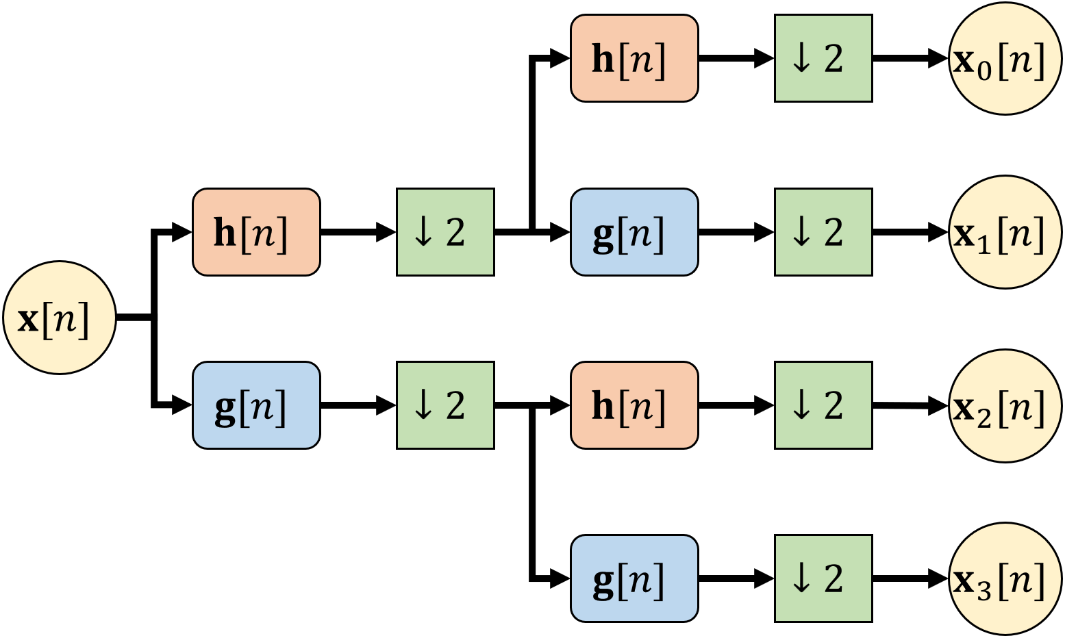
Figure 1: $N=4$ band ($M=2$ stage) subband decomposition filter bank structure for the orthogonal transform. The length of $\mathbf{x}$ is $N$. The length of each $\mathbf{x}_{i}$ is $\frac{N}{4}$ for $i=0,1,2,3$. $\mathbf{X}=\{\mathbf{x}_{0},\mathbf{x}_{1},\mathbf{x}_{2},\mathbf{x}_{3}\}$ is the $N$-length output of the orthogonal transform. In HT, $\mathbf{h}[n]=\{1,1\}$ and $\mathbf{g}[n]=\{-1,1\}$. In BWT using Bior 1.3 coefficients, $\mathbf{h}[n]=\{-0.125,0.125,1,1,0.125,-0.125\}$ and $g[n]=\{-1,1\}$ [38].

The HT and DCT can be implemented using butterfly operations described in Eq. (1) in [39] and the filterbank implementation of BWT is also fast [18]. Therefore, the complexity of each transform on a $N$-length vector is $O(N\log_{2}N)$. The 2-dimensional (2D) transform is obtained from the 1-dimensional (1D) transform in a separable manner for computational efficiency. Thus, the complexity of a 2D transform on an $N\times N$ image is $O(N^{2}\log_{2}N)$ [40]. Furthermore, using the hybrid quantum-classical approach [41], the 1D-HT and the 2D-HT can be implemented in $O(N)$ and $O(N^{2})$ time, respectively, as a quantum logic gate can be implemented efficiently in parallel.

The DCT convolution theorem Theorem 1 is related to the DFT convolution theorem:

Theorem 1 (DCT convolution theorem)

Let $N\in\mathbb{N}_{+}$, and $\mathbf{a},\mathbf{x}\in\mathbb{R}^{N}$. Then, $\mathbf{y}=\mathbf{a}*_{s}\mathbf{x}\Longleftrightarrow\mathbf{Y}[k]=\mathbf{A}[k]\mathbf{X}[k]$, where, $\mathbf{Y}=\mathcal{D}(\mathbf{y}),\mathbf{A}=\mathcal{D}(\mathbf{a}),\mathbf{X}=\mathcal{D}(\mathbf{x}).$

Where, $\mathcal{D}(\cdot)$ stands for DCT, $*_{s}$ stands for the symmetric convolution. The relation between the symmetric convolution $*_{s}$ and the linear convolution $*$ is given by

$$\mathbf{a}*_{s}\mathbf{x}=\mathbf{\tilde{a}}*\mathbf{x}$$ (6)

where $\mathbf{\tilde{a}}$ is the symmetrically extended kernel in $\mathbb{R}^{2N-1}$:

$$\mathbf{\tilde{a}}_{k}=\mathbf{a}_{|N-1-k|},$$ (7)

for $k=0,1,...,2N-2$. The proof of Theorem 1 is presented in Section III in [42].

Similarly, we have the HT convolution theorem 2:

Theorem 2 (HT convolution theorem)

Let $M\in\mathbb{N}$, $N=2^{M}$, and $\mathbf{a},\mathbf{x}\in\mathbb{R}^{N}$. Then $\mathbf{y}=\mathbf{a}*_{d}\mathbf{x}\Longleftrightarrow\mathbf{Y}[k]=\mathbf{A}[k]\mathbf{X}[k]$, where, $\mathbf{Y}=\mathcal{H}(\mathbf{y})$, $\mathbf{A}=\mathcal{H}(\mathbf{a})$, $\mathbf{X}=\mathcal{H}(\mathbf{x})$.

Where, $\mathcal{H}(\cdot)$ stands for HT, $*_{d}$ represents the dyadic convolution. Although the dyadic convolution $*_{d}$ is not the same as circular convolution, we can still use the HT for convolutional filtering in neural networks. This is because HT is also related to the block Haar wavelet packet transform [18] and each Hadamard coefficient approximately represents a frequency band. As a result, applying weights onto frequency bands and computing the IHT is an approximate way of frequency domain filtering similar to the Fourier transform-based convolutional filtering. The proof of Theorem 2 is presented in [43].

In brief, convolution theorems have the property that convolution in the time or space domain is equivalent to element-wise multiplication in the transform domain. This property inspires us to design the neural network layers to replace the Conv2D layers in a deep neural network.

II-B Transform-Based Perceptron Layers

Fig. 2 presents the structures of the proposed transform-based perceptron layers. We propose two types of perceptron layers for each transform. One is a single-channel layer as shown in Fig. 2a, and the other is a multi-channel layer as shown in Fig. 2b. The multi-channel layer contains multiple times parameters as the single-channel layer, but it can produce a higher accuracy according to our experiments. In the transform domain of each channel, a scaling layer performs the filtering operation by element-wise multiplication. Then a $1\times 1$ Conv2D layer performs channel-wise filtering. After this step, there is a trainable soft-thresholding layer denoising the data and acting as the nonlinearity. In the single-channel layer, a shortcut connection is implemented. In the multi-channel layer, the outputs of all channels are summed up. We do not implement the shortcut connection in the multi-channel layer because there are multiple channels replacing the shortcut and they effectively transmit the derivatives to earlier layers. The 2D transform and its inverse along the width and height convert the tensor between the space domain and the transform domain.

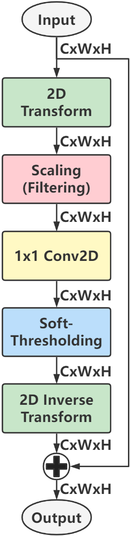
(a) 1-channel.

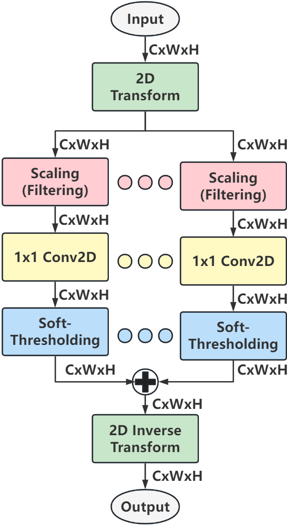
(b) Multi-channel.

Figure 2: (a) Single-channel perceptron layer and (b) multi-channel perceptron layer. Zero padding and truncation are applied in the HT-perceptron layers and the BWT-perceptron layers if the image size is not a power of 2.

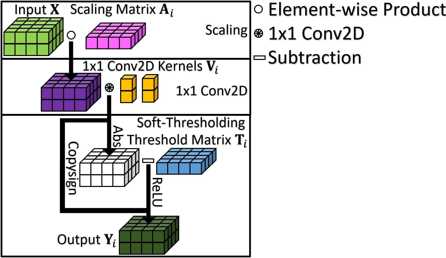
Figure 3: Processing in the transform domain.

The scaling layer is derived from Theorems 1 and 2, which state that the convolution in the space domain is equivalent to the element-wise multiplication in the transform domain. In detail, the input tensor in $\mathbb{R}^{C\times W\times H}$ is element-wise multiplied with a weight matrix in $\mathbb{R}^{W\times H}$ to perform an operation equivalent to the spatial domain convolutional filtering.

The trainable soft-thresholding layer is applied to remove small entries in the transform domain. It is similar to image coding and transform-domain denoising. It is defined as:

$$\mathbf{y}=\mathcal{S}_{T}(\mathbf{x})=\text{sign}(\mathbf{x})(|\mathbf{x}|-T)_{+},$$ (8)

where, $T$ is a non-negative trainable threshold parameter, $(\cdot)_{+}$ stands for the ReLU function. An input tensor in $\mathbb{R}^{C\times W\times H}$ is computed with threshold parameters in $\mathbb{R}^{W\times H}$, and these threshold parameters are determined using the back-propagation algorithm. The ReLU function is not suitable because both positive and negative values are important in the transform domain. A completely positive waveform can have both significant positive and negative values in the transform domain. Our ablation study on the CIFAR-10 dataset experimentally shows that the soft-thresholding function is superior to the ReLU function in the transform-based layers.

The overall process of each channel for the transform domain analysis (scaling, $1\times 1$ Conv2D, and soft-thresholding) is depicted in Figure 3. The single-channel and the $P$-channel transform-based perceptron layers are computed as:

$$\mathbf{y}=\mathcal{T}^{-1}\left(\mathcal{S}_{\mathbf{T}}\left(\mathcal{T}(\mathbf{x})\circ\mathbf{A}\circledast\mathbf{V}\right)\right)+\mathbf{x},$$ (9)

$$\mathbf{y}=\mathcal{T}^{-1}\left(\sum_{i=0}^{P-1}\mathcal{S}_{\mathbf{T}_{i}}\left(\mathcal{T}(\mathbf{x})\circ\mathbf{A}_{i}\circledast\mathbf{V}_{i}\right)\right),$$ (10)

where, $\mathcal{T}(\cdot)$ and $\mathcal{T}^{-1}(\cdot)$ stand for 2D transform (DCT, HT, or BWT) and 2D inverse transform, $\mathbf{A}$ and $\mathbf{A}_{i}$ are the scaling matrices, $\mathbf{V}$ and $\mathbf{V}_{i}$ are the kernels in the $1\times 1$ Conv2D layers, $\mathbf{T}$ and $\mathbf{T}_{i}$ are the threshold parameter matrices in the soft-thresholding, $\circ$ stands for the element-wise multiplication, and $\circledast$ represents the $1\times 1$ 2D convolution over an input composed of several input planes performed using PyTorch’s Conv2D API.

TABLE I: Parameters and Multiply–Accumulate (MACs) for a $C$-channel $N\times N$ tensor.

Layer (Operation)	Parameters	MACs
$K\times K$ Conv2D	$K^{2}C^{2}$	$K^{2}N^{2}C^{2}$
$3\times 3$ Conv2D	$9C^{2}$	$9N^{2}C^{2}$
2D-DCT/BWT/IDCT/IBWT (fast algorithm [18, 40])	$0$	$(\frac{5N^{2}}{2}\log_{2}N+\frac{N^{2}}{3}-6N+\frac{62}{3})C$
2D-DCT/BWT/IDCT/IBWT (matrix-vector product, used in this work.)	$0$	$2N^{3}C$
Scaling, Soft-Thresholding	$2N^{2}$	$N^{2}C$
$1\times 1$ Conv2D	$C^{2}$	$N^{2}C^{2}$
$P$-Channel DCT/BWT-Perceptron	$2PN^{2}+PC^{2}$	$4N^{3}C+PN^{2}C^{2}+PN^{2}C$
$P$-Channel HT-Perceptron	$2PN^{2}+PC^{2}$	$PN^{2}C^{2}+PN^{2}C$
Note: MACs from 2D-HT are omitted because there is no multiplication.

II-C Comparison with the Convolutional Layer

II-C1 Spatial and Channel Characteristics Comparison

The Conv2D layer has spatial-agnostic and channel-specific characteristics. Because of the spatial-agnostic characteristics of a Conv2D layer, the network cannot adapt different visual patterns corresponding to different spatial locations. On the contrary, the transform-based perceptron layer is location-specific and channel-specific. The 2D transform is location-specific but channel-agnostic, as it is computed using the entire block as a weighted summation on the spatial feature map. The scaling layer is also location-specific but channel-agnostic, as different scaling parameters (filters) are applied on different entries, and weights are shared in different channels. That is why we also use PyTorch’s $1\times 1$ Conv2D to make the transform-based perceptron layer channel-specific.

Figure 4 shows the comparison of the spatial and channel characteristics. Because the Conv2D layer is spatial-agnostic, the convolutional kernels cannot utilize the information from the location of the pixels. Conversely, the transform-based perceptron layer is location-specific, which means each weight parameter gains the location information.

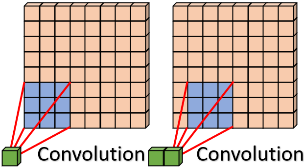
(a) Conv2D

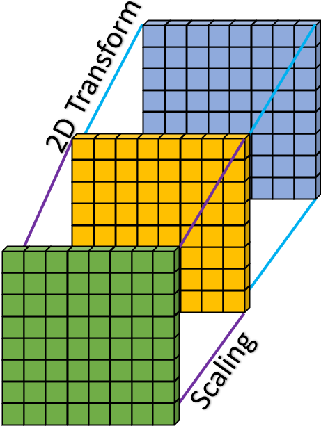
(b) Proposed layers

Figure 4: To compute different entries of an output slice, the Conv2D layer uses the same weights while the proposed transform-based perceptron layer uses different weights. Thus, the Conv2D layer is spatial-agnostic while the proposed transform-based perceptron layer is location-specific.

II-C2 Number of Parameters and MACs Comparison

The comparison of the number of parameters and Multiply–Accumulate (MACs) is presented in Table I. In a Conv2D layer, we need to compute $N^{2}K^{2}$ multiplications for a $C$-channel feature map of size $N\times N$ with a kernel size of $K\times K$. In the DCT-perceptron layer, there are $N^{2}$ multiplications from the scaling and $N^{2}$ multiplications from the $1\times 1$ Conv2D layer. There is no multiplication in the soft-thresholding function because the product between the sign of the input and the subtraction result can be implemented using the copysign operation. Although the 2D-DCT and the 2D-IDCT can be implemented in $O(N^{2}C\log_{2}N)$ using the fast algorithm [40], this fast approach is not officially supported in PyTorch. In this paper, we implement the 2D-DCT and the 2D-IDCT using the product between the DCT/IDCT weight matrix and the input tensor. Its complexity is $O(N^{3}C)$, and its MACs are $2N^{3}C$. Therefore, A $P$-channel DCT-perceptron layer has $2PN^{2}+PC^{2}$ parameters with $4N^{2}C+PN^{2}C^{2}+PN^{2}C$ MACs.

The BWT-perceptron layer has the same number of parameters and MACs as the DCT-perceptron layer. As for the HT-perceptron layers, because the HT is a multiple-free transform, there are only $2PN^{2}+PC^{2}$ parameters with $PN^{2}C+PN^{2}C^{2}$ MACs in the $P$-channel HT-perceptron layer. A 3-channel perceptron layer has the same amount of parameters but fewer MACs compared to a $3\times 3$ Conv2D layer if $C=N$. Therefore, in the experiment section, we mainly use the 3-channel perception layer to compare with the Conv2D layer. Furthermore, in most main-stream CNNs, $C$ is usually much larger than $N$ in the hidden layers, then our proposed perceptron layers can reduce parameters and computational cost for these CNNs even with the matrix-vector product for the transforms.

II-D Introduce Transform-based Perceptron Layers into ResNets

In this paper, we introduce the proposed layers into ResNet-18, ResNet-20, and ResNet-50. Fig. 5a shows the commonly used convolutional blocks in ResNets. The V1 version that contains two $3\times 3$ Conv2D layers are used in ResNet-18 and ResNet-20, and the V2 version that contains one $3\times 3$ and two one $1\times 1$ Conv2D layers is used in ResNet-50. As Fig. 5b shows, we replace the second $3\times 3$ Conv2D layer in each convolutional block V1, and the $3\times 3$ Conv2D layer in some convolutional blocks V2.

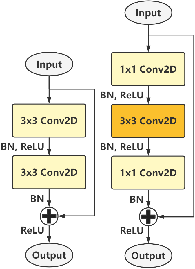
(a) ResNet Conv2D blocks.

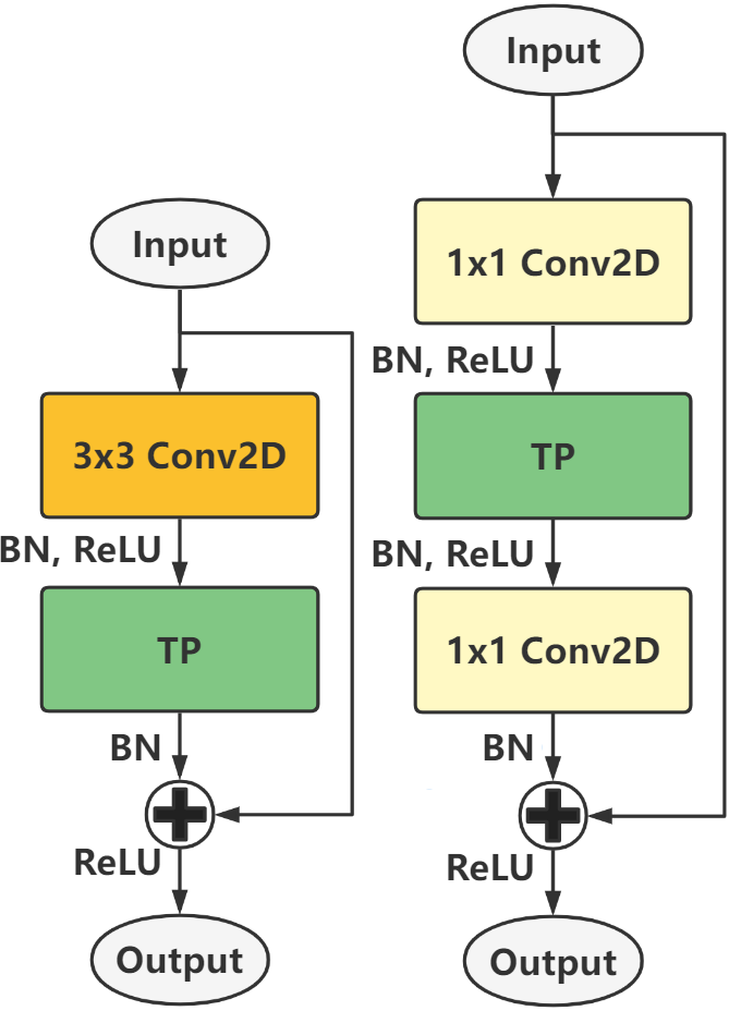
(b) ResNet TP blocks.

Figure 5: (a) ResNet’s convolutional residual blocks V1 (left) and V2 (right) versus (b) the proposed transform-based Perceptron (TP) residual blocks V1 (left) and V2 (right). BN stands for batch normalization. One $3\times 3$ Conv2D layer in each block is replaced by one proposed DCT-perceptron layer.

TABLE II: Structure of ResNet-20 with the transform-based perceptron (TP) layer for CIFAR-10 classification.

Layer	Output Shape	Implementation Details
Input	$3\times 32\times 32$	-
Conv1	$16\times 32\times 32$	$3\times 3,16$
Conv2_x	$16\times 32\times 32$	$\left[\begin{array}[]{c}3\times 3,16\\ \bf{\text{TP},16}\end{array}\right]\times 3$
Conv3_x	$32\times 16\times 16$	$\left[\begin{array}[]{c}3\times 3,32\\ \bf{\text{TP},32}\end{array}\right]\times 3$
Conv4_x	$64\times 8\times 8$	$\left[\begin{array}[]{c}3\times 3,32\\ \bf{\text{TP},64}\end{array}\right]\times 3$
GAP	$64$	Global Average Pooling
Output	$10$	Linear
Note: Building blocks are shown in brackets, with the numbers of blocks stacked. Downsampling with a stride of 2 is performed by Conv3_1 and Conv4_1.

TABLE III: Structure of ResNet-18 with the transform-based perceptron (TP) layers for ImageNet-1K classification.

Layer	Output Shape	Implementation Details
Input	$3\times 224\times 224$	-
Conv1	$64\times 112\times 112$	$7\times 7,64$, stride 2
MaxPool	$64\times 56\times 56$	$2\times 2$, stride 2
Conv2_x	$64\times 56\times 56$	$\left[\begin{array}[]{c}3\times 3,64\\ \bf{\text{TP},64}\end{array}\right]\times 2$
Conv3_x	$128\times 28\times 28$	$\left[\begin{array}[]{c}3\times 3,128\\ \bf{\text{TP},128}\end{array}\right]\times 2$
Conv4_x	$256\times 14\times 14$	$\left[\begin{array}[]{c}3\times 3,256\\ \bf{\text{TP},256}\end{array}\right]\times 2$
Conv5_x	$512\times 7\times 7$	$\left[\begin{array}[]{c}3\times 3,512\\ \bf{\text{TP},512}\end{array}\right]\times 2$
GAP	$512$	Global Average Pooling
Output	$1000$	Linear
Note: Building blocks are shown in brackets, with the numbers of blocks stacked. Downsampling with a stride of 2 is performed by Conv3_1, Conv4_1, and Conv5_1.

TABLE IV: Structure of ResNet-50 with the transform-based perceptron (TP) layers for ImageNet-1K classification.

Layer	Output Shape	Implementation Details
Input	$3\times 224\times 224$	-
Conv1	$64\times 112\times 112$	$7\times 7,64$, stride 2
MaxPool	$64\times 56\times 56$	$2\times 2$, stride 2
Conv2_1	$256\times 56\times 56$	$\left[\begin{array}[]{c}1\times 1,64\\ 3\times 3,64,\\ 1\times 1,256\end{array}\right]$
Conv2_2	$256\times 56\times 56$	$\left[\begin{array}[]{c}1\times 1,64\\ \bf{\text{TP},64}\\ 1\times 1,256\end{array}\right]$
Conv2_3	$256\times 56\times 56$	$\left[\begin{array}[]{c}1\times 1,64\\ 3\times 3,64\\ 1\times 1,256\end{array}\right]$
Conv3_1	$512\times 28\times 28$	$\left[\begin{array}[]{c}1\times 1,128\\ 3\times 3,128,\text{stride }2\\ 1\times 1,512\end{array}\right]$
Conv3_2	$512\times 28\times 28$	$\left[\begin{array}[]{c}1\times 1,128\\ \bf{\text{TP},128}\\ 1\times 1,512\end{array}\right]$
Conv3_3	$512\times 28\times 28$	$\left[\begin{array}[]{c}1\times 1,128\\ 3\times 3,128\\ 1\times 1,512\end{array}\right]$
Conv3_4	$512\times 28\times 28$	$\left[\begin{array}[]{c}1\times 1,128\\ \bf{\text{TP},128}\\ 1\times 1,512\end{array}\right]$
Conv4_1	$1024\times 14\times 14$	$\left[\begin{array}[]{c}1\times 1,256\\ 3\times 3,256,\text{stride }2\\ 1\times 1,1024\end{array}\right]$
Conv4_2	$1024\times 14\times 14$	$\left[\begin{array}[]{c}1\times 1,256\\ \bf{\text{TP},256}\\ 1\times 1,1024\end{array}\right]$
Conv4_3	$1024\times 14\times 14$	$\left[\begin{array}[]{c}1\times 1,256\\ 3\times 3,256\\ 1\times 1,1024\end{array}\right]$
Conv4_4	$1024\times 14\times 14$	$\left[\begin{array}[]{c}1\times 1,256\\ \bf{\text{TP},256}\\ 1\times 1,1024\end{array}\right]$
Conv4_5	$1024\times 14\times 14$	$\left[\begin{array}[]{c}1\times 1,256\\ 3\times 3,256\\ 1\times 1,1024\end{array}\right]$
Conv4_6	$1024\times 14\times 14$	$\left[\begin{array}[]{c}1\times 1,256\\ \bf{\text{TP},256}\\ 1\times 1,1024\end{array}\right]$
Conv5_1	$2048\times 7\times 7$	$\left[\begin{array}[]{c}1\times 1,512\\ 3\times 3,512,\text{stride }2\\ 1\times 1,2048\end{array}\right]$
Conv5_2	$2048\times 7\times 7$	$\left[\begin{array}[]{c}1\times 1,512\\ \bf{\text{TP},512}\\ 1\times 1,2048\end{array}\right]$
Conv5_3	$2048\times 7\times 7$	$\left[\begin{array}[]{c}1\times 1,512\\ 3\times 3,512\\ 1\times 1,2048\end{array}\right]$
GAP	$2048$	Global Average Pooling
Output	$1000$	Linear

To revise ResNet-20, ResNet-18, and ResNet-50, we retain the first $3\times 3$ Conv2D layer, then we replace those $3\times 3$ Conv2D layers at the even indices (the second Conv2D in each convolutional block in ResNet-20 and ResNet-18, and Conv2_2, Conv3_2, Conv3_4, etc., in ResNet-50) with the proposed transform-based perception layers. We keep the $3\times 3$ Conv2D layers at odd indices because, in this way, we use the regular $3\times 3$ Conv2D layer and the proposed HT-perceptron layer by turns, then the network can extract features in different manners efficiently. Table II describes the method we revising the ResNet-20 for the CIFAR-10 classification task, and Tables III and IV present the revised ResNet-18 and ResNet-50 for the ImageNet-1K classification task.

In the following sections, to call the revised ResNets, we add $P$C-Transform in front of their name. For example, 3C-DCT-ResNet-20 is the ResNet-20 revised by the three-channel DCT-perceptron layer. The BWT-ResNets are implemented using Bior 1.3 coefficients [38].

III Experimental Results

Our experiments are carried out on a workstation computer with an NVIDIA RTX 3090 GPU. The code is written in PyTorch in Python 3. The experiments include the CIFAR-10 classification task and the ImageNet-1K classification task. In the CIFAR-10 experiments, ResNet-20 is used as the backbone network. In the ImageNet-1K experiments, ResNet-18 and ResNet-50 are used as the backbone networks. The CIFAR-10 experiments carry out our ablation study. Fig. 6 presents the test error history of our models.

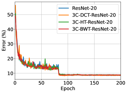
(a) CIFAR-10

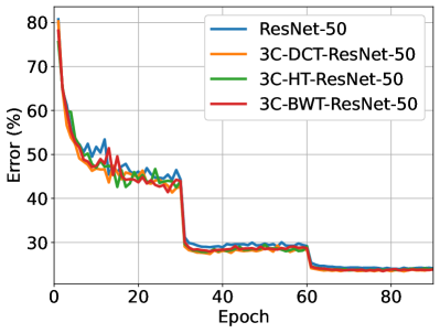
(b) ImageNet-1K (224²)

Figure 6: Training on CIFAR-10 and ImageNet-1K. In (a), curves denote test error. Comparable CIFAR-10 accuracy results are obtained using the proposed tri-channel HT/DCT-perceptron layers, while more than 26% parameters and 14% MACs are reduced. In (b), curves denote the validation error of the center crops. The models are revised under the revision 2 structure. Better ImageNet-1K accuracy results are obtained using the proposed tri-channel HT/DCT-perceptron layers, while more than 11% parameters and 11% MACs are reduced.

III-A CIFAR-10 Experiments

Training ResNet-20 and its revisions follow the implementation in [1]. In detail, we use an SGD optimizer with a weight decay of 0.0001 and momentum of 0.9. Models are trained with a mini-batch size of 128 for 200 epochs. The initial learning rate is 0.1, and the learning rate is reduced by a factor of 1/10 at epochs 82, 122, and 163, respectively. Data augmentation is implemented as follows: First, we pad 4 pixels on the training images. Then, we apply random cropping to get 32 by 32 images. Finally, we randomly flip images horizontally. We normalize the images with the means of [0.4914, 0.4822, 0.4465] and the standard variations of [0.2023, 0.1994, 02010]. During the training, the best models are saved based on the accuracy of the CIFAR-10 test dataset, and their accuracy numbers are reported in Table V.

TABLE V: CIFAR-10 Experimental Results.

Method	Parameters	MACs (M)	Accuracy
ResNet-20 [1] (official)	0.27M	-	91.25%
HT-based ResNet-20 [29]	133,082 (51.16%$\downarrow$)	-	90.12%
ResNet-20 (our trial, baseline)	272,474	41.32	91.66%
1C-DCT-ResNet-20	151,514 (44.39%$\downarrow$)	30.79 (25.5%$\downarrow$)	91.59%
3C-DCT-ResNet-20	199,898 (26.64%$\downarrow$)	35.68 (13.6%$\downarrow$)	91.75%
1C-HT-ResNet-20	151,514 (44.39%$\downarrow$)	22.53 (45.5%$\downarrow$)	91.25%
3C-HT-ResNet-20	199,898 (26.64%$\downarrow$)	27.42 (33.6%$\downarrow$)	91.29%
3C-BWT-ResNet-20	199,898 (26.64%$\downarrow$)	35.68 (13.6%$\downarrow$)	91.35%
ResNet-20+1C-DCT-P.	276,826 (1.60%$\uparrow$)	41.65 (0.8%$\uparrow$)	91.82%

As Table V shows, on the one hand, DCT-ResNet-20, which is implemented by revising Conv2D layers using the single-channel DCT-perceptron layers, contains 44.39% fewer parameters than the baseline ResNet-20 model, but it only suffers a 0.07% accuracy lost. On the other hand, the 3C-DCT-ResNet-20, which is implemented using the tri-channel DCT-perceptron layers, contains 22.64% fewer parameters than the baseline ResNet-20 model, but it even reaches a 0.09% higher accuracy. The 1C-HT-ResNet-20 and the 3C-HT-ResNet-20 have the same parameter savings (44.39% and 26.64%) as the 1C-DCT-ResNet-20 and the 3C-DCT-ResNet-20, and their accuracy losses are both less than 0.6% compared to the baseline model. The reason that the HT models get lower accuracy results than the corresponding DCT models is that HT is a binary transform, which means its ability for frequency information extraction is weaker than the DCT. As compensation, fewer computational cost is required to compute those HT models. Figure 6a shows the test error history of the ResNet-20, the 3C-HT-ResNet-20, and the 3C-DCT-ResNet-20 on the CIFAR-10 test dataset.

Compare to our previous HT-based work in [29] which is also single-channel, the proposed 1C-HT-ResNet-20 reaches a 1.03% higher accuracy. This is because the HT layer in [29] is channel-agnostic, while the proposed layer is channel-specific. Therefore, the proposed layers can utilize channel-wise information.

Another application for the proposed layers is that we can insert one additional layer before the global average pooling layer in the ResNets (the location is after the output of the final convolutional block). For example, an extra DCT-perceptron layer improves the accuracy of the regular ResNet-20 to 91.82%. This method is named ResNet-20+1C-DCT-P.

TABLE VI: CIFAR-10 ablation study.

Method	Parameters	Accuracy
ResNet-20 (our trial, baseline)	272,474	91.66%
1C-DCT-ResNet-20	151,514 (44.39%$\downarrow$)	91.59%
(without shortcut in 1C-DCT-P.)	151,514 (44.39%$\downarrow$)	91.12%
(without scaling in 1C-DCT-P.)	147,482 (45.87%$\downarrow$)	90.46%
(ReLU with thresholds in 1C-DCT-P.)	151,514 (44.39%$\downarrow$)	91.30%
(ReLU w/o thresholds in 1C-DCT-P.)	147,818 (45.75%$\downarrow$)	91.06%
(replacing all Conv2D)	51,034 (81.31%$\downarrow$)	85.74%
2C-DCT-ResNet-20	175,706 (35.51%$\downarrow$)	91.42%
3C-DCT-ResNet-20	199,898 (26.64%$\downarrow$)	91.75%
(with shortcut in 3C-DCT-P.)	199,898 (26.64%$\downarrow$)	91.50%
4C-DCT-ResNet-20	224,090 (17.76%$\downarrow$)	91.48%
5C-DCT-ResNet-20	248,282 (8.88%$\downarrow$)	91.47%
2C-HT-ResNet-20	175,706 (35.51%$\downarrow$)	91.28%
3C-HT-ResNet-20	199,898 (26.64%$\downarrow$)	91.29%
4C-HT-ResNet-20	224,090 (17.76%$\downarrow$)	91.50%
5C-HT-ResNet-20	248,282 (8.88%$\downarrow$)	91.58%
6C-HT-ResNet-20	272,474 (0.00%$\downarrow$)	91.21%
Note: DCT-P. stands for the DCT-perceptron layer.

Table VI presents our ablation study on the CIFAR-10 dataset. First, we remove the residual design (the shortcut connection) in the single-channel DCT-perceptron layers and we obtain a worse accuracy (91.12%). Therefore, the shortcut connection can improve the performance of the single-channel DCT-perceptron layer. Then, we remove scaling which is the convolutional filtering in the single-channel DCT-perceptron layers. In this case, the multiplication operations in the single-channel DCT-perceptron layer are only implemented in the $1\times 1$ Conv2D. The accuracy drops from 91.59% to 90.46%. Therefore, scaling is necessary to maintain accuracy, as it makes use of the convolution theorems. Next, we apply ReLU instead of soft-thresholding in the single-channel DCT-perceptron layers. We first apply the same thresholds as the soft-thresholding thresholds on ReLU. In this case, the number of parameters is the same as in the proposed 1C-DCT-ResNet-20 model, but the accuracy drops to 91.30%. We then try regular ReLU with a bias term in the $1\times 1$ Conv2D layers in the single-channel DCT-perceptron layers, and the accuracy drops further to 91.06%. These experiments show that the soft-thresholding is superior to the ReLU in this work, as the soft-thresholding retains negative frequency components with high amplitudes, which are also used in denoising and image coding applications. Furthermore, we replace all Conv2D layers in the ResNet-20 model with the single-channel DCT-perceptron layers. We implement the downsampling (Conv2D with the stride of 2) by truncating the IDCT2D so that each dimension of the reconstructed image is one-half the length of the original. In this method, 81.31% parameters are reduced, but the accuracy drops to 85.74% due to lacking parameters.

In the ablation study on the multi-channel DCT-perceptron layer, we further try the structures with 2/4/5 channels, but their accuracy results are all lower than the tri-channel. A similar ablation study is taken on the HT-perceptron layer, and the best accuracy result is obtained using 5 channels. Normally, the more channels the layer has, the better performance it can reach because of the more parameters. However, too many channels may cause redundancy and make it hard to train the layer well using the back-propagation algorithm.

Furthermore, we add the shortcut connection in the tri-channel DCT-perception layer, but our experiments show that the shortcut connection is redundant in the tri-channel DCT-perception layer. This may be because three channels are replacing the shortcut. The multi-channel structure allows the derivatives to propagate to earlier channels better than the single-channeled structure.

TABLE VII: ImageNet-1K results. Center-crop top-1 accuracy is used for evaluation. The image size is $224\times 224$.

Method	Publication	Parameters (M)	MACs (G)	Center-Crop Accuracy		10-Crop Accuracy
				Top-1	Top-5	Top-1	Top-5
ResNet-18 [1] (Torchvision [44], baseline)	CVPR 2015	11.69	1.82	69.76%	89.08%	71.86%	90.60%
DCT-based ResNet-18 [24]	IJCNN 2021	8.74	-	68.31%	88.22%	-	-
1C-DCT-ResNet-18	This Paper	6.14 (47.5%$\downarrow$)	1.47 (19.3%$\downarrow$)	67.84%	87.73%	70.09%	89.40%
3C-DCT-ResNet-18	This Paper	7.56 (35.3%$\downarrow$)	1.57 (13.6%$\downarrow$)	69.55%	89.04%	71.91%	90.55%
3C-DCT-ResNet-18+1C-DCT-P.	This Paper	7.82 (33.1%$\downarrow$)	1.59 (12.8%$\downarrow$)	70.00%	89.07%	72.33%	90.54%
ResNet-50 [1] (Torchvision [44])	CVPR 2015	25.56	4.12	76.13%	92.86%	77.43%	93.75%
Order 1 + ScatResNet-50 [31]	ECCV 2018	27.8	-	74.5%	92.0%	-	-
JPEG-ResNet-50 [21]	NIPS 2018	28.4	5.4	76.06%	93.02%	-	-
ResNet-50+DCT+FBS (3x32) [22]	ICIP 2020	26.2	3.68	70.22%	-	-	-
ResNet-50+DCT+FBS (3x16) [22]	ICIP 2020	25.6	3.18	67.03%	-	-	-
FFC-ResNet-50 (+LFU, $\alpha=0.25$) [19]	NIPS 2020	26.7	4.3	77.8%	-	-	-
FFC-ResNet-50 ($\alpha=1$) [19]	NIPS 2020	34.2	5.6	75.2%	-	-	-
Faster JPEG-ResNet-50 [23]	CIARP 2021	25.1	2.86	70.49%	-	-	-
DCT-based ResNet-50 [24]	IJCNN 2021	21.30	-	74.73%	92.30%	-	-
Harm-DCT-ResNet-50 [25]	PR 2022	25.6	-	77.02%	93.36%	-	-
Harm-DCT-ResNet-50, progr.$\lambda$ [25]	PR 2022	19.7	-	76.79%	93.33%
ResNet-50 (AugSkip) ZerO Init [26]	ICLR 2022	25.56	4.12	76.37%	-	-	-
ResNet-50 (our trial, baseline)	-	25.56	4.12	76.06%	92.85%	77.53%	93.75%
3C-DCT-ResNet-50	This Paper	22.62 (11.5%$\downarrow$)	3.63 (12.0%$\downarrow$)	76.56%	93.15%	78.04%	94.05%
3C-HT-ResNet-50	This Paper	22.63 (11.5%$\downarrow$)	3.60 (12.6%$\downarrow$)	76.36%	93.02%	77.79%	94.02%
3C-BWT-ResNet-50	This Paper	22.63 (11.5%$\downarrow$)	3.75 (9.0%$\downarrow$)	76.53%	93.13%	77.98%	94.11%
ResNet-50 (our trial, baseline, input $256^{2}$)	-	25.56	5.38	76.18%	92.94%	77.61%	93.88%
3C-DCT-ResNet-50 (input $256^{2}$)	This Paper	22.63 (11.5%$\downarrow$)	4.76 (11.5%$\downarrow$)	77.00%	93.52%	78.62%	94.36%
3C-HT-ResNet-50 (input $256^{2}$)	This Paper	22.63 (11.5%$\downarrow$)	4.58 (14.9%$\downarrow$)	76.77%	93.26%	78.33%	94.14%
3C-BWT-ResNet-50 (input $256^{2}$)	This Paper	22.63 (11.5%$\downarrow$)	4.76 (11.5%$\downarrow$)	77.07%	93.43%	78.45%	94.34%
Note: MACs of DCT/BWT in this work are computed using the matrix-vector product. These numbers can be reduced further if the transforms are implemented using the Cooley–Tukey algorithm [40]. MACs of the FFT in [19] are omitted by its authors. Models in [25] were trained with 100 epochs instead of 90.

TABLE VIII: ImageNet-1K results of inserting an additional DCT-perceptron layer. The image size is $224\times 224$.

Method	Parameters (M)	MACs (G)	Center-Crop Accuracy		10-Crop Accuracy
			Top-1	Top-5	Top-1	Top-5
ResNet-18	11.69	1.82	69.76%	89.08%	71.86%	90.60%
ResNet-18+1C-DCT-P.	11.95 (2.3%$\uparrow$)	1.84 (0.3%$\uparrow$)	70.50%	89.29%	72.89%	90.98%
ResNet-50	25.56	4.12	76.06%	92.85%	77.53%	93.75%
ResNet-50+1C-DCT-P.	29.76 (16.4%$\uparrow$)	4.33 (5.1%$\uparrow$)	76.09%	93.80%	77.67%	93.84%

III-B ImageNet-1K Classification

In this section, we employ PyTorch’s official ImageNet-1K training code [45]. Because we use the PyTorch official training code with the default training configuration for the revised ResNet-18s training, we use PyTorch Torchvision’s officially trained ResNet-18 model as the baseline. On the other hand, the default training for ResNet-50 requires about 26–30 GB GPU memory, while an NVIDIA RTX3090 GPU only has 24GB. To overcome the issue of memory deficiency, we halve the batch size and the learning rate correspondingly. We use an SGD optimizer with a weight decay of 0.0001 and momentum of 0.9 for 90 epochs. Revised ResNet-18’s are trained with the default setting: a mini-batch size of 256, and an initial learning rate of 0.1. ResNet-50 and its revised models are trained with a mini-batch size of 128, the initial learning rate is 0.05. The learning rate is reduced by a factor of 1/10 after every 30 epochs. For data argumentation, we apply random resized crops on training images to get 224 by 224 images, then we randomly flip images horizontally. In testing on the ImageNet-1K validation dataset, we resize the images to make the smaller edge of images 256, then apply center crops on the resized testing images to get 224 by 224 images. We normalize the images with the means of [0.485, 0.456, 0.406] and the standard variations of [0.229, 0.224, 0.225], respectively. We evaluate our models on the ImageNet-1K validation dataset and compare them with the state-of-art papers. During the training, the best models are saved based on the center-crop top-1 accuracy on the ImageNet-1K validation dataset, and their accuracy numbers are presented in Table VII. Furthermore, we carry out experiments with the input size of 256 by 256, for 256 is the smallest integer power of 2 which is larger than 224. The training strategies except for the image size are the same as the experiments with the image size of 224 by 224. We resize the validation images to make the smaller edge 292, then apply center crops on the resized testing images to get 256 by 256 images. In Table VII, the input sizes in the last 4 rows are $256\times 256$, and in other rows are $224\times 224$. Fig. 6b shows the test error history of the ResNet-50 and our revised ResNet-50s on the ImageNet-1K validation dataset.

When the input size is 224 by 224, the 3C-HT-ResNet-50 and the 3C-BWT-ResNet-50 have more parameters and more MACs than the 3C-DCT-ResNet-50. This is because the input size is not a pair of integers power of 2, so the hidden tensors’ sizes in the HT-perceptron layer and the BWT-perceptron layer are larger than in the DCT-perceptron layer. Although the HT is still more efficient than the DCT, the scaling, $1\times 1$ Conv2D, and soft-thresholding in the HT-perceptron layers need to be computed with tensors with larger sizes. Furthermore, if the input size satisfies the constraint of integers power of 2, the 3C-HT-ResNet-50 takes less computational cost than the 3C-DCT-ResNet-50, and the 3C-BWT-ResNet-50 takes the same computational cost as the 3C-DCT-ResNet-50. As Table VII presents, all transform-based perceptron layers manage to improve the accuracy for ResNet-50 by reducing the number of parameters and the MACs. For example, the 3C-BWT-ResNet layer improves the center-crop top-1 accuracy of ResNet-50 from 76.18% to 77.07%, while 11.5% parameters and MACs are reduced.

Other state-of-art transform-based methods are listed in Table VII for comparison. In FFC-ResNet-50 (+LFU, $\alpha=0.25$) [19], authors use their proposed Fourier Units (FU) and local Fourier units (LFU) to process only 25% channels of each input tensor and use the regular $3\times 3$ Conv2D to process the remaining to get the accuracy of 77.8%. Although this method improves the accuracy, it also increases the number of parameters and MACs. We can also use a combination of regular the $3\times 3$ Conv2D layers and our proposed layers to increase the accuracy by increasing the parameters in their method. However, according to the ablation study in [19], if all channels are processed by their proposed FU, FFC-ResNet-50 ($\alpha=1$) only gets the accuracy of 75.2%. The reported number of parameters and MACs are much higher than the baseline in [19] even though MACs from the FFT and IFFT are not counted. Our methods improve accuracy for regular ResNet-50s with significantly reduced parameters and MACs. Models in [25] were trained with 10 additional epochs. Our results can also be improved with further training. Pruning-based methods [46, 47] can be implemented as a part of our method to prune some layers because we implement convolutions in the transform domain. For example, removing convolutional filtering is equivalent to removing the corresponding DCT, scaling, soft-thresholding, and inverse DCT operation.

The experiments of inserting one additional layer before the global average pooling layer in the ResNet-18 and the ResNet-50 are presented in Table VIII. The additional single-channel DCT-perceptron layer improves the accuracy of ResNet-18 and ResNet-50 respectively with negligible extra parameters and computational cost.

III-C Wall-Clock Time

Although in this work, we do not apply any CUDA-based coding to accelerate the proposed layers, it is worthy to present the wall-clock time of the models. Specially, we find a CUDA implementation for HT at [48, 49], so we implement HT using it in this section. DCT and BWT are still implemented as a matrix-vector product without taking advantage of the fast ($O(N^{2}\log_{2}N)$) algorithm [18, 40] because PyTorch does not support DCT and the wavelet transforms at the moment. Scaling and Soft-thresholding are also implemented using pure PyTorch.

Since we use the matrix-vector product to implement DCT and BWT, the time consumption of each transform is the same if the padding is not needed (i.e., the input size is $32^{2}$ or $256^{2}$). The speed test is performed on the NVIDIA RTX3090 GPU using the batch size of 1. The CPU of the computer is Intel(R) Xeon(R) W-2255 CPU @ 3.70GHz. We first warm up the device by 10 inference times, then compute the average inference time of 100 inferences. The wall-clock time is presented in Table IX. Even without any CUDA-based optimization, our transform-based ResNet models take less than $3\times$ time that of the regular ResNet models which are well-optimized using CUDA. The time differences are small as shown in Table IX. Furthermore, we calculate the transforms of the entire tensor in the current work, but we can calculate them using smaller blocks such as $8\times 8$ blocks as in JPEG and MPEG video coding methods to reduce memory usage and latency.

TABLE IX: Wall-Clock Time.

Method	Input Size	Time (mS)
ResNet-20	$3\times 32\times 32$	4.9
1C-HT-ResNet-20	$3\times 32\times 32$	6.7
1C-DCT-ResNet-20	$3\times 32\times 32$	10.4
1C-BWT-ResNet-20	$3\times 32\times 32$	10.4
3C-HT-ResNet-20	$3\times 32\times 32$	10.1
3C-DCT-ResNet-20	$3\times 32\times 32$	13.7
3C-BWT-ResNet-20	$3\times 32\times 32$	13.7
ResNet-50	$3\times 224\times 224$	12.0
1C-HT-ResNet-50	$3\times 224\times 224$	14.4
1C-DCT-ResNet-50	$3\times 224\times 224$	17.2
1C-BWT-ResNet-50	$3\times 224\times 224$	17.3
3C-HT-ResNet-50	$3\times 224\times 224$	17.5
3C-DCT-ResNet-50	$3\times 224\times 224$	20.1
3C-BWT-ResNet-50	$3\times 224\times 224$	20.2
ResNet-50	$3\times 256\times 256$	12.6
1C-HT-ResNet-50	$3\times 256\times 256$	14.5
1C-DCT-ResNet-50	$3\times 256\times 256$	17.4
1C-BWT-ResNet-50	$3\times 256\times 256$	17.4
3C-HT-ResNet-50	$3\times 256\times 256$	17.5
3C-DCT-ResNet-50	$3\times 256\times 256$	20.3
3C-BWT-ResNet-50	$3\times 256\times 256$	20.3

IV Conclusion

In this paper, we proposed a set of novel layers based on the discrete cosine transform (DCT), the Hadamard transform (HT), and the biorthogonal wavelet transform (BWT) to replace some of the $3\times 3$ Conv2D layers in convolutional neural networks (CNNs). All of our transform domain layers can be implemented with single-channel and multi-channel structures. The idea of this work is derived from the convolution theorems, that the convolution in the time and the space domain is equivalent to the element-wise multiplication in the transform domain. With the proposed layers, CNNs such as ResNets can obtain comparable or even higher accuracy results in image classification tasks with much fewer parameters. ResNets with the HT-perceptron layers usually produce a little lower accuracy than ResNets with the DCT-perceptron layers. This is because as a binary transform, the ability for frequency analysis of the HT is inferior to the DCT. As compensation, there is no multiplication to implement HT, while multiplications between the tensors and the DCT weights are required in DCT. Another application for the proposed layers is the addition of an extra layer to the regular ResNets. An additional transform domain layer before the global average pooling layer improves the accuracy of ResNets with a negligible increase in the number of parameters and computational time. In addition to ResNets, the proposed transform domain layers can be used in any convolutional neural network using the Conv2D layers.

References

- [1] K. He, X. Zhang, S. Ren, and J. Sun, “Deep residual learning for image recognition,” in Proceedings of the IEEE conference on computer vision and pattern recognition, 2016, pp. 770–778.
- [2] D. Badawi, H. Pan, S. C. Cetin, and A. E. Çetin, “Computationally efficient spatio-temporal dynamic texture recognition for volatile organic compound (voc) leakage detection in industrial plants,” IEEE Journal of Selected Topics in Signal Processing, vol. 14, no. 4, pp. 676–687, 2020.
- [3] C. Agarwal, S. Khobahi, D. Schonfeld, and M. Soltanalian, “Coronet: a deep network architecture for enhanced identification of covid-19 from chest x-ray images,” in Medical Imaging 2021: Computer-Aided Diagnosis, vol. 11597. International Society for Optics and Photonics, 2021, p. 1159722.
- [4] J. Redmon, S. Divvala, R. Girshick, and A. Farhadi, “You only look once: Unified, real-time object detection,” in Proceedings of the IEEE conference on computer vision and pattern recognition, 2016, pp. 779–788.
- [5] S. Aslan, U. Güdükbay, B. U. Töreyin, and A. E. Çetin, “Deep convolutional generative adversarial networks for flame detection in video,” in International Conference on Computational Collective Intelligence. Springer, 2020, pp. 807–815.
- [6] G. Menchetti, Z. Chen, D. J. Wilkie, R. Ansari, Y. Yardimci, and A. E. Çetin, “Pain detection from facial videos using two-stage deep learning,” in 2019 IEEE Global Conference on Signal and Information Processing (GlobalSIP). IEEE, 2019, pp. 1–5.
- [7] S. Aslan, U. Güdükbay, B. U. Töreyin, and A. E. Çetin, “Early wildfire smoke detection based on motion-based geometric image transformation and deep convolutional generative adversarial networks,” in ICASSP 2019-2019 IEEE International Conference on Acoustics, Speech and Signal Processing (ICASSP). IEEE, 2019, pp. 8315–8319.
- [8] M. S. Beratoğlu and B. U. Töreyin, “Vehicle license plate detector in compressed domain,” IEEE Access, vol. 9, pp. 95 087–95 096, 2021.
- [9] C. Yu, J. Wang, C. Peng, C. Gao, G. Yu, and N. Sang, “Bisenet: Bilateral segmentation network for real-time semantic segmentation,” in Proceedings of the European conference on computer vision (ECCV), 2018, pp. 325–341.
- [10] Z. Huang, X. Wang, L. Huang, C. Huang, Y. Wei, and W. Liu, “Ccnet: Criss-cross attention for semantic segmentation,” in Proceedings of the IEEE/CVF International Conference on Computer Vision, 2019, pp. 603–612.
- [11] J. Long, E. Shelhamer, and T. Darrell, “Fully convolutional networks for semantic segmentation,” in Proceedings of the IEEE conference on computer vision and pattern recognition, 2015, pp. 3431–3440.
- [12] R. P. Poudel, S. Liwicki, and R. Cipolla, “Fast-scnn: fast semantic segmentation network,” arXiv preprint arXiv:1902.04502, 2019.
- [13] Y. Jin, W. Hao, P. Wang, and J. Wang, “Fast detection of traffic congestion from ultra-low frame rate image based on semantic segmentation,” in 2019 14th IEEE Conference on Industrial Electronics and Applications (ICIEA). IEEE, 2019, pp. 528–532.
- [14] X. Dong, L. Qian, and L. Huang, “Short-term load forecasting in smart grid: A combined cnn and k-means clustering approach,” in 2017 IEEE international conference on big data and smart computing (BigComp). IEEE, 2017, pp. 119–125.
- [15] E. Koyuncu, “Centroidal clustering of noisy observations by using th power distortion measures,” IEEE Transactions on Neural Networks and Learning Systems, 2022.
- [16] R. Miao and E. Koyuncu, “Federated momentum contrastive clustering,” arXiv preprint arXiv:2206.05093, 2022.
- [17] R. V. Hartley, “A more symmetrical fourier analysis applied to transmission problems,” Proceedings of the IRE, vol. 30, no. 3, pp. 144–150, 1942.
- [18] A. E. Cetin, O. N. Gerek, and S. Ulukus, “Block wavelet transforms for image coding,” IEEE Transactions on Circuits and Systems for Video Technology, vol. 3, no. 6, pp. 433–435, 1993.
- [19] L. Chi, B. Jiang, and Y. Mu, “Fast fourier convolution,” Advances in Neural Information Processing Systems, vol. 33, pp. 4479–4488, 2020.
- [20] U. F. Mohammad and M. Almekkawy, “A substitution of convolutional layers by fft layers-a low computational cost version,” in 2021 IEEE International Ultrasonics Symposium (IUS). IEEE, 2021, pp. 1–3.
- [21] L. Gueguen, A. Sergeev, B. Kadlec, R. Liu, and J. Yosinski, “Faster neural networks straight from jpeg,” Advances in Neural Information Processing Systems, vol. 31, 2018.
- [22] S. F. dos Santos, N. Sebe, and J. Almeida, “The good, the bad, and the ugly: Neural networks straight from jpeg,” in 2020 IEEE International Conference on Image Processing (ICIP). IEEE, 2020, pp. 1896–1900.
- [23] S. F. dos Santos and J. Almeida, “Less is more: Accelerating faster neural networks straight from jpeg,” in Iberoamerican Congress on Pattern Recognition. Springer, 2021, pp. 237–247.
- [24] Y. Xu and H. Nakayama, “Dct-based fast spectral convolution for deep convolutional neural networks,” in 2021 International Joint Conference on Neural Networks (IJCNN). IEEE, 2021, pp. 1–8.
- [25] M. Ulicny, V. A. Krylov, and R. Dahyot, “Harmonic convolutional networks based on discrete cosine transform,” Pattern Recognition, vol. 129, p. 108707, 2022.
- [26] J. Zhao, F. Schäfer, and A. Anandkumar, “Zero initialization: Initializing residual networks with only zeros and ones,” arXiv, 2021.
- [27] T. C. Deveci, S. Cakir, and A. E. Cetin, “Energy efficient hadamard neural networks,” arXiv preprint arXiv:1805.05421, 2018.
- [28] H. Pan, D. Badawi, and A. E. Cetin, “Fast walsh-hadamard transform and smooth-thresholding based binary layers in deep neural networks,” in Proceedings of the IEEE/CVF Conference on Computer Vision and Pattern Recognition, 2021, pp. 4650–4659.
- [29] ——, “Block walsh–hadamard transform-based binary layers in deep neural networks,” ACM Transactions on Embedded Computing Systems, vol. 21, no. 6, pp. 1–25, 2022.
- [30] P. Liu, H. Zhang, W. Lian, and W. Zuo, “Multi-level wavelet convolutional neural networks,” IEEE Access, vol. 7, pp. 74 973–74 985, 2019.
- [31] E. Oyallon, E. Belilovsky, S. Zagoruyko, and M. Valko, “Compressing the input for cnns with the first-order scattering transform,” in Proceedings of the European Conference on Computer Vision (ECCV), 2018, pp. 301–316.
- [32] D. L. Donoho, “De-noising by soft-thresholding,” IEEE transactions on information theory, vol. 41, no. 3, pp. 613–627, 1995.
- [33] O. Karakuş, I. Rizaev, and A. Achim, “A simulation study to evaluate the performance of the cauchy proximal operator in despeckling sar images of the sea surface,” in IGARSS 2020-2020 IEEE International Geoscience and Remote Sensing Symposium. IEEE, 2020, pp. 1568–1571.
- [34] D. Badawi, A. Agambayev, S. Ozev, and A. E. Cetin, “Discrete cosine transform based causal convolutional neural network for drift compensation in chemical sensors,” in ICASSP 2021-2021 IEEE International Conference on Acoustics, Speech and Signal Processing (ICASSP). IEEE, 2021, pp. 8012–8016.
- [35] H. Pan, D. Badawi, C. Chen, A. Watts, E. Koyuncu, and A. E. Cetin, “Deep neural network with walsh-hadamard transform layer for ember detection during a wildfire,” in Proceedings of the IEEE/CVF Conference on Computer Vision and Pattern Recognition, 2022, pp. 257–266.
- [36] N. Ahmed, T. Natarajan, and K. R. Rao, “Discrete cosine transform,” IEEE transactions on Computers, vol. 100, no. 1, pp. 90–93, 1974.
- [37] G. Strang, “The discrete cosine transform,” SIAM review, vol. 41, no. 1, pp. 135–147, 1999.
- [38] P. Singh, P. Singh, and R. K. Sharma, “Jpeg image compression based on biorthogonal, coiflets and daubechies wavelet families,” International Journal of Computer Applications, vol. 13, no. 1, pp. 1–7, 2011.
- [39] B. J. Fino and V. R. Algazi, “Unified matrix treatment of the fast walsh-hadamard transform,” IEEE Transactions on Computers, vol. 25, no. 11, pp. 1142–1146, 1976.
- [40] M. Vetterli, “Fast 2-d discrete cosine transform,” in ICASSP’85. IEEE International Conference on Acoustics, Speech, and Signal Processing, vol. 10. IEEE, 1985, pp. 1538–1541.
- [41] A. Shukla and P. Vedula, “A hybrid classical-quantum algorithm for solution of nonlinear ordinary differential equations,” Applied Mathematics and Computation, p. 127708, 2022.
- [42] B. Shen, I. K. Sethi, and V. Bhaskaran, “Dct convolution and its application in compressed domain,” IEEE transactions on circuits and systems for video technology, vol. 8, no. 8, pp. 947–952, 1998.
- [43] A. Usakova, J. Kotuliaková, and M. ZAJAC, “Walsh–hadamard transformation of a convolution,” Radioengineering, vol. 11, no. 3, pp. 40–42, 2002.
- [44] “Models and pre-trained weights,” https://pytorch.org/vision/stable/models.html, 2022, accessed: 2022-09-27.
- [45] “Imagenet training in pytorch,” https://github.com/pytorch/examples/tree/main/imagenet, 2022, accessed: 2022-09-27.
- [46] H. Li, A. Kadav, I. Durdanovic, H. Samet, and H. P. Graf, “Pruning filters for efficient convnets,” arXiv preprint arXiv:1608.08710, 2016.
- [47] P. Molchanov, A. Mallya, S. Tyree, I. Frosio, and J. Kautz, “Importance estimation for neural network pruning,” in Proceedings of the IEEE/CVF conference on computer vision and pattern recognition, 2019, pp. 11 264–11 272.
- [48] A. Thomas, A. Gu, T. Dao, A. Rudra, and C. Ré, “Learning compressed transforms with low displacement rank,” Advances in neural information processing systems, vol. 31, 2018.
- [49] “structured-nets,” https://github.com/HazyResearch/structured-nets, 2023, accessed: 2023-1-1.