Study of Multiuser Scheduling with Enhanced Greedy Techniques for Multicell and Cell-Free Massive MIMO Networks

Abstract

In this work, we investigate the sum-rate performance of multicell and cell-free massive MIMO systems using linear precoding and multiuser scheduling algorithms. We consider the use of a network-centric clustering approach to reduce the computational complexity of the techniques applied to the cell-free system. We then develop a greedy algorithm that considers multiple candidates for the subset of users to be scheduled and that approaches the performance of the optimal exhaustive search. We assess the proposed and existing scheduling algorithms in both multicell and cell-free networks with the same coverage area. Numerical results illustrate the sum-rate performance of the proposed scheduling algorithm against existing approaches.

I Introduction

Multicell multiuser MIMO (MU-MIMO) systems have been widely used in wireless networks to improve the transmission rate, spectral and energy efficiencies using antenna arrays at each base station (BS), which can serve several user terminals simultaneously in each cell [1, 2, 3]. In these systems, different beamforming or precoding techniques such as zero forcing (ZF) or minimum mean squared error (MMSE) [4, 5, 6, 7, 8, 9, 10, 11, 12, 13, 14, 15, 16, 17, 18, 19, 20, 21, 22, 23] are used to improve the system performance by maximizing the received signal power or by resorting interference cancellation at the receiver side [24, 25, 26].

When there are many users in a massive MU-MIMO network user scheduling is an important tool to achieve a desirable sum capacity and spectral efficiency[27]. This is key especially if each user requires a high data rate. In addition, user scheduling is required when pilot contamination reduces the transmit power for each user in Massive MIMO [28, 29]. Furthermore, when the number of users is larger than the number of transmit antennas, user scheduling is fundamental to achieve a desirable sum capacity [30]. Accordingly, a great deal of research has been done in the context of user scheduling in massive MIMO networks. In [31], three methods for user scheduling has been presented to optimize the ergodic sum-rate. A joint user scheduling and transceiver design scheme for cross-link interference suppression that works on per-frame basis in interfering massive MIMO multi-cell scenarios has been reported in [32]. In [30], a user-selection method based on simple zero-forcing beamforming with selection (ZFS) has been proposed which attains a significant fraction of sum capacity and throughput of optimal method.

Unlike multicell massive MIMO systems where users in each cell are served by a BS, a network with the same area of cells including randomly located single-antenna access points (APs) serving all users in the same time-frequency resource was introduced in [33, 34, 35] and called cell-free massive MIMO which presents higher throughput compared with small cells. Cell-free massive MIMO is compared with cellular massive MIMO systems in [36], and it is shown that cell-free systems can provide significantly higher spectral efficiency for all users. Since the information of all APs and users are required in cell-free massive MIMO, it is suggested in literature to serve each user by a subset of APs to limit data sharing and computational complexity via two network-centric and user-centric approaches [37]. The first approach divides the APs into several clusters, where each includes different APs from other clusters. The latter, considers the AP subset providing the best channel conditions for each user which could be dynamic.

In this paper, we investigate the sum-rate performance of the multicell and cell-free massive MIMO systems using greedy user scheduling based on ZFS algorithm in the downlink . We consider the use of a network-centric clustering approach to reduce the computational complexity of the techniques applied to the cell-free systems [38]. We then develop a greedy algorithm that considers multiple candidates for the subset of users to be scheduled and that approaches the performance of the optimal exhaustive search. We assess the proposed and existing scheduling algorithms in both multicell and cell-free networks with the same coverage area. Numerical results illustrate the sum-rate performance of the proposed scheduling algorithm against existing approaches.

Notation: Throughout the paper, $\left[x\right]_{+}=\textup{max}\left\{0,x\right\}$, $\mathbf{I}_{n}$ denotes the $n\times n$ identity matrix, the complex normal distribution is represented by $\mathcal{CN}\left(.,.\right)$, superscripts ^T ,^∗ , and ^H denote transpose, complex conjugate and hermitian operations respectively, $A\cup B$ is union of sets $A$ and $B$, and $A\setminus B$ shows exclusion of set $B$ from set $A$.

II System Model

We consider an area for both the multicell and cell-free networks so that we can have a fair comparison between these networks. There are $K$ single antenna users distributed in the whole area. The multicell network consists of $L$ cells each including $K_{c}=\frac{K}{L}$ users and a BS equipped with $N_{t}$ antennas. We also consider the cell-free system with $M=L\times N_{t}$ randomly located single antenna APs.

II-A Multicell Channel and Signal Model

We consider $\mathcal{L}=\left\{1,2,\cdots,L\right\}$ as ths set of all existing cells in the area. We also model $h_{s_{mk}}$ as the Rayleigh fading coefficient between the $m$th transmit antenna and $k$th receive antenna in the cell $s$ and denote the row vector $\mathbf{h}_{s_{m}}=\left[h_{s_{m1}}\quad h_{s_{m2}}\quad\cdots\quad h_{s_{mK_{c}}}\right]$. Then, $\mathbf{H}_{l}\in\mathbb{C}^{K_{c}\times N_{t}}$ channel matrix including channel coefficient from the BS $s$ to all users located in the related cell is

$$\mathbf{H}_{l}=\left[\mathbf{h}_{l_{1}}^{T}\quad\mathbf{h}_{l_{2}}^{T}\quad\cdots\quad\mathbf{h}_{l_{N_{t}}}^{T}\right]$$ (1)

Considering $\mathbf{\mathbf{x}}_{s}=\left[x_{s_{1}}\quad\cdots\quad x_{s_{K_{c}}}\right]^{T}$ as the vector of information symbols from BS $s$ intended for all its related users with $\mathbf{x}_{s}\sim\mathcal{CN}\left(\mathbf{0},\mathbf{I}_{K_{c}}\right)$, and $\mathbf{P}_{s}\in\mathbb{C}^{N_{T}\times K_{c}}$ as precoding matrix, the total downlink signal received by all users in cell $s$ is given by

$$\mathbf{y}_{s}=\mathbf{H}_{s}\mathbf{P}_{s}\mathbf{x}_{s}+\sum_{l=1,l\neq s}^{L}q_{sk}\mathbf{H}_{l}\mathbf{P}_{l}\mathbf{x}_{l}+\mathbf{w}_{s}$$ (2)

where $\mathbf{w}_{s}=\left[w_{s_{1}}\quad\cdots\quad w_{s_{K_{c}}}\right]^{T}$ is the additive white Gaussian noise vector of the users located in cell $s$ with $w_{s_{k}}\sim\mathcal{CN}\left(0,\sigma_{w}^{2}\right)$ and covariance matrix $\mathbf{C}_{\mathbf{w}_{s}}=\sigma_{w}^{2}\mathbf{I}_{K_{c}}$, $q_{sk}=\left[\mathbf{Q}\right]_{s,k}$ and $\mathbf{Q}$ is the coupling matrix which describes the configuration of an interference model of a multiuser multicell system[39]. The term $\sum_{l=1,l\neq s}^{L}q_{sk}\mathbf{H}_{l}\mathbf{P}_{l}\mathbf{x}_{l}$ is considered as the interference caused by other cells called inter-cell interference (ICI). Since all noise vectors in each cell is independent of other cells, sum-rate of the received signals in the total network is achieved by summation of sum-rate of all the cells expressed by

$$R_{t}=\sum_{s=1}^{L}R_{s}=\sum_{s=1}^{L}\log_{2}\left(\det\left[\mathbf{R}_{s}+\mathbf{I}_{K_{c}}\right]\right),$$ (3)

where the covariance matrix of the received signal is given by

$$\mathbf{R}_{s}=\mathbf{H}_{s}\mathbf{P}_{s}\mathbf{P}_{s}^{H}\mathbf{H}_{s}^{H}\left(\sum_{l=1,l\neq s}^{L}\left|q_{sk}\right|^{2}\mathbf{H}_{l}\mathbf{P}_{l}\mathbf{P}_{l}^{H}\mathbf{H}_{l}^{H}+\sigma_{w}^{2}\mathbf{I}_{K_{c}}\right)^{-1}.$$ (4)

II-B Cell-Free Channel and Signal Model

According to [34, 35], we use $g_{mk}=\sqrt{\beta_{mk}}h_{mk}$ to denote the cell-free channel coefficient between $m$th AP and $k$th user where $\beta_{mk}$ is the large-scale fading coefficient (path loss and shadowing effects) and $h_{mk}\sim\mathcal{CN}\left(0,1\right)$ is the small-scale fading coefficient, defined as independent and identically distributed (i.i.d) random variables (RVs) that remain constant during a coherence interval and are independent over different coherence intervals. Large scale coefficients are modeled as $\beta_{mk}=\textup{PL}_{mk}.10^{\frac{\sigma_{sh}z_{mk}}{10}}$ where $\textup{PL}_{mk}$ is the path loss and $10^{\frac{\sigma_{sh}z_{mk}}{10}}$ refers to the shadow fading with $\sigma_{sh}=8\textup{dB}$ and $z_{mk}\sim\mathcal{N}\left(0,1\right)$. According to [40], the path loss is modeled as

$$\textup{PL}_{mk}=\left\{\begin{matrix}-\textup{D}-35\log_{10}\left(d_{mk}\right),\textup{if }d_{mk}>d_{1}&\\ -\textup{D}-10\log_{10}\left(d_{1}^{1.5}d_{mk}^{2}\right),\textup{if }d_{0}<d_{mk}\leq d_{1}&\\ -\textup{D}-10\log_{10}\left(d_{1}^{1.5}d_{0}^{2}\right),\textup{if }d_{mk}\leq d_{0}&\end{matrix}\right.,$$ (5)

where $d_{mk}$ denotes the distance between the $m$th AP and the $k$th user,

$$\begin{multlined}\textup{D}=46.3+33.9\log_{10}\left(f\right)-13.82\log_{10}\left(h_{AP}\right)\\ -\left[1.11\log_{10}\left(f\right)-0.7\right]h_{u}+1.56\log_{10}\left(f\right)-0.8\end{multlined}\textup{D}=46.3+33.9\log_{10}\left(f\right)-13.82\log_{10}\left(h_{AP}\right)\\ -\left[1.11\log_{10}\left(f\right)-0.7\right]h_{u}+1.56\log_{10}\left(f\right)-0.8$$ (6)

where $f=1900$MHz is the carrier frequency, $h_{AP}=$15m and $h_{r}=$1.5m are the AP and user antenna heights, respectively, $d_{0}=$10m and $d_{0}=$50m. When $d_{mk}\leq d_{1}$ there is no shadowing.

In downlink transmission, the signal received by the $k$th user is described by

$$y_{k}=\sqrt{\rho_{f}}\mathbf{g}_{k}\mathbf{P}\mathbf{x}+w_{k}$$ (7)

where $\rho_{f}$ is is maximum transmitted power of each antenna, $\mathbf{g}_{k}=\left[g_{1k},\cdots g_{Mk}\right]$ are the channel coefficients for user $k$, $\mathbf{P}\in\mathbb{C}^{M\times K}$ is the precoder matrix such as MMSE or ZF, $\mathbf{x}=\left[x_{1},\cdots,x_{K}\right]^{T}$ is the zero mean symbol vector with $x_{k}$ the data symbol for user $k$ and $\mathbf{x}\sim\mathcal{CN}\left(\mathbf{0},\mathbf{I}_{K}\right)$, and $w_{k}\sim\mathcal{CN}\left(0,\sigma_{w}^{2}\right)$ is the additive noise for user $k$. We consider elements of $\mathbf{s}$ mutually independent, and independent of all noise and channel coefficients. Combining all the users, we have

$$\mathbf{y}=\sqrt{\rho_{f}}\mathbf{G}^{T}\mathbf{P}\mathbf{x}+\mathbf{w}$$ (8)

where $\mathbf{G}\in\mathbb{C}^{M\times K}$ is the channel matrix with elements $\left[\mathbf{G}\right]_{m,k}=g_{mk}$ and $\mathbf{w}=\left[w_{1},\cdots,w_{K}\right]^{T}$ is the noise vector. Considering noise covariane matrix as $\mathbf{C}_{\mathbf{w}}=\sigma_{w}^{2}\mathbf{I}_{K}$, the sum-rate of the cell-free system can be computed by

$$R_{CF}=\log_{2}\left(\det\left[\sigma_{w}^{-2}\rho_{f}\mathbf{G}^{T}\mathbf{P}\mathbf{P}^{H}\mathbf{G}^{\ast}+\mathbf{I}_{K}\right]\right)$$ (9)

III ZFS User Scheduling and the Proposed Enhanced Scheduling Algorithm

Using an exhaustive search, we can schedule the user set with best performance among all possible user sets. However, it implies a high computational complexity which makes it impractical. Thus, alternative methods such as greedy algorithms are suggested in literature to reduce the selection complexity [41, 42, 43]. They usually consider a selection criterion and based on that a user with best match at each iteration is selected.

In this section, we extend the greedy ZFS scheduling algorithm developed in [30] and to the scenarios of interest. Then, exploiting ZFS and introducing a strategy based on multiple candidates for choosing the subset of users, we develop an enhanced greedy algorithm which leads to a user subset closer to the optimal subset obtained by exhaustive search.

III-A ZFS Algorithm

ZF precoder creates orthogonal channels between transmitter and receivers by inverting the channel matrix at the transmitter using precoding matrix $\mathbf{P}=\mathbf{H}^{H}\left(\mathbf{H}\mathbf{H}^{H}\right)^{-1}$ where $\mathbf{H}\in\mathbb{C}^{K\times M}$ is the channel matrix. However, if $K>M$, $\mathbf{H}\mathbf{H}^{H}$ becomes singular and it is not possible to use ZF precoder. Therefore, it is required to schedule $n\leq M$ out of $K$ users as a set of users $S_{n}$ resulting in a row-reduced channel matrix $\mathbf{H}\left(S_{n}\right)$ which gives the highest achievable sum-rate

$$\underset{1\leq n\leq M}{\text{max}} \underset{S_{n}}{\text{max}}R_{zf}\left(S_{n}\right)$$

subject to $$\sum_{i\in S_{n}}\left[\mu-\frac{1}{c_{i}\left(S_{n}\right)}\right]_{+}=P.$$

where $P$ is the upper limit of the signal covariance matrix $\textup{Trace}\left[\mathbf{C}_{\mathbf{x}}\right]\leq P$, $R_{zf}\left(S_{n}\right)$ is throughput of ZF algorithm given by

$$R_{zf}\left(S_{n}\right)=\sum_{i\in S_{n}}\left[\log_{2}\left(\mu c_{i}\left(S_{n}\right)\right)\right]_{+}$$ (10)

where $c_{i}\left(S_{n}\right)=\left\{\left[\left(\mathbf{H}\left(S_{n}\right)\mathbf{H}\left(S_{n}\right)^{H}\right)^{-1}\right]_{ii}\right\}^{-1}$. Then, the reduced-complexity sub-optimal ZFS algorithm is outlined in the following pseudo code considering $\mathcal{K}=\left\{1,2,\cdots,K\right\}$ as the set of indices of all $K$ users, $K_{s}$ as number of users to be scheduled, and $\mathbf{h}_{k}$ as the channel vector of user $k$. Note that we have used equal power loading to obtain $\mu$.

• Initialization

  • set $n=1$

  • find a user $s_{1}$ such that

    $s_{1}=\underset{k\in\mathcal{K}}{\textup{argmax}}\mathbf{h}_{k}\mathbf{h}_{k}^{*}$

  • set $S_{1}=\left\{s_{1}\right\}$ and denote the achieved rate $R_{ZF}\left(S_{1}\right)_{max}$

• while $n<K_{s}$

  • increase $n$ by 1

  • find a user $s_{n}$ such that

    $s_{n}=\underset{k\in\left(\mathcal{K}\setminus S_{n-1}\right)}{\textup{argmax}}R_{ZF}\left(S_{n-1}\cup\left\{k\right\}\right)$

  • set $S_{n}=S_{n-1}\cup\left\{s_{n}\right\}$ and denote the achieved rate $R_{ZF}\left(S_{n}\right)_{max}$

  • If $R_{ZF}\left(S_{n}\right)_{max}\leq R_{ZF}\left(S_{n-1}\right)_{max}$, breake and decrease $n$ by 1

• Precoding $\mathbf{P}=\mathbf{H}\left(S_{n}\right)^{*}\left(\mathbf{H}\left(S_{n}\right)\mathbf{H}\left(S_{n}\right)^{*}\right)^{-1}$

III-B Enhanced Greedy Algorithm

Here, we devise a scheduling strategy that assesses more sets of users so that we can achieve a system performance closer to the performance achieved by an exhaustive search while saving significant computational complexity. In this regard, we consider the set achieved by ZFS as the first user set $S_{n\left(1\right)}$. Then, we choose $k_{ex}$ as the least channel power user among the users of the first set which is called the first excluded user and is obtained by

$$k_{ex\left(1\right)}=\underset{k\in S_{n\left(1\right)}}{\textup{argmin}}\mathbf{h}_{k}\mathbf{h}_{k}^{*}$$ (11)

We also select the user with the highest channel power from the remaining users other than the first selected set called first new user $k_{new}$ defined as

$$k_{new\left(1\right)}=\underset{k\in\mathcal{K}_{r\left(1\right)}}{\textup{argmax}}\mathbf{h}_{k}\mathbf{h}_{k}^{*}$$ (12)

where $\mathcal{K}_{r\left(1\right)}=\mathcal{K}\setminus S_{n\left(1\right)}$ is set of the remaining or unselected users. Substituting the excluded user by the new user in the first set, we achieve a new user set as the second set. Then, excluding the new user from the remaining users we achieve the second remaining user set. Repeating the described procedure for the second set and so on, we achieve $\frac{K-K_{s}}{2}$ sets together with the first set. Therefore, the user set $S_{n\left(j\right)}$ and remaining user set $\mathcal{K}_{r\left(j\right)}$, $j\in\left\{2,\cdots,\frac{K-K_{s}}{2}+1\right\}$, are respectively derived as

$$S_{n\left(j\right)}=\left(S_{n\left(j-1\right)}\setminus k_{ex\left(j-1\right)}\right)\cup k_{new\left(j-1\right)}$$ (13)

$$\mathcal{K}_{r\left(j\right)}=\mathcal{K}_{r\left(j-1\right)}\setminus k_{new\left(j-1\right)}$$ (14)

Thereafter, we assess all the considered sets to determine the best set $S_{n_{f}}$ using two different criteria each of which implying a different complexity to the system. The first criterion would be the sum-rates according to equations (3) and (9) for multicell and cell-free networks, respectively. The second one, would be $C_{s}\left(S_{n\left(i\right)}\right)$ the sum channel correlation among the users of $i$th set, $i\in\left\{1,2,\cdots,\frac{K-K_{s}}{2}+1\right\}$ defined as

$$C_{s}\left(S_{n\left(i\right)}\right)=\sum_{u\in S_{n\left(i\right)}}\sum_{v\in S_{n\left(i\right)},v\neq u}C_{u,v}$$ (15)

where $C_{u,v}$ is channel correlation of the users $u$ and $v$ in the set $S_{n\left(i\right)}$. Thus, depending on sum-rate or sum correlation criteria, the desired set is respectively derived as

$$S_{n_{f}}=\underset{S_{n}\in S_{n\left(i\right)}}{\textup{argmax}}\left\{R_{CF}\left(S_{n}\right)\right\}$$ (16)

or alternatively as

$$S_{n_{f}}=\underset{S_{n}\in S_{n\left(i\right)}}{\textup{argmin}}\left\{C_{s}\left(S_{n}\right)\right\}$$ (17)

Accordingly, the enhanced greedy algorithm for cell-free network is outlined as follows. Note that for the multicell network, the number of users to be selected will change to $K_{c}$ and $K_{c_{s}}$ respectively, $R_{CF}$ is changed to $R_{t}$, and overall sum channel correlation is obtained by summation over all cells.

• 
  

• $\textup{stage}=1$

• Finding initial user set $S_{n\left(\textup{stage}\right)}$ using ZFS

• Compute: $R_{CF}\left(S_{n\left(\textup{stage}\right)}\right)$ or $C_{s}\left(S_{n\left(\textup{stage}\right)}\right)$% depending on the used criterion

• $\mathcal{K}_{r\left(\textup{stage}\right)}=\mathcal{K}\setminus S_{n\left(\textup{stage}\right)}$ % set of $K-K_{s}$ unselected users

• $k_{ex\left(\textup{stage}\right)}=\underset{k\in S_{n\left(\textup{stage}\right)}}{\textup{argmin}}\mathbf{h}_{k}\mathbf{h}_{k}^{*}$

• $k_{new\left(\textup{stage}\right)}=\underset{k\in\mathcal{K}_{r\left(\textup{stage}\right)}}{\textup{argmax}}\mathbf{h}_{k}\mathbf{h}_{k}^{*}$

• for $\textup{stage}=2$ to $\frac{K-K_{s}}{2}+1$ % we are considering half of the remaining users

  • $S_{n\left(\textup{stage}\right)}=\left(S_{n\left(\textup{stage}-1\right)}\setminus k_{ex\left(\textup{stage}-1\right)}\right)\cup k_{new\left(\textup{stage}-1\right)}$

  • $\mathcal{K}_{r\left(\textup{stage}\right)}=\mathcal{K}_{r\left(\textup{stage}-1\right)}\setminus k_{new\left(\textup{stage}-1\right)}$

  • $k_{ex\left(\textup{stage}\right)}=\underset{k\in S_{n\left(\textup{stage}\right)}}{\textup{argmin}}\mathbf{h}_{k}\mathbf{h}_{k}^{*}$

  • $k_{new\left(\textup{stage}\right)}=\underset{k\in\mathcal{K}_{r\left(\textup{stage}\right)}}{\textup{argmax}}\mathbf{h}_{k}\mathbf{h}_{k}^{*}$

  • Compute: $R_{CF}\left(S_{n\left(\textup{stage}\right)}\right)$ or $C_{s}\left(S_{n\left(\textup{stage}\right)}\right)$

• end for

• $S_{n_{f}}=\underset{S_{n}\in S_{n\left(i\right)}}{\textup{argmax}}\left\{R_{CF}\left(S_{n}\right)\right\}$ or $\underset{S_{n}\in S_{n\left(i\right)}}{\textup{argmin}}\left\{C_{s}\left(S_{n}\right)\right\}$

• Precoding

IV Simulation Results

In this section, we assess in terms of sum-rates the proposed and existing scheduling algorithm in multicell and cell-free scenarios using Matlab. Note that CF and CoMP in the results represent cell-free and multicell systems, respectively. In particular, we consider a squared area of size 400m as the whole area of the cell-free system with $M=64$ single-antenna randomly located APs and $K=16$ uniformly distributed single antenna users. For the multicell system, we consider the same area divided in $L=4$ non-overlapping cells each including $K_{c}=\frac{K}{L}=4$ users with the same location as the cell-free system and a BS located at the center of the cell with $N_{t}=\frac{M}{L}=16$ antennas. We adopt the cell-free channel model in [34, 35] and the cellular channel model in III-A, and consider a static channel over each transmission packet in both networks. In Table I, we provide more details on the parameters used for simulation.

TABLE I: Characteristics of the Simulated Systems

	Multicell	Cell-free
Carrier frequency	1900MHz	1900MHz
Symbol energy	$P_{s}$=1	$P_{s}$=1
Transmit power	$N_{t}\times P_{s}$	$M\times P_{s}$

We have used ZF and MMSE precoders for performance comparison of multicell and cell-free networks and the corresponding sum-rates are shown in Fig. 1 against the signal-to-noise ratio (SNR) when user scheduling is not considered. For all plots, the sum-rates increase with the SNR, however, the MMSE precoder has resulted in higher sum-rates as compared with the ZF precoder in both networks. The performance of the cell-free system has shown a significant superiority over the multicell system, which is mainly because cell-free network is not so much affected by the ICI near the cell borders which impairs the multicell system.

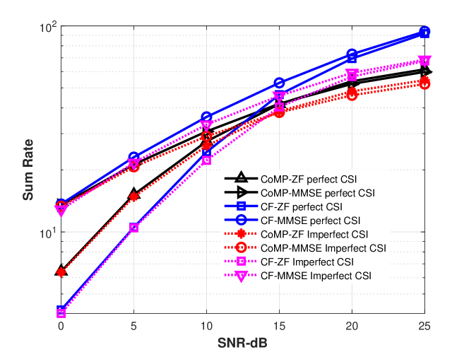
Figure 1: Performance comparison of cell-free and multicell networks considering all users

Figs. 2 and 3 show how different scheduling methods work in cell-free and multicell networks, respectively, when the sum-rate criterion is used. We have compared the performance of the systems implementing an exhaustive search, the proposed enhanced greedy and ZFS user scheduling algorithms to schedule half of the users when ZF and MMSE precoders are used. According to these figures, the proposed enhanced greedy method achieves an impressive improvement compared with ZFS and its performance is very close to the optimal exhaustive search method in cell-free networks. For multicell networks we also have a significant improvement. The performance of cell-free and multicell networks using the proposed enhanced greedy algorithm is also shown in Fig. 4, where the cell-free system has outperformed the multicell system, as expected.

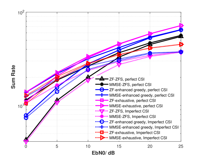
Figure 2: Performance of cell-free network with different scheduling methods

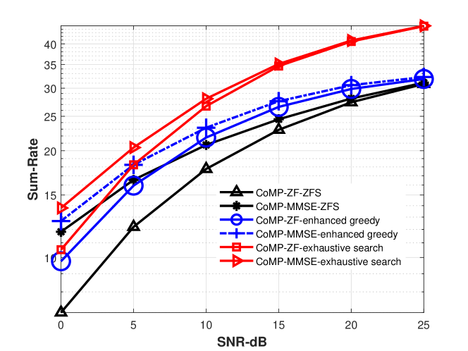
Figure 3: Performance of multicell network with different scheduling methods

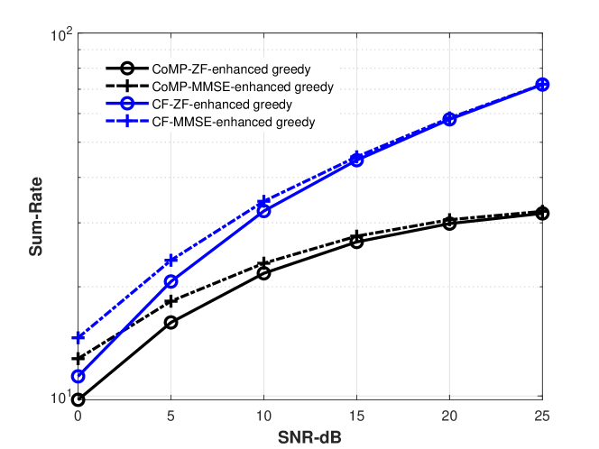
Figure 4: Performance comparison of cell-free and multicell networks using the proposed enhanced greedy method

In Fig. 5, the performance of the enhanced greedy algorithm in a cell-free network is shown when the sum-rate and channel-correlation criteria are used. We can see that using the sum-rate criterion provide an improvement in system performance while the results for the channel-correlation criterion are slighltly worse. The choice of the sum-rate and the channel-correlation criteria depends on the available computational power and application.

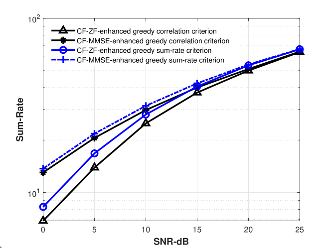
Figure 5: Performance of the enhanced greedy algorithm in a cell-free network for sum-rate and channel-correlation criteria

In Table II, the computational complexity of the ZFS and the proposed enhanced greedy methods for the sum-rate and channel-correlation criteria are shown in cellular and cell-free networks with network-centring clustering. The results show that the improvement in the method using the sum-rate criterion comes at the cost of more required flops.

TABLE II: Computational Complexity

	Multicell flops	Cell-free flops
ZFS	3580	3580
Enhanced greedy (channel-correlation)	9484	9484
Enhanced greedy (sum capacity)	12148	12148

V Conclusion

We have proposed an enhanced greedy algorithm that extends the search procedure to find the user set with the best performance in cell-free and multicell MIMO systems. Numerical results show that there is a significant performance improvement in both cell-free and multicell systems using the proposed algorithm while linear MMSE and ZF precoders were used. The sum-rate criterion in the proposed enhanced greedy algorithm has outperformed the channel-correlation criterion at the cost of a slight increase in computational complexity.

References

- [1] W. Chen, P. Hsieh, and B. Chen, “Multi-objective power minimization design for energy efficiency in multicell multiuser mimo beamforming system,” IEEE Transactions on Green Communications and Networkings, vol. 4, no. 1, pp. 31–45, 2020.
- [2] X. Nguyen and H. H. Kha, “Energy efficient full-duplex multicell multi-user mimo networks,” International Conference on Advanced Technologies for Communications (ATC), pp. 163–167, 2018.
- [3] K. K. Wong, G. Liu, W. Cun, W. Zhang, M Zhao, and Z. Zheng, “Truly distributed multicell multi-band multiuser mimo by synergizing game theory and deep learning,” IEEE Access, vol. 9, pp. 30347–30358, 2021.
- [4] Rodrigo C. de Lamare, “Massive mimo systems: Signal processing challenges and future trends,” URSI Radio Science Bulletin, vol. 2013, no. 347, pp. 8–20, 2013.
- [5] Wence Zhang, Hong Ren, Cunhua Pan, Ming Chen, Rodrigo C. de Lamare, Bo Du, and Jianxin Dai, “Large-scale antenna systems with ul/dl hardware mismatch: Achievable rates analysis and calibration,” IEEE Transactions on Communications, vol. 63, no. 4, pp. 1216–1229, 2015.
- [6] Yunlong Cai, Rodrigo C. de Lamare, Lie-Liang Yang, and Minjian Zhao, “Robust mmse precoding based on switched relaying and side information for multiuser mimo relay systems,” IEEE Transactions on Vehicular Technology, vol. 64, no. 12, pp. 5677–5687, 2015.
- [7] Xiaotao Lu and Rodrigo C. de Lamare, “Opportunistic relaying and jamming based on secrecy-rate maximization for multiuser buffer-aided relay systems,” IEEE Transactions on Vehicular Technology, vol. 69, no. 12, pp. 15269–15283, 2020.
- [8] Keke Zu, Rodrigo C. de Lamare, and Martin Haardt, “Generalized design of low-complexity block diagonalization type precoding algorithms for multiuser mimo systems,” IEEE Transactions on Communications, vol. 61, no. 10, pp. 4232–4242, 2013.
- [9] Wence Zhang, Rodrigo C. de Lamare, Cunhua Pan, Ming Chen, Jianxin Dai, Bingyang Wu, and Xu Bao, “Widely linear precoding for large-scale mimo with iqi: Algorithms and performance analysis,” IEEE Transactions on Wireless Communications, vol. 16, no. 5, pp. 3298–3312, 2017.
- [10] Patrick Clarke and Rodrigo C. de Lamare, “Transmit diversity and relay selection algorithms for multirelay cooperative mimo systems,” IEEE Transactions on Vehicular Technology, vol. 61, no. 3, pp. 1084–1098, 2012.
- [11] Rodrigo C. De Lamare and Raimundo Sampaio-Neto, “Minimum mean-squared error iterative successive parallel arbitrated decision feedback detectors for ds-cdma systems,” IEEE Transactions on Communications, vol. 56, no. 5, pp. 778–789, 2008.
- [12] Lukas T. N. Landau and Rodrigo C. de Lamare, “Branch-and-bound precoding for multiuser mimo systems with 1-bit quantization,” IEEE Wireless Communications Letters, vol. 6, no. 6, pp. 770–773, 2017.
- [13] Yunlong Cai, Rodrigo C. de Lamare, and Rui Fa, “Switched interleaving techniques with limited feedback for interference mitigation in ds-cdma systems,” IEEE Transactions on Communications, vol. 59, no. 7, pp. 1946–1956, 2011.
- [14] Cornelius T. Healy and Rodrigo C. de Lamare, “Design of ldpc codes based on multipath emd strategies for progressive edge growth,” IEEE Transactions on Communications, vol. 64, no. 8, pp. 3208–3219, 2016.
- [15] Andre G. D. Uchoa, Cornelius Healy, Rodrigo C. de Lamare, and Richard D. Souza, “Design of ldpc codes based on progressive edge growth techniques for block fading channels,” IEEE Communications Letters, vol. 15, no. 11, pp. 1221–1223, 2011.
- [16] Jiaqi Gu, Rodrigo C. de Lamare, and Mario Huemer, “Buffer-aided physical-layer network coding with optimal linear code designs for cooperative networks,” IEEE Transactions on Communications, vol. 66, no. 6, pp. 2560–2575, 2018.
- [17] Keke Zu, Rodrigo C. de Lamare, and Martin Haardt, “Multi-branch tomlinson-harashima precoding design for mu-mimo systems: Theory and algorithms,” IEEE Transactions on Communications, vol. 62, no. 3, pp. 939–951, 2014.
- [18] Lei Zhang, Yunlong Cai, Rodrigo C. de Lamare, and Minjian Zhao, “Robust multibranch tomlinson–harashima precoding design in amplify-and-forward mimo relay systems,” IEEE Transactions on Communications, vol. 62, no. 10, pp. 3476–3490, 2014.
- [19] Andre R. Flores, Rodrigo C. de Lamare, and Bruno Clerckx, “Linear precoding and stream combining for rate splitting in multiuser mimo systems,” IEEE Communications Letters, vol. 24, no. 4, pp. 890–894, 2020.
- [20] Andre R. Flores, Rodrigo C. De Lamare, and Bruno Clerckx, “Tomlinson-harashima precoded rate-splitting with stream combiners for mu-mimo systems,” IEEE Transactions on Communications, vol. 69, no. 6, pp. 3833–3845, 2021.
- [21] Hang Ruan and Rodrigo C. de Lamare, “Distributed robust beamforming based on low-rank and cross-correlation techniques: Design and analysis,” IEEE Transactions on Signal Processing, vol. 67, no. 24, pp. 6411–6423, 2019.
- [22] Victoria M. T. Palhares, Andre R. Flores, and Rodrigo C. de Lamare, “Robust mmse precoding and power allocation for cell-free massive mimo systems,” IEEE Transactions on Vehicular Technology, vol. 70, no. 5, pp. 5115–5120, 2021.
- [23] Diana M. V. Melo, Lukas T. N. Landau, Rodrigo C. De Lamare, Peter F. Neuhaus, and Gerhard P. Fettweis, “Zero-crossing precoding techniques for channels with 1-bit temporal oversampling adcs,” IEEE Transactions on Wireless Communications, pp. 1–1, 2023.
- [24] W. Wang, A. Harada, and H. Kayama, “Enhanced limited feedback schemes for dl mu-mimo zf precoding,” IEEE Transactions on Wireless Communications, vol. 12, no. 4, pp. 1554–1561, 2013.
- [25] C. Chen, H. Tsao, and P. Tsai, “Equal-rate qr decomposition based on mmse technique for multi-user mimo precoding,” IEEE 24th Annual International Symposium on Personal, Indoor, and Mobile Radio Communications (PIMRC), pp. 435–440, 2013.
- [26] D. H. Nguyen, L. B. Le, T. Le-Ngoc, and R. W. Heath, “Hybrid mmse precoding and combining designs for mmwave multiuser systems,” IEEE Access, vol. 5, pp. 19167–19181, 2017.
- [27] M. Wang and L. M. Davis, “Distributed user selection in multi-cell massive mimo systems with pilot contamination,” IEEE 82nd Vehicular Technology Conference (VTC2015-Fall), pp. 1–5, 2015.
- [28] S. E. Hajri, M. Assaad, and G. Caire, “Scheduling in massive mimo: User clustering and pilot assignment,” 2016 54th Annual Allerton Conference on Communication, Control, and Computing (Allerton), pp. 107–114, 2016.
- [29] T. L. Marzetta, “Noncooperative cellular wireless with unlimited numbers of base station antennas,” IEEE Transactions on Wireless Communications, vol. 9, no. 11, pp. 590–3600, 2010.
- [30] M. Wang and L. M. Davis, “On downlink beamforming with greedy user selection: performance analysis and a simple new algorithm,” IEEE Transactions on Signal Processing, vol. 53, no. 10, pp. 3857–3868, 2005.
- [31] M. Wang, T. Samarasinghe, and J. S. Evans, “Optimizing user selection schemes in vector broadcast channels,” IEEE Transactions on Communications, vol. 63, no. 2, pp. 565–577, 2015.
- [32] Z. Huo, N. Ma, and B. Liu, “Joint user scheduling and transceiver design for cross-link interference suppression in mu-mimo dynamic tdd systems,” 3rd IEEE International Conference on Computer and Communications (ICCC), pp. 962–967, 2017.
- [33] H. Q. Ngo, A. Ashikhmin, H. Yang, E. G. Larsson, and T. L. Marzetta, “Cell-free massive mimo: Uniformly great service for everyone,” 2015 IEEE 16th International Workshop on Signal Processing Advances in Wireless Communications (SPAWC), pp. 201–205, 2015.
- [34] H. Q. Ngo, A. Ashikhmin, H. Yang, E. G. Larsson, and T. L. Marzetta, “Cell-free massive mimo versus small cells,” IEEE Transactions on Wireless Communications, vol. 16, no. 3, pp. 1834–1850, 2017.
- [35] E. Nayebi, A. Ashikhmin, T. L. Marzetta, H. Yang, and B. D. Rao, “Precoding and power optimization in cell-free massive mimo systems,” IEEE Transactions on Wireless Communications, vol. 16, no. 7, pp. 4445–4459, 2017.
- [36] E. Björnson and L. Sanguinetti, “Cell-free versus cellular massive mimo: What processing is needed for cell-free to win?,” IEEE 20th International Workshop on Signal Processing Advances in Wireless Communications (SPAWC), pp. 1–5, 2019.
- [37] E. Björnson and L. Sanguinetti, “Scalable cell-free massive mimo systems,” IEEE Transactions on Communications, vol. 68, no. 7, pp. 4247–4261, 2020.
- [38] Saeed Mashdour, Rodrigo C. de Lamare, and João P. S. H. Lima, “Enhanced subset greedy multiuser scheduling in clustered cell-free massive mimo systems,” IEEE Communications Letters, vol. 27, no. 2, pp. 610–614, 2023.
- [39] P. Li and R. C. de Lamare, “Distributed iterative detection with reduced message passing for networked mimo cellular systems,” IEEE Transactions on Vehicular Technology, vol. 63, no. 6, pp. 2947–2954, 2014.
- [40] A. Tang, J. Sun, and K. Gong, “Mobile propagation loss with a low base station antenna for nlos street microcells in urban area,” IEEE VTS 53rd Vehicular Technology Conference, Spring 2001. Proceedings (Cat. No.01CH37202), vol. 1, pp. 333–336, 2001.
- [41] Z. Shen, R. Chen, J. G. Andrews, R. W. Heath, and B. L. Evans, “Low complexity user selection algorithms for multiuser mimo systems with block diagonalization,” IEEE Transactions on Signal Processing, vol. 54, no. 9, pp. 3658–3663, 2006.
- [42] X. Zhang and J. Lee, “Low complexity mimo scheduling with channel decomposition using capacity upperbound,” IEEE Transactions on Communications, vol. 56, no. 6, pp. 871–876, 2008.
- [43] S. Sigdel and W. A. Krzymien, “Simplified fair scheduling and antenna selection algorithms for multiuser mimo orthogonal space-division multiplexing downlink,” IEEE Transactions on Vehicular Technology, vol. 58, no. 3, pp. 1329–1344, 2009.