Modular Quantization-Aware Training:
Increasing Accuracy by Decreasing Precision in 6D Object Pose Estimation

Abstract

Edge applications, such as collaborative robotics and spacecraft rendezvous, demand efficient 6D object pose estimation on resource-constrained embedded platforms. Existing 6D pose estimation networks are often too large for such deployments, necessitating compression while maintaining reliable performance. To address this challenge, we introduce Modular Quantization-Aware Training (MQAT) ,an adaptive and mixed-precision quantization-aware training strategy that exploits the modular structure of modern 6D pose estimation architectures. MQAT guides a systematic gradated modular quantization sequence and determines module-specific bit precisions, leading to quantized models that outperform those produced by state-of-the-art uniform and mixed-precision quantization techniques. Our experiments showcase the generality of MQAT across datasets, architectures, and quantization algorithms. Remarkably, MQAT-trained quantized models achieve a significant accuracy boost ($>7\%$) over the baseline full-precision network while reducing model size by a factor of $4\times$ or more.

1 Introduction

Efficient and reliable 6D pose estimation has emerged as a crucial component in numerous situations, particularly in robotics applications such as automated manufacturing [35], vision-based control [43], collaborative robotics [50] and spacecraft rendezvous [45]. However, such applications typically must run on embedded platforms with limited hardware resources.

These resource constraints largely disqualify the recent state-of-the-art methods, such as ZebraPose [46], SO-Pose [11], and GDRNet [51], which employ a two stage approach (detection followed by pose estimation) and thus entail a large memory footprint. By contrast, single-stage methods [49, 34, 44, 21, 52, 7, 41, 17] offer a more pragmatic alternative, yielding models with a good accuracy-footprint tradeoff. Nevertheless, these models remain too large for deployment on edge devices.

To address this challenge, CA-SpaceNet [52] applies a uniform quantization approach to reduce the network memory footprint at the expense of a large accuracy loss; all network layers are quantized to the same bit width, except for the first and last layer. In principle, mixed-precision quantization methods [6, 13, 47] could demonstrate similar compression with better performance, but they tend to require significant effort and GPU hours to determine the optimal bit precision for each layer. Furthermore, neither mixed-precision nor uniform quantization methods consider the importance of the order in which the network weights or layers are quantized, as searching for the optimal order is combinatorial in the number of, e.g., network layers.

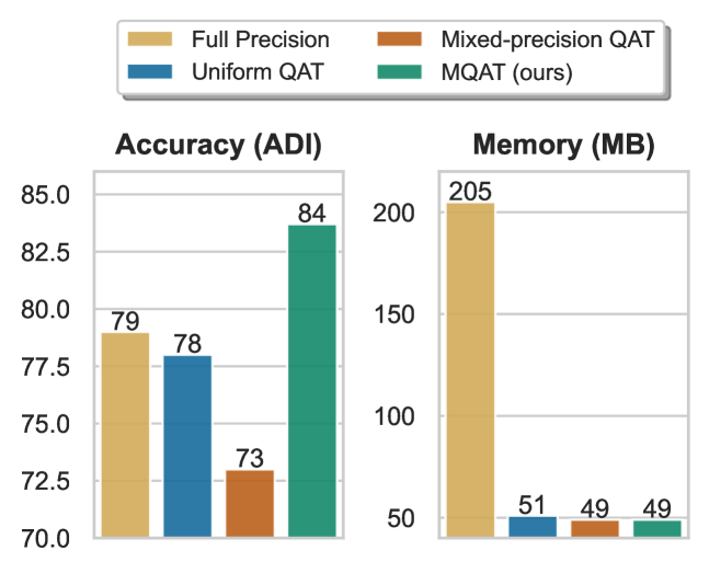
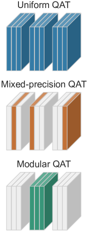
Figure 1: Summary of this Work. In contrast to uniform and mixed-precision quantization, MQAT accounts for the modularity of typical 6D pose estimation frameworks. MQAT not only reduces the memory footprint of the network but can result in an accuracy boost that neither uniform nor mixed-precision quantization have demonstrated.

In this work, we depart from such conventional Quantization-Aware Training (QAT) approaches and leverage the inherent modular structure of modern 6D object pose estimation architectures, which typically encompass components such as a backbone, a feature aggregation module, and prediction heads. Specifically, we introduce a Modular Quantization-Aware Training (MQAT) paradigm that relies on a gradated quantization strategy, where the modules are quantized and fine-tuned in a mixed-precision way, following a sequential order based on their sensitivity to quantization. As the number of modules in an architecture is much lower than that of layers, our approach allows us to search for the optimal quantization order.

Our experiments evidence that MQAT is particularly well-suited to 6D pose estimation, consistently outperforming the state-of-the-art quantization techniques in terms of accuracy for a given memory consumption budget, as shown in Figure 1. Furthermore, we show that MQAT can even yield an accuracy boost over the original full-precision network, which none of the existing quantization methods can achieve.

We also demonstrate the generality of our approach by applying it to different single-stage architectures, WDR [21], CA-SpaceNet [52]; different datasets, SwissCube [21], Linemod [16], and Occlusion Linemod [4]; and using different quantization strategies, INQ [59] and LSQ [14], within our modular strategy. We further show that our method also applies to two-stage networks, such as ZebraPose [46], on which it outperforms both uniform and mixed-precision quantization.

To summarize, our main contributions are as follows:

• We develop a Modular Quantization-Aware Training (MQAT) paradigm, a novel method that enhances 6D object pose estimation accuracy through adaptive, mixed-precision quantization tailored for modular neural network architectures.

• We demonstrate substantial accuracy gains over other Quantization-Aware Training methods and even surpass full-precision counterparts in case of single-stage networks [21, 52], while significantly reducing the computational cost and model size, showcasing the effectiveness of MQAT in balancing precision and performance.

• We validate the MQAT method across multiple datasets and neural network architectures, proving its adaptability and effectiveness in different settings and its potential for broad application in the field of pose estimation.

• We provide comprehensive studies offering insights into the impact of module-specific order and bit precision on network performance. This includes detailed ablation studies that establish the superiority of MQAT over existing quantization methods.

2 Related Work

In this section, we survey the recent advances in RGB-based 6D pose estimation, outlining key architectures and their contributions to the field. We then explore the developments in quantization-aware training (QAT), particularly in relation to modular neural network designs. This review sets the groundwork for our proposed Modular Quantization-Aware Training framework, which is inspired by these advances and addresses their limitations.

2.1 6D Pose Estimation

Single-Stage Direct Estimation. PoseCNN [53] was one of the first methods to estimate 6D object pose using a deep neural network. The network comprised a backbone feature extractor which fed into three heads: a labeller, a segmenter and a fully-connected head to regress the pose directly. Unfortunately, representing the $SO(3)$ group rotations in a manner suitable for direct regression proved to be challenging. SSD6D [30, 25] instead proposed a discretization of the rotation space to form a classification problem instead of a regression one. URSONet [40], and more recently Mobile-URSONet [39], demonstrated competitive results via a backbone–bottleneck–head structure to estimate the weights of a set of classification quaternions corresponding to Euler angle rotations.

Single-Stage with PnP. In general, a better performing strategy consists of training a network to predict 2D-to-3D correspondences instead of the pose. The pose is then obtained via a RANdom SAmple Consensus (RANSAC) / Perspective-n-Point (PnP) 2D–to–3D correspondence fitting process. These methods typically employ a backbone, a feature aggregation module, and one or multiple heads [21, 7, 41, 52, 34, 48, 49, 22, 56, 33, 24, 20]. [41, 48] estimate these correspondences in a single global fashion, whereas [34, 24, 20, 56, 33] aggregate multiple local predictions to improve robustness. To improve performance in the presence of large depth variations, a number of works [49, 21, 52] use an FPN [29] to exploit features at different scales.

Multi-Stage with PnP. The current state-of-the-art pose estimation frameworks incorporate a pipeline of networks that perform different tasks [46, 11, 51, 28, 26]. In the first stage network, the target is localized and a Region of Interest (RoI) is cropped and forwarded to the second stage network. This isolates the position estimation task from the orientation estimation one and further provides the orientation estimation network with an RoI containing only object features. The second stage orientation estimation network can then more easily fit to the target object. Therefore, these multi-stage frameworks tend to yield more accurate results. However, they also have much larger memory footprints as they may include one object classifier network; one object position/RoI network; and $N$ object pose networks. For hardware-restricted scenarios, a multi-stage framework may thus not be practical. Even for single-stage networks, additional compression is required [3].

2.2 Quantization-Aware Training

Neural network quantization reduces the precision of parameters such as weights and activations. Existing techniques fall into two broad categories: Post-training quantization (PTQ) [32, 27, 15, 58, 5, 31] and quantization-aware training (QAT). The latter further divides into uniform QAT [14, 59, 2, 54] and mixed-precision QAT [6, 13, 47, 12, 8, 55]. While PTQ avoids the laborious training step, QAT exploits the training and thus better preserves the model’s full-precision accuracy. As accuracy can be critical in robotics applications relying on 6D object pose estimation, we focus on QAT.

Uniform QAT methods quantize every layer of the network to the same precision. In Incremental Network Quantization (INQ) [59], this is achieved by quantizing a uniform fraction of each layers’ weights at a time and continuing training until the next quantization step. Quantization can be achieved in a structured manner, where entire kernels are quantized at once, or in an unstructured manner. In contrast to INQ, Learned Step-size Quantization (LSQ) [14] quantizes the entire network in a single action. To this end, LSQ treats the quantization step-size as a learnable parameter. The method then alternates between updating the weights and the step-size parameter.

Mixed-precision QAT methods, conversely, treat each network layer uniquely, aiming to determine the appropriate bit precision for each one. In HAWQ [12, 13, 55], the network weights’ Hessian is leveraged to assign bit precisions proportional to the gradients. In [6], the mixed precision is taken even further by applying a different precision to different kernels within a single channel. Mixed-precision QAT is a challenging task; existing methods remain computationally expensive for modern deep network architectures.

2.3 Quantization and Modular Deep Learning

In recent years, deep network architectures have increasingly followed a modular paradigm, owing to its advantages in model design and training efficiency [23, 38, 1, 19, 37]. This approach leverages reusable modules, amplifying the flexibility and adaptability of neural networks and fostering parameter-efficient fine-tuning.

In the quantization domain, several studies have underscored the importance of selecting the appropriate granularity to bolster model generalization [27] and enhance training stability [57]. To our knowledge, no existing research has advocated a systematic methodology for executing modular quantization-aware training, let alone studied the impact of quantization order on modular architectures. Furthermore, in the 6D pose estimation domain, the application of quantization remains limited [52], with none of the aforementioned quantization techniques addressing the specific task or underlying network architecture. Thus, in this work, we aim to bridge this gap by introducing a comprehensive methodology for modular quantization-aware training, tailored but not limited to 6D pose estimation.

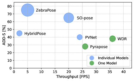
Figure 2: Performance Comparison on O-LINEMOD. The marker size is proportional to the memory footprint. Individual Models refers to methods training individual models for each object. One Model refers to methods training a single model for all objects.

3 Method

In this section, we first describe the general type of network architecture we consider for compact 6D pose estimation and then introduce our Modular Quantization-Aware Training (MQAT) method.

3.1 Network Architecture

As discussed in Section 2, multi-stage networks [46, 11, 51, 26, 28] tend to induce large memory footprints and large latencies, thus making poor candidates for hardware-restricted applications. This is further evidenced in Figure 2, where we compare a number of 6D pose estimation architectures’ memory footprint, throughput and accuracy on the O-LINEMOD dataset. While demonstrating admirable accuracy, the size and latency of ZebraPose [46] and SO-pose [11] preclude their inclusion in hardware-restricted platforms.

On this basis, we therefore focus on single-stage 6D pose estimation networks [49, 52, 48, 34, 21]. In general, such networks consist of multiple modules, exhibiting an encoder-decoder structure followed by prediction heads. Examples include PyraPose [49], WDR[21], and CA-SpaceNet [52]; a representative generic architecture is illustrated in Figure 3.

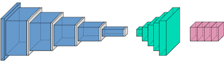
Figure 3: Representative 6D Pose Estimation Network with $K=3$ modules. From left to right, we denote them as backbone, feature aggregation, and heads.

3.2 MQAT Overview

Coventional Quantization Aware Training (QAT) methods [14, 59, 2, 54] treat each layer of the network uniformly during quantization. While this effectively reduces the network’s memory footprint, it tends to degrade its performance as quantization becomes increasingly aggressive, such as with ternary weights {-1,0,1}. Here, we propose to exploit the modular structure of 6D pose estimation networks to quantize each module differently, resulting in a non-uniform quantization strategy. As shown below, MQAT requires minimal effort to implement compared to a mixed-precision quantization method [6, 47, 9, 55].

Specifically, MQAT begins by performing aggressive quantization (i.e., ternary weights) with a modified uniform QAT method (e.g., INQ [59], LSQ [14]) on a single module of the network. This process is repeated for all $K$ modules, where only the $k^{\rm th}$ module is quantized while the remaining $K-1$ modules retain full precision. The quantization of only a selected module $B_{k}$ provides flexibility for the other $K-1$ full precision modules to compensate for any accuracy loss; in some cases accuracy even improves as will be shown in Section 4.

Given the aggressive quantization sensitivity results for each individual module, $B_{k}$, we define an optimal quantization order, which we thereafter refer to as the quantization flow. We then sequentially quantize the modules in the optimal order, with the optimal bit precision, determined using constrained optimization. The resulting MQAT strategy is provided in Algorithm 1 and described in more detail below. The results of MQAT in conjunction with LSQ and INQ will be demonstrated in Section 4. Note that any traditional QAT algorithm can be applied as the quantization method $Q$, in lieu of INQ or LSQ.

3.3 Algorithmic Details

Let us now introduce our MQAT algorithm, as depicted in Algorithm 1 (where we also defined the notations). We begin by introducing the critical components for our approach.

Algorithm 1 MQAT Algorithm

Input: Training data
Input: Quantization $Q$
Input: Model $M$, with modules $\textbf{B}=[B_{1},B_{2},...,B_{K}]$
Input: Bit-width search $q=[2,4,8...]$
Input: Model accuracy metric $ac(M)$

1:for $k=1,2,..K$ do

2:     $M_{k}^{2}\leftarrow Q_{k}^{2}(M)$

3:     if $ac(M_{k}^{2})>ac(M)\land ac(M_{k}^{2})>ac(M_{best})$ then

4:         $M_{best}\leftarrow M_{k}^{2}$

5:         $k_{best}\leftarrow k$

6:     end if

7:end for

8:$flow=[\hskip 2.0pt]$

9:if $M_{best}$ then

10:     $M\leftarrow M_{best}$

11:     $flow\leftarrow index(SORT\_SIZE(\textbf{B}))$

12:     $flow.pop(k_{best})$

13:else

14:     $flow\leftarrow index(SORT\_SIZE(\textbf{B}))$

15:end if

16:$\rho\leftarrow ILP(M,q)$

17:$i\leftarrow 0$

18:while $i<=len(flow)$ do

19:     $M^{Q}\leftarrow Q_{flow(i)}^{\rho(i)}(M)$

20:     retrain($M^{Q}$)

21:end while

Output: Modular quantized model ($M^{Q}$).

$flow$

Sequence of quantization order of modules.

$k_{best}$

Index of the quantized module which increased performance.

$K$

Number of modules

$M_{best}$

Highest accuracy model containing a quantized module.

$M_{k}^{q}$

Model with only module $k$ quantized to $q$ bits.

$M^{Q}$

Model with modules quantized to differet bit precisions.

$\rho$

List of bit precisions for each module.

$Q_{c}^{j}$

Quantization applied to module $B_{c}$ with $j$-bits.

Quantization Flow (Lines 1:15). For a modular network with $K$ modules, we conduct $K$ independent 2 bit quantizations for each module. A module $B_{k}^{q}$ ($B_{k}$ quantized to bit-precision $q$) is retained if it results in an improved accuracy for $M_{k}^{q}$ (Model with only $B_{k}$ quantized to bit-precision $q$), providing a baseline for the appropriate bit precision optimization. The sequence of module quantization is critical since quantizing the modules of a network is not commutative; we prioritize starting with modules that do not compromise accuracy, as errors introduced early on are typically not mitigated by later steps. Moreover, we also observe that quantization-related noise can lead to weight instability [10, 42, 36], hindering the performance of the quantized network.

If no quantized module yields an improved accuracy, we proceed with quantizing the module with the lowest number of parameters first; the modules with higher parameter numbers will have more flexibility to adapt to aggressive quantization. The resulting optimal quantization flow is then passed to the next algorithmic step.

Optimal Bit Precision (Lines 16:21). In MQAT, the optimal bit precision for each module is ascertained through a process of constrained optimization, Integer Linear Programming (ILP), drawing inspiration from [55]. However, our methodology distinguishes itself by offering a lower degree of granularity. Central to our strategy is the uniform quantization of all layers within a given module to an identical bit-width. This design choice not only simplifies the computational complexity but also significantly enhances the hardware compatibility of the system, an essential consideration for efficient real-world deployment.

To achieve this, we introduce the importance metric for modular quantization. This metric is conceptualized as the product of two factors: the sensitivity metric, $\lambda$, for each layer in a module which is computed by a similar approach to that in [13], and the quantization weight error. The latter is calculated as the squared 2-norm difference between the quantized and full precision weights. Therefore, the importance metric is given by

$$\Omega_{k}=\frac{1}{L_{k}}\sum_{i=1}^{L_{k}}\frac{\lambda_{i}}{N_{i}}\left|Q\left(W_{i}\right)-W_{i}\right|_{2}^{2},$$ (1)

with

   $k$

the $k$-th module in the modular network;

   $i$

the $i$-th layer within module $k$;

   $L_{k}$

the total number of layers in module $k$;

   $N_{i}$

the number of parameters in the $i$-th layer of module $k$;

   $\lambda_{i}$

the sensitivity of the $i$-th layer in module $k$;

   $Q$

the quantization operation;

   $W_{i}$

the weights of the $i$-th layer in module $k$.

Finding optimal bit precisions using ILP is formulated as

$$\begin{split}&\min_{\left\{\rho_{k}\right\}_{k=1}^{K}}\sum_{k=1}^{K}\Omega_{k}^{\left(\rho_{k}\right)},\\ \text{subject to}&~{}~{}\sum_{k=1}^{K}S_{k}^{\left(\rho_{k}\right)}\leq\frac{\text{Full Precision Model Size}}{\text{Compression factor}}\;.\end{split}$$ (2)

In this formulation, $\rho_{k}$ denotes the bit-width for the $k^{th}$ module; $S_{k}$ denotes the model size of module $k$; and $K$ represents the total number of layers.

4 Experiments

Historically, quantization and other compression methods have been used to exercise a trade-off between inference accuracy and deployment feasibility, particularly in resource-constrained circumstances. In the following sections, we will show that our approach may yield a significant inference accuracy improvement during compression. To the best of our knowledge, this is the first time quantization has demonstrated such a consistent enhancement.

We first introduce the datasets and metrics used for evaluation. Then, we present ablation studies to explore the nature of MQAT enhancing network accuracy; this result is directly compared to uniform and mixed QAT methods. Finally, we demonstrate the generality of our method applied to different datasets, architectures, and QAT methods.

4.1 Datasets and Metrics

The LINEMOD and O-LINEMOD datasets are standard benchmarks for evaluating 6D pose estimation methods, where the LINEMOD dataset contains 13 different sequences consisting of ground-truth poses for a single object. Similar to GDRNet [51], we utilize 15% of the images for training. O-LINEMOD extends LINEMOD by including occlusions. For both datasets, additional rendered images are used during training [51, 34]. Similarly to previous works, we use the ADD and ADI error metrics [18] expressed as

$$e_{ADD}(P^{est},P^{gt})=\frac{1}{V}\sum_{i=1}^{V}\lVert P^{est}_{i}-P^{gt}_{i}\rVert_{2}\;,$$ (3)

$$e_{ADI}(P^{est},P^{gt})=\frac{1}{V}\sum_{i=1}^{V}\;\;\underset{j\in[1,V]}{\rm min}\lVert P^{est}_{i}-P^{gt}_{j}\rVert_{2}\;,$$ (4)

where $P^{est}_{i}$ and $P^{gt}_{i}$ denote the $i^{th}$ vertex of the 3D mesh model after transformation with the predicted and ground-truth pose, respectively. We then report the accuracy using the ADD-0.1d and ADD-0.5d metrics, which encode the proportion of samples for which $e_{ADD}$ is less than 10% and 50% of the object diameter, respectively.

While LINEMOD and O-LINEMOD present their own set of challenges, their scope is restricted to household objects, consistently illuminated without significant depth variations. Conversely, the SwissCube dataset [21] embodies a challenging scenario for 6D pose estimation in space, incorporating large scale variations, diverse lighting conditions, and variable backgrounds. To remain consistent with previous works, we use the same training setup and metric as [52]. The robustness of MQAT for 6D pose estimation is thus demonstrated on diverse datasets.

4.2 Implementation Details

We use PyTorch to implement our method. For the retraining of our partially quantized pretrained network, we employ an SGD optimizer with a base learning rate of 1e-2. For all experiments, we use a batch size of 8, train for 30 epochs, and employ a hand-crafted learning scheduler which decreases the learning rate at regular intervals by a factor of 10 and increases it again when we quantize a module with INQ. However, when we quantize our modules using LSQ, the learning rate factor is not increased, only decreased by factors of 10. We use a $512\times 512$ resolution input for the SwissCube dataset and $640\times 480$ for LINEMOD and O-LINEMOD as in [34].

Figure 4: Aggressive Quantization for Order Optimality.

4.3 MQAT Paradigm Studies

In this section, we conduct comprehensive studies using the SwissCube dataset and demonstrate the superior performance of our paradigm over conventional QAT approaches.

4.3.1 MQAT Order

We first perform an ablation study to validate the optimal order for quantizing the network modules. As discussed in Section 3.3, the module quantization order is not commutative. Using WDR, we perform aggressive quantization to every combination of modules in the network. This is an $O(2^{K})$ search; this results in eight module quantization combinations for a network with $K=3$ modules. The results are visualized in Figure 4. The backbone and head modules exhibit greater sensitivity to aggressive quantization. Conversely, the accuracy of the network is enhanced when using 2 bit quantization on the Feature Pyramid Network (FPN) module only. No other combination of module quantizations yields an accuracy increase. This further emphasizes the importance of carefully selecting a module quantization flow. Note that extending this study by quantizing more modules simultaneously simply converges to a uniform QAT method.

MQAT	ADI
First Quantized Module	0.1d	0.5d
Full Precision	78.79	98.98
Backbone	69.08	96.79
Head	67.84	98.12
Feature Pyramid Network (FPN)	83.8	99.4

Table 1: Effect of Starting MQAT with Different Modules.

We additionally perform ablation studies on the optimal order (i.e., flow) of module quantization. We begin by quantizing different modules first, instead of the FPN. Table 1 shows the results of both the head and backbone modules when they are the first module quantized. We observe that the inference accuracy decreases dramatically for both cases. No combination of module flow or bit precision schedule is able to recover the inference accuracy after it was lost. The 2 bit aggressive FPN quantization yields improved accuracy only when the FPN is quantized first.

4.3.2 Quantized FPN Sensitivity Study

To expand upon the 2 bit FPN accuracy enhancement, we perform a higher granularity bit-precision search on the FPN module. Again, the FPN module was quantized, but to five different bit-widths for comparison; the results are presented in Figure 5. The accuracy of two full-precision networks, WDR [21] and CA-SpaceNet [52], are shown with dashed lines. The highest accuracy is achieved with a 2 bit or ternary $\{-1,0,1\}$ FPN. Further pushing the FPN to binary weights $\{-1,1\}$ slightly reduces the accuracy, but maintains a significant improvement over both baselines.

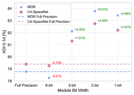
Figure 5: Ablation study on the FPN bit-width. We compare the performance by varying the bit-width of the feature aggregation module in each model.

As shown in Figure 5, our findings reinforce the notion that the integration of low bit-precision quantization within the FPN acts as an effective regularizer. The improvements in performance also underscore the effectiveness of MQAT in enhancing model generalizability.

4.3.3 MQAT Compared to Uniform and Mixed QAT

Historically, QAT methods do not significantly enhance network inference accuracy, and we demonstrate this again here. In a typical hardware-limited application, a suitable network is selected and then compressed to meet the hardware constraints. For direct comparison, we apply three different quantization paradigms. Starting from a full precision WDR network, we apply a uniform QAT method, LSQ [14], a mixed-precision QAT method, HAWQ-V3 [55], and finally our proposed MQAT method with increasing compression factors. The results are provided in Figure 7. Again, MQAT demonstrates a significant accuracy improvement while sustaining the requested compression factor; it is the only quantization approach to show an increase in inference accuracy during compression.

Figure 6: Comparison between our proposed paradigm MQAT, uniform QAT (LSQ), and layer-wise mixed-precision QAT (HAWQ-V3).

4.4 MQAT Generality

Finally, we demonstrate the generality of MQAT to different datasets, QAT methods, and network architectures.

MQAT Mode	Bit-Precisions	SwissCube		LINEMOD		O-LINEMOD
		0.1d	0.5d	0.1d	0.5d	0.1d	0.5d
Full precision	Full precision	78.8	98.9	56.1	99.1	37.8	85.2
MQATLSQ	8-2-8	83.4	99.3	63.5	99.2	39.8	86.4
MQATINQ	8-2-8	83.7	99.4	63.9	99.5	40.2	86.7

Table 2: Quantized FPN in WDR network on different datasets. Following common practice, we report ADI for Swisscube and ADD for LINEMOD / O-LINEMOD.

4.4.1 Dataset and QAT Generality

As discussed in Section 4.1, the image domains of LINEMOD, O-LINEMOD and SwissCube are vastly different. The full precision and MQAT with 2 bit-precision FPN results for all three datasets are shown in Table 2. MQAT demonstrates an accuracy improvement in all datasets. We use the ADI metric for evaluation on the SwissCube dataset as in [21, 52], while we use the ADD metric for LINEMOD and O-LINEMOD as used by [51, 46, 49, 26, 34].

Accuracy improvements of 5.0%, 7.8% and 2.4% are demonstrated on SwissCube, LINEMOD and O-LINEMOD, respectively, when MQAT with INQ is utilized. Replacing INQ with LSQ yields accuracy improvements of 4.6%, 7.5% and 2.0%, respectively. This evidences that the performance enhancement is independent of the dataset domain and the applied QAT method.

As discussed in Section 3.3 and Section 4.3.1, it is difficult to recover accuracy once it is lost during quantization. To this end, since INQ [59] quantizes only a fraction of the network at once, it follows that the remaining unquantized portion of the network is left flexible to adapt to aggressive quantization. Conversely, LSQ [14] quantizes the entire network in a single step; no fraction of the network is left unperturbed. Consequently, INQ demonstrates superior results in Table 2. While any QAT method may be used, we recommend partnering MQAT with INQ for optimal aggressive quantization results.

Network	Near	Medium	Far	All
SegDriven-Z [20]	41.1	22.9	7.1	21.8
DLR [7]	52.6	45.4	29.4	43.2
CA-SpaceNet	91.0	86.3	61.7	79.4
CA-SpaceNet*	95.5	90.7	66.2	82.7
WDR	92.4	84.2	61.3	78.8
WDR*	96.1	91.5	68.2	83.8

Table 3: Comparison with the state-of-the-art on SwissCube. We report ADI-0.1d scores for 3 different depth ranges. A * indicates applying MQAT with 2 bit precision FPN to the model.

4.4.2 Architecture Generality

In Table 3, we compare several single-stage PnP architectures on the SwissCube dataset. To demonstrate the generality of our performance enhancement, we aggressively quantize the FPN of both CA-SpaceNet [52] and WDR [21]. We demonstrate an accuracy improvement of 4.5%, 4.4% and 4.5% for Near, Medium and Far images, respectively, on CA-SpaceNet, resulting in a total testing set accuracy improvement of 3.3%. Recall the already presented total testing set accuracy improvement of 5.0% for WDR. Previously, the full precision CA-SpaceNet had shown a performance improvement over the full precision WDR, but WDR sees greater gains from the application of MQAT.

Figure 7: Visualization of predictions. Comparison between our proposed MQAT paradigm, and full-precision network. The model applying MQAT yields predictions that are on par with, or more concentrated than its full-precision counterpart.

In addition, [52] published accuracy results for a uniform QAT quantized CA-Space network, shared in Table 4. Specifically, CA-SpaceNet explored three quantization modes (B, BF and BFH). These correspond to quantizing the backbone, quantizing the backbone and FPN (paired), and quantizing the whole network (uniformly), respectively. As we demonstrated in Section 4.3.1, quantizing network modules in pairs greatly reduces inference accuracy as the smaller unquantized fraction of the network is not able to adapt to the quantization. Additionally, quantizing from backbone to head does not consider the sensitivity of the network modules to quantization. As a final note, CA-SpaceNet does not quantize the first and last layer in any quantization mode. In contrast, MQAT quantizes the entire network.

Quantization Method	ADI-0.1d	Compression	Bit-Precisions (B-F-H)
LSQ	79.4	$1\times$	32-32-32
LSQ B	76.2	$2.2\times$	8-32-32
LSQ BF	75.0	$3.2\times$	8-8-32
LSQ BFH	74.7	$4.0\times$	8-8-8
MQAT (Ours)	82.7	$4.7\times$	8-2-8
LSQ B	75.1	$2.9\times$	3-32-32
LSQ BF	74.5	$5.9\times$	3-3-32
MQAT (Ours)	80.2	$8.2\times$	4-2-4
LSQ BFH	68.7	$10.6\times$	3-3-3

Table 4: CA-SpaceNet Published Quantization vs MQAT. We report ADI scores on the SwissCube dataset sorted by the compression factor of the network.

Finally, we evaluate MQAT on a multi-stage network architecture. Specifically, in Table 5, we demonstrate the performance of our method on the state-of-the-art 6D pose estimation network, the two-stage ZebraPose network [46]. The results evidence that MQAT outperforms the state-of-the-art HAWQ-V3 [55] by $\sim$1.3%, while even compressing the network slightly more. We did not observe an improvement over the full precision performance; this was only observed with single-stage networks.

Quantization	ADI	Compression	Bit-Precisions
Method	0.1d
Full precision	76.90	$1\times$	Full precision
HAWQ-V3 [55]	69.87	$4\times$	Mixed (layer-wise)
HAWQ-V3 [55]	71.11	$4.60\times$	Mixed (layer-wise)
MQAT $K=2$ (ours)	72.54	$\mathbf{4.62\times}$	8-4 (B-F)

Table 5: Quantization of ZebraPose [46]. We report ADI scores on the O-LINEMOD dataset and compare MQAT to mix-precision quantization (HAWQ-V3).

5 Limitations

Module Granularity. As conclusively demonstrated in Section 4.3.1, MQAT exploits the modular structure of a network. Therefore, if the network does not contain distinct modules, MQAT simply converges to a uniform QAT methodology. In principle, MQAT can apply to any architectures with $K\geq 2$.

Latency. Directly reporting latency measurements involves hardware deployment, which goes beyond the scope of this work. However, as shown in [55], latency is directly related to the bit operations per second (BOPs). With lower-precision networks, both the model size and the BOPs are reduced by the same compression factor, which we provide in our experiments. Therefore, it is expected that MQAT would demonstrate a latency improvement proportional to the network compression factor.

Quantization Order Optimality. A major contribution of this paper is the identification of the existance of an asynchronous optimal quantization order. In Section 3.3 we recommend a method to obtain a defined quantization order and exhaustively demonstrate its optimality for $K=3$ in Figure 4. However, the optimality for our method’s quantization order has yet to be proven for all combinations of networks and number of modules, $K$.

6 Conclusion

We have introduced Modular Quantization-Aware Training (MQAT) for networks that exhibit a modular structure, such as 6D object pose estimation architectures. Our approach builds on the intuition that the individual modules of such networks are unique, and thus should be quantized uniquely while heeding an optimal quantization order. Our extensive experiments on different datasets and network architectures, and in conjunction with different quantization methods, conclusively demonstrate that MQAT outperforms uniform and mixed-precision quantization methods at various compression factors. Moreover, we have shown that it can even enhance network performance. In particular, aggressive quantization of the network FPN resulted in 7.8% and 2.4% test set accuracy improvements over the full-precision network on LINEMOD and O-LINEMOD, respectively. In the future, we will investigate the applicability of MQAT to tasks other than 6D object pose estimation and another potential follow up would be to apply MQAT to architectures with even more modules or to instead classify large modules as two or more modules for the purposes of MQAT.

References

- Ansell et al. [2021] Alan Ansell, Edoardo Maria Ponti, Anna Korhonen, and Ivan Vulić. Composable sparse fine-tuning for cross-lingual transfer. arXiv preprint arXiv:2110.07560, 2021.
- Bhalgat et al. [2020] Yash Bhalgat, Jinwon Lee, Markus Nagel, Tijmen Blankevoort, and Nojun Kwak. Lsq+: Improving low-bit quantization through learnable offsets and better initialization. Computer Vision and Pattern Recognition, 2020.
- Blalock et al. [2020] David Blalock, Jose Javier, Gonzalex Ortiz, Jonathan Frankle, and John Gutta. What is the state of neural network pruning? Machine Learning and Systems, 2020.
- Brachmann et al. [2014] Eric Brachmann, Alexander Krull, Frank Michel, Stefan Gumhold, Jamie Shotton, and Carsten Rother. Learning 6d object pose estimation using 3d object coordinates. European Conference on Computer Vision, 2014.
- Cai et al. [2020] Yaohui Cai, Zhewei Yao, Zhen Dong, Amir Gholami, Michael W Mahoney, and Kurt Keutzer. Zeroq: A novel zero shot quantization framework. In Proceedings of the IEEE/CVF Conference on Computer Vision and Pattern Recognition, pages 13169–13178, 2020.
- Cai and Vasconcelos [2020] Zhaowei Cai and Nuno Vasconcelos. Rethinking differentiable search for mixed-precision neural networks. In Computer Vision and Pattern Recognition, 2020.
- Chen et al. [2019] Bo Chen, Jiewei Cao, Álvaro Parra, and Tat-Jun Chin. Satellite pose estimation with deep landmark regression and nonlinear pose refinement. IEEE International Conference on Computer Vision Workshop, pages 2816–2824, 2019.
- Chen et al. [2021a] Peng Chen, Jing Liu, Bohan Zhuang, Mingkui Tan, and Chunhua Shen. Aqd: Towards accurate quantized object detection. In Computer Vision and Pattern Recognition, 2021a.
- Chen et al. [2021b] Weihan Chen, Peisong Wang, and Jian Cheng. Towards mixed-precision quantization of neural networks via constrained optimization, 2021b.
- Défossez et al. [2021] Alexandre Défossez, Yossi Adi, and Gabriel Synnaeve. Differentiable model compression via pseudo quantization noise. arXiv preprint arXiv:2104.09987, 2021.
- Di et al. [2021] Yan Di, Fabian Manhardt, Gu Wang, Xiangyang Ji, Nassir Navab, and Federico Tombari. So-pose: Exploiting self-occulsion for direct 6d pose estimation. International Conference on Computer Vision, 2021.
- Dong et al. [2019] Zhen Dong, Zhewei Yao, Amir Gholami, Michael Mahoney, and Kurt Keutzer. Hawq: Hessian aware quantization of neural networks with mixed-precision. IEEE International Conference on Computer Vision, 2019.
- Dong et al. [2020] Zhen Dong, Zhewei Yao, Yaohui Cai, Daiyaan Arfeen, Amir Gholami, Michael W. Mahoney, and Kurt Keutzer. Hawq-v2: Hessian aware trace-weighted quantization of neural networks. In Neural Information Processing Systems, 2020.
- Esser et al. [2020] Steven K. Esser, Jeffrey L. McKinstry, Deepika Bablani, Rathinakuma Appuswamy, and Dharmendra S. Modha. Learned step size quantization. International Conference on Learning Representations, 2020.
- Frantar and Alistarh [2022] Elias Frantar and Dan Alistarh. Optimal brain compression: A framework for accurate post-training quantization and pruning, 2022.
- Hinterstoisser et al. [2012] Stefan Hinterstoisser, Vincent Lepetit, Slobodan Ilic, Stefan Holzer, Gary R. Bradski, Kurt Konolige, and Nassir Navab. Model based training, detection and pose estimation of texture-less 3d objects in heavily cluttered scenes. Asian Conference on Computer Vision, 2012.
- Hodaň et al. [2020] Tomáš Hodaň, Dániel Baráth, and Jiří Matas. EPOS: Estimating 6D pose of objects with symmetries. IEEE Conference on Computer Vision and Pattern Recognition, 2020.
- [18] Tomáš Hodaň, Jiří Matas, and Štěpán Obdržálek. On evaluation of 6d object pose estimation. European Conference on Computer Vision.
- Hu et al. [2021a] Edward J Hu, Yelong Shen, Phillip Wallis, Zeyuan Allen-Zhu, Yuanzhi Li, Shean Wang, Lu Wang, and Weizhu Chen. Lora: Low-rank adaptation of large language models. arXiv preprint arXiv:2106.09685, 2021a.
- Hu et al. [2019] Yinlin Hu, Joachim Hugonot, Pascal Fua, and Mathieu Salzmann. Segmentation-driven 6d object pose estimation. 2019.
- Hu et al. [2021b] Yinlin Hu, Sébastien Speierer, Wenzel Jakob, Pascal Fua, and Mathieu Salzmann. Wide-depth-range 6d object pose estimation in space. In Computer Vision and Pattern Recognition, 2021b.
- Iwase et al. [2021] Shun Iwase, Xingyu Liu, Rawal Khirodkar, Rio Yokota, and Kris M. Kitani. Repose: Fast 6d object pose refinement via deep texture rendering. In IEEE International Conference on Computer Vision, pages 3303–3312, 2021.
- Jacobs et al. [1991] Robert A Jacobs, Michael I Jordan, Steven J Nowlan, and Geoffrey E Hinton. Adaptive mixtures of local experts. Neural computation, 3(1):79–87, 1991.
- Jafari et al. [2018] Omid Hosseini Jafari, Siva Karthik Mustikovela, Karl Pertsch, Eric Brachmann, and Carsten Rother. ipose: Instance-aware 6d pose estimation of partly occluded objects. In ACCV, 2018.
- Kehl et al. [2017] W. Kehl, F. Manhardt, F. Tombari, S. Ilic, and N. Navab. Ssd-6d: Making rgb-based 3d detection and 6d pose estimation great again. 2017.
- Labbé et al. [2020] Yann Labbé, Justin Carpentier, Mathieu Aubry, and Josef Sivic. Cosypose: Consistent multi-view multi-object 6d pose estimation. 2020.
- Li et al. [2021] Yuhang Li, Ruihao Gong, Zu Tan, Yang Yang, Peng Hu, Qi Zhang, Fengwei Yu, Wei Wang, and Shi Gu. Brecq: Pushing the limit of post-training quantization by block reconstruction. International Conference on Learning Representations, 2021.
- Li et al. [2019] Zhigang Li, Gu Wang, and Xiangyang Ji. Cdpn: Coordinates-based disentangled pose network for real-time rgb-based 6-dof object pose estimation. 2019.
- Lin et al. [2016] Tsung-Yi Lin, Piotr Dollár, Rosh Girshick, Kaiming He, Bharath Hariharan, and Serge Belongie. Feature pyramid networks for object detection. In Computer Vision and Pattern Recognition, 2016.
- Liu et al. [2016] Wei Liu, Dragomir Anguelov, Dumitru Erhan, Christian Szegedy, Scott E. Reed, Cheng-Yang Fu, and Alexander C. Berg. Ssd: Single shot multibox detector. In European Conference on Computer Vision, 2016.
- Nagel et al. [2019] Markus Nagel, Mart van Baalen, Tijmen Blankevoort, and Max Welling. Data-free quantization through weight equalization and bias correction. IEEE International Conference on Computer Vision, pages 1325–1334, 2019.
- Nagel et al. [2020] Markus Nagel, Rana Ali Amjad, Mart van Baalen, Christos Louizos, and Tijmen Blanevoort. Up or down? adaptive rounding for post-training quantization. International Conference on Machine Learning, 2020.
- Oberweger et al. [2018] M. Oberweger, M. Rad, and V. Lepetit. Making deep heatmaps robust to partial occlusions for 3d object pose estimation. In Proc. of European Conference on Computer Vision, 2018.
- Peng et al. [2019] Sida Peng, Yuan Liu, Qixing Huang, Hujun Bao, and Xiaowei Zhou. Pvnet: Pixel-wise voting network for 6dof pose estimation. Computer Vision and Pattern Recognition, 2019.
- Pérez et al. [2016] Luis Pérez, Ínigo Rodríguez, Nuria Rodríguez, Rubén Usamentiaga, and Daniel F. García. Robot guidance using machine vision techniques in industrial environmnets: A comparative review. Sensors, 16(3):335, 2016.
- Peters et al. [2023] Jorn Peters, Marios Fournarakis, Markus Nagel, Mart van Baalen, and Tijmen Blankevoort. Qbitopt: Fast and accurate bitwidth reallocation during training. In Proceedings of the IEEE/CVF International Conference on Computer Vision, pages 1282–1291, 2023.
- Pfeiffer et al. [2020] Jonas Pfeiffer, Ivan Vulić, Iryna Gurevych, and Sebastian Ruder. Mad-x: An adapter-based framework for multi-task cross-lingual transfer. arXiv preprint arXiv:2005.00052, 2020.
- Pfeiffer et al. [2023] Jonas Pfeiffer, Sebastian Ruder, Ivan Vulić, and Edoardo Maria Ponti. Modular deep learning. arXiv preprint arXiv:2302.11529, 2023.
- Posso et al. [2022] Julien Posso, Guy Bois, and Yvon Savaria. Mobile-ursonet: an embeddable neural network for onboard spacecraft pose estimation. arXiv preprint arXiv:2205.02065, 2022.
- Proença and Gao [2020] Pedro F. Proença and Yang Gao. Deep learning for spacecraft pose estimation from photorealistic rendering. International Conference on Robotics and Automation, 2020.
- Rad and Lepetit [2017] Mahdi Rad and Vincent Lepetit. Bb8: A scalable, accurate, robust to partial occlusion method for predicting the 3d poses of challenging objects without using depth. 2017.
- Shin et al. [2023] Juncheol Shin, Junhyuk So, Sein Park, Seungyeop Kang, Sungjoo Yoo, and Eunhyeok Park. Nipq: Noise proxy-based integrated pseudo-quantization. In Proceedings of the IEEE/CVF Conference on Computer Vision and Pattern Recognition, pages 3852–3861, 2023.
- Singh et al. [2022] Abhilasha Singh, V. Kalaichelvi, and R. Karthikeyan. A survey on vision guided robotic systems with intelligent control strategies for autonomous tasks. Cogent Engineering, 9(1):1–44, 2022.
- Song et al. [2020] Chen Song, Jiaru Song, and Qixing Huang. Hybridpose: 6d object pose estimation under hybrid representations, 2020.
- Song et al. [2022] Jianing Song, Duarte Rondao, and Nabil Aouf. Deep learning-based spacecraft relative navigation methods: A survey. Acta Astronautica, 191:22–40, 2022.
- Su et al. [2022] Yongzhi Su, Mahdi Saleh, Torben Fetzer, Jason Rambach, Nassir Navab, Benjamin Busam, Didier Stricker, and Deferico Tombari. Zebrapose: Coarse to fine surface encoding for 6dof object pose estimation. Computer Vision and Pattern Recognition, 2022.
- Tang et al. [2022] Chen Tang, Kai Ouyang, Zhi Wang, Yifei Zhu, Yaowei Wang, Wen Ji, and Wenwu Zhu. Mixed-precision neural network quantization via learned layer-wise importance. arXiv preprint arXiv:2203.08368, 2022.
- Tekin et al. [2018] Bugra Tekin, Sudipta N. Sinha, and Pascal Fua. Real-Time Seamless Single Shot 6D Object Pose Prediction. In IEEE Conference on Computer Vision and Pattern Recognition, 2018.
- Thalhammer et al. [2021] Stefan Thalhammer, Markus Leitner, Timothy Patten, and Markus Vincze. Pyrapose: Feature pyramids for fast and accurate object pose estimation under domain shift. In International Conference on Robotics and Automation, 2021.
- Vicentini [2021] F. Vicentini. Collaborative robotics: A survey. https://doi.org/10.1115/1.4046238, 2021.
- Wang et al. [2021] Gu Wang, Favian Manhardt, Federico Tombari, and Xiangyang Ji. Gdr-net: Geometry-guided direct regression networks for monocular 6d pose estimation. Computer Vision and Pattern Recognition, 2021.
- Wang et al. [2022] Shunli Wang, Shuaibing Wang, Bo Jiao, Dingkang Yang, Liuzhen Su, Peng Zhai, Chixiao Chen, and Lihua Zhang. Ca-spacenet: Counterfactual analysis for 6d pose estimation in space. 2022 IEEE/RSJ International Conference on Intelligent Robots and Systems, 2022.
- Xiang et al. [2018] Yu Xiang, Tanner Schmidt, Venkatraman Narayanan, and Dieter Fox. Posecnn: A convolutional neural network for 6d object pose estimation in cluttered scenes. Robotics: Science and Systems, 2018.
- Yamamoto [2021] Kohei Yamamoto. Learnable companding quantization for accurate low-bit neural networks. Computer Vision and Pattern Recognition, 2021.
- Yao et al. [2020] Zhewei Yao, Zhen Dong, Zhangcheng Zheng, Amir Gholami, Jiali Yu, Eric Tan, Leyuan Wang, Qijing Huang, Yida Wang, Michael W. Mahoney, and Kurt Keutzer. Hawqv3: Dyadic neural network quantization. 2020.
- Zakharov et al. [2019] Sergey Zakharov, Ivan Shugurov, and Slobodan Ilic. Dpod: 6d pose object detector and refiner. IEEE International Conference on Computer Vision, 2019.
- Zhang et al. [2023] Yifan Zhang, Zhen Dong, Huanrui Yang, Ming Lu, Cheng-Ching Tseng, Yuan Du, Kurt Keutzer, Li Du, and Shanghang Zhang. Qd-bev: Quantization-aware view-guided distillation for multi-view 3d object detection. In Proceedings of the IEEE/CVF International Conference on Computer Vision, pages 3825–3835, 2023.
- Zhao et al. [2019] Ritchie Zhao, Yuwei Hu, Jordan Dotzel, Chris De Sa, and Zhiru Zhang. Improving Neural Network Quantization without Retraining using Outlier Channel Splitting. International Conference on Machine Learning (ICML), pages 7543–7552, 2019.
- Zhou et al. [2017] Aojun Zhou, Anbang Yao, Yiwen Guo, Lin Xu, and Yurong Chen. Incremental network quantization: Towards lossless cnns with low-precision weights. International Conference on Learning Representations, 2017.