Gröbner and Graver bases for calculating Opportunity Cost Matrices

Abstract.

Opportunity cost matrices, first introduced in [15], are interesting in the context of scenario reduction. We provide new algorithms, based on ideas from algebraic geometry, to efficiently compute the opportunity cost matrix using computational algebraic geometry. We demonstrate the efficacy of our algorithms by computing opportunity cost matrices for two stochastic integer prorams.

1. Introduction

In many real-world applications, decision-making under uncertainty is a challenging problem that requires the consideration of multiple possible scenarios. However, the number of scenarios can grow exponentially with the number of uncertain parameters, making the decision problem intractable. Scenario reduction methods aim to address this issue by reducing the number of scenarios while preserving the key characteristics of the original problem.

Recently [16, 1, 15] there has been progress in developing problem-driven scenario reduction methods. All of these methods require the computation of a variant of the opportunity cost matrix introduced in [15]: assign a decision $x^{\ast}_{j}$ to each scenario $s_{j}$. In [16, 15] this is done by choosing an optimal solution to the single-scenario problem. The opportunity cost matrix is computed by evaluating the solution associated to scenario $j$ against scenario $i$. Intuitively, suppose that we hae an oracle that predicts that scenario $j$ will occur. The $(i,j)$ entry of the opportunity cost matrix gives the cost incurred by trusting the oracle and taking a decision under the viewpoint of scenario $j$ if it then turns out that in fact scenario $i$ occurs.

The opportunity cost matrix naturally leads to a decision-based distance on the scenario set: two scenarios $i$ and $j$ can be considered to be close if the $(i,j)$ entry of the opportunity cost matrix is small (and hence the cost of predicting scenario $j$ when actually scenario $i$ occurs leads to a small cost) and far away if the $(i,j)$ entry is large. [16, 15] propose clustering algorithms based on this distance, which has shown to lead to good approximative solutions and tight bounds on the true objective value.

In this paper, we present a novel approach to efficiently compute opportunity cost matrices using Gröbner and Graver bases. Gröbner [5] and Graver [11] bases are algebraic objects that can be used to solve systems of polynomial equations and inequalities. These have been successfully applied to optimisation [19, 20] and have seen a wide range of applications

Our approach leverages the structure of opportunity cost matrices to formulate them as polynomial systems, which can then be solved using Gröbner and Graver bases. The resulting method is fast, accurate, and scales with the number of scenarios and variables.

We demonstrate the effectiveness of our approach through numerical experiments on a well-known integer program from [13]. Our results show that the Gröbner basis approach is particularly efficient for a large number of scenarios, whereas the Graver basis approach stays stable with a large number of decision variables. Our paper contributes to the literature by providing two new approaches to computing opportunity cost matrices. We also prove theoretical results about Graver bases for deterministic and stochastic integer programs.

The rest of the paper is organized as follows. In Section 2, we provide background on opportunity cost matrices and their usefulness. In Section 3, we introduce the Gröbner and Graver bases and present our mathematical results. Section 4 describes the algorithms that we then apply to generate our numerical results in Section 5. Finally, Section 6 concludes.

Notation

Throughout this paper, $\mathbb{Z}$ denotes the set of integers and $\mathbb{Z}_{\geq 0}$ the subset of non-negative integers.

2. Opportunity cost matrices

Consider the following two-stage stochastic optimisation problem

(2.1) $$\min_{x\in\mathcal{X}}\mathbb{E}F(x,\xi)=\min_{x\in\mathcal{X}}\gamma^{\top}x+\mathbb{E}Q(x,\xi)$$

where $$\gamma\in\mathbb{R}^{d} \mathcal{X} Q$$ and is the intersection of the integer lattice with a convex polyhedron. The random part of the objective function is given by

(2.2) $$Q(x,\xi) =\min\left\{c_{\xi}^{\top}y\colon Tx+Ay=h_{\xi}\colon y\in\mathbb{Z}^{d}\right\}$$

where $c_{\xi}\in\mathbb{Z}^{d}$ and $b_{\xi}\in\mathbb{Z}^{k}$ for all $\xi$ and $T$ and $A$ are integer matrices of the required dimension. Observe that we assume $T$ and $A$ to be deterministic matrices, i.e. they are not random.

In general, it is not obvious how to obtain an explicit solution to (2.1). The scenario approach in stochastic programming [4] consists of approximating the probability measure $\mathbb{P}$ on $\xi$ that gives rise to the expectation operator $\mathbb{E}$ by a discrete measure assigning probabilities $p_{1},...,p_{N}$ on a finite set of outcomes $\xi_{1},...,\xi_{N}$(often called scenarios) for $\xi$. The set $\mathcal{S}=\left\{\xi_{1},\ldots,\xi_{N}\right\}$ is then referred to as the scenario set.

For example, this can be achieved by the sample average approximation [17], where the $\xi_{i}$ are independent samples from $\mathbb{P}$ and are each assigned the same probability $\nicefrac{{1}}{{N}}$ of occurring. In any case, the scenario approach yields optimisation problems of the form

(2.3) $$\min\left\{\gamma^{\top}x+\sum_{i=1}^{N}p_{i}c_{i}^{\top}y_{i}:x\in\mathcal{X},Ay_{i}=h_{i}-Tx,y_{i}\in\mathbb{Z}_{+}^{n}\ \forall\,i\right\}.$$

In order to properly model the incertainty represented by $\mathbb{P}$, often a large number of scenarios must be generated. On the other hand solving problems of the form 2.3 when $N$ is large can be very computationally challenging. This motivates the idea of scenario reduction: can one find a small subset $\widehat{\mathcal{S}}$ of the scenario set $\mathcal{S}=\left\{\xi_{1},\ldots,\xi_{N}\right\}$ such that replacing $\mathcal{S}$ by $\widehat{\mathcal{S}}$ in (2.3) only incurs a small approximation error.

Generally speaking, scenario reduction methods can be separated into distribution-based and problem-based methods. The former seek to minimise the difference (defined in some suitable sense) between the empirical measure of the subset and the original scenario set. See for example [8, 18, 14] for examples of this approach. On the other hand, problem-based methods [1, 16, 15] look to minimise the difference between the solutions associated to the larger and smaller problems, in other words scenarios are considered to be similar if they lead to similar decisions according to (2.3). In [15], the opportunity cost matrix was introduced.

Definition 2.1.

Consider a set of feasible decisions $x_{1},...,x_{N}\in\mathcal{X}$ such that decision $x_{j}$ is associated to scenario $s_{j}$. The opportunity cost matrix is the $N\times N$ matrix $\mathcal{A}$ whose $(i,j)$ entry is $\mathcal{A}_{ij}=F(x_{i},\xi_{j})$.

Clearly there are many interesting choices for the solutions $x_{j}$.

Example 2.2.

In [15] and [16], the decisions $x_{n}$ were chosen to be the single-scenario solutions of (2.1), that is

(2.4) $$x_{j}\in\operatorname{argmin}F(x,\xi_{j}),$$

In this paper, we are looking for efficient methods of computing the matrix $\mathcal{A}$ in the context of the stochastic linear two-stage problem defined in (2.1). Since the functions $Q$ and $F$ only differ by the linear term $\gamma\cdot x$, we turn our attention to efficiently computing

(2.5) $$Q\left(x_{i},\xi_{j}\right) =\min\left\{c_{j}^{\top}y\colon Ay=b_{ij}\right\},$$

where $c_{j}=c(\xi_{j})$, $b_{ij}=b(x_{i},\xi_{j})$. Here, we write $b(x,\xi)=h_{\xi}-T_{\xi}x$. Since we had assumed $A$ to be deterministic deterministic, the feasible region on the right-hand side of (2.5) changes only through $b_{ij}$ as $i$ and $j$ vary.

3. Gröbner and Graver bases

In this section we develop the theory of Gröbner and Graver bases that we require in order to justify and motivate the algorithms that will be described in Section 4.

In the previous section we saw that in order to compute the opportunity cost matrix, we are looking to solve integer optimisation problems of the form

(3.1) $$(IP)_{c,b}:\quad\min\left\{c^{\top}z:Az=b,z\in\mathbb{N}^{d}\right\}$$

for a given integer matrix $A$ but with varying cost vectors $c\in\mathcal{C}$ and constraint vectors $b\in\mathcal{B}$. Here, $\mathcal{C}$ and $\mathcal{B}$ are finite sets corresponding to the values that the $c(\xi_{m})$ and $b(x,\xi_{m})$ of (2.5) can take. Since we consider the matrix $A$ to be fixed throughout, we do not include it in the notation.

Note that the optimal solution to (3.1) may not be unique, which is sometimes inconvenient. Whenever required, we can therefore replace (3.1) by its refinement $(IP)_{>_{c},b}$ that we will define now. We begin my defining a total order on $\mathbb{Z}_{\geq 0}^{d}$.

Definition 3.1.

Let $>$ be any total order on $\mathbb{Z}_{\geq 0}^{n}$ and fix $c\in\mathbb{Z}^{d}$. We define another order relation on $\mathbb{N}^{n}$ by saying that $x>_{c}$ y and only if

1. $c\cdot x>c\cdot y$ or

2. $c\cdot x=c\cdot y$ and $x>y$.

Unless otherwise specified, the total order $\prec$ in Definition 3.1 will be the lexicographical order, under which $x>y$ if and only if the leftmost non-zero entry of $x-y$ is positive.

Definition 3.2.

A set $\mathcal{T}_{c}\subseteq\mathbb{Z}^{d}$ is called a test set for the family of problems $\left\{(IP)_{c,b}\colon b\in\mathbb{R}^{l}\right\}$ if

1. $c\cdot t>0$ for all $t\in\mathcal{T}_{c}$

2. for every $b\in\mathbb{R}^{l}$ and for every non-optimal feasible solution $z_{0}\in\mathbb{Z}_{+}^{d}$ to $Az=b$ , there exists a vector $t\in\mathcal{T}_{c}$ such that $z_{0}-t$ is feasible. Such a vector is called an augmentation vector.

Given a test set $\mathcal{T}_{c}$, the augmentation algorithm (Algorithm 1) provides a way to compute the optimum of $(IP)_{>c,b}$ for any $b\in\mathcal{B}$. Intuitively, while there is $t\in\mathcal{T}_{c}$ with $c^{\top}t>0$ such that $z_{0}-t$ is feasible, we repetitively iterate $z_{0}$ by assigning $z_{0}:=z_{0}-t$. Thus, we are looking to efficiently construct a test set $\mathcal{T}_{c}$ for each $c\in\mathcal{C}$. Observe that $\mathcal{T}_{c}\subseteq\ker(A)$ since both $z_{0}$ and $z_{0}-t$ are feasible for any $t\in\mathcal{T}_{c}$ which implies that

(3.2) $$At =A(z_{0}-(z_{0}-t))=Az_{0}-A(z_{0}-t)=b-b=0.$$

In the following we will exhibit two approaches to constructing such a test set. The first uses Gröbner bases and is described in Section 3.1. The second, based on Graver bases, goes one step further and constructs a universal test set, that is, a set $\mathcal{T}$ containing a test set $\mathcal{T}_{c}$ for each cost vector $c\in\mathcal{C}$.

3.1. The Gröbner Basis Approach

It is now well known [19, 20, 2, 23] that Gröbner bases [5, 7] yield test sets. The Buchberger algorithm [5, 6] takes as input a set of polynomials $f_{1},\ldots,f_{M}$ and returns the reduced Gröbner basis of the ideal generated by the $f_{j}$. A geometric version of the Buchberger algorithm was given in [24]. This algorithm is at its most efficient if the generating set is small. We achieve this by using the toric ideal and in particular the methodology of [3]. The advantage is that this can be done once for all cost vectors, which is efficient in the context of computing opportunity cost matrices.

We will require the following result, which is a direct consequence of Dickson’s Lemma [7] and can be found as Lemma 2.1.4 of [24].

Lemma 3.3.

Let $A\in\mathbb{Z}^{l\times d}$ and let $\mathcal{N}_{c,b}$ denote the set of non-optimal feasible solutions of $(IP)_{c,b}$. Then there exist $\alpha(t),\ldots,\alpha(t)\in\mathbb{N}^{d}$ such that

(3.3) $$\bigcup_{b\in\mathbb{R}^{l}}\mathcal{N}_{c,b}=\bigcup_{i=1}^{t}(\alpha(i)+N^{n})$$

The vectors $\alpha(1),\ldots,\alpha(t)$ allow us to compute a test set for the family of integer programs $\left\{(IP)_{c,b}\colon b\in\mathcal{B}\right\}$, via the the following result, which follows from the Gordon-Dickson Lemma and is stated as Corollary 2.1.10 of [24]. See also Lemma 2.1 in [21].

Theorem 3.4.

Fix $c\in\mathbb{Z}^{d}$, let $\alpha(1),\ldots,\alpha(t)$ as in Lemma 3.3 and let $\beta(i)$ be the (unique) optimum of the program $(IP)_{>_{c},A\alpha(i)}$. Then the set

(3.4) $$\mathcal{G}_{A,c}=\left\{(\alpha(i)-\beta(i)),i=1,2,...,t\right\}$$

is a minimal test set for the family of problems $\left\{(IP)_{c,b}\colon b\in\mathbb{R}^{l}\right\}$.

Definition 3.5.

The set $\mathcal{G}_{A,c}$ is called the Gröbner basis for the matrix $A$.

While this result gives a formula for the desired test set, it requires computation of the $\alpha(i)$ from Lemma 3.3 and, crucially, of the $\beta(i)$, which are given in terms of solutions of integer problems itself. A geometric construction of the test set was given in [24].

As explained above, we need to compute the solutions to $(IP)_{>_{c},b}$ as $c$ varies. If we would like to take the Gröbner basis approach, we would need to recompute the Gröbner basis for every cost vector $c\in\mathcal{C}$. Therefore, we proceed in a different manner, based on ideas from the theory of polynomial rings.

Let $R=\mathbb{R}[x_{1},\ldots,x_{n}]$ denote the ring of polynomials in $n$ variables. We will make frequent use of a close relation between vectors of integers and differences of monomials in $R$. Any $n$-vector of non-negative integers $\alpha=(\alpha_{1},\ldots,\alpha_{n})\in\mathbb{Z}_{\geq 0}^{n}$ can be identified with a monomial $x^{\alpha}\in R$ defined by

(3.5) $$x^{\alpha}=x_{1}^{\alpha_{1}}\cdots x_{n}^{\alpha_{n}}=\prod_{j=1}^{n}x_{j}^{\alpha_{j}},$$

and this mapping can be extended to integer-valued vectors as follows. For any $\alpha=(\alpha_{1},\ldots,\alpha_{n})\mathbb{Z}^{n}$, define $\alpha^{+}=(\alpha_{1}^{+},\ldots,\alpha_{n}^{+})$ and $\alpha^{-}=(\alpha_{1}-,\ldots,\alpha_{n}^{-})$, recalling that the positive part of a real number $x$ is defined to be $x^{+}=\max(x,0)$ and the negative part of $x$ is $x^{-}=(-x)^{+}$. Then both $\alpha^{+},\alpha^{-}\in\mathbb{Z}_{\geq 0}^{n}$ and $\alpha=\alpha^{+}-\alpha^{-}$. We now define a mapping

(3.6) $$\phi\colon\mathbb{Z}^{n}\longrightarrow R\quad\text{by}\quad\phi(\alpha)=x^{\alpha^{+}}-x^{\alpha^{-}}.$$

The notion of a Gröbner basis associated to a matrix from Definition 3.5 is actually a special case of a more general concept, namely that of a Gröbner basis of a polynomial ideal. In the following, we give a very brief account of the definition and basic properties of Gröbner bases. For more details see for example Chapter 1 of [22].

Definition 3.6.

A subset $I\subseteq R$ is said to be an ideal of $R$ if it satisfies the following two properties:

1. For any $x,y\in I$ we have $x-y\in I$ (that is, $I$ is an additive subgroup of $R$),

2. For any $x\in I$ and $r\in R$ we have $rx\in I$.

Example 3.7.

Given polynomials $f_{1},\ldots,f_{n}$, the ideal generated by $f_{1},\ldots,f_{n}$ is the set of all $R$-linear combinations of the $f_{j}$:

(3.7) $$\left\langle f_{1},\ldots,f_{n}\right\rangle =\left\{\sum_{j=1}^{n}r_{j}f_{j}\colon r_{1},\ldots,r_{n}\in R\right\}.$$

Example 3.8.

The toric ideal $I_{A}$ of a matrix $A\in\mathbb{Z}^{d\times n}$ is generated by differences of monomials $x^{u}-x^{v}$ such that $u-v$ lies in the kernel of $A$:

(3.8) $$I_{A} =\left\langle x^{u}-x^{v}\colon Au=Av\right\rangle.$$

See Section 4 of [22] for the theory of toric ideals. A polynomial $f\in R$ consists of monomials $x^{\alpha}$ with degree $\alpha\in\mathbb{Z}_{\geq 0}^{n}$. Throughout, we fix a total order (recall Definition 3.1 and the discussion surrounding it) $\prec$ on $\mathbb{N}^{n}$. In principle, any total order will do, but for us, $\prec$ will always be the total order $<_{c}$ defined in Definition 3.1. Given $\prec$, we can compare the different monomials by comparing their degrees. This allows us to define the initial monomial of $f$ to be that with the greatest degree (with respect to $\prec$). The initial monomial of $f$ is denoted $\text{in}_{\prec}\left(f\right)$. Given an ideal $I$ of $R$, the initial ideal of $I$ is the ideal generated by the initial monomials of the elements of $I$:

(3.9) $$\text{in}_{\prec}\left(f\right) =\left\langle\text{in}_{\prec}\left(f\right)\colon f\in I\right\rangle.$$

We are now in a position to define Gröbner bases for polynomial ideals.

Definition 3.9.

Let $I$ be an ideal of $R$. A subset $\mathcal{G}$ of $I$ is said to be a Gröbner basis of $I$ if the inital ideal of $I$ is generated by the inital monomials of the elements of $\mathcal{G}$:

(3.10) $$\text{in}_{\prec}\left(I\right) =\left\langle\text{in}_{\prec}\left(g\right)\colon g\in\mathcal{G}\right\rangle.$$

A Gröbner basis $\mathcal{G}$ of $I$ is said to be minimal if (3.10) no longer holds whenever any one element is removed from $\mathcal{G}$. Also, $\mathcal{G}$ is said to be reduced if for any distinct $g_{1},g_{2}\in\mathcal{G}$ it holds that no term of $g_{1}$ is a multiple of $\text{in}_{\prec}\left(g_{2}\right)$.

Given an ideal $I$ of $R$ and a total order on $\mathbb{N}^{n}$, there is only one reduced Gröbner basis $\mathcal{G}$ such that the coefficients of $\text{in}_{\prec}\left(g\right)$ are equal to $1$ for each $g\in\mathcal{G}$. In other words, reduced Gröbner bases are unique up to multiplying the elements by constants.

Proposition 3.10.

Recall the vectors $\alpha(i)$ and $\beta(i)$ from 3.4. The set of polynomials

(3.11) $$\mathcal{G}_{I_{A}} =\left\{x^{\alpha(j)}-x^{\beta(j)}\colon j\in\left\{1,\ldots,t\right\}\right\}$$

is the reduced Gröbner basis of the toric ideal $I_{A}$ with respect to the ordering $<_{c}$.

We conclude that the two notions of Gröbner basis (of a matrix on the one hand and of a polynomial ideal on the other) are actually the same: they are related via the map $\phi$ defined in (3.6). In fact, the original Buchberger algorithm [5] is formulated in this setting.

In [3], an efficient algorithm to compute a small generating set of the toric ideal $I_{A}$, see Algorithm 2. Observe that the toric ideal only depends on the matrix $A$, and not on the cost vector $c$. This motivates our kernel algorithm, described in detail in Algorithm 3:

1. Given the matrix $A$, compute a small generating set of the toric ideal $I_{A}$ following [3].

2. For each $j\in\left\{1,\ldots,N\right\}$, apply Buchberger’s algorithm to compute the Gröbner base with respect to $A$ and $<_{c_{j}}$.

3. Use the correspondence $(x^{u}-x^{v})\longleftrightarrow u-v$ from (3.6) to obtain the test set with respect to $(A,c_{j})$.

4. For each $i,j\in\left\{1,\ldots,N\right\}$, apply the augmentation algorithm (Algorithm 1) to compute $Q(x_{i},\xi_{j})$, and hence the $(i,j)$-entry of the opportunity cost matrix.

3.2. The Graver basis approach

In the previous section, computing the $N\times N$ opportunity cost matrix still required computing $N$ test sets via the Gröbner bases. This motivates the question whether it is possible to construct a single test set that not only covers all right-hand side vectors $b$ but also all cost vectors $c$.

Definition 3.11.

A set $\mathcal{T}\subseteq$ is an universal test set for the matrix $A$ if it contains a test set $\mathcal{T}_{c}$ for every cost vector $c$.

Clearly, the Gröbner basis approach alone is insufficient for computing a universal test set, as this would require computing an infinite number of Gröbner bases. Instead, the Graver basis approach will be used. We begin by stating the definition of a Graver basis.

Definition 3.12.

Assume $a=(a_{1},a_{2},...,a_{n}),b=(b_{1},b_{2},...,b_{n})\in\mathbb{Z}^{n}$. Then $a\sqsubseteq b$ if $\forall i$: $a_{i}b_{i}\geq 0$ and $\left|a_{i}\right|\leq\left|b_{i}\right|$.

Definition 3.13.

Fix a integer matrix $A$. The Graver Basis of $A$ is the set of $\sqsubseteq$-minimal elements in $\operatorname{Ker}_{\mathbb{Z}}(A):=\left\{u\in\mathbb{Z}^{n}:A\cdot u=0,u\neq 0\right\}$, denoted by $\Gamma_{A}$.

It is not immediately obvious that $\Gamma_{A}$ is finite. However, finiteness of $\Gamma_{A}$ follows from the following result gathered from [12].

Proposition 3.14.

Let $\mathcal{G}_{A,c}$ be the reduced Gröbner basis of $A$ with respect to $>c$. Then

$$\bigcup_{c\in\mathbb{Z}^{n}}\mathcal{G}_{A,c}\subseteq\mathcal{G}\mathcal{R}_{A}.$$

Next, we state and prove a result about the relationship between the Graver Basis of the stochastic integer program 2.3 and that of the deterministic integer program obtained by choosing a single scenario and assigning probability $1$ to it:

(3.12) $$\min\left\{c^{\top}x+pq^{\top}y:Ax=b,x\in\mathbb{Z}_{+}^{m},Tx+Wy=h,y\in\mathbb{Z}_{+}^{n}\right\}$$

Then we assert a new result, which connects the Graver Basis of the SIP problem and the Graver Basis of the IP problem:

Theorem 3.15.

Denote the Graver Basis of the SIP problem (5) by $\Gamma_{N}$, and that of the IP problem (3.12) by $\Gamma_{1}$ for $i=1,2,...,N$. If $\operatorname{Ker}_{\mathbb{R}}(A)=0$, we have the following relationship

$$\Gamma_{N}=\{(0,0,...,v_{i},...,0):(0,v_{i})\in\Gamma_{1},i=1,2,...,n\}$$

Proof.

The corresponding coefficient matrix of (2.3) is of the form

$$A_{N}:=\left(\begin{array}[]{ccccc}A&0&0&\cdots&0\\ T&W&0&\cdots&0\\ T&0&W&\cdots&0\\ \vdots&\vdots&\vdots&\ddots&\vdots\\ T&0&0&\cdots&W\end{array}\right)$$

and the corresponding coefficient matrix of (6) is of the form

$$A_{1}:=\left(\begin{array}[]{cc}A&0\\ T&W\\ \end{array}\right).$$

Since $\operatorname{Ker}_{\mathbb{R}}(A)=0$, we have $\operatorname{Ker}_{\mathbb{Z}}(A_{N})=(0,v_{1},v_{2},...,v_{n}):(0,v_{i})\in\operatorname{Ker}_{\mathbb{Z}}(A_{1})\}$. From the definition of the Graver Basis, we can arrive at the conclusion. ∎

4. Algorithms

In this section, we describe numerical algorithms that follow from the mathematical development of the previous section. We first introduce the augmentation algorithm that computes an optimal solutions to $(IP)_{c,b}$ from a test set $\mathcal{T}_{c}$ and a feasible solution $z_{0}$.

Algorithm 1 The augmentation algorithm

Cost vector $c$, right-hand side vector $b$

Matrix $A$

Test set $\mathcal{T}_{c}$

$z_{0}$ such that $Az_{0}=b$.

while $\exists\,t\in\mathcal{T}_{c}$ such that $z_{0}-t$ is feasible do

     $z_{0}\leftarrow z_{0}-t$

end whilereturn Optimal solution $z_{0}=\operatorname{argmin}\left\{c^{T}x\colon Ax=b\right\}$

Algorithm 2 Algorithm to compute a small generating set of the Toric ideal [3]

Integer matrix $A$

Calculate a $\mathbb{Z}-$basis $K$ for $\operatorname{ker}(\pi_{*})$

Find an equivalent basis $K^{\prime}$ such that all rows of $K^{\prime}$ lie in the same orthant.

$J\leftarrow$ index set of all columns with negative entries and let $K_{J}^{\prime}$ be the matrix obtained from $K^{\prime}$ by reversing the signs of the columns indexed by $J$.

$G_{J}\leftarrow\varphi\left(K_{J}^{\prime}\right)$.

while $J\neq\varnothing$ do

     Take $j\in J$ and let $G_{J\setminus\left\{j\right\}}$ be the result of $T_{j}$ operating on the reduced Gröbner basis for $\langle G_{J}\rangle$ with respect to a term order that eliminates $x_{j}$

     $J\leftarrow J\setminus\left\{j\right\}$

end whilereturn The generating set $G_{\varnothing}$ of $I_{A}$.

For details about Algorithm 2 see [3].

The kernel algorithm takes as input the matrix $A$, a sequence of cost vectors $c$ and an array of right-hand side vectors $b$ and computes the corresponding opportunity cost matrix, by first applying Algorithm 2 and then repeatedly the Buchberger algorithm. In this way, a Gröbner basis for $A$ is computed with respect to each $>_{c}$. The augmentation algorithm 1 then gives the entries of the opportunity cost matrix for every $c$ and every $b$.

Algorithm 3 The Kernel Algorithm

Cost vectors $\left\{c_{1},\ldots,c_{N}\right\}$

Right-hand side vectors $\left\{b_{i,j}\right\}_{i,j=1}^{N}$

Matrix $A$

Compute a generating set $\left\{f_{1},\ldots,f_{r}\right\}$ of the Toric ideal using Algorithm 2

$i\leftarrow 1$

while $i\leq N$ do

     Compute the Gröbner basis $\mathcal{G}_{i}$ of $(A,>_{c_{i}})$ via the Buchberger algorithm

     $j\leftarrow 1$

     while $j\leq N$ do

         Compute $\mathcal{A}_{i,j}=(IP)_{c_{i},b_{i,j}}$ by inputting $\mathcal{G}_{i}$ into the Augmentation Algorithm 1

         $j\leftarrow j+1$

     end while

     $i\leftarrow i+1$

end whilereturn The opportunity cost matrix $\left(\mathcal{A}_{i,j}\right)_{i,j=1}^{N}$

For the Graver basis approach, we apply the modified augmentation algorithm 4 for a family of integer problems of the form $\min\left\{c^{\top}x\colon Ax=b\right\}$ as both $b$ and $c$ vary.

Algorithm 4 Graver Basis method

Cost vectors $\left\{c_{1},\ldots,c_{N}\right\}$

Right-hand side vectors $\left\{b_{i,j}\right\}_{i,j=1}^{N}$

Compute the Graver Basis $\Gamma_{A}$ of $A$

$i\leftarrow 1$

while $i\leq N$ do

     $j\leftarrow 1$

     while $j\leq N$ do

         Compute a feasible solution $z_{i,j}$ to $Ax=b_{i,j}$

         while $\exists\,t\in\Gamma_{A}\colon c_{i}^{\top}t>0$ and s.t. that $z_{0}-t$ is feasible do

              $z_{i,j}:=z_{i,j}-t$

         end while

         Compute $\mathcal{A}_{i,j}=c_{j}^{\top}z_{i,j}$

     end while

end whilereturn The opportunity cost matrix $\mathcal{A}$

5. Preliminary results

In this section we test our approach on some numerical examples. The first is a well-known purely combinatorial stochastic program introduced in [13]. The second is a stochastic network design problem.

5.1. The example of [13]

In [13], the following stochastic integer program was introduced and studied.

(5.1) $$\min \left\{35x_{1}+40x_{2}+\frac{1}{N}\sum_{\nu=1}^{N}16y_{1}^{\nu}+19y_{2}^{\nu}+47y_{3}^{\nu}+54y_{4}^{\nu}\right\}$$

s.t. $$x_{1}+y_{1}^{\nu}+y_{3}^{\nu}\geq\xi_{1}^{\nu}$$

$$x_{2}+y_{2}^{\nu}+y_{4}^{\nu}\geq\xi_{2}^{\nu}$$

$$2y_{1}^{\nu}+y_{2}^{\nu}\leq\xi_{3}^{\nu}$$

$$y_{1}^{\nu}+2y_{2}^{\nu}\leq\xi_{4}^{\nu},$$

$$x_{1},x_{2},y_{1}^{\nu},y_{2}^{\nu},y_{3}^{\nu},y_{4}^{\nu}\in\mathbb{Z}_{+}$$

As in [13] the scenarios $\xi^{\nu}$ are chosen uniformly from the four-dimensional squares $[300,12000]\times[300,12000]\times[200,12000]\times[200,12000]$. In order to bring the problem in the form (2.1), we introduce slack variables $u_{j}^{\nu}$ for $j\in\left\{1,2,3,4\right\}$ and obtain

(5.2) $$\min \left\{\frac{1}{N}\sum_{\nu=1}^{N}35x_{1}+40x_{2}+16y_{1}^{\nu}+19y_{2}^{\nu}+47y_{3}^{\nu}+54y_{4}^{\nu}\right\}$$

s.t. $$x_{1}+y_{1}^{\nu}+y_{3}^{\nu}-u_{1}^{\nu}=\xi_{1}^{\nu}$$

$$x_{2}+y_{2}^{\nu}+y_{4}^{\nu}-u_{2}^{\nu}=\xi_{2}^{\nu}$$

$$2y_{1}^{\nu}+y_{2}^{\nu}+u_{3}^{\nu}=\xi_{3}^{\nu}$$

$$y_{1}^{\nu}+2y_{2}^{\nu}+u_{4}^{\nu}=\xi_{4}^{\nu},$$

$$x_{1},x_{2},y_{1}^{\nu},y_{2}^{\nu},y_{3}^{\nu},y_{4}^{\nu},u_{1}^{\nu},u_{2}^{\nu},u_{3}^{\nu},u_{4}^{\nu}\in\mathbb{Z}_{+}.$$

In order to test our approach, we calculated the seconds of CPU time used by the programs on the Apple Silicon M1 chip. We observe that it is easy to read off a feasible solution to the problem (5.2)

(5.3) $$x_{1}=x_{2}=y_{1}^{\nu}=y_{2}^{\nu}=0,y_{3}^{\nu}=\xi_{1}^{\nu},y_{4}^{\nu}=\xi_{2}^{\nu}\quad(\nu=1,\ldots N)$$

The task is to compare the computational costs of the opportunity-cost matrix in the SIP problem in the last section. In other words, we compute a family of integer programming problems with three algorithms. We test the program’s running time in CPU seconds on an Apple Silicon M1 chip with Python’s time package. Also, we introduce the modern MINLP solver, specially designed for mixed-integer programming problems, implemented by Python’s gekko package. We shall compare the computational costs of our algorithms 3 and 4 with the MINLP solver in two cases. One is when we fix the sub-problem, and the other is when we fix the number of scenarios.

We shall compute the computational time when the quantity of scenarios equals 1, 20, 40, 60, 80, 100, 120, 140, 160, 180, and 200. We gather the numerical results in the table below.

Table 1. Comparison between different solvers ( Timing units: seconds )

Scenario Number	Kernel Method	MINLP solver	Graver Method
1	0.20098	11.33629	131.06186
20	1.21699	219.18796	131.66931
40	2.33655	439.71981	132.02384
60	3.53545	643.3165	132.35069
80	4.68832	994.41339	132.72208
100	5.93403	1250.31321	133.14721
120	7.24906	1508.7674	133.61075
140	8.56163	1803.57992	134.06991
160	10.08377	2075.8631	134.61703
180	11.25169	2333.33849	135.21214
200	12.88583	2584.11191	135.8798

It is remarkable that it only took about 0.1 seconds to compute the generating set of the toric ideal of $A$, essential for the Gröbner Bases computation in all scenarios. By contrast, it took approximately 130 seconds to compute the Graver Basis of $A$. Also we visualize the table in a line chart below. The horizontal axis represents the increasing quantity of scenarios, and the vertical axis represents the running time. The three curves with different colors in the picture represent three different methods.

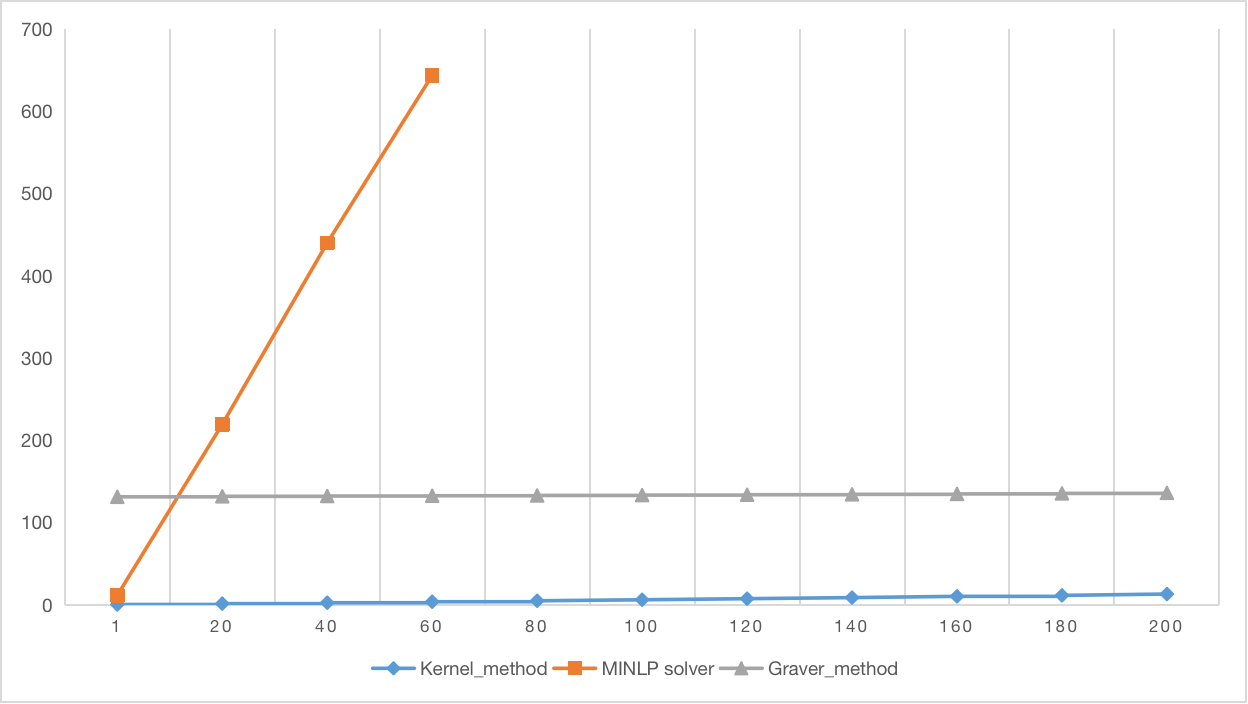
Figure 5.1. Trends of Computational Costs when the Sub-problem is Fixed

Figure 5.1 shows that Algorithm 4 took almost 130 seconds to initialize and then the curve rises slowly. The computational cost of the MINLP solver grows extremely fast and starts to overpower the Algorithm 4 when $N=20$. Generally, the curve of Algorithm 3 shows superior performance when compared with the other two algorithms.

Next, we compare when the complexity of the sub-problems increases. Below is the graph showing the trends of computational costs when the size of scenarios is fixed to 200 but the number of scenarios is increased. In Figure 5.2, with a fixed 200 scenarios, var*$x$ represents $x$ variables in the particular programming problem. As can be seen, by comparing the curves, the Gröbner Basis approach (the blue curve) is overall superior to the Graver Basis approach (the grey curve) and the traditional MINLP solver (the yellow curve). Also, regarding details, the Graver Basis method begins to suffer from the curse of dimensionality, starting from the problem’s complexity being 20 variables, and so is the Gröbner Basis method but more dramatically. However, the MINLP solver does not reflect the apparent complexity when it suffers from the curse. Generally, the MINLP solver applies to situations where the sub-problem is large, and the number of scenarios is small. In contrast, the Gröbner Basis applies to situations where the sub-problem has little complexity, and the number of scenarios is significant.

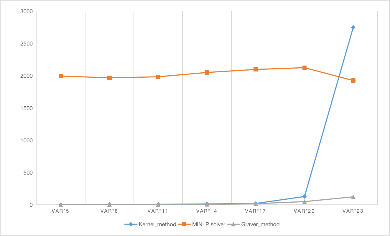
Figure 5.2. Trends of Computational Costs when the Quantity of Scenarios is Fixed

We have yet to reflect one thing in the experiments. By testing our algorithm hundreds of times, we have come to the empirical conclusion that the time increase of our proposed algorithm in computing Grobner Basis will be dramatic for $N>15$. And there will be geometric growth for the computational time regarding Graver Basis when the complexity is between 10 and 15 variables. Also, surprisingly, we can no longer compute the Gröbner Basis after 15 variables’ complexity. We refer to this phenomenon as the curse of dimensionality in computational algebraic geometry regarding SIP problems. We conjecture that the crux is that the number of ideal minimal generating elements will increase dramatically as the dimension increases, thus making Bunchberger’s algorithm computationally costly.

Finally, the crux of the problem, that two algebraic methods don’t function when the variables’ number exceeds 15, is the computation of the Gröbner Basis of some specific ideals, specifically the toric ideal of the coefficient matrix $A$, unavoidable in each of the two algorithms. We have tried many applications specialized in algebraic calculations, for example, SageMath, Macaulay2, etc. Still, when the variables’ number exceeds 15, usually the exponential of the generating elements of the polynomial ideal, which is required in the algorithm, is too great to be computable. For example, the computation of the Gröbner Basis of the matrix $A=(B,I)$ where $I$ denotes the identity matrix and

$$B=\begin{pmatrix}1&1&1&1&1&1&1&1&1&1\\ 1&2&3&4&5&6&7&8&9&10\\ 2&3&4&5&6&7&8&9&10&11\\ 3&4&5&6&7&8&9&10&11&12\\ 4&5&6&7&8&9&10&11&12&13\\ 5&6&7&8&9&10&11&12&13&14\\ 6&7&8&9&10&11&12&13&14&15\\ \end{pmatrix}$$

involves the computation of the Gröbner Basis of the toric ideal below

$\text{ideal}(x_{8}^{2}-x_{7}*x_{9}, x_{7}*x_{8}-x_{6}*x_{9},x_{6}*x_{8}-x_{5}*x_{9},x_{5}*x_{8}-x_{4}*x_{9},x_{4}*x_{8}-x_{3}*x_{9}, x_{3}*x_{8}-x_{2}*x_{9}, x_{2}*x_{8}-x_{1}*x_{9}, x_{1}*x_{8}-x_{0}*x_{9}, x_{7}^{2}-x_{5}*x_{9}, x_{6}*x_{7}-x_{4}*x_{9},x_{5}*x_{7}-x_{3}*x_{9},x_{4}*x_{7}-x_{2}*x_{9},x_{3}*x_{7}-x_{1}*x_{9}, x_{2}*x_{7}-x_{0}*x_{9}, x_{1}*x_{7}-x_{0}*x_{8},x_{6}^{2}-x_{3}*x_{9}, x_{5}*x_{6}-x_{2}*x_{9},x_{4}*x_{6}-x_{1}*x_{9},x_{3}*x_{6}-x_{0}*x_{9},x_{2}*x_{6}-x_{0}*x_{8}, x_{1}*x_{6}-x_{0}*x_{7}, x_{5}^{2}-x_{1}*x_{9}, x_{4}*x_{5}-x_{0}*x_{9},x_{3}*x_{5}-x_{0}*x_{8},x_{2}*x_{5}-x_{0}*x_{7},x_{1}*x_{5}-x_{0}*x_{6},x_{4}^{2}-x_{0}*x_{8}, x_{3}*x_{4}-x_{0}*x_{7},x_{2}*x_{4}-x_{0}*x_{6},x_{1}*x_{4}-x_{0}*x_{5},x_{3}^{2}-x_{0}*x_{6}, x_{2}*x_{3}-x_{0}*x_{5},x_{1}*x_{3}-x_{0}*x_{4},x_{2}^{2}-x_{0}*x_{4}, x_{1}*x_{2}-x_{0}*x_{3},x_{1}^{2}-x_{0}*x_{2}, x_{8}*x_{11}*x_{12}*x_{13}*x_{14}*x_{15}*x_{16}-x_{9},x_{7}*x_{11}*x_{12}*x_{13}*x_{14}*x_{15}*x_{16}-x_{8},x_{6}*x_{11}*x_{12}*x_{13}*x_{14}*x_{15}*x_{16}-x_{7},x_{5}*x_{11}*x_{12}*x_{13}*x_{14}*x_{15}*x_{16}-x_{6},x_{4}*x_{11}*x_{12}*x_{13}*x_{14}*x_{15}*x_{16}-x_{5},x_{3}*x_{11}*x_{12}*x_{13}*x_{14}*x_{15}*x_{16}-x_{4},x_{2}*x_{11}*x_{12}*x_{13}*x_{14}*x_{15}*x_{16}-x_{3},x_{1}*x_{11}*x_{12}*x_{13}*x_{14}*x_{15}*x_{16}-x_{2},x_{0}*x_{11}*x_{12}*x_{13}*x_{14}*x_{15}*x_{16}-x_{1},x_{9}*x_{10}*x_{14}*x_{15}^{2}*x_{16}^{3}-x_{0}*x_{6}*x_{11}^{2}* x_{12},x_{8}*x_{10}*x_{14}*x_{15}^{2}*x_{16}^{3}-x_{0}*x_{5}*x_{11}^{2}* x_{12},x_{7}*x_{10}*x_{14}*x_{15}^{2}*x_{16}^{3}-x_{0}*x_{4}*x_{11}^{2}* x_{12},x_{6}*x_{10}*x_{14}*x_{15}^{2}*x_{16}^{3}-x_{0}*x_{3}*x_{11}^{2}* x_{12},x_{5}*x_{10}*x_{14}*x_{15}^{2}*x_{16}^{3}-x_{0}*x_{2}*x_{11}^{2}* x_{12},x_{4}*x_{10}*x_{14}*x_{15}^{2}*x_{16}^{3}-x_{0}*x_{1}*x_{11}^{2}* x_{12},x_{3}*x_{10}*x_{14}*x_{15}^{2}*x_{16}^{3}-x_{0}^{2}*x_{11}^{2}* x_{12},x_{0}*x_{5}*x_{11}^{3}*x_{12}^{2}*x_{13}-x_{9}*x_{10}*x_{15}*x_{16}^{2},x_{0}*x_{4}*x_{11}^{3}*x_{12}^{2}*x_{13}-x_{8}*x_{10}*x_{15}*x_{16}^{2},x_{0}*x_{3}*x_{11}^{3}*x_{12}^{2}*x_{13}-x_{7}*x_{10}*x_{15}*x_{16}^{2},x_{0}*x_{2}*x_{11}^{3}*x_{12}^{2}*x_{13}-x_{6}*x_{10}*x_{15}*x_{16}^{2},x_{0}*x_{1}*x_{11}^{3}*x_{12}^{2}*x_{13}-x_{5}*x_{10}*x_{15}*x_{16}^{2},x_{0}^{2}*x_{11}^{3}*x_{12}^{2}*x_{13}-x_{4}*x_{10}*x_{15}*x_{16}^{2},x_{2}*x_{10}*x_{13}*x_{14}^{2}*x_{15}^{3}*x_{16}^{4}-x_{0}^{2}*x_{11},x_{1}*x_{10}*x_{12}*x_{13}^{2}*x_{14}^{3}*x_{15}^{4}*x_{16}^{5}-x_{0}^{2},x_{10}*x_{11}*x_{12}^{2}*x_{13}^{3}*x_{14}^{4}*x_{15}^{5}*x_{16}^{6}-x_{0}),$

In future work, we will study how the situation can be improved by optimising the algorithm for computation of Gröbner bases, for example, the Faugère $F_{4}$ [9] and $F_{5}$ [10] algorithms.

5.2. Stochastic network design

We have also tested our approach on a small stochastic network design problem, formulated as follows:

(5.4) $$\min \sum_{a\in A}c_{a}x_{a}+\frac{1}{N}\sum_{i=1}^{N}\sum_{c\in C}\sum_{a\in A}q_{ac}y_{ac}^{i}$$

(5.5) s.t. $$\sum_{\begin{subarray}{c}a\in A\\ a(0)=v\end{subarray}}y_{ac}^{i}-\sum_{\begin{subarray}{c}a\in A\\ a(1)=v\end{subarray}}y_{ac}^{i}=d_{v,c}^{i}\quad\forall(v,c,i)\in V\times C\times\{1,\ldots,N\}$$

(5.6) $$\sum_{c\in C}y_{ac}^{i}\leq u_{a}x_{a}\quad\forall(a,i)\in A\times\{1,\ldots,N\}$$

(5.7) $$x_{a}\in\{0,1\},y_{ac}^{i}\in\mathbb{Z}_{\geq 0}$$

Following the same procedure as in Section 5.1, we compare our two algorithms with a commercial solver. Our instances concern a small problem, with three vertices and three arcs. Figure 5.3 shows the time taken to compute the opportunity cost matrix for each approach.

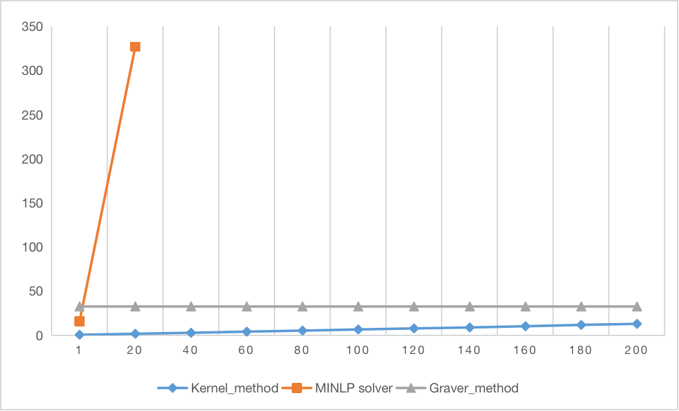
Figure 5.3. Trends of Computational Costs when the Sub-problem is Fixed (Stochastic Network Design Problem)

We once more observe the superior efficiency of the kernel approach when the number of decision variables is small.

6. Conclusion

In this paper, we have presented new algorithms for computing the opportunity cost matrix of [15] using algebraic methods using Gröbner and Graver bases. We have also provided mathematical results showing the relationship of Graver bases for deterministic and stochastic integer programs. Our numerical results show that the Gröbner basis is very efficient as the number of scenarios increases if the number of variables of the underlying integer program does not grow too fast. On the other hand, the Graver basis approach is interesting when there are a large number of variables.

In future work, we propose to include more recent methods of computing Gröbner basis, such as the Faugère algorithms. We will also study how to combine the algebraic approach with approximations such as Lagrangian cuts in order to increase further the number of decision variables that our approach can handle.

References

- [1] Dimitris Bertsimas and Nishanth Mundru “Optimization-Based Scenario Reduction for Data-Driven Two-Stage Stochastic Optimization” In Operations Research, 2022 DOI: 10.1287/opre.2022.2265
- [2] Dimitris Bertsimas, Georgia Perakis and Sridhar Tayur “A New Algebraic Geometry Algorithm for Integer Programming” In Management Science 46, 2000, pp. 999–1008 DOI: 10.1287/mnsc.46.7.999.12033
- [3] Fausto Di Biase and Rüdiger Urbanke “An Algorithm to Calculate the Kernel of Certain Polynomial Ring Homomorphisms” In Experimental Mathematics 4, 1995, pp. 227–234 DOI: 10.1080/10586458.1995.10504323
- [4] John R. Birge and François Louveaux “Introduction to Stochastic Programming” Springer New York, 2011 DOI: 10.1007/978-1-4614-0237-4
- [5] Bruno Buchberger “Gröbner Bases: An Algorithmic Method in Polynomial Ideal Theory” In Multidimensional Systems Theory and Applications D. Riedel Publications, 1985 DOI: 10.1007/978-94-017-0275-1˙4
- [6] Pasqualina Conti and Carlo Traverso “Buchberger algorithm and integer programming” In Applied Algebra, Algebraic Algorithms and Error-Correcting Codes Springer, 1991, pp. 130–139 DOI: 10.1007/3-540-54522-0˙102
- [7] David A. Cox, John Little and Donal O’Shea “Ideals, Varieties, and Algorithms” Springer International Publishing, 2015 DOI: 10.1007/978-3-319-16721-3
- [8] Jitka Dupacová, Nicole Gröwe-Kuska and Werner Römisch “Scenario reduction in stochastic programming” In Mathematical Programming 95, 2003, pp. 493–511 DOI: 10.1007/s10107-002-0331-0
- [9] Jean-Charles Faugère “A new efficient algorithm for computing Gröbner bases (F4)” In Journal of Pure and Applied Algebra 139, 1999, pp. 61–88 DOI: 10.1016/S0022-4049(99)00005-5
- [10] Jean-Charles Faugère “A new efficient algorithm for computing Gröbner bases without reduction to zero (F5)” In Proceedings of the 2002 international symposium on Symbolic and algebraic computation ACM, 2002, pp. 75–83 DOI: 10.1145/780506.780516
- [11] Jack E. Graver “On the foundations of linear and integer linear programming I” In Mathematical Programming 9, 1975, pp. 207–226 DOI: 10.1007/BF01681344
- [12] Raymond Hemmecke “On the positive sum property and the computation of Graver test sets” In Mathematical Programming 96, 2003, pp. 247–269 DOI: 10.1007/s10107-003-0385-7
- [13] Raymond Hemmecke and Rüdiger Schultz “Decomposition of test sets in stochastic integer programming” In Mathematical Programming 94 Springer ScienceBusiness Media LLC, 2003, pp. 323–341 DOI: 10.1007/s10107-002-0322-1
- [14] René Henrion, Christian Küchler and Werner Römisch “Scenario reduction in stochastic programming with respect to discrepancy distances” In Computational Optimization and Applications 43, 2009, pp. 67–93 DOI: 10.1007/s10589-007-9123-z
- [15] Mike Hewitt, Janosch Ortmann and Walter Rei “Decision-based scenario clustering for decision-making under uncertainty” In Annals of Operations Research 315 Springer, 2022, pp. 747–771 DOI: 10.1007/s10479-020-03843-x
- [16] Julien Keutchayan, Janosch Ortmann and Walter Rei “Problem-Driven Scenario Clustering in Stochastic Optimization”, 2021
- [17] Anton J. Kleywegt, Alexander Shapiro and Tito Homem Mello “The Sample Average Approximation Method for Stochastic Discrete Optimization” In SIAM Journal on Optimization 12, 2002, pp. 479–502 DOI: 10.1137/S1052623499363220
- [18] Werner Römisch “Scenario Reduction Techniques in Stochastic Programming” In Stochastic Algorithms: Foundations and Applications. SAGA 2009. Lecture Notes in Computer Science 5792, 2009, pp. 1–14 DOI: 10.1007/978-3-642-04944-6˙1
- [19] Rüdiger Schultz “On structure and stability in stochastic programs with random technology matrix and complete integer recourse” In Mathematical Programming 70, 1995, pp. 73–89
- [20] Rüdiger Schultz, Leen Stougie and Maarten H. Vlerk “Solving stochastic programs with integer recourse by enumeration: A framework using Gröbner basis” In Mathematical Programming 83, 1998, pp. 229–252 DOI: 10.1007/BF02680560
- [21] Bernd Sturmfels “Algebraic Recipes for Integer Programming” In Proceedings of Symposia in Applied Mathematics vo. 61, 2004, pp. 99–113
- [22] Bernd Sturmfels “Grobner bases and convex polytopes” American Mathematical Society, 1996
- [23] Rekha R. Thomas “Gröbner Bases in Integer Programming” In Handbook of Combinatorial Optimization Springer US, 1998, pp. 533–572 DOI: 10.1007/978-1-4613-0303-9˙8
- [24] R.R. Thomas and R. Weismantel “Truncated Gröbner bases for integer programming” In Applicable Algebra in Engineering, Communications and Computing 8, 1997, pp. 241–256 DOI: 10.1007/s002000050062