Transversal motion planning

Abstract.

In this paper, we introduce the notion of transversal topological complexity (TTC) for a smooth manifold $X$ with respect to a submanifold of codimension 1 together with basic results about this numerical invariant. In addition, we present several examples of explicit transversal algorithms.

1. Introduction

Let $X$ be the space of all possible obstacle-free configurations or states of a given autonomous system. A motion planning algorithm on $X$ is a function which, to any pair of configurations $(C_{1},C_{2})\in X\times X$, assigns a continuous motion $\mu$ of the system, so that $\mu$ starts at the given initial state $C_{1}$ and ends at the final desired state $C_{2}$. The fundamental problem in robotics, the motion planning problem, deals with how to provide, to any given autonomous system, with a motion planning algorithm.

For practical purposes, a motion planning algorithm should depend continuously on the pair of points $(C_{1},C_{2})$. Indeed, if the autonomous system performs within a noisy environment, absence of continuity could lead to instability issues in the behavior of the motion planning algorithm. Unfortunately, a (global) continuous motion planning algorithm on a space $X$ exists if and only if $X$ is contractible. Yet, if $X$ is not contractible, we could care about finding local continuous motion planning algorithms, i.e., motion planning algorithms $s$ defined only on a certain open subset of $X\times X$, to which we refer as the domain of definition of $s$. In these terms, a motion planner on $X$ is a set of local continuous motion planning algorithms whose domains of definition cover $X\times X$. The topological complexity of $X$ [2], TC$(X)$, is then the minimal cardinality among motion planners on $X$, while a motion planner on $X$ is said to be optimal if its cardinality is TC$(X)$. The design of explicit motion planners that are reasonably close to optimal is one of the challenges of modern robotics (see, for example Latombe [4] and LaValle [5]).

In more detail, the components of the motion planning problem via topological complexity are as follows (see [7]):

Formulation 1.1.

Ingredients in the motion planning problem via topological complexity:

1. The obstacle-free configuration space $X$. The topology of this space is assumed to be fully understood in advance.

2. Query pairs $C=(C_{1},C_{2})\in X\times X$. The point $C_{1}{}\in X$ is designated as the initial configuration of the query. The point $C_{2}{}\in X$ is designated as the goal configuration.

In the above setting, the goal is to either describe a motion planner, i.e., describe

1. An open covering $U=\{U_{1},\ldots,U_{k}\}$ of $X\times X$;

2. For each $i\in\{1,\ldots,k\}$, a local continuous motion planning algorithm, i.e., a continuous map $s_{i}\colon U_{i}\to X^{[0,1]}$ satisfying

   $$s_{i}(C)\left(j\right)=C_{j+1},\quad j=0,1$$

   for any $C=(C_{1},C_{2}){}\in U_{i}$ (here $X^{[0,1]}$ stands for the free-path space on $X$ joint with the compact-open topology),

or, else, report that such an planner does not exist.

Let $X$ be a smooth manifold and $Z\subset X$ be a submanifold with codimension $1$.

Definition 1.2.

A path $\Gamma:[0,1]\to X$ is semi-transversal to $Z$, denoted by $\Gamma\pitchfork_{s}Z$, if $\Gamma(t)\in Z$ with $t\in(0,1)$, implies that $\Gamma$ is smooth in $t$ and $\langle\Gamma^{\prime}(t)\rangle+T_{\Gamma(t)}Z=T_{\Gamma(t)}X$ (equivalently, $\Gamma^{\prime}(t)\notin T_{\Gamma(t)}Z$), where $\langle\Gamma^{\prime}(t)\rangle$ is the subspace generated by $\Gamma^{\prime}(t)$. Note that, if $\Gamma$ is transversal to $Z$ (we will denote $\Gamma\pitchfork Z$) then $\Gamma\pitchfork_{s}Z$.

Example 1.3.

The path $\Gamma\colon[0,1]\to\mathbb{R}^{2}$ given by

$$\Gamma(t)=\begin{cases}(1-2t)(-1,0)+2t(0,1),&\hbox{for $0\leq t\leq 1/2$;}\\ (2-2t)(0,1)+(1-2t)(1,0),&\hbox{for $1/2\leq t\leq 1$;}\end{cases}$$

is semi-transversal to $Z=\{(x,x):~{}x\in\mathbb{R}\}$ but is not transversal to $Z$. In fact, $\Gamma$ is not smooth in $t=1/2$.

Investigation of the problem of transversal motion planners for a robot, with state space $X$, leads us to study the pair $(X,Z)$, where $Z$ is a submanifold of $X$ with codimension $1$. The submanifold $Z$ may characterize some desired geometry for the motion planning algorithm. A (local) transversal motion planning algorithm in $X$ with respect to $Z$ assigns to any pair of configurations $(C_{1},C_{2})$ in (an open set of) $X\times X$ a path of configurations

$$\Gamma(t)\in X,~{}~{}t\in[0,1],$$

such that $\Gamma\left(i\right)=C_{i+1}$ for $i=0,1$ and $\Gamma\pitchfork_{s}Z$.

In this work we introduce the notion of transversal topological complexity together with basic results about this numerical invariant. Proposition 2.3 together with Example 2.4 give the motivation to introduce the tranversal topological complexity (Definition 2.5). Examples 2.7 and 2.8 present transversal algorithms in euclidean spaces. We define the notion of transversal LS category (Definition 2.10) and present a lower bound for transversal complexity in terms of transversal LS category (Proposition 2.12). Proposition 2.15 shows an explicit construction of transversal algorithms through diffeomorphisms. Examples 2.13 and 2.16 show that submanifold $Z$ may imply some desired geometry for the motion planning algorithm.

2. Transversal topological complexity

In this section we present the notion of transversal topological complexity (Definition 2.5) together with basic results about this numerical invariant (Lemma 2.9 and Propositions 2.12 and 2.15). Several examples are presented to illustrate the result arising in this field (Examples 2.7, 2.8, 2.13 and 2.16). Examples 2.13 and 2.16 show that submanifold $Z$ may imply some desired geometry for the motion planning algorithm.

Let $X^{[0,1]}$ stand for the free-path space of a topological space $X$. Recall that Farber’s topological complexity $\text{TC}(X)$ is the sectional category of the end-points evaluation fibration $e_{2}^{X}\colon X^{[0,1]}\to X\times X$, $e_{2}^{X}(\gamma)=(\gamma(0),\gamma(1))$. We use sectional category of a fibration $p\colon E\to B$ in the non reduced sense, i.e., it is the minimal number of open sets covering $B$ and on each of which $p$ admits a local continuous section.

From the Whitney approximation theorem [6, Theorem 6.26] we obtain the following statement.

Lemma 2.1.

Let $X$ and $Y$ be smooth manifolds (without boundary), $f,g:X\to Y$ be smooth maps such that there is a continuous homotopy $H:X\times[0,1]\to Y$ with $H_{0}=f$ and $H_{1}=g$, then there exists a smooth homotopy $G:X\times[0,1]\to Y$ with $G_{0}=f$ and $G_{1}=g$.

From [3, Pg. 73] we have the following statement.

Lemma 2.2.

Let $f:X\to Y$ be a smooth map and $Z\subset Y$ be a submanifold such that the boundary map $\partial f:\partial X\to Y$ is transversal to $Z$, then there exists a smooth map $g:X\to Y$ homotopic to $f$ such that $\partial g=\partial f$ and $g\pitchfork Z$.

Then, we have the following statement

Proposition 2.3.

Let $X$ be a smooth manifold and $Z\subset X$ be a submanifold of codimension $1$, then $\text{TC}(X)$ coincides with the smallest positive integer $k$ for which the product $X\times X$ is covered by $k$ open subsets $X\times X=U_{1}\cup\cdots\cup U_{k}$ such that for any $i=1,2,\ldots,k$ there exists a continuous section $s_{i}:U_{i}\to X^{[0,1]}$ of $e_{2}^{X}$ over $U_{i}$ (i.e., $e_{2}^{X}\circ s_{i}=incl_{U_{i}}$) and $\widetilde{s_{i}}\pitchfork Z$, where $\widetilde{s_{i}}\colon U_{i}\times[0,1]\to X$ is given by $\widetilde{s_{i}}(u)=s_{i}(u)(t)$ for any $u\in U_{i}$ and $t\in[0,1]$.

Proof.

For $U\subset X\times X$ and $s:U\to X^{[0,1]}$ a continuous local algorithm, consider $\widetilde{s}:U\times[0,1]\to X,~{}\widetilde{s}((x,y),t)=s(x,y)(t)$. Note that, $\widetilde{s}$ is a continuos homotopy with $\widetilde{s}_{0}=\pi_{1}$ and $\widetilde{s}_{1}=\pi_{2}$, where $\pi_{j}$ is the projection to the $j$-th factor. By Lemma 2.1, there exists a smooth homotopy $G:U\times[0,1]\to X$ with $G_{0}=\pi_{1}$ and $G_{1}=\pi_{2}$. Note that the boundary map $\partial G=\pi_{1}\sqcup\pi_{2}$ is transversal to $Z$, then by Lemma 2.2, there exists a smooth map $F:U\times[0,1]\to X$ homotopic to $G$ such that $\partial F=\partial G$ (and thus, $F_{0}=\pi_{1}$ and $F_{1}=\pi_{2}$) and $F\pitchfork Z$. Then, the map $\sigma\colon U\to X^{[0,1]}$ given by $\sigma(x,y)(t)=F((x,y),t)$ satisfies the conditions of the proposition. Thus, the proposition holds. ∎

Note that, if $F:U\times[0,1]\to X$ is transversal to $Z$ with $U\subset X\times X$ does not implies that $F_{u}\colon[0,1]\to X,~{}t\mapsto F_{u}(t)=F(u,t)$, is transversal to $Z$ for any $u\in U$. To see this, we have the following example.

Example 2.4.

Consider the pair $\left(\mathbb{R}^{2},S^{1}\right)$ and the smooth map $F\colon\mathbb{R}^{2}\times\mathbb{R}^{2}\times[0,1]\to\mathbb{R}^{2}$ given by $F\left((C_{1},C_{2}),t\right)=(1-t)C_{1}+tC_{2}$. Note that, $F\pitchfork S^{1}$ but $F_{\left((1,1),(-1,1)\right)}\colon[0,1]\to\mathbb{R}^{2},~{}F_{\left((1,1),(-1,1)\right)}(t)=\left(1-2t,1\right)$, is not transversal to $S^{1}$.

Proposition 2.3 says that Farber’s topological complexity of $X$ coincides with the complexity of designing smooth homotopies $F:U\times[0,1]\to X$ with $F_{0}=\pi_{1}$ and $F_{1}=\pi_{2}$ such that $F\pitchfork Z$. However, Example 2.4 motives the following definition.

Definition 2.5.

The transversal topological complexity TTC$(X,Z)$ of a path-connected smooth manifold (without boundary) $X$ with respect to a submanifold (without boundary) $Z$ with codimension 1 is the smallest positive integer TTC$(X,Z)=k$ for which the product $X\times X$ is covered by $k$ open subsets $X\times X=U_{1}\cup\cdots\cup U_{k}$ such that for any $i=1,2,\ldots,k$ there exists a continuous section $s_{i}:U_{i}\to X^{[0,1]}$ of $e_{2}^{X}$ over $U_{i}$ (i.e., $e_{2}^{X}\circ s_{i}=incl_{U_{i}}$) and $s_{i}(x,y)\pitchfork_{s}Z$ for any $(x,y)\in U_{i}$. We call such a collection of local sections a transversal motion planner with $k$ domains of continuity. If no such $k$ exists, we set TTC$(X,Z)=\infty$.

Remark 2.6.

Note that $\text{TC}(X)\leq\text{TTC}(X,Z)$ for any smooth manifold $X$ and any submanifold $Z\subset X$ with codimension 1.

Example 2.7.

Consider the pair $(\mathbb{R}^{n},\mathbb{R}^{n-1})$, with the latter understood as the submanifold $\mathbb{R}^{n-1}\times\{0\}\subset\mathbb{R}^{n}$. We claim that the transversal topological complexity of this pair is 1. Indeed, consider the (global) algorithm $s:\mathbb{R}^{n}\times\mathbb{R}^{n}\to(\mathbb{R}^{n})^{[0,1]}$ defined by

$$s(C_{1},C_{2})(t)=\begin{cases}(1-2t)C_{1}+2te_{n},&\hbox{for $0\leq t\leq 1/2$;}\\ (2-2t)e_{n}+(2t-1)C_{2},&\hbox{for $1/2\leq t\leq 1$;}\\ \end{cases}$$

where $e_{n}=(0,\ldots,0,1)\in\mathbb{R}^{n}$. This map (see Figure 1) is continuous and satisfies the transversal condition: If $s(C_{1},C_{2})(t)\in\mathbb{R}^{n-1}$ with $t\in(0,1)$, then

$$s^{\prime}(C_{1},C_{2})(t)=\begin{cases}2(e_{n}-C_{1}),&\hbox{for $0<t<1/2$;}\\ 2(C_{2}-e_{n}),&\hbox{for $1/2<t<1$;}\\ \end{cases}$$

Hence, $s^{\prime}(C_{1},C_{2})(t)\notin\mathbb{R}^{n-1}$.

Figure 1. The transversal algorithm $s(C_{1},C_{2})(t)$ in $\mathbb{R}^{2}$ with respect to the 1-codimension submanifold $W=\{(a,0):~{}a\in\mathbb{R}\}$.

Example 2.8.

For the pair $\left(\mathbb{R}^{d+1},\bigsqcup_{i=1}^{n}S^{d}_{i}(0)\right)$ where $S^{d}_{i}(0)$ is the $d$-dimensional sphere with center $0$ and radius $i$, $i=1,\ldots,n$, then we have that the transversal topological complexity $\text{TTC}(\mathbb{R}^{d+1},\bigsqcup_{i=1}^{n}S^{d}_{i}(0))=1$. To check this, we have that the map $s:\mathbb{R}^{d+1}\times\mathbb{R}^{d+1}\to\left(\mathbb{R}^{d+1}\right)^{[0,1]}$ given by

$$s(C_{1},C_{2})(t)=\begin{cases}(1-2t)C_{1},&\hbox{for $0\leq t\leq 1/2$;}\\ (2t-1)C_{2},&\hbox{for $1/2\leq t\leq 1$;}\\ \end{cases}$$

defines a global continuous transversal algorithm in $\mathbb{R}^{d+1}$ with respect to $\bigsqcup_{i=1}^{n}S^{d}_{i}(0)$ (see Figure 2).

Figure 2. Global transversal algorithm in $\mathbb{R}^{d+1}$ with respect to $S^{d}_{1}(0)\sqcup S^{d}_{2}(0)$.

Let $X$ be a smooth manifold, $Z\subset X$ be a 1-codimension submanifold and $x_{0}\in X\setminus Z$. We have the following statement.

Lemma 2.9.

There exists a continuous transversal algorithm $s:X\times X\to X^{[0,1]}$ with respect to $Z$ if and only if there exists a continuous nulhomotopy $H:X\times[0,1]\to X$ with $H_{0}=1_{X}$, $H_{1}=\overline{x_{0}}$ and $H(x,-)\pitchfork_{s}Z$ for any $x\in X$.

Proof.

Suppose that $s:X\times X\to X^{[0,1]}$ is a continuous transversal algorithm with respect to $Z$. The map $H:X\times[0,1]\to X$ given by $H(x,t)=s(x,x_{0})(t)$ defines a continuous nulhomotopy with $H_{0}=1_{X}$, $H_{1}=\overline{x_{0}}$ and $H(x,-)\pitchfork_{s}Z$ for any $x\in X$.

Now, suppose that $H:X\times[0,1]\to X$ is a continuous nulhomotopy with $H_{0}=1_{X}$, $H_{1}=\overline{x_{0}}$ and $H(x,-)\pitchfork_{s}Z$ for any $x\in X$. The map $s:X\times X\to X^{[0,1]}$ given by

$$s(x,y)(t)=\begin{cases}H(x,2t),&\hbox{for $0\leq t\leq 1/2$;}\\ H(y,2-2t),&\hbox{for $1/2\leq t\leq 1$;}\\ \end{cases}$$

defines a continuous transversal algorithm with respect to $Z$ (here we use that $x_{0}\notin Z$). ∎

Lemma 2.9 implies the notion of transversal LS category.

Definition 2.10.

Let $X$ be a smooth manifold and $Z\subset X$ be a 1-codimension submanifold. The transversal LS category of $X$ with respect to $Z$, denoted by $\text{Tcat}(X,Z)$, is the smallest positive integer $k$ for which the space $X$ is covered by $k$ open subsets $X=U_{1}\cup\cdots\cup U_{k}$ such that for each $i=1,2,\ldots,k$ there exists a continuous map $H:U_{i}\times[0,1]\to X$ with $H_{0}=incl_{U_{i}}$, $H_{1}=constant$ and $H(x,-)\pitchfork_{s}Z$ for any $x\in U_{i}$. If no such $k$ exists, we set Tcat$(X,Z)=\infty$.

Note that $\text{Tcat}(X,Z)\geq\text{cat}(X)$, where $\text{cat}(X)$ is the LS category of $X$. From [1], the LS category of $X$ is the least integer $k$ such that $X$ can be covered by $k$ open sets, all of which are contractible within $X$.

Example 2.11.

Consider the pair $(\mathbb{R}^{2},S^{1}_{1}\sqcup S^{1}_{2})$, where $S^{1}_{1}$ is the $1$-sphere with center $O_{1}=(-2,0)$ and $S^{1}_{2}$ is the $1$-sphere with center $O_{2}=(2,0)$ (see Figure 3). We have that $\text{Tcat}(\mathbb{R}^{2},S^{1}_{1}\sqcup S^{1}_{2})=2$. We will prove $\text{Tcat}(\mathbb{R}^{2},S^{1}_{1}\sqcup S^{1}_{2})\leq 2$, the lower bound is a technical exercise which we leave to the reader. Consider the open sets:

$$U_{1} =\pi^{-1}\left(-\infty,1/2\right),$$

$$U_{2} =\pi^{-1}\left(-1/2,+\infty\right),$$

where $\pi:\mathbb{R}^{2}\to\mathbb{R}$ is the natural projection $\pi(x,y)=(x,0)$. Note that $U_{1}\cup U_{2}=\mathbb{R}^{2}$. Moreover, for each $i=1,2$, we can consider the map $H_{i}:U_{i}\times[0,1]\to\mathbb{R}^{2}$ given by

$$H_{i}(x,t) =(1-t)x+tO_{i}.$$

Note that $H_{i}(x,0)=x$, $H(x,1)=O_{i}$ and $H_{i}(x,-)\pitchfork_{s}S^{1}_{1}\sqcup S^{1}_{2}$ for any $x\in U_{i}$. Thus, $\text{Tcat}(\mathbb{R}^{2},S^{1}_{1}\sqcup S^{1}_{2})\leq 2$ and therefore $\text{Tcat}(\mathbb{R}^{2},S^{1}_{1}\sqcup S^{1}_{2})=2$.

Figure 3. The plane $\mathbb{R}^{2}$ with two disjoint copies of the $1$-dimensional sphere $S^{1}_{1}\sqcup S^{1}_{2}$.

The following statement presents a lower bound for transversal complexity in terms of transversal LS category.

Proposition 2.12.

Let $X$ be a smooth manifold and $Z\subset X$ be a 1-codimension submanifold. We have

$$\text{Tcat}(X,Z)\leq\text{TTC}(X,Z).$$

Proof.

Let $x_{0}\in X$ and consider the map $i_{0}\colon X\to X\times X$, $x\mapsto i_{0}(x)=(x,x_{0})$. For $U\subset X\times X$ and $s\colon U\to X^{[0,1]}$ satisfying $e_{2}^{X}\circ s=incl_{U}$ and $s(x,y)\pitchfork_{s}Z$ for any $(x,y)\in U$, consider $V=i_{0}^{-1}(U)$ and the map $H:V\times[0,1]\to X$ given by $H(x,t)=s(x,x_{0})(t)$ defines a continuous map with $H_{0}=incl_{V}$, $H_{1}=\overline{x_{0}}$ and $H(x,-)\pitchfork_{s}Z$ for any $x\in U$. Hence, we conclude that $\text{TTC}(X,Z)\geq\text{Tcat}(X,Z)$. ∎

Example 2.13.

Consider the pair $(\mathbb{R}^{2},S^{1}_{1}\sqcup S^{1}_{2})$, where $S^{1}_{1}$ is the $1$-sphere with center $(-2,0)$ and $S^{1}_{2}$ is the $1$-sphere with center $(2,0)$. We have that the transversal topological complexity $2\leq\text{TTC}(\mathbb{R}^{2},S^{1}_{1}\sqcup S^{1}_{2})\leq 4$. In fact, the first inequality follows from Example 2.11 together with Proposition 2.12. To check the second inequality, we can consider the open sets:

$$A =\bigcap_{i=1}^{4}\pi^{-1}\left(\mathbb{R}\setminus\{a_{i}\}\right),$$

$$B =\bigsqcup_{i=1}^{4}\pi^{-1}\left(a_{i}-1/4,a_{i}+1/4\right),$$

where $\pi:\mathbb{R}^{2}\to\mathbb{R}$ is the natural projection $\pi(x,y)=(x,0)$ and $a_{1}=(-3,0)$, $a_{2}=(-1,0)$, $a_{3}=(1,0)$ and $a_{4}=(2,0)$.

Note that $A\cup B=\mathbb{R}^{2}$ and thus $\left(A\times A\right)\cup\left(A\times B\right)\cup\left(B\times A\right)\cup\left(B\times B\right)=\mathbb{R}^{2}\times\mathbb{R}^{2}$. Moreover,

$$A\times B =\bigsqcup_{j=1}^{4}A\times\pi^{-1}\left(a_{j}-1/4,a_{j}+1/4\right),$$

$$B\times A =\bigsqcup_{i=1}^{4}\pi^{-1}\left(a_{i}-1/4,a_{i}+1/4\right)\times A,$$

$$B\times B =\bigsqcup_{i,j=1}^{4}\pi^{-1}\left(a_{i}-1/4,a_{i}+1/4\right)\times\pi^{-1}\left(a_{j}-1/4,a_{j}+1/4\right),$$

The following maps

$$s\colon A\times A\to\left(\mathbb{R}^{2}\right)^{[0,1]},$$

$$s_{A,j}\colon A\times\pi^{-1}\left(a_{j}-1/4,a_{j}+1/4\right)\to\left(\mathbb{R}^{2}\right)^{[0,1]},$$

$$s_{i,A}\colon \pi^{-1}\left(a_{i}-1/4,a_{i}+1/4\right)\times A\to\left(\mathbb{R}^{2}\right)^{[0,1]},$$

$$s_{i,j}\colon \pi^{-1}\left(a_{i}-1/4,a_{i}+1/4\right)\times\pi^{-1}\left(a_{j}-1/4,a_{j}+1/4\right)\to\left(\mathbb{R}^{2}\right)^{[0,1]},$$

given by

$$s(C_{1},C_{2})(t) =\begin{cases}(1-3t)C_{1}+3t\pi(C_{1}),&\hbox{ for $0\leq t\leq 1/3$;}\\ (2-3t)\pi(C_{1})+(3t-1)\pi(C_{2}),&\hbox{ for $1/3\leq t\leq 2/3$;}\\ (3-3t)\pi(C_{2})+(3t-2)C_{2},&\hbox{ for $2/3\leq t\leq 1$;}\\ \end{cases}$$

$$s_{A,j}(C_{1},C_{2})(t) =\begin{cases}(1-3t)C_{1}+3t\pi(C_{1}),&\hbox{ for $0\leq t\leq 1/3$;}\\ (2-3t)\pi(C_{1})+(3t-1)d_{j},&\hbox{ for $1/3\leq t\leq 2/3$;}\\ (3-3t)d_{j}+(3t-2)C_{2},&\hbox{ for $2/3\leq t\leq 1$;}\\ \end{cases}$$

$$s_{i,A}(C_{1},C_{2})(t) =\begin{cases}(1-3t)C_{1}+3td_{i},&\hbox{ for $0\leq t\leq 1/3$;}\\ (2-3t)d_{i}+(3t-1)\pi(C_{2}),&\hbox{ for $1/3\leq t\leq 2/3$;}\\ (3-3t)\pi(C_{2})+(3t-2)C_{2},&\hbox{ for $2/3\leq t\leq 1$;}\\ \end{cases}$$

$$s_{i,j}(C_{1},C_{2})(t) =\begin{cases}(1-3t)C_{1}+3td_{i},&\hbox{ for $0\leq t\leq 1/3$;}\\ (2-3t)d_{i}+(3t-1)d_{j},&\hbox{ for $1/3\leq t\leq 2/3$;}\\ (3-3t)d_{j}+(3t-2)C_{2},&\hbox{ for $2/3\leq t\leq 1$;}\\ \end{cases}$$

where $d_{1}=d_{2}=(-2,0)$ and $d_{3}=d_{4}=(2,0)$, define local continuous transversal algorithms with respect to $S^{1}_{1}\sqcup S^{1}_{2}$. We have thus constructed a transversal motion planner in $\mathbb{R}^{2}$ with respect to $S^{1}_{1}\sqcup S^{1}_{2}$ having $4$ regions of continuity $A\times A,A\times B,B\times A,B\times B$.

Figure 4. The local transversal algorithm $s\colon A\times A\to\left(\mathbb{R}^{2}\right)^{[0,1]}$.

Figure 5. The local transversal algorithm $s_{A,1}$.

Figure 6. The local transversal algorithm $s_{1,4}$.

The following result is technical.

Lemma 2.14.

Let $h:M\to N$ be a diffeomorphism. If $W\subset N$ is a submanifold with codimension $1$, then $Z=h^{-1}(W)\subset M$ is also a submanifold with codimension $1$.

Then, the next statement shows an explicit construction of transversal algorithms through diffeomorphisms.

Proposition 2.15.

Let $h\colon M\to N$ be a diffeomorphism. If $W\subset N$ is a submanifold with codimension $1$, then $\text{TTC}(N;W)=\text{TTC}(M;h^{-1}(W))$.

Proof.

Let $Z=h^{-1}(W)\subset M$. For $U\subset N\times N$ and $s\colon U\to N^{[0,1]}$ satisfying $e_{2}^{N}\circ s=incl_{U}$ and $s(x,y)\pitchfork_{s}W$ whenever $(x,y)\in U$, consider $V=\left(h\times h\right)^{-1}(U)\subset M\times M$, the map $\sigma\colon V\to M^{[0,1]}$ given by $\sigma=(h^{-1})_{\#}\circ s\circ\left(h\times h\right)_{\mid V}$ defines a local section of $e_{2}^{M}$, where $(h^{-1})_{\#}:N^{[0,1]}\to M^{[0,1]}$ is the induced map of $h^{-1}$, i.e., $(h^{-1})_{\#}(\alpha)=h^{-1}\circ\alpha$.

For any $(x,y)\in V$ we will show that $\sigma(x,y)\pitchfork_{s}Z$. First, note that $(h(x),h(y))\in U$ and thus $\Gamma=s(h(x),h(y))$ is such that $\Gamma\pitchfork_{s}W$. Also, note that $\sigma(x,y)=h^{-1}\circ\Gamma$ and $\sigma(x,y)(t)=h^{-1}\left(\Gamma(t)\right)$ for any $t\in[0,1]$. Suppose that $\sigma(x,y)(t_{0})\in Z$ for some $t_{0}\in(0,1)$, then $\Gamma(t_{0})\in W$ and so $\Gamma(t)$ is smooth for $t\in(0,1)$, and $\Gamma^{\prime}(t_{0})\notin T_{\Gamma(t_{0})}W$. Then $\sigma(x,y)(t)$ is smooth in $t_{0}\in(0,1)$ and $\sigma^{\prime}(x,y)(t_{0})=(dh^{-1})_{\Gamma(t_{0})}\left(\Gamma^{\prime}(t_{0})\right)\notin T_{\sigma(x,y)(t_{0})}Z$. Therefore, $\text{TTC}(N;W)\geq\text{TTC}(M;h^{-1}(W))$.

The inequality $\text{TTC}(M;h^{-1}(W))\geq\text{TTC}(N;W)$ follows from the first part applying to $h^{-1}\colon N\to M$ with $Z\subset M$. ∎

Example 2.16.

Consider the diffeomorphism $h\colon\mathbb{R}^{2}\to\mathbb{R}^{2},~{}h(x,y)=(x,y-x^{2})$, whose inverse $f\colon\mathbb{R}^{2}\to\mathbb{R}^{2}$ is given by $f(a,b)=(a,a^{2}+b)$. Set $W=\{(a,b)\in\mathbb{R}^{2}:~{}b=0\}$, then $Z=f(W)=\{(x,y)\in\mathbb{R}^{2}:~{}y=x^{2}\}$ is the parabola. From Example 2.7, we have that the map $s\colon\mathbb{R}^{2}\times\mathbb{R}^{2}\to\left(\mathbb{R}^{2}\right)^{[0,1]}$ given by

$$s(C_{1},C_{2})(t)=\begin{cases}(1-2t)C_{1}+2te_{2},&\hbox{for $0\leq t\leq 1/2$;}\\ (2-2t)e_{2}+(2t-1)C_{2},&\hbox{for $1/2\leq t\leq 1$;}\\ \end{cases}$$

where $e_{2}=(0,1)$, is a transversal continuous algorithm with respect to the submanifold $W$. Then, by Proposition 2.15, the map $\sigma\colon\mathbb{R}^{2}\times\mathbb{R}^{2}\to\left(\mathbb{R}^{2}\right)^{[0,1]}$ given by, for $B_{1}=(x_{1},y_{1})$ and $B_{2}=(x_{2},y_{2})$:

$$\sigma(B_{1},B_{2})(t) =f\left(s(h(B_{1}),h(B_{2}))(t)\right)$$

$$=\begin{cases}f\left((1-2t)h(B_{1})+2te_{2}\right),&\hbox{for $0\leq t\leq 1/2$;}\\ f\left((2-2t)e_{2}+(2t-1)h(B_{2})\right),&\hbox{for $1/2\leq t\leq 1$;}\\ \end{cases}$$

$$=\begin{cases}f\left((1-2t)(x_{1},y_{1}-x_{1}^{2})+2te_{2}\right),&\hbox{for $0\leq t\leq 1/2$;}\\ f\left((2-2t)e_{2}+(2t-1)(x_{2},y_{2}-x_{2}^{2})\right),&\hbox{for $1/2\leq t\leq 1$;}\\ \end{cases}$$

$$=\begin{cases}f\left((1-2t)x_{1},(1-2t)(y_{1}-x_{1}^{2})+2t\right),&\hbox{for $0\leq t\leq 1/2$;}\\ f\left((2t-1)x_{2},(2-2t)+(2t-1)(y_{2}-x_{2}^{2})\right),&\hbox{for $1/2\leq t\leq 1$;}\\ \end{cases}$$

$$=\begin{cases}\left((1-2t)x_{1},(1-2t)^{2}x_{1}^{2}+(1-2t)(y_{1}-x_{1}^{2})+2t\right),&\hbox{for $0\leq t\leq 1/2$;}\\ \left((2t-1)x_{2},(2t-1)^{2}x_{2}^{2}+(2-2t)+(2t-1)(y_{2}-x_{2}^{2})\right),&\hbox{for $1/2\leq t\leq 1$;}\\ \end{cases},$$

defines a transversal algorithm in $\mathbb{R}^{2}$ with respect to the parabola $Z$.

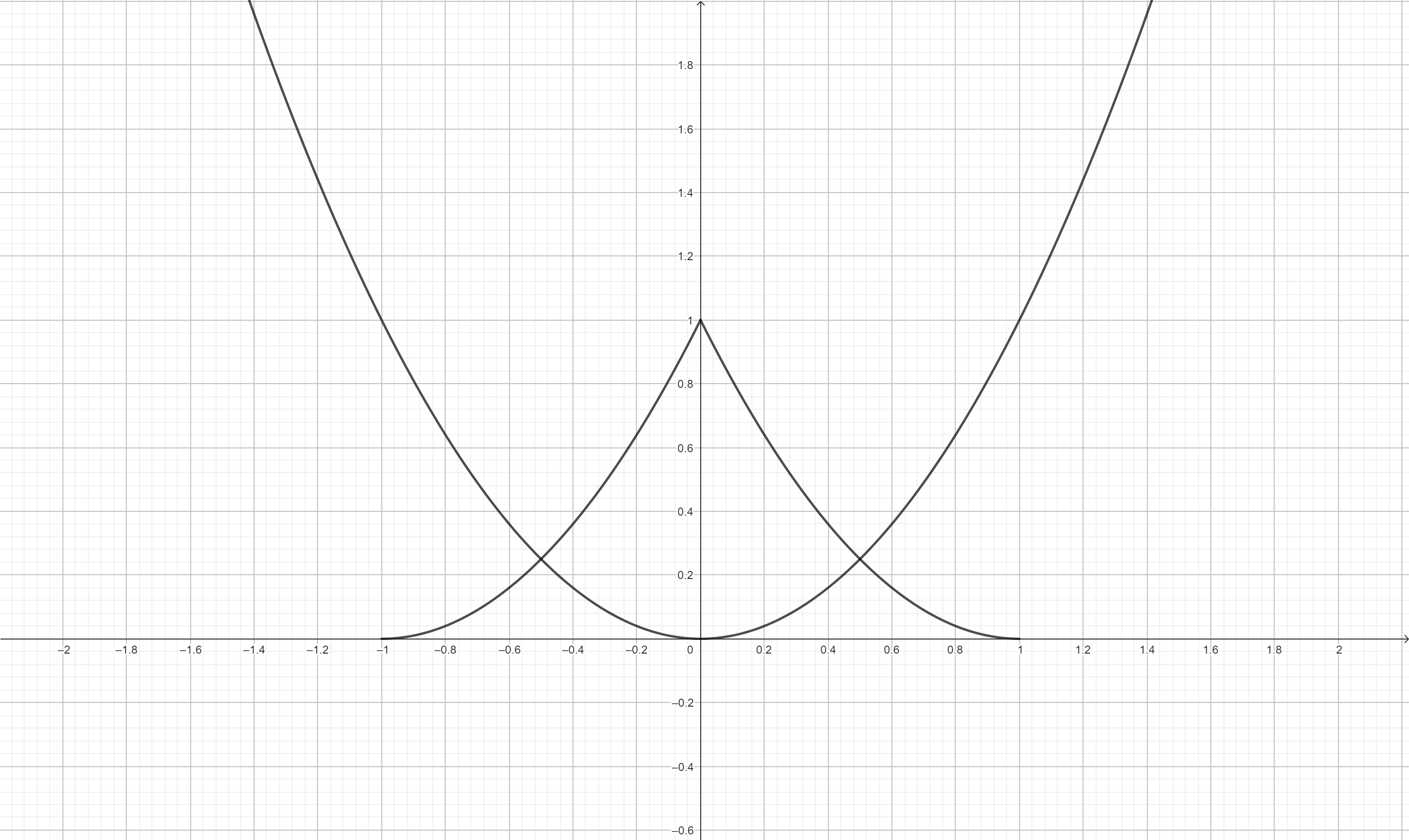
Figure 7. For $B_{1}=(-1,0)$ and $B_{2}=(1,0)$, the route given by the transversal algorithm $\sigma$ is $\sigma(B_{1},B_{2})(t)=\left(-(1-2t),(1-2t)^{2}+4t-1\right)$ for $0\leq t\leq 1/2$ and $\sigma(B_{1},B_{2})(t)=\left(2t-1,(2t-1)^{2}-4t+3\right)$ for $1/2\leq t\leq 1$.

References

- [1] O. Cornea, G. Lupton, J. Oprea and D. Tanré, ‘Lusternik-Schnirelmann Category’, Mathematical Surveys and Monographs, 103 (American Mathematical Society, Providence, RI, 2003).
- [2] M. Farber, Topological complexity of motion planning. Discrete and Computational Geometry. 29 (2003), no. 2, 211–221.
- [3] V. Guillemin and Al. Pollack. Differential topology. Vol. 370. American Mathematical Soc., 2010.
- [4] J. C. Latombe, Robot motion planning. Springer, New York (1991).
- [5] S. M. LaValle, Planning algorithms. Cambridge University Press, Cambridge. (2006).
- [6] J. Lee, Introduction to smooth manifolds. springer, 2012.
- [7] C. A. I. Zapata and J. Gonzalez, Multitasking collision-free optimal motion planning algorithms in Euclidean spaces. Discrete Mathematics, Algorithms and Applications, 12, no. 3 (2020) 2050040. doi:10.1142/S1793830920500408