Improved refrigeration in presence of non-Markovian spin-environment

Abstract

We explore a small quantum refrigerator consisting of three qubits each of which are kept in contact with an environment. We consider two settings: one is when there is necessarily transient cooling and the other is when both steady-state and transient cooling prevail. We show that there can be significant advantages than the Markovian environments case for both these settings in the transient regime and also in equilibrium if we replace the bath attached to the cold qubit by a non-Markovian reservoir. We also consider refrigeration with more than one non-Markovian bath of the three-qubit refrigerating device. Curiously, a steady temperature is reached only if there are at least two Markovian environments, although there are distinct envelopes of the temperature oscillations in all cases. We compare the device connected to one or more non-Markovian reservoirs with the case of all Markovian environs, as also with two- and single-qubit self-sustained devices connected to one or more non-Markovian baths. We propose a measure to quantify the amount of non-Markovianity in the systems. Finally, the refrigerator models are studied in presence of Markovian noise, and we analyse the response on the refrigeration of the noise strength. In particular, we find the noise strength until which refrigeration remains possible.

I Introduction

The onset and flourishing of quantum thermodynamics Allahverdyan ; Gemmer ; Kosloff ; Brand ; Gardas ; Gelbwaser ; Misra ; Millen ; Vinjanampathy ; Goold ; Benenti ; Binder ; Deffner has sustained the arena of quantum thermal devices, which in turn has gained utmost importance in the advancement of quantum technologies and in particular, for the miniaturisation of quantum circuits. In the last few decades, the achievement in designing quantum heat engines and quantum refrigerators Palao ; Feldmann ; Popescu ; Levy1 ; Levy ; Uzdin ; Clivaz ; Mitchison ; Scarani , quantum diodes Yuan , quantum thermal transistors Joulain ; Zhang ; Su ; Mandarino , quantum batteries Alicki_Fannes ; Campaioli ; Dutta has built the backbone of quantum technologies, which aims to enhance the efficiencies of quantum devices over their classical counterparts Kosloff2 ; Kosloff1 ; Wehner_new ; Kurizki_new ; Chen_Liu . The confluence of quantum thermodynamics with many-body physics Dorner ; Mehboudi ; Reimann ; Eisert ; Gogolin ; Skelt , quantum information theory Gour ; Vinjanampathy ; Goold , statistical and solid-state physics Fazio ; Rigol have triggered the implementations of quantum devices in experiments using superconducting qubits Pekola2 ; Aslan ; Jordan , mesoscopic substrates Pekola , ionic systems ionic1 ; ionic2 , nuclear magnetic resonance n_m_resonance , etc. The performance of such devices is evidently controlled by thermal baths or environments connected to the machinery setup, and the dynamics of the device components are driven by the open quantum evolutions Petruccione ; Alicki ; Rivas ; Lidar . The thermal baths, that influence the efficiency of performance of the devices, can either be Markovian or non-Markovian depending on the validity of Born-Markov approximations Petruccione ; Alicki ; Rivas ; Lidar . In general, the efficiencies of quantum thermal devices immersed in Markovian Petruccione environments are computable and the dynamics of the machinery components can be efficiently handled. Most of the thermal baths, however, reside in a non-Markovian family and therefore makes the realistic situations different from the ideal Markovian dynamics. There exists a significant body of work on quantum thermal machines operating under more than one thermal baths, which are either all Markovian Palao ; Levy1 ; Uzdin ; Mitchison ; Joulain ; Su ; Mandarino ; Dutta or all non-Markovian Dutta ; non-Markov ; Kurizki ; Uzdin1 ; Kato ; Chen ; Ostmann ; Arpan ; Shirai ; Raja ; Chakraborty ; Carrega ; Koyanagi ; Filippis ; Krzysztof .

The miniaturisation of technologies has acquired a considerable momentum with the introduction of the concept of quantum absorption refrigerators by Linden et al. in Popescu . The devices consist of a small number of qubits Popescu ; Popescu2 ; Popescu3 ; Popescu4 ; Brask ; Palao2 ; Palao3 ; Silva ; Fazio2 ; Naseem ; Woods ; Sreetama ; Ghoshal2 ; Chiara ; Bhandari ; Tanoy1 ; Tanoy3 ; Okane ; Damas and/or qudits Popescu ; Segal ; Man ; Wang ; Tanoy2 ; Cao which are driven by local Markovian baths attached to the respective subsystems and a local cooling of one of the qubits, named as the cold qubit, can be attained. The absorption refrigerators are self-contained refrigerators, that usually operate in the absorption region, where no external energy is required for the cooling process Popescu ; Popescu2 . The dynamics of the device components is regulated to transfer thermal energy from a cold to a hot bath with the aid of a third heat bath, known as the work reservoir, both in the steady and in the transient regimes, in order to decrease the cold qubit’s temperature with respect to its initial temperature. To put it in another way, maintaining the state of the cold qubit in the currently accessible ground state allows the cooling of the qubit which is achieved by lowering the system’s local temperature.

Along with theoretical advancements, the implementation of quantum absorption refrigerators in quantum few-level systems have been devised by employing quantum dots Giovannetti ; Monsel , atom-cavity systems Plenio ; Potts and circuit QED architectures Brask2 . Recently, three trapped ions Scarani2 have also been used to construct a quantum absorption refrigerator. These refrigerators are anticipated to be helpful in instances where in-situ, on-demand cooling of systems as small as a qubit may be necessary without the need of external energy transfer and faster than the qubit’s equilibriation time with a heat bath.

The aforementioned works on quantum absorption refrigerators are mostly investigated in Markovian environments. Naturally, the efficiency of performance of the devices may be altered when connected with non-Markovian baths. In practical situations, most of the environments exhibit non-Markovian behaviour. In order to belong to the Markovian family, the thermal baths must be infinitely large and have a continuous energy spectrum Petruccione . The bosonic bath, consisting of an infinite number of harmonic oscillators, within certain constraints, behaves as a Markovian one. Most of the common baths, such as spin-baths Misra_Pati ; Prokofev ; Fisher_Breuer ; Chitra ; Majumdar , are not Markovian. A few non-Markovian baths have Markovian limits, while for others, such as the spin star model, such a limit is evasive Breuer1 . As Markovian nature of a thermal bath is, in general, far from the realistic scenario, it is important to study the effect of non-Markovianity on the refrigeration process. Sometimes, the situation may be more complex, in that while some of the thermal environments connected locally to the device components are Markovian, and the rest are not so. For such mixed local environments, the sub-systems of the machinery setup evolve under a combination of local Markovian and non-Markovian dynamics Ghoshal . Such situations can arise, e.g. while considering hybrid systems like atom-photon arrangements.

To discuss the non-Markovian effects on refrigeration, it is necessary to detect and quantify non-Markovianity of the system dynamics. There are a variety of non-Markovianity measures RHP0 , that are not all analogous. Two widely used measures were proposed by Breuer-Laine-Pillo (BLP) BLP and Rivas-Huelga-Plenio (RHP) RHP , that use non-monotonicity in time-evolution of state distinguishability and system-auxiliary entanglement respectively. For more works on non-Markovianity measures, see e.g. Chrusci ; Zheng ; Debarba ; Strasberg ; Das_Roy ; Huang_Guo .

In this paper, we consider a few-qubit refrigerator where each qubit is connected with a local reservoir, and look at the effect of substituting each Markovian reservoir by a non-Markovian one. The Markovian baths are considered to be bosonic in nature, interacting with the appropriate qubits via Markovian qubit-bath interactions. When the Markovian baths are replaced by non-Markovian spin-baths, the model is found to be advantageous over the complete Markovian scenario, which we call the “ideal” case. Along with three-qubit refrigerator models, with one or more non-Markovian reservoirs, producing advantages over the Markovian baths setting, we also, for comparison and completeness, consider single- and two-qubit self-sustained thermal devices kept in contact with one or more spin-baths, which in certain situations also exhibit refrigeration. Subsequently, we propose a measure of non-Markovianity in these devices. Finally, since noise permeates all practical implementations of quantum machines, the three-qubit refrigerator is analysed in presence of several Markovian noise models.

The remainder of the paper is arranged as follows. The relevant information necessary to formulate the problem is discussed in Sec. II. This includes establishing the system Hamiltonian, the initial state, and providing a formal definition of local temperature of the individual qubits. In Section III, we analyse the interaction of the system with the Markovian and non-Markovian baths with a detailed description of the system operators. In Sec. 9, there is given a quantifier of non-Markovianity and its comparison with the well-known RHP measure. Sec. V illustrates the operation of the refrigerator in presence of noise. Finally, the concluding remarks are presented in Sec. VI.

II Quantum absorption refrigerator

A quantum absorption refrigerator usually comprises of three interacting qubits locally connected with three Markovian thermal baths $B_{1}^{M}$, $B_{2}^{M}$ and $B_{3}^{M}$ respectively, where the superscripts $M$ stands for Markovian environments. The first qubit is the one to be cooled, often termed as the cold qubit, while the second and third qubits perform the refrigeration Popescu . The Hamiltonian of the three-qubit system is represented as $H_{S}=H_{loc}+H_{int}$, where $H_{loc}$ represents the local Hamiltonian of the three individual qubits and $H_{int}$ describes the interaction between the qubits. The $H_{loc}$ and $H_{int}$ are respectively considered to be

$$H_{loc}=\frac{K}{2}\sum_{i=1}^{3}E_{i}\sigma_{i}^{z},$$

$$H_{int}=Kg(|010\rangle\langle 101|+|101\rangle\langle 010|).$$ (1)

Here $\ket{1}_{i}$ and $\ket{0}_{i}$ are the ground and excited states of the $i^{\text{th}}$ qubit, having energies $-\frac{KE_{i}}{2}$ and $\frac{KE_{i}}{2}$ respectively, where $K$ is an arbitrary constant having the unit of energy. $\{E_{i}\}$ are dimensionless quantities and $g$ is the dimensionless interaction strength. $\sigma_{i}^{z}$ stands for the $z$-component of the Pauli matrices, $\vec{\sigma_{i}}(\sigma_{i}^{x},\sigma_{i}^{y},\sigma_{i}^{z})$, for $i^{\text{th}}$ qubit. The individual qubits are connected with local heat baths of temperatures $\tau_{1}$, $\tau_{2}$ and $\tau_{3}$ respectively, where $\tau_{1}\leq\tau_{2}\leq\tau_{3}$. $\tau_{2}$ is initially chosen to be at room temperature. Note that, $\tau_{1}$, $\tau_{2}$ and $\tau_{3}$ are dimensionless temperatures with the actual temperatures $\tilde{\tau}_{1}$, $\tilde{\tau}_{2}$ and $\tilde{\tau}_{3}$, defined as $\tau_{1}=\frac{k_{B}\tilde{\tau}_{1}}{K}$, $\tau_{2}=\frac{k_{B}\tilde{\tau}_{2}}{K}$ and $\tau_{3}=\frac{k_{B}\tilde{\tau}_{3}}{K}$ respectively, where $k_{B}$ is the Boltzmann constant. To construct a self-contained refrigerator, which can operate autonomously independent of any external source, a special choice of the energy of the qubits, $E_{1}+E_{3}=E_{2}$, has to be taken Popescu . Additionally, we also set the first qubit to remain at room temperature initially, i.e., $\tau_{1}=\tau_{2}$.

At $t=0$, where $t$ being the dimensionless time with the actual time $\tilde{t}$ representing as $t=\frac{K\tilde{t}}{\hbar}$, we start with the situation where the three qubits are separately in thermal equilibrium with the three reservoirs locally connected to them. So, the initial state of the three-qubit system is given by

$$\rho_{0}=\rho_{0}^{1}\otimes\rho_{0}^{2}\otimes\rho_{0}^{3}.$$ (2)

Here $\rho_{0}^{i}=Z_{i}^{-1}\exp(-\beta_{i}E_{i}\sigma_{i}^{z}/2)$, where $Z_{i}$ is the partition function for the $i^{th}$ qubit represented by $Z_{i}=\text{Tr}[\exp(-\beta_{i}E_{i}\sigma_{i}^{z}/2)]$ and $\beta_{i}$ is the corresponding dimensionless inverse temperature given by $\beta_{i}=1/\tau_{i}$. After turning on the interaction between the qubits for $t>0$, the system undergoes a time evolution governed by the quantum master equation of the Lindblad form Petruccione ; Alicki ; Rivas ; Lidar

$$\frac{\partial\rho_{s}(t)}{\partial t}=\mathcal{L}(\rho_{s}(t))=-\frac{i}{K}[H_{S},\rho_{s}(t)]+\sum_{i=1}^{3}\frac{\hbar}{K}\mathcal{D}_{i}(\rho_{s}(t)),$$ (3)

where $\rho_{s}(t)$ is the reduced state of the three-qubit system at time $t$ and $\mathcal{D}_{i}(\rho_{s}(t))$ comes from the decoherence effects of the $i^{\text{th}}$ bath. The form of $\mathcal{D}_{i}(\rho_{s}(t))$ solely depends on the type of the $i^{\text{th}}$ bath connected to the systems and it may have different forms for Markovian and non-Markovian environments. One point is to be borne in mind that, initially, the density matrices of the three reduced subsystems are diagonal in the eigenbasis of $H_{loc}$. As the Markovian baths do not generate coherence, the local subsystems $\rho_{i}(t)=\text{Tr}_{j,k}\big{(}\rho_{s}(t)\big{)}$, $j,k\neq i$ $[i,j,k\in\{1,2,3\}]$, also remain diagonal at a later time $t$. This helps us to define a local temperature for the qubits. Let the reduced state of the first qubit after time development be

$$\rho_{1}(t)=r_{1}(t)|0\rangle\langle 0|+\big{[}1-r_{1}(t)\big{]}|1\rangle\langle 1|,$$ (4)

where $r_{1}(t)$ is the population in the ground state at time $t$, given by $r_{1}=Z_{1}^{-1}\exp(-E_{1}/2T_{1}(t))$. $T_{1}(t)$ being the dimensionless local temperature of the cold qubit at time $t$, with the actual temperature $\tilde{T}_{1}(t)$ represented as

$$T_{1}(t)=\frac{k_{B}\tilde{T}_{1}(t)}{K}=E_{1}\Big{[}\ln\big{(}\frac{1-r_{1}(t)}{r_{1}(t)}\big{)}\Big{]}^{-1}.$$ (5)

The temperatures of the remaining two qubits can also be defined in a similar fashion. The definition of local temperatures for any qubit is based on the population of ground and excited states of the system. Decrease in temperature is here manifested as an increase in the ground state population. In all further discussions, temperatures and time indicate the corresponding dimensionless temperature and time defined above.

For proper refrigeration to occur, the local temperature of the cold qubit is to be sufficiently reduced than its initial temperature, i.e., $T_{1}(t)<\tau_{1}$, during the evolution of the system in presence of the heat baths, until it attains a steady or canonical equilibrium state. If the temperature of the cold qubit in the steady state, $T_{1}^{S}$, is lower than $\tau_{1}$, we say that a steady state cooling (SSC) has been achieved. Also, in the transient regime, cooling is attained at time scales shorter than the steady state, and a temperature much less than $\tau_{1}$ may be achieved. Such a cooling may be referred to as transient cooling (TC) Sreetama . Sometimes TC can be obtained without the occurrence of SSC.

II.1 Refrigeration in Markovian environment

A local cooling of qubit-$1$ can be obtained by the three-qubit three-bath setup with the bath configuration $\big{\{}B_{1}^{M},B_{2}^{M},B_{3}^{M}\big{\}}$, which means all the three baths are Markovian. We consider the Markovian baths to be bosonic baths consisting of infinite number of harmonic oscillators with a frequency range varying widely. The Hamiltonian of the baths is taken to be $H_{B^{M}}=\sum_{i=1}^{3}H_{B_{i}^{M}}$, where

$$H_{B_{i}^{M}}=\int_{0}^{\Omega}\hbar\tilde{\omega}\eta_{\omega}^{i\dagger}\eta_{\omega}^{i}d\omega.$$ (6)

Here $\tilde{\omega}$ is an arbitrary constant having the unit of frequency and $\Omega$ is the cutoff frequency taken to be same for all the baths, which is very high such that the memory time, $\Omega^{-1}$, is negligibly small and we can safely incorporate the Markovian approximations Petruccione . $\eta^{i\dagger}_{\omega}(\eta^{i}_{\omega})$, having the unit of $\frac{1}{\sqrt{\omega}}$, represents the bosonic creation (anihilation) operators corresponding to the mode $\omega$ of $i^{\text{th}}$ bath. The system-bath interaction Hamiltonian is taken as $H_{SB^{M}}=\sum_{i}H_{SB_{i}^{M}}$, where

$$H_{SB_{i}^{M}}=\int_{0}^{\Omega}\hbar\sqrt{\tilde{\omega}}d\omega h_{i}(\omega)\sigma_{i}^{x}\otimes(\eta_{\omega}^{i\dagger}+\eta^{i}_{\omega})$$ (7)

describes the interaction between the $i^{\text{th}}$ system and $i^{\text{th}}$ bath. Here $h_{i}(\omega)$ is a dimensionless function of $\omega$, which tunes the coupling of qubit-$i$ and $B_{i}^{M}$. For harmonic oscillator baths, $\tilde{\omega}h_{i}^{2}(\omega)=J_{i}(\omega)$, where $J_{i}(\omega)$ is the spectral density function of $B_{i}^{M}$. In this paper, we have taken $J_{i}(\omega)$ to be Ohmic spectral density function in the form $J_{i}(\omega)=\alpha_{i}\omega\exp(-\omega/\Omega)$. $\alpha_{i}$ stands for the dimensionless qubit-bath interaction strengths. The dynamical equation of the system is given by the Gorini–Kossakowski–Sudarshan–Lindblad (GKSL) master equation presented by Eq. (3) with the dissipative parts,

$$\mathcal{D}_{i}(\rho_{s}(t))=\sum_{\omega^{\prime}}\gamma_{i}(\omega^{\prime})\Big{[}L_{i}^{\omega^{\prime}}\rho_{s}(t)L^{\omega^{\prime\dagger}}_{i}-\frac{1}{2}\{L_{i}^{\omega^{\prime\dagger}}L^{\omega^{\prime}}_{i},\rho_{s}(t)\}\Big{]}.$$ (8)

Here $i=1,2,3$. $\gamma_{i}(\omega^{\prime})$ is the decay rate having the unit of time^-1 and $\{L^{\omega^{\prime}}_{i}\}$ refers to the Lindblad operators corresponding to the possible transition energies $\omega^{\prime}$ of the system. For the validation of Born-Markov approximations, we are residing in the weak coupling limit, $\max\{\tilde{\gamma}_{i}(\omega^{\prime})\}\ll\min\{E_{i},g\}$, where $\tilde{\gamma}_{i}(\omega^{\prime})=\frac{\hbar\gamma_{i}(\omega^{\prime})}{K}$. The explicit expressions of the Lindblad operators and the decay constants $\{\gamma_{i}(\omega^{\prime})\}$ are given in Appendix B.

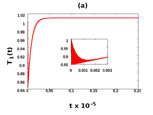
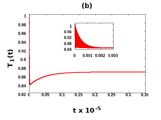
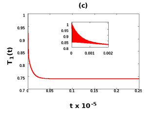
Figure 1: Time dynamics of the cold qubit temperature for the configuration $\big{\{}B_{1}^{M},B_{2}^{M},B_{3}^{M}\big{\}}$. Here we depict the dependence of $T_{1}(t)$ on $t$ in the three operating regimes: (a) $\mathbf{S_{1}}$: for $\alpha_{1}=10^{-3}$, $\alpha_{2}=10^{-4}$, $\alpha_{3}=10^{-2}$, (b) $\mathbf{S_{2}}$: for $\alpha_{1}=10^{-4}$, $\alpha_{2}=10^{-4}$, $\alpha_{3}=10^{-2}$ and (c) $\mathbf{S_{3}}$: for $\alpha_{1}=10^{-4}$, $\alpha_{2}=10^{-3}$ and $\alpha_{3}=10^{-2}$. The transient behaviour near $t\times 10^{-5}\approx 0$ is shown in the insets of the main figures in panels (a), (b) and (c). The system parameters are chosen to be $E_{1}=E_{3}=1.0$ and $g=0.8$. The temperature of the thermal baths are taken as $\tau_{1}=\tau_{2}=1.0$ and $\tau_{3}=2.0$ and the cut off frequency of all the baths is taken to be $\Omega=10^{3}$. All the quantities plotted are dimensionless.

It is already known that there are three operating regimes of an ideal quantum absorption refrigerator with the configuration $\big{\{}B_{1}^{M},B_{2}^{M},B_{3}^{M}\big{\}}$, depending on the qubit-bath interaction strengths, $\alpha_{i}$ for $i=1,2,3$, of the three-qubit three-bath model Sreetama . An example of these three scenarios is described below in a regime, where the coupling between the qubits are taken to be strong, i.e., $g\approx E_{i}$.

$\mathbf{S_{1}}$: TC without SSC. Fig. 1-(a) shows a refrigeration of the cold qubit in the regime where transient cooling occurs without the occurance of steady state cooling. The minimum of the transient temperature is acquired for $\overline{T}_{1}^{C}\approx 0.84$. After a finite time, the temperature of the cold bath saturates at a value higher than the initial temperature $\tau_{1}=1$, displaying a characteristic of steady state heating.

$\mathbf{S_{2}}$: TC better than SSC. From Fig. 1-(b) we can realise a situation where both the transient and steady state cooling occur, but the transient cooling is better than the steady state one. Comparing with Fig. 1-(a), it is noted that in the transient region, the behaviour of the system remains qualitatively same attaining a minimum temperature at $T_{1}^{\prime C}\approx 0.84$. Also, there is an additional feature of steady state cooling ($T_{1}^{\prime S}\approx 0.88$) which is completely non-existent in the previous case ($\mathbf{S_{1}}$).

$\mathbf{S_{3}}$: SSC better than TC. Fig 1-(c) describes a operative region of the refrigerator where both the transient and steady state cooling occur, but the steady state cooling is better than the transient one.

In all the three situations $\mathbf{S_{1}}$, $\mathbf{S_{2}}$ and $\mathbf{S_{3}}$, we get a specific parameter region of $\big{\{}\alpha_{1},\alpha_{2},\alpha_{3}\big{\}}$ for the operation of the refrigerators. For the convenience of notation we will denote the specific regions as $\big{\{}\alpha_{1}^{S_{i}},\alpha_{2}^{S_{i}},\alpha_{3}^{S_{i}}\big{\}}$ for the corresponding situation $\mathbf{S_{i}}$ with $i=1,2$ and $3$.

III Effect of non-Markovianity on the refrigeration

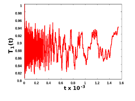
Figure 2: Time dynamics of the cold qubit temperature for the configuration $\big{\{}B_{1}^{NM},B_{2}^{NM},B_{3}^{NM}\big{\}}$. Here we demonstrate $T_{1}(t)$ vs. $t$ when all the three baths are taken to be non-Markovian. The system parameters and the temperature of the baths are taken to be the same as in Fig. 1. The bath frequencies are taken as $\nu_{1}=\nu_{2}=\nu_{3}=1.0$, and the dimension of each of the bath is taken $N=2$. All the quantities plotted along the horizontal and the vertical axes are dimensionless.

A Markovian situation is a very special case having some strict restrictions on the thermal baths, whereas the existence of a non-Markovian bath in the nature is more likely. So, there may occur some erroneous tuning of the parameters of the thermal baths, and any of the three bath or all the three baths may show non-Markovianity. Hence, the effect of non-Markovian baths on the refrigeration is needed to be studied. Let us first discuss the case, where all the three baths in the three-qubit three-bath refrigerator setup are non-Markovian i.e., the configuration is $\big{\{}B_{1}^{NM},B_{2}^{NM},B_{3}^{NM}\big{\}}$. The $NM$ in the superscripts stands for the non-Markovian baths. In this case, the system bath interaction is considered to form a “spin-star” configuration. There are $N+1$ number of spins, among which $N$ are lying on the surface of a sphere with one single central spin at equal distance from the spins on the surface. The central spin comprises the open system and is supposed to belong to a two dimensional Hilbert space $\mathcal{H}_{A}$, while the surrounding spins constitute the environment associated with a Hilbert space $\mathcal{H}_{B}$ whose dimension is an $N$-fold tensor product of two dimensional spaces. The local Hamiltonian of the $i^{\text{th}}$ bath is taken as

$$H_{B_{i}^{NM}}=\hbar\nu_{i}J_{i}^{+}J_{i}^{-},$$ (9)

where

$$J_{i}^{\pm}=\sum_{i}^{N}\sigma_{(i)}^{\pm}\quad\text{and}\quad\sigma_{i}^{\pm}=\frac{\sigma_{x}^{i}\pm i\sigma_{y}^{i}}{2},$$ (10)

with $\nu_{i}$ being the frequency of $B_{i}^{NM}$. The interaction between the central spin and neighbouring spins is taken to be of the form of the Heisenberg $XY$ interaction Breuer1 , given by

$$H_{SB_{i}^{NM}}=2K\alpha_{0}\Big{(}\sigma_{i}^{+}J_{i}^{-}+\sigma_{i}^{-}J_{i}^{+}\Big{)}.$$ (11)

Here, $\alpha_{0}$ stands for the dimensionless interaction strength. For our entire analysis, we have chosen $\alpha_{0}=0.5$. The time dynamics of the reduced three-qubit system after tracing out the baths is controlled by the following equation,

$$\rho_{s}(t)=\text{Tr}_{B}\big{[}e^{-i(H_{S}+H_{I})}\rho(t)e^{i(H_{S}+H_{I})}\big{]},$$ (12)

where $\rho(t)$ is the combined state of system-bath setup at time $t$.

The effect of cooling of the first qubit, for the configuration $\big{\{}B_{1}^{NM},B_{2}^{NM},B_{3}^{NM}\big{\}}$ is depicted in Fig. 2. The temperature $T_{1}(t)$ oscillates between $0.8$ and $0.96$. So, the minimum transient temperature attained by qubit-$1$ is less than the minimum transient $(\approx 0.84)$ and steady state temperatures $(>0.86)$ for the settings in Figs.1-(a) and (b), but is not better than the situation depicted in Fig.1-(c), attained for the ideal Markovian cases. Therefore, the transient cooling of the first qubit can be enhanced for certain choices of the bath parameters, once all the three baths attached to the system are made non-Markovian. An important point is to be noted that, although the rapidity of oscillation of $T_{1}(t)$ reduces with the increase of time, but the steady state is not reached due to the non-Markovian nature of the system-bath interaction, or it may appear at a larger timescale. So, a steady state cooling may not be attainable for the situation where all the three baths are non-Markovian.

Since some baths (with some restrictions) can be considered as a member of a Markovian family and some non-Markovian baths have their Markovian limits, so it is justifiable to have a situation where among the three baths one or two will be Markovian and the remaining are not so. The time evolution of the three-qubit system as a whole in presence of such a mixture of local Markovian and non-Markovian environments is given by the following equation Ghoshal

$$\frac{\partial\tilde{\rho}_{s}(t)}{\partial t}=\mathcal{L}(\tilde{\rho}_{s}(t))=-\frac{i}{K}[H_{S},\tilde{\rho}_{s}(t)]$$

$$+\frac{\hbar}{K}\sum_{\{i_{m}\}}\mathcal{D}_{M_{i_{m}}}(\tilde{\rho}_{s}(t))+\frac{\hbar}{K}\sum_{\{i_{n}\}}\mathcal{D}_{NM_{i_{n}}}(\rho_{sB_{\{i_{n}\}}^{NM}}(t)).\;\;\;\;$$ (13)

Here, each of $i_{m}$ and $i_{n}$ stands for the $i^{\text{th}}$ qubit, connected to $i^{\text{th}}$ bath which can be either $m^{\text{th}}$ Markovian or $n^{\text{th}}$ non-Markovian, with $m$ and $n$ are the total number of Markovian and non-Markovian baths respectively. The reduced state of the system $\tilde{\rho}_{s}(t)$ is given by $\tilde{\rho}_{s}(t)=\text{Tr}_{B_{\{i_{n}\}}}\big{(}\rho_{sB_{\{i_{n}\}}^{NM}}(t)\big{)}$, where $\rho_{sB_{\{i_{n}\}}^{NM}}(t)$ is the system state correlated with all the non-Markovian baths. $\mathcal{D}_{M_{i_{m}}}(\tilde{\rho}_{s}(t))$ is the dissipative term coming from the interaction between $i^{\text{th}}$ qubit and $i^{\text{th}}$ bath, which is a Markovian bosonic one, having the form same as Eq. (8). The Lindblad operators of this dissipative term corresponding to $i_{m}=i$ can be presented as $L_{i}^{\omega^{\prime}}$ for $i=1$, $2$ and $3$ and has the same structure as in Eq. (B). $\mathcal{D}_{NM_{i_{n}}}(\rho_{sB_{\{i_{n}\}}^{NM}}(t))$ is the same coming from the $i^{\text{th}}$ qubit-bath interaction, for which the bath is non-Markovian, given by

$$\mathcal{D}_{NM_{i_{n}}}(\rho_{sB_{\{i_{n}\}}^{NM}}(t))=-\frac{i}{\hbar}\text{Tr}_{B_{i_{n}}^{NM}}\Big{[}H_{SB_{i_{n}}^{NM}},\rho_{sB_{\{i_{n}\}}^{NM}}(t)\Big{]}.$$ (14)

The choice of spin star model as a non-Markovian bath ensures that the reduced subsystem of the first qubit is diagonal in the eigenbasis of the system Hamiltonian, hence curtailing any ambiguity regarding the definition of local temperature for the combination of local Markovian and non-Markovian evolution. We now replace the Markovian baths of the ideal absorption refrigerator by non-Markovian reservoirs successively and investigate the effect of a mixed set of local environments on the transient as well as the steady state cooling of the first qubit. We refer to the usual three-qubit three Markovian baths setup to be an “ideal” one and after replacing any of the Markovian bath with a non-Markovian one, we denote the situations as “altered” scenarios. In all the three altered setups, $\mathbf{S_{1}}$, $\mathbf{S_{2}}$ and $\mathbf{S_{3}}$, the parameters of the Markovian baths, $\alpha_{i}$ for $i=1,2$ and $3$, are same as in ideal $\mathbf{S_{1}}$, $\mathbf{S_{2}}$ and $\mathbf{S_{3}}$ scenarios respectively, and all the parameters of the non-Markovian baths are same as in Fig. 2. In this paper, we have considered four altered scenarios by taking two situations with $m=2$ and $n=1$ in Eq. (III) with the bath configurations: $\mathcal{A}_{1}^{S_{i}}\equiv\big{\{}B_{1}^{NM},B_{2}^{M},B_{3}^{M}\big{\}}$ and $\mathcal{A}_{2}^{S_{i}}\equiv\big{\{}B_{1}^{M},B_{2}^{M},B_{3}^{NM}\big{\}}$, and two situations with $m=1$ and $n=2$ with the bath configurations: $\mathcal{A}_{3}^{S_{i}}\equiv\big{\{}B_{1}^{NM},B_{2}^{M},B_{3}^{NM}\big{\}}$ and $\mathcal{A}_{4}^{S_{i}}\equiv\big{\{}B_{1}^{M},B_{2}^{NM},B_{3}^{NM}\big{\}}$. The superscripts, $S_{i}$, denote the corresponding ideal situations $\mathbf{S_{1}}$, $\mathbf{S_{2}}$ and $\mathbf{S_{3}}$ respectively for $i=1,2$ and $3$. Therefore the parameter spaces corresponding to these four scenarios $\mathcal{A}_{1}^{S_{i}}$, $\mathcal{A}_{2}^{S_{i}}$, $\mathcal{A}_{3}^{S_{i}}$ and $\mathcal{A}_{4}^{S_{i}}$ are respectively $\big{\{}\alpha_{0},\alpha_{2}^{S_{i}},\alpha_{3}^{S_{i}}\big{\}}$, $\big{\{}\alpha_{1}^{S_{i}},\alpha_{2}^{S_{i}},\alpha_{0}\big{\}}$, $\big{\{}\alpha_{0},\alpha_{2}^{S_{i}},\alpha_{0}\big{\}}$ and $\big{\{}\alpha_{1}^{S_{i}},\alpha_{0},\alpha_{0}\big{\}}$. The situations $\mathcal{A}_{1}^{S_{1}}$, $\mathcal{A}_{3}^{S_{1}}$ and $\mathcal{A}_{4}^{S_{2}}$ are same as $\mathcal{A}_{1}^{S_{2}}$, $\mathcal{A}_{3}^{S_{2}}$ and $\mathcal{A}_{4}^{S_{3}}$ respectively, since $\alpha_{1}^{S_{2}}=\alpha_{1}^{S_{3}}$, $\alpha_{2}^{S_{3}}=\alpha_{2}^{S_{2}}$ and $\alpha_{3}^{S_{1}}=\alpha_{3}^{S_{2}}$. Further, we compare the three-qubit refrigerator model with one and two-qubit self-sustaining thermal devices kept in contact with spin-baths, which also exhibit refrigeration in certain situations.

III.1 Cooling of the cold qubit in the altered situation of $\mathcal{A}_{1}^{S_{i}}$

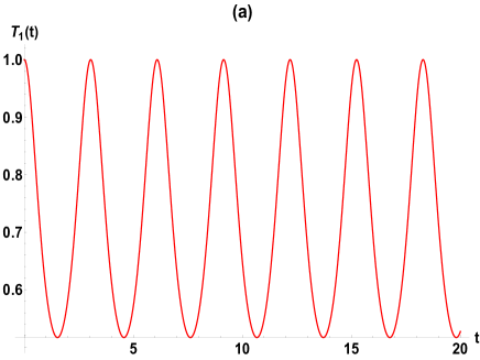
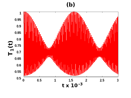
Figure 3: Panel (a) depicts the single-qubit scenario which is kept in contact with a spin-environment. The temperature of the qubit, $T_{1}(t)$, is plotted as a function of time, $t$. Panel (b): Effect of mixed environments on a two-qubit thermal device, which is self-sustaining under the condition $E_{1}^{2}=-E_{2}^{2}$. The configuration is $\mathcal{Q}_{2}=\big{\{}B_{1}^{SB},B_{3}^{BM}\big{\}}$, where $N=1$. Here $E_{1}^{2}=0.5$, the temperature of the first bath is $T_{1}^{2}=1$, and second bath is $T_{2}^{2}=2$. All quantities plotted are dimensionless.

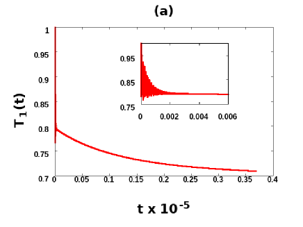
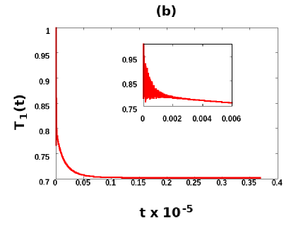
Figure 4: Effects of mixed set of local environments on cooling for altered setups of $\big{\{}\alpha_{0},\alpha_{2}^{S_{i}},\alpha_{3}^{S_{i}}\big{\}}$. Here we take the parameter space of $\mathbf{S_{1}}$, $\big{\{}\alpha_{1}^{S_{1}},\alpha_{2}^{S_{1}},\alpha_{3}^{S_{1}}\big{\}}$ and $\mathbf{S_{3}}$, $\big{\{}\alpha_{1}^{S_{3}},\alpha_{2}^{S_{3}},\alpha_{3}^{S_{3}}\big{\}}$, for ideal Markovian situation and plot the dependence of $T_{1}(t)$ vs. $t$ by replacing the first Markovian bath with a non-Markovian one. The situation of $\mathcal{A}_{1}^{S_{i}}$ with the configuration $\big{\{}\alpha_{0},\alpha_{2}^{S_{i}},\alpha_{3}^{S_{i}}\big{\}}$ is depicted in the two panels: (a) $\mathcal{A}_{1}^{S_{1}}$ with $\big{\{}\alpha_{0},\alpha_{2}^{S_{1}},\alpha_{3}^{S_{1}}\big{\}}$, (b) $\mathcal{A}_{1}^{S_{3}}$ with $\big{\{}\alpha_{0},\alpha_{2}^{S_{3}},\alpha_{3}^{S_{3}}\big{\}}$. The configuration of $\mathcal{A}_{1}^{S_{1}}$ matches with the $\mathcal{A}_{1}^{S_{2}}$ one for the chosen values of $\alpha_{2}$ and $\alpha_{3}$. The inset in panels (a) and (b) present a magnified version of the transient behaviour near the initial time of the main figure. The system parameters and the specifications for each of the Markovian and non-Markovian baths are taken same as in Figs. 1 and 2 respectively. All the quantities plotted along both the axes are dimensionless.

Let us first consider a situation where there is a single qubit attached to a spin-environment where the qubit-bath interaction is given by Eq. (11). The system Hamiltonian is considered to be $H^{1}=E_{1}^{1}\sigma_{z}/2$. The initial state is taken as a product of the thermal states of the qubit and bath, each of which are at temperature $T_{1}^{1}=1$. After the evolution, the final state is also diagonal, and we can calculate the temperature corresponding to the final state. If we consider the environment to consist of only a single spin, i.e. $N=1$ in Eq. (9), then the expression of the final temperature of the qubit, hence obtained, is given in Appendix A. It is noted that if $E_{1}^{1}<1$, then the temperature, $T_{1}(t)$, oscillates uniformly between $T_{1}(t)=1$ and some $T_{1}(t)<1$, but the envelope of temperature oscillations is linear and never converges to equilibrium. So there is an instance of transient refrigeration at certain times, although the maximum of the envelope never goes below unity(Fig. 3-(a)).

Next let us consider a two-qubit thermal device comprising of the cold qubit and one of the other two qubits of the three-qubit absorption refrigerator. So the configuration is either $\mathcal{Q}_{1}=\big{\{}B_{1}^{NM},B_{2}^{M}\big{\}}$ or $\mathcal{Q}_{2}=\big{\{}B_{1}^{NM},B_{3}^{M}\big{\}}$. The interactions between the two qubits for the configurations $\mathcal{Q}_{1}$ and $\mathcal{Q}_{2}$ are $H_{1}=|01\rangle\langle 10|+|10\rangle\langle 01|$ and $H_{2}=|00\rangle\langle 11|+|11\rangle\langle 00|$ respectively. Let us first look at the case $\mathcal{Q}_{1}$. The local Hamiltonian is $H^{2}=(E_{1}^{2}/2)\sigma_{z}^{(1)}+(E_{2}^{2}/2)\sigma_{z}^{(2)}$. The two eigenstates of $H^{2}$, $\ket{01}$ and $\ket{10}$, are degenerate if $E_{1}^{2}=E_{2}^{2}$, and therefore the swapping, $\ket{10}\leftrightarrow\ket{01}$, can be done without any input of external energy. However under this condition, the initial temperature of the first qubit being $T_{1}$ and the second qubit being $T_{2}$, satisfying $\tau_{1}=T_{1}\leq T_{2}$, one always obtains the final temperature $T_{1}(t)>\tau_{1}$, and there is no refrigeration. On the other hand, for the configuration, $\mathcal{Q}_{2}$, the self-sustained condition is given by $E_{1}^{2}=-E_{2}^{2}$, where no external energy input is needed. Under this condition, keeping $T_{1}\leq T_{2}$, and $E^{2}_{1}<1$, there is an instance of refrigeration, and we depict the particular case of $E^{2}_{1}=0.5$ in Fig.3-(b). So refrigeration is observed under certain conditions in the single and two-qubit scenarios, when the first qubit is attached to spin-bath, but in none of these situations steady state cooling is achieved.

Let us now move to the three-qubit case. We consider a three-qubit ideal quantum absorption refrigerator operating in the parameter regime $\mathbf{S_{1}}$. We now replace the Markovian bath attached to the cold qubit by a non-Markovian one, which gives the configuration $\mathcal{A}_{1}^{S_{1}}$, i.e., $\big{\{}B_{1}^{NM},B_{2}^{M},B_{3}^{M}\big{\}}$. The system-bath interaction is now governed by $\tilde{H}_{1}=H_{SB_{1}^{NM}}+\sum_{i=2}^{3}H_{SB_{i}^{M}}$. In Fig. 4-(a) we depict the dynamics of the temperature of the first qubit in this scenario. We observe that the refrigeration of the refrigerator is present here. The transient temperature $T_{1}(t)$ approaches a minimum $>0.75$, which is less than the same of the corresponding ideal Markovian baths case $\overline{T}_{1}^{C}$, and in course of time slowly attains a steady state temperature with temperature $\approx 0.7$. So, in this altered situation we acquire both transient cooling (TC) and steady state cooling (SSC), while for the ideal Markovian case, the SSC was non-existent in $\mathbf{S_{1}}$ (see Fig 1-(a)). If we consider the parameter regime, $\mathbf{S_{2}}$, and substitute the first Markovian bath by a non-Markovian one, we get the configuration $\mathcal{A}_{1}^{S_{2}}$. This configuration is qualitatively the same as in $\mathcal{A}_{1}^{S_{1}}$, since $\alpha_{2}$ and $\alpha_{3}$ are equal in both these cases.

We now look at the effect of combined local Markovian and non-Markovian evolution on the operation of an ideal absorption refrigerator with the bath combination $\big{\{}B_{1}^{NM},B_{2}^{M},B_{3}^{M}\big{\}}$, but in the parameter space $\mathbf{S_{3}}$. In this case, the minimum of the transient temperature $T^{C}_{1_{min}}<T_{1}^{\prime C}$ of the ideal case, and it approaches the steady state with temperature $T_{1}^{S}<{T^{\prime}}_{1}^{S}$. So, here also, the refrigeration of the refrigerator is prevalent, and both TC and SSC is observed. In the case of $\mathcal{A}_{1}^{S_{3}}$, we can attain a steady state cooling with a temperature of the first qubit $\approx 0.7$, while in the ideal case of $S_{3}$, the steady state temperature is $\approx 0.75$. Hence, compared to Fig. 1-(c), an enhancement occurs both in the transient cooling and the steady state cooling when compared with the ideal scenario $\mathbf{S_{3}}$. Therefore, we can infer that, a reduction of the temperature of cold qubit is clearly visible in the transient and steady state regime for this altered setup, $\mathcal{A}_{1}^{S_{i}}$.

Therefore, the replacement of the Markovian bath attached to the cold qubit of an ideal absorption refrigerator in the operating regime $\mathbf{S_{1}}$ (or $\mathbf{S_{2}}$), enhance the transient cooling by reducing the temperature of the cold qubit below the cooling obtained in the ideal Markovian case $(<\overline{T}_{1}^{C})$. Moreover, the system equilibriates towards a steady state temperature in this altered situation of $\mathbf{S_{1}}$ (or $\mathbf{S_{2}}$). Similarly, substituting the first Markovian reservoir by a non-Markovian one for the setting $\mathbf{S_{3}}$, one attains an improved refrigeration both in the transient state and steady state regimes. So, the results in this subsection depict that if we substitute the Markovian bath attached to the cold qubit by a spin-environment, both transient and steady state cooling can be achieved, which is better than the ideal Markovian case. Further, we compare the situation $\mathcal{A}_{1}^{S_{i}}$ with the single-qubit case. For the single-qubit, we find that refrigeration is non-existent unless $E_{1}^{1}<1$, while in the three-qubit scenario, we always consider $E_{1}=E_{3}=1$. Also, unlike the case of $\mathcal{A}_{1}^{S_{i}}$, the final temperature in the single-qubit situation does not attain a staedy state, although it periodically goes below its initial temperature, $T_{1}^{1}=1$ (compare Figs. 3-(a) and  4). Now if we ompare $\mathcal{A}_{1}^{S_{i}}$ with the setting $\mathcal{Q}_{2}$, we see that refrigeration is present in both the settings, but again in the two-qubit case, $E_{1}^{2}$ has to be less than unity. Also, unlike $\mathcal{A}_{1}^{S_{i}}$, the oscillations in $\mathcal{Q}_{2}$ are persistent and steady state is not attained (compare Figs. 3-(b) and  4). Thus attainment of steady state cooling is a distinct feature of the quantum absorption refrigerator consisting of three qubits and not less than that.

III.2 Cooling of the cold qubit in the altered situation of $\mathcal{A}_{2}^{S_{i}}$

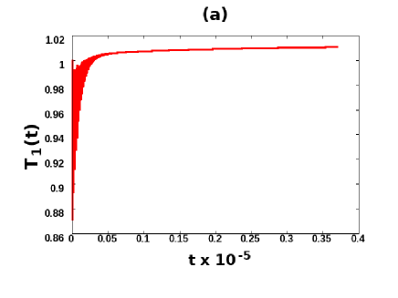
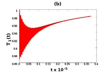
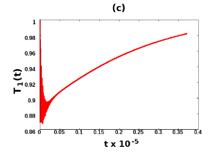
Figure 5: Effects of mixed set of local environments on cooling for altered setups of $\big{\{}\alpha_{0}^{S_{i}},\alpha_{2}^{S_{i}},\alpha_{3}\big{\}}$. Here we take the parameter space of $\mathbf{S_{1}}$, $\big{\{}\alpha_{1}^{S_{1}},\alpha_{2}^{S_{1}},\alpha_{3}^{S_{1}}\big{\}}$ , $\mathbf{S_{2}}$, $\big{\{}\alpha_{1}^{S_{2}},\alpha_{2}^{S_{2}},\alpha_{3}^{S_{2}}\big{\}}$ and $\mathbf{S_{3}}$, $\big{\{}\alpha_{1}^{S_{3}},\alpha_{2}^{S_{3}},\alpha_{3}^{S_{3}}\big{\}}$, for ideal Markovian situation and plot the dependence of $T_{1}(t)$ vs. $t$ by replacing the third Markovian bath with a non-Markovian one. The situation of $\mathcal{A}_{2}^{S_{i}}$ with the configuration $\big{\{}\alpha_{0}^{S_{i}},\alpha_{2}^{S_{i}},\alpha_{3}\big{\}}$ is depicted in the three panels: (a) $\mathcal{A}_{2}^{S_{1}}$ with $\big{\{}\alpha_{0}^{S_{1}},\alpha_{2}^{S_{1}},\alpha_{3}\big{\}}$, (b) $\mathcal{A}_{2}^{S_{2}}$ with $\big{\{}\alpha_{0}^{S_{2}},\alpha_{2}^{S_{2}},\alpha_{3}\big{\}}$ and (c) $\mathcal{A}_{2}^{S_{3}}$ with $\big{\{}\alpha_{0}^{S_{3}},\alpha_{2}^{S_{3}},\alpha_{3}\big{\}}$. The system parameters and the specifications for each of the Markovian and non-Markovian baths are taken same as in Figs. 1 and 2 respectively. All the quantities plotted along both the axes are dimensionless.

We begin this subsection by considering the ideal three-qubit scenario where all the three baths are Markovian, and substitute the bath, which is not connected to the cold qubit, by a non-Markovian one. We consider the three parameter regimes of $\mathbf{S_{1}}$, $\mathbf{S_{2}}$ and $\mathbf{S_{3}}$, and look at the effect of replacing the bosonic bath attached to the third qubit of the “ideal” scenario into a non-Markovian one, i.e. $\big{\{}B_{1}^{M},B_{2}^{M},B_{3}^{NM}\big{\}}$. The situation is qualitatively same for $\big{\{}B_{1}^{M},B_{2}^{NM},B_{3}^{M}\big{\}}$ configuration also (not shown). If we substitute any one of the second or third bosonic baths with a non-Markovian one, say the third one, i.e., the configuration $\mathcal{A}_{2}^{S_{1}}$ $\big{(}\big{\{}B_{1}^{M},B_{2}^{M},B_{3}^{NM}\big{\}}\big{)}$, we obtain only TC but do not obtain SSC as evident from Fig. 5-(a). In this situation, the minimum transient temperature is $<0.88$, which at steady state regime converges to a value $>1$. Similarly for the configuration $\mathbf{S_{2}}$, if the third qubit is connected to the non-Markovian spin-bath while the others being Markovian, i.e., $\mathcal{A}_{2}^{S_{2}}$, transient cooling is evident but steady state cooling may not be obtained, and the refrigeration of the refrigerator is present in the transient region only. See Fig. 5-(b). Here the minimum transient temperature, $<0.88$, and the steady state temperature, $\approx 0.98$, are greater than the corresponding minimum transient temperature and the equilibrium temperature of the final state in the corresponding ideal Markovian case. This feature is different from the $\mathcal{A}_{1}^{S_{i}}$ scenario, where there was an advantage over the corresponding ideal Markovian scenarios. Similarly, the configuration $\mathcal{A}_{2}^{S_{3}}$ exhibits transient cooling of the first qubit as depicted in Fig.(5-(c)). The minimum transient temperature lies beneath $\approx 0.88$ and equilibriates to a value $\approx 0.98$. So in the setting, $\mathcal{A}_{2}^{S_{i}}$, the action of the refrigerator in the transient regime still persists but without any advantage over the “ideal” Markovian case, and also showing instances of steady state heating. Hence, only TC is obtained but with no advanatge over the “ideal” Markovian scenario with the Markovian and non-Markovian bath ratio 2:1, if the first qubit is not kept in contact with the non-Markovian environment. Moreover, though the oscillations vary within a certain range of temperature in the transient region, the temperatures for all these three cases tend to attain an equilibrium at some large timescales. So attainability of steady state is also a feature noted in this situation.

III.3 Cooling of the cold qubit in the altered situation of $\mathcal{A}_{3}^{S_{i}}$

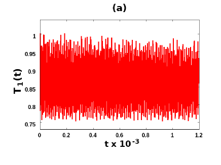
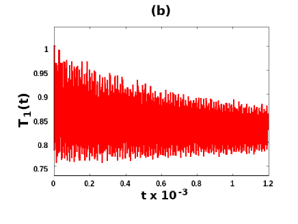
Figure 6: Effects of mixed set of local environments on cooling for altered setups of $\big{\{}\alpha_{0},\alpha_{2}^{S_{i}},\alpha_{3}\big{\}}$. Here we take the parameter space of $\mathbf{S_{1}}$, $\big{\{}\alpha_{1}^{S_{1}},\alpha_{2}^{S_{1}},\alpha_{3}^{S_{1}}\big{\}}$ , $\mathbf{S_{2}}$, $\big{\{}\alpha_{1}^{S_{2}},\alpha_{2}^{S_{2}},\alpha_{3}^{S_{2}}\big{\}}$ and $\mathbf{S_{3}}$, $\big{\{}\alpha_{1}^{S_{3}},\alpha_{2}^{S_{3}},\alpha_{3}^{S_{3}}\big{\}}$, for ideal Markovian situation and plot the dependence of $T_{1}(t)$ vs. $t$ by replacing the first and third Markovian baths with non-Markovian ones. The situation of $\mathcal{A}_{2}^{S_{i}}$ with the configuration $\big{\{}\alpha_{0},\alpha_{2}^{S_{i}},\alpha_{3}\big{\}}$ is depicted in the two panels: (a) $\mathcal{A}_{2}^{S_{1}}$ with $\big{\{}\alpha_{0},\alpha_{2}^{S_{1}},\alpha_{3}\big{\}}$ and (b) $\mathcal{A}_{2}^{S_{3}}$ with $\big{\{}\alpha_{0},\alpha_{2}^{S_{3}},\alpha_{3}\big{\}}$. The configuration of $\mathcal{A}_{3}^{S_{1}}$ matches with the $\mathcal{A}_{3}^{S_{2}}$ one for the chosen values of $\alpha_{2}$. The system parameters and the specifications for each of the Markovian and non-Markovian baths are taken same as in Figs. 1 and 2 respectively. All the quantities plotted along both the axes are dimensionless.

Here we consider an ideal three-qubit quantum refrigerator where all the three qubits are initially attached to Markovian baths, and two of them, say first and third one, are replaced by a spin-environment. So, here we consider the setting $\mathcal{A}_{3}^{S_{i}}$, i.e., $\big{\{}B_{1}^{NM},B_{2}^{M},B_{3}^{NM}\big{\}}$, where the system-bath interaction is governed by $\tilde{H}_{1}=\sum_{i=2}^{3}H_{SB_{1}^{NM}}+H_{SB_{i}^{M}}$. The features obtained in this setting are qualitatively same for the configuration, $\big{\{}B_{1}^{NM},B_{2}^{NM},B_{3}^{M}\big{\}}$ (not shown). Let us first look at the configuration $\mathcal{A}_{3}^{S_{1}}$, as depicted in 6-(a). The transient temperature $T_{1}(t)$ oscillates rapidly between $0.75$ and $1.0$ with its magnitude never surpassing unity. The minima of $T_{1}(t)$ varies around $\approx 0.75$, which shows refrigeration along with an enhancement in cooling of the first qubit than the minimum transient temperature of the corresponding ideal Markovian case. Compare Figs. 1-(a) and 6-(a). The setting $\mathcal{A}_{3}^{S_{2}}$ is qualitatively same as the previous case, $\mathcal{A}_{3}^{S_{1}}$ because of the choice of $\alpha_{2}$. Moreover,the attainment of equilibrium is non-existent in this scenario in a sufficiently large time-scale.

Next we consider the parameters corresponding to the configuration, $\mathcal{A}_{3}^{S_{3}}$, where we observe similar features. The transient temperature, $T_{1}(t)$, varies between $\approx 0.75$ and $1.0$, and the envelope of oscillations narrows down within the observed time. It may or may not reach equilibrium at large times. The refrigeration, however, is existent and the minimum transient temperature in this case($\approx 0.75$) is less than the minimum transient temperature in the corresponding ideal Markovian case 1-(c), although not less than its steady state temperature. Therefore, substituting any two Markovian baths including the first one is beneficial as this enhance the transient cooling, but the increase of non-Markovianity restrict the attainability of the steady state cooling. One distinct nature of this $m=1$, $n=2$ cases is that, the oscillations in $T_{1}(t)$ consistently persist with undiminished amplitudes and do not tend to saturate in a sufficiently large time-scale. This behaviour appears with the increase in the number of non-Markovian baths and qualitatively resembles the situation where all the three baths are non-Markovian. Compare with Fig. 2.

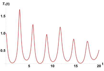
Figure 7: A two-qubit system in which both the qubits are kept in contact with spin-environments. The temperature of the qubit, $T_{1}(t)$, is plotted as a function of time, $t$. The two-qubit thermal device is self-sustaining under the condition $E_{1}^{2}=E_{2}^{2}$. The configuration is $\big{\{}B_{1}^{SB},B_{3}^{SB}\big{\}}$, where the spin-bath has $N=1$. Here $E_{1}^{2}=0.1$, the temperature of the first bath is $T_{1}^{2}=1$, and second bath is $T_{2}^{2}=2$. All quantities plotted are dimensionless.

Next we compare the results obtained using the configuration, $\mathcal{A}_{3}^{S_{i}}$, with the single-qubit case. In the single-qubit scenario, refrigeration effect is present with periodic oscillations under the condition $E_{1}^{1}<1$ and not with $E_{1}^{1}=1$. But in the three-qubit situation, we always consider $E_{1}=E_{3}=1$. Moreover, in the single-qubit case, the envelope of oscilllations does not vary with time, a feature similar to $\mathcal{A}_{3}^{S_{1}}$ (refer to figures 3-(a) and  6-(a)). While, for $\mathcal{A}_{3}^{S_{3}}$, similar transient cooling is existent but the envelope narrows down with time (refer to Fig. 6-(b)). The non-attainment of equilibrium is also another feature noted in both these cases.

We now compare the three-qubit quantum absorption refrigerator under the configuration, $\mathcal{A}_{3}^{S_{i}}$, with the relevant two-qubit cases. We saw previously that the configuration $\mathcal{Q}_{1}$ does not provide a self-sustained two-qubit refrigerator. So we compare the two-qubit configuration,$\mathcal{Q}_{2}$, with the three-qubit configuration, $\mathcal{A}_{3}^{S_{i}}$. Again, in the two-qubit case, refrigeration is possible only when $E_{1}^{2}<1$ while in the three-qubit setup, cooling occurs when $E_{1}=E_{3}=1$. Both the cases depict a refrigeration effect without attaining equilibrium, although the envelope of the two plots are different. Compare Figs. 6-(b) and  3-(b).

Next, we also consider a two-qubit situation where both the qubits are attached to spin-baths, i.e. the configuration is $\mathcal{Q}_{3}=\{B^{NM}_{1},B^{NM}_{2}\}$. The local Hamiltonian is $H^{2}=(E_{1}^{2}/2)\sigma_{z}^{(1)}+(E_{2}^{2}/2)\sigma_{z}^{(2)}$. The two qubits interact via the interaction $H_{1}=|01\rangle\langle 10|+|10\rangle\langle 01|$, under the self-sustained condition, $E_{1}^{2}=E_{2}^{2}$. We measure the final temperature of the first qubit, which exhibits only transient cooling at certain times, and the final temperature of the first qubit, $T_{1}(t)$, sometimes rises above its initial temperature. Fig. 7, for example, depicts the case where $E_{1}^{2}=0.1$ and the spin-environment corresponds to $N=1$. Moreover, unlike the three-qubit case, cooling is not obtained here for $E_{1}^{2}\geq 1$.

III.4 Cooling of the cold qubit in the altered situation of $\mathcal{A}_{4}^{S_{i}}$

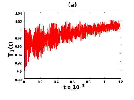
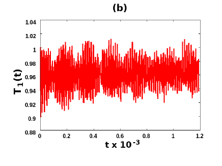
Figure 8: Effects of mixed set of local environments on cooling for altered setups of $\big{\{}\alpha_{0}^{S_{i}},\alpha_{2},\alpha_{3}\big{\}}$. Here we take the parameter space of $\mathbf{S_{1}}$, $\big{\{}\alpha_{1}^{S_{1}},\alpha_{2}^{S_{1}},\alpha_{3}^{S_{1}}\big{\}}$ , $\mathbf{S_{2}}$, $\big{\{}\alpha_{1}^{S_{2}},\alpha_{2}^{S_{2}},\alpha_{3}^{S_{2}}\big{\}}$ and $\mathbf{S_{3}}$, $\big{\{}\alpha_{1}^{S_{3}},\alpha_{2}^{S_{3}},\alpha_{3}^{S_{3}}\big{\}}$, for ideal Markovian situation and plot the dependence of $T_{1}(t)$ vs. $t$ by replacing the second and third bosonic baths with non-Markovian ones. The situation of $\mathcal{A}_{4}^{S_{i}}$ with the configuration $\big{\{}\alpha_{0}^{S_{i}},\alpha_{2}^{S_{i}},\alpha_{3}\big{\}}$ is depicted in the two panels: (a) $\mathcal{A}_{2}^{S_{1}}$ with $\big{\{}\alpha_{0}^{S_{1}},\alpha_{2},\alpha_{3}\big{\}}$ and (b) $\mathcal{A}_{2}^{S_{3}}$ with $\big{\{}\alpha_{0}^{S_{3}},\alpha_{2},\alpha_{3}\big{\}}$. The configuration of $\mathcal{A}_{4}^{S_{2}}$ matches with the $\mathcal{A}_{4}^{S_{3}}$ one for the chosen values of $\alpha_{1}$. The system parameters and the specifications for each of the Markovian and non-Markovian baths are taken same as in Figs. 1 and 2 respectively. All the quantities plotted along both the axes are dimensionless.

Let us now look into the case where the second and third qubits are connected to non-Markovian spin-baths while the first one is Markovian, i.e., the setting $\mathcal{A}_{4}^{S_{i}}$. Initially consider the ideal scenario when all the three baths are Markovian within the parameter region of $\mathbf{S_{1}}$. Now if we replace the baths attached with the second and third qubits to non-Markovian ones, it is observed that steady state cooling is not obtained, and the refrigeration of the refrigerator is almost destroyed. See Fig. 8-(a). In this case, the oscillations vary between temperatures $0.9$ and $1.02$, with the minimum transient temperature being $\approx 0.9$. The envelope of the oscillations gradually narrows down to a value greater that the initial temperature of the first qubit. Like in the previous subsection, here also the oscillations do not converge to a steady state within the observation period.

We now take the altered situation of $\mathbf{S_{2}}$, i.e. $\mathcal{A}_{4}^{S_{2}}$. For this setting (same with $\mathcal{A}_{4}^{S_{3}}$), we observe that the transient temperature of the cold qubit $T_{1}(t)$ begins to oscillate between $0.9$ and $<1.02$ without attaining a steady state. So here also, the envelope of temperature oscillations vary with time and no enhancement of the transient state cooling is achieved over the ideal Markovian situation compared to $\mathbf{S_{2}}$. Compare Figs. 8-(b) and 1-(b). An important feature to be noted here is that, like the situation of $\mathcal{A}_{3}^{S_{i}}$ with two of the baths made non-Markovian, here also for $\mathcal{A}_{4}^{S_{i}}$, the steady state is not attainable within the observation time. So, unattainability of steady state is a general feature of $m=1$ and $n=2$ configurations, and it does not solely depends on the parameter space of the Markovian bath, which is coupled to any of the qubits.

Therefore, we can conclude from the last two subsections that replacement of any two Markovian baths including the first one is beneficial as this enhance the transient cooling, but the increase of non-Markovianity restrict the attainability of the steady state cooling. On the other hand, replacing any of the second or third Markovian baths or both of them by a non-Markovian one by keeping the cold qubit attached with a Markovian bath, results in a deterioration of performance of the usual absorption refrigerator. So, one can attain a sufficient cooling of qubit-$1$ whenever it is connected to a non-Markovian environment, whatever be the nature of the baths attached to the other two.

Finally, the analysis in this section infers that, the effect of non-Markovian baths on the quantum absorption refrigerator, results an enhancement in cooling attainable in transient as well as the steady state regime in some cases (if attainable), when the cold qubit is attached to a non-Markovian bath. We can call the quantum refrigerators with the beneficial altered setups as “non-Markovian quantum refrigerators”. This reduction of temperature of the cold qubit with this non-Markovian setups owes its origin to the non-Markovianity incorporated to the bath attached to the first qubit. This leads to define a quantifier of non-Markovianity for a quantum absorption refrigerator discussed in the next section.

IV A measure of non-Markovianity

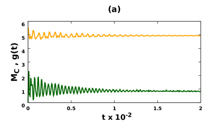
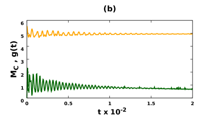
Figure 9: The measure of non-Markovianity against time t is plotted. The green curve depicts the proposed measure of non-Markovianity, $M_{C}$ scaled by a factor $\delta$, for the channel where only the first bath is non-Markovian and the orange curve represents the corresponding RHP measure, $g(t)$. Panel (a) depicts the non-Markovianity measures corresponding to the channel $M_{\overline{C_{1}}}$, and panel (b) refers to the same for channel $M_{\overline{C_{2}}}$. The quantities plotted along both axes are dimensionless.

We have already shown that the efficiency of a quantum absorption refrigerator can be enhanced if the cold qubit is attached with a non-Markovian spin-bath, instead of a Markovian bosonic one. While for ideal Markovian situations (among of the three cases of ideal $\mathbf{S_{1}}$, $\mathbf{S_{2}}$ and $\mathbf{S_{3}}$), the transient and steady state temperatures attain $\approx 0.84$ and $\approx 0.75$ respectively, and a replacement of the Markovian bath attached to the cold qubit with a non-Markovian one, can reduce the respective transient and steady state temperatures to $<0.8$ and $\approx 0.7$. Let us try to find the origin of the decrease of temperature. As we concentrate on the temperature of qubit-$1$, from now on we will focus on the time dynamics of the first qubit only.

Let us consider a two level system described by the Hamiltonian $H=KE^{\prime}_{0}|0\rangle\langle 0|+KE^{\prime}_{1}|1\rangle\langle 1|$ and the initial state of the system, $\rho^{\prime}(0)$, is taken to be diagonal in the eigenbasis of the Hamiltonian. Now suppose, a non-Markovian channel $N^{t}_{NM}$ is applied on the qubit for time $t$ which results an evolution of the system, such that the density matrix of the state remains diagonal in the eigenbasis of the Hamiltonian. The corresponding density matrix is given by $\rho^{\prime}_{NM}(t)=N^{t}_{NM}(\rho^{\prime}(0))=p(t)|0\rangle\langle 0|+(1-p(t))|1\rangle\langle 1|$. Similarly, if the qubit evolves through a Markovian channel $N^{t}_{M}$, one can obtain the dynamical state as $\rho^{\prime}_{M}(t)=N^{t}_{M}(\rho^{\prime}(0))=p^{\prime}(t)|0\rangle\langle 0|+(1-p^{\prime}(t))|1\rangle\langle 1|$. The dynamical temperatures corresponding to the non-Markovian $(T_{NM}^{t})$ and Markovian $(T_{M}^{t})$ processes are defined through the following relations

$$\bra{0}\rho^{\prime}_{NM}(t)\ket{0}=\frac{e^{-\frac{E^{\prime}_{0}}{T_{NM}^{t}}}}{e^{-\frac{E^{\prime}_{0}}{T_{NM}^{t}}}+e^{-\frac{E^{\prime}_{1}}{T_{NM}^{t}}}}=\alpha_{NM}$$

$$\bra{0}\rho^{\prime}_{M}(t)\ket{0}=\frac{e^{-\frac{E^{\prime}_{0}}{T_{M}^{t}}}}{e^{-\frac{E^{\prime}_{0}}{T_{M}^{t}}}+e^{-\frac{E^{\prime}_{1}}{T_{M}^{t}}}}=\alpha_{M}$$ (15)

respectively. Inverting these equations, one arrives at

$$T_{NM}^{t}-T_{M}^{t}=(E^{\prime}_{0}-E^{\prime}_{1})\Big{[}\frac{1}{\ln\big{(}\frac{1}{\alpha_{NM}}-1\big{)}}-\frac{1}{\ln\big{(}\frac{1}{\alpha_{M}}-1\big{)}}\Big{]}.$$ (16)

In this equation, the difference, $T_{NM}^{t}-T_{M}^{t}$, is a function of the parameters of the Markovian channel, $\alpha_{1},\alpha_{2}$ and $\alpha_{3}$. So the difference will vary with the choice of the channel parameters and may even give zero value corresponding to a particular choice of these three parameters. So we optimise over the channel parameters, $\alpha_{1},\alpha_{2}$ and $\alpha_{3}$, to give a generalized expression of the quantity in 16. Thus Eq. (16), with an optimisation over $\alpha_{M}$, can be visualized as a measure of non-Markovianity of an arbitrary quantum channel $C$ which manifests the deviation from its Markovian counterpart. We therefore define the quantity,

$$M_{C}=\Big{|}(E^{\prime}_{0}-E^{\prime}_{1})\Big{[}\frac{1}{\ln\big{(}\frac{1}{\alpha_{C}}-1\big{)}}-\text{min}_{\alpha_{M}}\frac{1}{\ln\big{(}\frac{1}{\alpha_{M}}-1\big{)}}\Big{]}\Big{|}$$ (17)

as a measure of non-Markovianity as this term quantifies the temperature difference of a system after passing through an arbitrary channel $C$, from the temperature obtained when passing through an optimal Markovian channel. This quantifier $M_{C}$ returns a positive value when the channel is non-Markovian, While for a Markovian channel, the quantifier is zero.

We now study the nature of the quantifier for the configuration of bath, $\mathcal{A}_{1}^{S_{i}}$, with the parameter regions $\mathcal{A}_{1}^{S_{1}}=\mathcal{A}_{1}^{S_{2}}$ and $\mathcal{A}_{1}^{S_{3}}$ as quantum channels, say $\overline{C_{1}}$, $\overline{C_{2}}$ respectively. The time dynamics of $M_{\overline{C_{1}}}$ and $M_{\overline{C_{2}}}$ are presented in Fig. 9-(a) and Fig. 9-(b) (the green curves) respectively. For clarity, the quantifier $M_{C}$ is scaled by a factor $\delta=20$ and plotted. Both $M_{\overline{C_{1}}}$ and $M_{\overline{C_{2}}}$ show similar features. The two curves depict a small but positive value of the quantifier $M_{C}$ when plotted against time. It is thus evident that the system exhibits a non-Markovian behaviour within the observed timescale in the altered scenario, $\mathcal{A}_{1}^{S_{i}}$.

It is a well established fact that the quantifiers of non-Markovianity are not all equivalent. So, here we consider a different measure of non-Markovianity, the Rivus-Huelga-Plenio (RHP) measure RHP , to comment on the equivalence between the measure, $M_{C}$, with a widely used quantifier of non-Markovianity. Suppose we can split a dynamical map from $0$ to $t+\epsilon$, with some intermediate time difference $\epsilon$, as

$$\mathcal{E}_{(t+\epsilon,0)}=\mathcal{E}_{(t+\epsilon,t)}\mathcal{E}_{(t,0)},$$ (18)

where $\mathcal{E}_{(t+\epsilon,t)}$ is a completely positive (CP) map, then the channel implemented by $\mathcal{E}_{(t+\epsilon,0)}$ is Markovian. The non-CP nature of $\mathcal{E}_{(t+\epsilon,t)}$ is given by

$$g_{\mathcal{E}}(t)=\lim_{\epsilon\rightarrow 0^{+}}\frac{f(t+\epsilon,t)-1}{\epsilon},$$ (19)

where $f(t+\epsilon,t)=||(\mathcal{E}_{(t+\epsilon,t)}\otimes\mathbf{I})(\ket{\phi}\bra{\phi})||_{1}$ with $\epsilon>0$. Here $\mathcal{E}_{(t+\epsilon,t)}$ represents an arbitrary channel between times $t$ and $t+\epsilon$, and $||A||_{1}$ is the trace norm defined by $\sqrt{A^{\dagger}A}$. The map, $\mathcal{E}_{(t+\epsilon,0)}$, is said to be Markovian if and only if $g_{\mathcal{E}}(t)=0$, otherwise $g_{\mathcal{E}}(t)>0$. Therefore, for a process to be non-Markovian, the quantity, $g_{\mathcal{E}}(t)>0$. Here $\ket{\phi}$ is a maximally entangled system-auxiliary state which is chosen to be $\frac{1}{\sqrt{2}}(\ket{00}_{SA}+\ket{11}_{SA})$ in this paper. The orange curves in Fig. 9-(a) and  9-(b) depict the behaviour of the RHP measure given in Eq. (19) for the non-Markovian channel $\overline{C}$. If the dynamics of a non-Markovian evolution be governed by $\frac{d\rho}{dt}=\mathcal{L}_{t}$, then in the limit $\epsilon\rightarrow 0$, Eq. (19) reduces to

$$g(t)=\lim_{\epsilon\rightarrow 0^{+}}\frac{||[\textbf{I}+(\mathcal{L}_{t}\otimes\textbf{I})\epsilon]|\phi\rangle\langle\phi|||_{1}-1}{\epsilon},$$ (20)

where $\mathcal{E}_{(t+\epsilon,t)}=e^{\mathcal{L}_{t}\epsilon}$. The orange curves in Fig. 9 has been plotted using this Eq. (20). The quantifier $g_{\overline{C}}(t)$ exhibits a positive value at a all times, which imply non-Markovianity in terms of the RHP measure at all timescales.

Figures 9-(a) and (b), depict the non-Markovianity of the respective channels $\overline{C}_{1}$ and $\overline{C}_{2}$, as quantified by the new measure, $M_{\overline{C}_{i}}$ for $i=1,2$ (green curve), and the RHP measure (orange curve). Comparing the green and orange curves in each of 9-(a) and (b), it is noted that in the observed times, both $M_{\overline{C}_{i}}$ and $g_{\overline{C}_{i}}$ are positive, which implies that non-Markovianity is key feature of the system which is depicted by both the measures. Our measure, therefore, captures the non-Markovianity present in the system which is also evident in terms of the RHP measure.

V Impact of Markovian noise on a non-Markovian quantum refrigerator

We have already observed the enhancement in the efficiency of cooling of a quantum absorption refrigerator in some cases, while using non-Markovian baths instead of the Markovian ones for the ideal setups. Those altered situations, advantageous over the relevant Markovian cases, are idealistic, and environmental noise or fluctuations can have non-negligible effects on the efficiency of refrigeration, as noise is ubiquitous in nature. So, if we want to implement such an altered refrigerator model in reality, it is useful to look at the scenario in presence of decoherence noise.

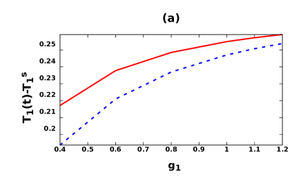
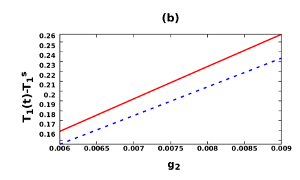
Figure 10: (a) Red solid curve gives the variation of the temperature difference in the steady state (at time $t=t_{s}$) between the first qubit and the steady state temperature ${T^{\prime}}_{1}^{S}$ against the noise strength $g_{1}$ when the refrigerator is placed in amplitude damping noise. Blue dashed curve represents the same difference but only at time $t_{s}/2$. The parameters chosen are $T_{N_{1}}=1.0$ and $\alpha=0.001$. The parameters plotted along both the axes are dimensionless. (b) When the refrigerator is placed under depolarizing noise, the red solid curve shows the fluctuation of the temperature difference in the steady state (at time $t=t_{s}$) between the first qubit and the steady state temperature ${T^{\prime}}_{1}^{S}$ against the noise strength $g_{2}$. The parameters considered are $T_{N_{2}}=1.0$ and $\alpha=0.01$. The difference at time $t_{s}/2$ is represented by the blue dashed curve. The quantities plotted along both the axes are dimensionless.

V.1 Noise model-I

A quantum absorption refrigerator is constructed by a three-qubit three-bath setup. In ideal situations, all the three baths are Markovian and in some altered cases, the bath attached to the cold qubit can be non-Markovian. Here we consider a three-qubit refrigerator in which the cold qubit is kept in a spin-environment (altered situation), along with being connected with a noisy Markovian environment, given by $\mathcal{N}_{1}(\cdot)$, where the argument is the altered refrigerator setup. In this paper, we have considered the noisy scenario $\mathcal{N}_{1}(\mathcal{A}_{1}^{S_{3}})$ , where the cold qubit is coupled to a non-Markovian spin-bath taken in the previous discussions and also to a Markovian bosonic environment $B^{M_{1}}$. The other two qubits are connected to bosonic baths as before. Therefore the configuration is $\big{\{}B_{1}^{NM,N_{1}},B_{2}^{M},B_{3}^{M}\big{\}}$, and the interaction Hamiltonian of the cold qubit and the Markovian environment $B^{M_{1}}$ is given by

$$H_{SB^{M_{1}}}=\sqrt{g_{1}}\int_{0}^{\Omega}\hbar\sqrt{\tilde{\omega}}d\omega h_{M_{1}}(\omega)(\sigma_{-}\eta_{\omega}^{M_{1}\dagger}+\sigma_{+}\eta_{\omega}^{M_{1}}).$$ (21)

Here $g_{1}$ is the dimensionless noise strength. All the other quantities are defined previously. The modified GKSL master equation for this noisy scenario is same as Eq. (III), with an extra dissipative term coming from the contribution of noisy Markovain environment. So, the GKSL master equation for this noisy scenario turns out to be

$$\frac{\partial\tilde{\rho}_{s}^{\mathcal{N}_{1}}(t)}{\partial t}=\frac{\partial\tilde{\rho}_{s}(t)}{\partial t}+\frac{\hbar}{K}g_{1}\mathcal{D}_{M_{1}}(\tilde{\rho}_{s}(t)).$$ (22)

Taking this noisy environment into consideration, the additional system operators are given by

$$\mathcal{A}^{E_{1}}_{1}=(|111\rangle\langle 011|+|100\rangle\langle 000|)\sqrt{2}$$

$$\mathcal{A}^{E_{1}+g}_{1}=\big{(}|110\rangle\langle+|+|-\rangle\langle 001|\big{)}$$

$$\mathcal{A}^{E_{1}-g}_{1}=\big{(}|+\rangle\langle 001|-|110\rangle\langle-|\big{)}.$$ (23)

The respective operators for the reverse processes is given by $\mathcal{A}^{-\omega}=\mathcal{A}^{\omega^{\dagger}}$. If an isolated qubit interacts with a reservoir via the interaction given in Eq. (21), then the time dynamics of the well-known amplitude damping channel is obtained for $T_{N_{1}}=0.0$, where $T_{N_{1}}$ is the temperature of the relevant bath.

In this case, we see that the system attains a steady state, and the temperature of the cold qubit at steady state is higher than the corresponding equilibrium temperature without the Markovian noise. If $g_{1}$ is made smaller $\approx 0.0001$, then the steady state temperature is almost equal to the one corresponding to Fig 4-(b), but is never less than that. So the Markovian noise deteriorates the operation of the refrigerator when compared with the non-Markovian case, though its behaviour as a refrigerator is still retained within a finite domain of $g_{1}$. It has been numerically examined that this noise model never gives advantage over the non-Markovian scenario if $g_{1}$ is non-zero, keeping the other parameters fixed in the previously mentioned values.

Fig.10-(a) depicts the scaling of the temperature difference between the cold qubit $(T_{1}(t))$ and the steady state temperature of Fig.(4-(b)) $(T_{1}^{s})$ vs the noise strength $g_{1}$. The solid red curve is at time $t=t_{s}=0.008$ when the system is at equilibrium and the blue dashed line represents the nature at $t=\frac{t_{s}}{2}$. There is a finite gap between the two curves for small $g_{1}$, and the difference gradually reduces prior to when the system stops behaving as a refrigerator.

V.2 Noise model II

In this subsection, we repeat the same formalism followed in the previous subsection but in presence of a different Markovian noise. Here we consider the configuration $\mathcal{N}_{2}(\mathcal{A}_{1}^{S_{3}})$. So here, the first qubit is kept in contact with a Markovian reservoir, $\mathcal{N}_{2}$, in addition to the non-Markovian environment. Therefore the configuration is $\big{\{}B_{1}^{NM,N_{2}},B_{2}^{M},B_{3}^{M}\big{\}}$, and interaction between the system and the noisy bath, $N_{2}$, is given by $H_{SB^{N_{2}}}=g_{2}\sum_{i=1}^{3}A_{i}\otimes B_{i}$, where

$$A_{i}\otimes B_{i}=\sigma_{i}\otimes\int_{0}^{\omega_{max}}\hbar\sqrt{\tilde{\omega}}h_{N_{2}}(\omega)(a_{\omega}^{\dagger}+a_{\omega})d\omega.$$ (24)

Here $\sigma_{i}$ represents the three Pauli matrices for $i=1,2,3$, and $h_{N_{2}}(\omega)$ is a dimensionless coupling parameter depending on $\omega$, which tunes the coupling between the coupling of $H_{SB^{N_{2}}}$ to the rest of the Hamiltonian. All other quantities are as defined previously.

The explicit expressions for the additional system operators due to the presence of the noise, $\mathcal{N}_{2}$, is given in Appendix C. The time dynamics of the well-known dephasing channel is restored if an isolated qubit interacts with a bath via $H_{SB^{N_{2}}}$, and the temperature of the bath$T_{N_{2}}$, is given by $T_{N_{2}}\rightarrow\infty$.

In this situation also, the noise model does not improve the performance of the refrigerator when compared to the case where the first qubit is non-Markovian, but the refrigeration occurs within a range of the noise strength $g_{2}$. The scaling of the temperature difference between the cold qubit $T_{1}(t)$ in presence of the noise, $\mathcal{N}_{2}$, and the steady state temperature ($T_{1}^{s}$) of Fig.4-(b) is shown in Fig.10-(a), where the difference is plotted against the dimensionless noise strength $g_{2}$. The steady state temperature at time $t=t^{\prime}_{s}=0.05$ is depicted by the solid red curve whereas the blue dashed curve corresponds to the time $t=\frac{t^{\prime}_{s}}{2}$. In contrast to the previous case, this graph has a trend that the difference between the red and blue curves gradually grows in magnitude with increasing $g_{2}$ until the value of $g_{2}$ crosses $0.009$ where the model ceases to behave as a refrigerator.

VI Conclusion

In this paper, we inspected a quantum refrigerator comprising of a few qubits, each of which are connected separately to local baths. We looked at situations where both TC and SSC coexist in a quantum refrigerator system. We identified three domains, viz. where there is only TC, SSC better than TC, and TC better than SSC, considering different parameter regimes.

Along with three-qubit quantum absorption refrigerators we also considered, for comparison and completeness, single- and two-qubit self-sustained thermal devices in presence of one or more spin-environments. In the single- and two-qubit cases, we note that although cooling is obtained under certain conditions, the oscillations in the final temperature are persistent throughout, and the envelopes never converge to a steady state value. Whereas, the three-qubit refrigerator attains a steady state when at most one of the bosonic baths is replaced by a spin-environment.

We investigated the three-qubit absorption refrigerator for the three domains mentioned above, in presence of one or more spin-environments. We studied the system when the bath of a single qubit, two qubits or all the baths of the three qubits of the refrigerator are replaced by non-Markovian spin-baths. The core objective of this paper is to show that replacing the Markovian bath attached to the cold qubit of a refrigerator with a non-Markovian reservoir, results in a considerable lowering of the temperature of the cold qubit, compared to the situation when all the three baths are Markovian. This advantage is apparent both in the transient and steady states. Connecting the other two qubits with non-Markovian baths, while keeping the cold qubit in a Markovian reservoir, does not provide advantage over the scenario where all the three baths are Markovian.

In accordance with this result, we have also suggested a way to gauge how non-Markovian a channel is, by defining a measure of non-Markovianity by optimising over the channel parameters. Since noise permeates all physical processes, the refrigerator model has also been examined in the presence of Markovian noise in addition to the Markovian and non-Markovian baths. We identified the range of noise strength for which refrigeration still occurs.

Appendix A Cooling of a qubit in a single-qubit single-bath setup

Final temperature of the qubit for a single qubit thermal device attached to a single non-Markovian spin-bath is given by

$$T_{1}(t)=\frac{E_{1}^{1}}{\log\left(-1+\frac{\sqrt{{E_{1}^{1}}^{2}+4}\left(e^{1/{T_{1}^{1}}}+1\right)}{\Re\left(\frac{e^{-i\sqrt{{E_{1}^{1}}^{2}+4}t}\left(e^{1/{T_{1}^{1}}}\left(\left({E_{1}^{1}}^{2}+2\right)e^{i\sqrt{{E_{1}^{1}}^{2}+4}t}+e^{2i\sqrt{{E_{1}^{1}}^{2}+4}t}+1\right)-\left(-1+e^{i\sqrt{{E_{1}^{1}}^{2}+4}t}\right)^{2}e^{E_{1}^{1}/{T_{1}^{1}}}\right)+{E_{1}^{1}}^{2}+4}{\sqrt{{E_{1}^{1}}^{2}+4}\left(e^{E_{1}^{1}/{T_{1}^{1}}}+1\right)}\right)}\right)}.$$ (25)

The dimension of the spin-bath is taken to be $N=1$.

Appendix B Linblad operators for the three-qubit qunatum absorption refrigerator

The Lindblad operators corresponding to the GKSL equation given in Eq. (3) with the dissipative term as in Eq. (8) are expressed as

$$L^{E_{1}}_{1} = |111\rangle\langle 011|+|100\rangle\langle 000|$$

$$L^{E_{1}+g}_{1} = \frac{1}{\sqrt{2}}\big{(}|110\rangle\langle+|+|-\rangle\langle 001|\big{)}$$

$$L^{E_{1}-g}_{1} = \frac{1}{\sqrt{2}}\big{(}|+\rangle\langle 001|-|110\rangle\langle-|\big{)}$$

$$L^{E_{2}}_{2} = |110\rangle\langle 100|+|011\rangle\langle 001|$$

$$L^{E_{2}+g}_{2} = \frac{1}{\sqrt{2}}\big{(}|111\rangle\langle+|-|-\rangle\langle 000|\big{)}$$

$$L^{E_{2}-g}_{2} = \frac{1}{\sqrt{2}}\big{(}|+\rangle\langle 000|+|111\rangle\langle-|\big{)}$$

$$L^{E_{3}}_{3} = |111\rangle\langle 110|+|001\rangle\langle 000|$$

$$L^{E_{3}+g}_{3} = \frac{1}{\sqrt{2}}\big{(}|011\rangle\langle+|+|-\rangle\langle 100|\big{)}$$

$$L^{E_{3}-g}_{3} = \frac{1}{\sqrt{2}}\big{(}|+\rangle\langle 100|-|011\rangle\langle-|\big{)}$$ (26)

Here $\ket{+}=\frac{1}{\sqrt{2}}(\ket{101}+\ket{010})$ and $\ket{-}=\frac{1}{\sqrt{2}}(\ket{101}-\ket{010})$. The other nine non-zero operators for the corresponding opposite processes are evaluated using the relation $\mathcal{A}^{-\omega^{\prime}}_{i}=\mathcal{A}^{\omega^{\prime}\dagger}_{i}$. In the Master equation corresponding to the Markovian qubit-bath interaction, the information of the reservoirs is contained in the incoherent transition rates $\{\gamma_{i}(\omega^{\prime})\}$ which can be evaluated from the equations

$$\gamma_{i}(\omega^{\prime}) = J_{i}(\omega^{\prime})[1+f(\omega^{\prime},\beta_{i})]\quad\quad\omega^{\prime}>0$$ (27)

$$= J_{i}(|\omega^{\prime}|)f(|\omega^{\prime}|,\beta_{i})\quad\quad\quad\omega^{\prime}<0,$$

where $f(\omega^{\prime},\beta_{i})=[\exp(\beta\hbar\omega^{\prime})-1]^{-1}$ is the Bose-Einstein distribution for the heat baths.

Appendix C Lindblad operators for the noise model II

The Lindblad operators considering the configuration $\big{\{}B_{1}^{NM,N_{2}},B_{2}^{M},B_{3}^{M}\big{\}}$, and interaction of the system with the noisy bath, $N_{2}$, given by $H_{SB^{N_{2}}}$, is of the following form

$$\mathcal{D}_{1}(E_{1}) = |111\rangle\langle 011|+|100\rangle\langle 000|,$$

$$\mathcal{D}_{1}(E_{1}+g) = \frac{1}{\sqrt{2}}(|-\rangle\langle 001|+|110\rangle\langle+|),$$

$$\mathcal{D}_{1}(E_{1}-g) = \frac{1}{\sqrt{2}}(|+\rangle\langle 001|-|110\rangle\langle-|),$$

$$\mathcal{D}_{2}(E_{1}) = i(|111\rangle\langle 011|+|100\rangle\langle 000|),$$

$$\mathcal{D}_{2}(E_{1}+g) = \frac{i}{\sqrt{2}}(|-\rangle\langle 001|+|110\rangle\langle+|),$$

$$\mathcal{D}_{2}(E_{1}-g) = \frac{i}{\sqrt{2}}(|+\rangle\langle 001|-|110\rangle\langle-|),$$

$$\mathcal{D}_{3}(0) = |000\rangle\langle 000|+|001\rangle\langle 001|,$$

$$+|011\rangle\langle 011|-|100\rangle\langle 100|,$$

$$-|110\rangle\langle 110|-|111\rangle\langle 111|,$$

$$\mathcal{D}_{2g} = -|-\rangle\langle+|,$$

$$\mathcal{D}_{-2g} = -|+\rangle\langle-|.$$ (28)

Also, $\mathcal{D}^{-\omega}=\mathcal{D}^{\omega^{\dagger}}$ gives the corresponding operators for the opposite processes.

References

- (1) A. E. Allahverdyan and T. M. Nieuwenhuizen, Extraction of Work from a Single Thermal Bath in the Quantum Regime, Phys. Rev. Lett. 85, 1799 (2000).
- (2) G. Gemmer, M. Michel, and G. Mahler, Quantum Thermodynamics (Springer, New York, 2004).
- (3) R. Kosloff, Quantum Thermodynamics: A Dynamical Viewpoint, Entropy 15, 2100 (2013).
- (4) F. Brandão, M. Horodecki, N. Ng, J. Oppenheim, and S. Wehner, The second laws of quantum thermodynamics, Proceedings of the National Academy of Sciences 112, 3275 (2015).
- (5) B. Gardas and S. Deffner, Thermodynamic universality of quantum Carnot engines, Phys. Rev. E 92, 042126 (2015).
- (6) D. Gelbwaser-Klimovsky, W. Niedenzu, and G. Kurizki, Thermodynamics of quantum systems under dynamical control, Adv. At. Mol. Opt. Phys. 64, 329 (2015).
- (7) A. Misra, U. Singh, M. N. Bera, and A. K. Rajagopal, Quantum Rényi relative entropies affirm universality of thermodynamics, Phys. Rev. E 92, 042161 (2015).
- (8) J. Millen and A. Xuereb, Perspective on quantum thermodynamics, New Journal of Physics 18, 011002 (2016).
- (9) S. Vinjanampathy and J. Anders, Quantum thermodynamics, Contemporary Physics 57, 545 (2016).
- (10) J. Goold, M. Huber, A. Riera, L. del Rio, and P. Skrzypczyk, The role of quantum information in thermodynamics—a topical review, Journal of Physics A: Mathematical and Theoretical 49, 143001 (2016).
- (11) G. Benenti, G. Casati, K. Saito, and R. S. Whitney, Fundamental aspects of steady-state conversion of heat to work at the nanoscale, Phys. Rep. 694, 1 (2017).
- (12) F. Binder, L. A. Correa, C. Gogolin, J. Anders, and G. Adesso, Thermodynamics in the Quantum Regime: Fundamental Aspects and New Directions (Springer, 2018).
- (13) S. Deffner and S. Campbell, Quantum Thermodynamics (Morganand Claypool Publishers, 2019).
- (14) J. P. Palao, R. Kosloff, and J. M. Gordon, Quantum thermodynamic cooling cycle, Phys. Rev. E 64, 056130 (2001).
- (15) T. Feldmann and R. Kosloff, Quantum four-stroke heat engine: Thermodynamic observables in a model with intrinsic friction, Phys. Rev. E 68, 016101 (2003).
- (16) N. Linden, S. Popescu, and P. Skrzypczyk, How Small Can Thermal Machines Be? The Smallest Possible Refrigerator Phys. Rev. Lett. 105, 130401 (2010).
- (17) A. Levy and R. Kosloff, Quantum Absorption Refrigerator, Phys. Rev. Lett. 108, 070604 (2012).
- (18) R. Kosloff and A. Levy, Quantum Heat Engines and Refrigerators: Continuous Devices, Annual Review of Physical Chemistry 65, 365 (2014).
- (19) R. Uzdin, A. Levy, and R. Kosloff, Equivalence of Quantum Heat Machines, and Quantum-Thermodynamic Signatures, Phys. Rev. X 5, 031044 (2015).
- (20) S. Nimmrichter, A. Roulet and V. Scarani, “Quantum rotor engines,” in Thermodynamics in the Quantum Regime: Fundamental Aspects and New Directions, edited by F. Binder, L. A. Correa, C. Gogolin, J. Anders, and G. Adesso Springer International Publishing, 227–245, (2018).
- (21) F. Clivaz, R. Silva, G. Haack, J. B. Brask, N. Brunner, and M. Huber, Unifying Paradigms of Quantum Refrigeration: A Universal and Attainable Bound on Cooling, Phys. Rev. Lett. 123, 170605 (2019).
- (22) M. T. Mitchison, Quantum thermal absorption machines: refrigerators, engines and clocks, Contemporary Physics 60, 164 (2019).
- (23) Q. Yuan, T. Wang, P. Yu, H. Zhang, H. Zhang, and W. Ji, A review on the electroluminescence properties of quantum-dot light-emitting diodes, Organic Electronics 90, 106086 (2021).
- (24) K. Joulain, J. Drevillon, Y. Ezzahri, and J. Ordonez-Miranda, Quantum Thermal Transistor, Phys. Rev. Lett. 116, 200601 (2016).
- (25) Y. Zhang, Z. Yang, X. Zhang, B. Lin, G. Lin, and J. Chen, Coulomb-coupled quantum-dot thermal transistors, Europhysics Letters 122 17002 (2018).
- (26) S. Su, Y. Zhang, B. Andresen, and J. Chen, Quantum coherence thermal transistors, arXiv:1811.02400.
- (27) A. Mandarino, K. Joulain, M. D. Gómez, and B. Bellomo, Thermal transistor effect in quantum systems, Phys. Rev. Applied 16, 034026 (2021).
- (28) ] R. Alicki and M. Fannes, Entanglement boost for extractable work from ensembles of quantum batteries, Phys. Rev. E 87, 042123 (2013).
- (29) F. Campaioli, F. A. Pollock and S. Vinjanampathy, Quantum Batteries - Review Chapter, arXiv:1805.05507.
- (30) S. Bhattacharjee and A. Dutta, Quantum thermal machines and batteries, Eur. Phys. J. B 94, 239 (2021).
- (31) E. Geva and R. Kosloff , On the classical limit of quantum thermodynamics in finite time, J. Chem. Phys. 97, 4398 (1992).
- (32) T. Feldmann and R. Kosloff, Performance of discrete heat engines and heat pumps in finite time, Phys. Rev. E 61, 4774 (2000).
- (33) N. H. Y. Ng, M. P. Woods, and S. Wehner, Surpassing the Carnot efficiency by extracting imperfect work, New Journal of Physics 19, 113005 (2017).
- (34) W. Niedenzu, V. Mukherjee, A. Ghosh, A. G. Kofman, and G. Kurizki, Quantum engine efficiency bound beyond the second law of thermodynamics, Nature Communications 9, 165 (2018).
- (35) Y. Y. Xu, B. Chen, and J. Liu, Achieving the classical Carnot efficiency in a strongly coupled quantum heat engine, Phys. Rev. E 97, 022130 (2018).
- (36) R. Dorner, J. Goold, C. Cormick, M. Paternostro, and V. Vedral, Emergent Thermodynamics in a Quenched Quantum Many-Body System, Phys. Rev. Lett. 109, 160601 (2012).
- (37) M Mehboudi, M Moreno-Cardoner, G De Chiara and A Sanpera, Thermometry precision in strongly correlated ultracold lattice gases, New J. Phys. 17, 055020 (2015).
- (38) P. Reimann, Eigenstate thermalization: Deutsch’s approach and beyond, New J. Phys. 17, 055025 (2015).
- (39) J. Eisert, M. Friesdorf and C. Gogolin, Quantum many-body systems out of equilibrium, Nature Phys. 11, 124 (2015).
- (40) C. Gogolin and Jens Eisert, Equilibration, thermalisation, and the emergence of statistical mechanics in closed quantum systems, Rep. Prog. Phys. 79 056001 (2016).
- (41) A. H. Skelt, K. Zawadzki and I. D’Amico, Many-body effects on the thermodynamics of closed quantum systems, J. Phys. A: Math. Theor. 52 485304 (2019).
- (42) G. Gour, M. P. Müller, V. Narasimhachar, R. W. Spekkens and N. Y. Halpern, The resource theory of informational nonequilibrium in thermodynamics, Phys. Rep. 583, 1 (2015).
- (43) M. Campisi, J. Pekola, and R. Fazio, Nonequilibrium fluctuations in quantum heat engines: theory, example, and possible solid state experiments New Journal of Physics 17, 035012 (2015).
- (44) L. D’Alessio, Y. Kafri, A. Polkovnikov, and M. Rigol, From Quantum Chaos and Eigenstate Thermalization to Statistical Mechanics and Thermodynamics, Advances in Physics 65, 239 (2016).
- (45) B. Karimi and J. P. Pekola, Otto refrigerator based on a superconducting qubit: Classical and quantum performance, Phys. Rev. B 94, 184503 (2016).
- (46) A. U. C. Hardal, N. Aslan, C. M. Wilson and O. E. Müstecaplıoğlu, Quantum heat engine with coupled superconducting resonators, Phys. Rev. E 96, 062120 (2017).
- (47) S. K. Manikandan, F. Giazotto, and A. N. Jordan, Superconducting quantum refrigerator: Breaking and rejoining Cooper pairs with magnetic field cycles, Phys. Rev. Applied 11, 054034 (2019).
- (48) F. Giazotto, T. T. Heikkilä, A. Luukanen, A. M. Savin and J. P.Pekola, Opportunities for mesoscopics in thermometry and refrigeration: Physics and applications, Rev. Mod. Phys. 78, 217 (2006).
- (49) O. Abah, J. Roßnagel, G. Jacob, S. Deffner, F. Schmidt-Kaler, K. Singer and E. Lutz, Single-Ion Heat Engine at Maximum Power, Phys. Rev. Lett. 109, 203006 (2012).
- (50) J. Roßnagel, S. T. Dawkins, K. N. Tolazzi, O. Abah, E. Lutz, F. Schmidt-Kaler and K. Singer, A single-atom heat engine, Science 352, 325 (2016).
- (51) J. P. S. Peterson, T. B. Batalhao, M. Herrera, A. M. Souza, R. S. Sarthour, I. S. Oliveira, and R. M. Serra, Experimental Characterization of a Spin Quantum Heat Engine, Phys. Rev. Lett. 123, 240601 (2019).
- (52) H. P. Breuer and F. Petruccione, The Theory of Open Quantum Systems (Oxford University Press, Oxford, 2002).
- (53) R. Alicki and K. Lendi, Quantum Dynamical Semigroups and Applications (Springer, Berlin Heidelberg 2007).
- (54) A. Rivas and S. F. Huelga, Open Quantum Systems: An Introduction (Springer Briefs in Physics, Springer, Spain, 2012).
- (55) D. A. Lidar, Lecture Notes on the Theory of Open Quantum Systems, arXiv:1902.00967.
- (56) P. A. Camati, J. F. G. Santos, and R. M. Serra, Employing non-Markovian effects to improve the performance of a quantum Otto refrigerator Phys. Rev. A 102, 012217 (2020).
- (57) D. Gelbwaser-Klimovsky, W. Niedenzu, G. Kurizki, Thermodynamics of quantum systems under dynamical control, Advances In Atomic, Molecular, and Optical Physics 64, 329 (2015).
- (58) R. Uzdin, A. Levy, R. Kosloff, Quantum heat machines equivalence and work extraction beyond Markovianity, and strong coupling via heat exchangers, Entropy 18, 124 (2016).
- (59) A. Kato, Y. Tanimura, Quantum Heat Current under Non-perturbative and Non-Markovian Conditions: Applications to Heat Machines, Journal of Chemical Physics 145, 224105 (2016).
- (60) H.-B. Chen, P.-Y. Chiu, Y.-N. Chen, Vibration-induced coherence enhancement of the performance of a biological quantum heat engine, Phys. Rev. E 94, 052101 (2016).
- (61) P. Ostmann, W. T. Strunz,Cooling and frequency shift of an impurity in a ultracold Bose gas using an open system approach, arXiv:1707.05257.
- (62) A. Das, V. Mukherjee, A quantum enhanced finite-time Otto cycle, Phys. Rev. Research 2, 033083 (2020).
- (63) Y. Shirai, K. Hashimoto, R. Tezuka, C. Uchiyama, N. Hatano, Non-Markovian effect on quantum Otto engine: -Role of system–reservoir interaction, Phys. Rev. Research 3, 023078 (2021).
- (64) S. H. Raja, S. Maniscalco, G.-S. Paraoanu, J. P. Pekola, N. Lo Gullo, Finite-time quantum Stirling heat engine, New J. Phys 23, 033034 (2021).
- (65) S. Chakraborty, A. Das, D. Chruściński, Strongly coupled quantum Otto cycle with single qubit bath, arXiv:2206.14751.
- (66) M. Carrega, L. M. Cangemi, G. De Filippis, V. Cataudella, G. Benenti, M. Sassetti, Engineering dynamical couplings for quantum thermodynamic tasks, PRX quantum 3 010323 (2022).
- (67) S. Koyanagi, Y. Tanimura, Numerically ”exact” simulations of a quantum Carnot cycle: Analysis using thermodynamic work diagrams, J. Chem. Phys. 157, 084110 (2022).
- (68) F. Cavaliere, M. Carrega, G. De Filippis, V. Cataudella, G. Benenti, M. Sassetti, Dynamical heat engines with non–Markovian reservoirs, Physical Review Research 4, 033233 (2022).
- (69) K. Ptaszyński, Non-Markovian thermal operations boosting the performance of quantum heat engines, Phys. Rev. E 106, 014114 (2022).
- (70) P. Skrzypczyk, N. Brunner, N. Linden and S. Popescu, The smallest refrigerators can reach maximal efficiency, Journal of Physics A: Mathematical and Theoretical 44, 492002 (2011).
- (71) N. Brunner, N. Linden, S. Popescu, and P. Skrzypczyk, Virtual qubits, virtual temperatures, and the foundations of thermodynamics, Phys. Rev. E 85, 051117 (2012).
- (72) N. Brunner, M. Huber, N. Linden, S. Popescu, R. Silva and P. Skrzypczyk, Entanglement enhances cooling in microscopic quantum refrigerators, Phys. Rev. E 89, 032115 (2014).
- (73) J. B. Brask and N. Brunner, Small quantum absorption refrigerator in the transient regime: Time scales, enhanced cooling and entanglement, Phys. Rev. E 92, 062101 (2015).
- (74) L. A. Correa, J. P. Palao, G. Adesso and D. Alonso, Performance bound for quantum absorption refrigerators, Phys. Rev. E 87, 042131 (2013).
- (75) L. A. Correa, J. Palao, D. Alonso and G. Adesso, Quantum-enhanced absorption refrigerators, Scientific Reports 4, 3949 (2014).
- (76) R. Silva, P. Skrzypczyk and N. Brunner, Small quantum absorption refrigerator with reversed couplings, Phys. Rev. E 92, 012136 (2015).
- (77) M. T. Mitchison, M. P. Woods, J. Prior, and M. Huber, Coherence-assisted single-shot cooling by quantum absorption refrigerators, New Journal of Physics 17, 115013 (2015).
- (78) P. A. Erdman, B. Bhandari, R. Fazio, J. P. Pekola and F. Taddei, Absorption refrigerators based on Coulomb-coupled single-electron systems, Phys. Rev. B 98, 045433 (2018).
- (79) S. Das et al, Necessarily transient quantum refrigerator, EPL 125, 20007 (2019).
- (80) M. T. Naseem, A. Misra, and Özgür E Müstecaplıoğlu, Engineering entanglement between resonators by hot environment, Quantum Science and Technology 5, 035006 (2020).
- (81) A. Hewgill, J. O. Gonzalez, J. P. Palao, D. Alonso, A. Ferraro and G. De Chiara, Three-qubit refrigerator with two-body interactions, Phys. Rev. E 101, 012109 (2020).
- (82) B.Bhandari and A.N.Jordan, Minimal two-body quantum absorption refrigerator, Phys. Rev. B 104, 075442 (2021).
- (83) A.Ghoshal, S.Das, A.K.Pal, A.Sen(De), and U.Sen, Three qubits in less than three baths: Beyond two-body system-bath interactions in quantum refrigerators, Phys. Rev. A 104, 042208 (2021).
- (84) T.K.Konar, S.Ghosh, A.K.Pal, and A.Sen(De), Designing robust quantum refrigerators in disordered spin models, Phys. Rev. A 105, 022214 (2022).
- (85) T.K.Konar, S.Ghosh, A.Sen De, Refrigeration via purification through repeated measurements, Phys. Rev. A 106, 022616 (2022).
- (86) G. G. Damas, R. J. de Assis, N. G. de Almeida, Cooling with fermionic reservoir, arXiv:2207.08862.
- (87) H. Okane, S. Kamimura, S. Kukita, Y. Kondo, Y. Matsuzaki, Quantum Thermodynamics applied for Quantum Refrigerators cooling down a qubit, arXiv:2210.02681.
- (88) Z.-X. Man and Y.-J. Xia, Smallest quantum thermal machine: The effect of strong coupling and distributed thermal tasks, Phys. Rev. E 96, 012122 (2017).
- (89) H. M. Friedman and D. Segal, Cooling condition for multilevel quantum absorption refrigerators, Phys. Rev. E 100, 062112 (2019).
- (90) J. Wang, Y. Lai, Z. Ye, J. He, Y. Ma, and Q. Liao, Efficiency at maximum power of a quantum heat engine based on two coupled oscillators, Phys. Rev. E 91, 050102 (2015).
- (91) T. K. Konar, S. Ghosh, A. K. Pal, A. Sen De, Beyond Qubits: Building Quantum Refrigerators in Higher Dimensions, arXiv:2112.13765.
- (92) H.-J. Cao, F. Li, S.-W. Li, Quantum refrigerator driven by nonclassical light, arXiv:2209.03674.
- (93) D. Venturelli, R. Fazio and V. Giovannetti, Minimal Self-Contained Quantum Refrigeration Machine Based on Four Quantum Dots, Phys. Rev. Lett. 110, 256801 (2013).
- (94) J. Monsel, J. Schulenborg, T. Baquet, J. Splettstoesser, Geometric energy transport and refrigeration with driven quantum dots, arXiv:2202.12221.
- (95) M. T. Mitchison, M. Huber, J. Prior, M. P. Woods and M. B.Plenio, Realising a quantum absorption refrigerator with an atom-cavity system, Quantum Science and Technology 1, 015001 (2016).
- (96) M. T. Mitchison and P. P. Potts, “Physical implementations of quantum absorption refrigerators,” in Thermodynamics in the Quantum Regime: Fundamental Aspects and New Directions, edited by F. Binder, L. A. Correa, C. Gogolin, J. Anders and G. Adesso (Springer International Publishing, Cham, 2018) pp. 149–174.
- (97) P. P. Hofer, M. Perarnau-Llobet, J. B. Brask, R. Silva, M. Huber and N. Brunner, Autonomous quantum refrigerator in a circuit QED architecture based on a Josephson junction, Phys. Rev. B 94, 235420 (2016).
- (98) G. Maslennikov, S. Ding, R. Hablützel, J. Gan, A. Roulet, S. Nimmrichter, J. Dai, V. Scarani and D. Matsukevich, Quantum absorption refrigerator with trapped ions, Nature Communications 10, 202 (2019).
- (99) S. Bhattacharya, A. Misra, C. Mukhopadhyay, and A. K. Pati, Exact master equation for a spin interacting with a spin bath: Non-Markovianity and negative entropy production rate, Phys. Rev. A 95, 012122 (2017).
- (100) N. Prokof́ev, P. Stamp, Theory of the spin bath, Rep. Prog. Phys. 63, 669 (2000).
- (101) J. Fischer and H.-P. Breuer, Correlated projection operator approach to non-Markovian dynamics in spin baths, Phys. Rev. A 76, 052119 (2007).
- (102) S. Camalet and R. Chitra, Effect of random interactions in spin baths on decoherence, Phys. Rev. B 75, 094434 (2007).
- (103) S. Bhattacharya, B. Bhattacharya, and A. S. Majumdar, Thermodynamic utility of Non-Markovianity from the perspective of resource interconversion, arXiv:1902.05864.
- (104) H.-P. Breuer, D. Burgarth, and F. Petruccione, Non-Markovian dynamics in a spin star system: Exact solution and approximation techniques, Phys. Rev. B 70, 045323 (2004).
- (105) A. Ghoshal, U.Sen, Multiparty Spohn’s theorem for mixed local Markovian and non-Markovian quantum dynamics, arXiv:2208.13026.
- (106) A Rivas, S. F. Huelga, and M. B. Plenio, Quantum Non-Markovianity: Characterization, Quantification and Detection, Rep. Prog. Phys. 77, 094001 (2014).
- (107) H.P. Breuer, E.-M. Laine, and J. Piilo, Measure for the Degree of Non-Markovian Behavior of Quantum Processes in Open Systems, Phys. Rev. Lett. 103, 210401 (2009).
- (108) A. Rivas, S. F. Huelga, and M. B. Plenio, Entanglement and Non-Markovianity of Quantum Evolutions, Phys. Rev. Lett. 105, 050403 (2010).
- (109) D. Chruściński, A. Kossakowski, Á. Rivas, On measures of ´ non-Markovianity: divisibility vs. backflow of information, Phys. Rev. A. 83, 052128 (2011).
- (110) H.-S. Zeng, N. Tang, Y.-P. Zheng, and G.-Y. Wang, Equivalence of the measures of non-Markovianty for open two-level systems, Phys. Rev. A. 84, 032118 (2011).
- (111) T. Debarba and F. F. Fanchini, Non-Markovianity quantifier of an arbitrary quantum process, Phys. Rev. A 96, 062118 (2017).
- (112) P. Strasberg and M. Esposito, Response Functions as Quantifiers of Non-Markovianity, Phys. Rev. Lett. 121, 040601 (2018).
- (113) S. Das, S. S. Roy, S. Bhattacharya, and U. Sen, Nearly Markovian maps and entanglement-based bound on corresponding non-Markovianity, J. Phys. A: Math. Theor. 54, 395301 (2021).
- (114) Z. Huang and X.-K. Guo, Quantifying non-Markovianity via conditional mutual information, Phys. Rev. A 104, 032212 (2021).
- (115) C. Sanderson and R. Curtin, Armadillo: a template-based C++ library for linear algebra, Journal of Open Source Software 1, 26 (2016).
- (116) C. Sanderson and R. Curtin, Lecture Notes in Computer Science (LNCS) 10931, 422 (2018).
- (117) T. Chanda, QIClib, https://titaschanda.github.io/QIClib.