Local Search For SMT On Linear and Multi-linear Real Arithmetic

Abstract

Satisfiability Modulo Theories (SMT) has significant application in various domains. In this paper, we focus on quantifier-free Satisfiablity Modulo Real Arithmetic, referred to as SMT(RA), including both linear and non-linear real arithmetic theories. As for non-linear real arithmetic theory, we focus on one of its important fragments where the atomic constraints are multi-linear. We propose the first local search algorithm for SMT(RA), called LocalSMT(RA), based on two novel ideas. First, an interval-based operator is proposed to cooperate with the traditional local search operator by considering the interval information. Moreover, we propose a tie-breaking mechanism to further evaluate the operations when the operations are indistinguishable according to the score function. Experiments are conducted to evaluate LocalSMT(RA) on benchmarks from SMT-LIB. The results show that LocalSMT(RA) is competitive with the state-of-the-art SMT solvers, and performs particularly well on multi-linear instances.

I Introduction

Satisfiability Modulo Theories (SMT) is the problem of checking the satisfiability of a first order logic formula with respect to certain background theories. It has been applied in various areas, including program verification and termination analysis [1, 2], symbolic execution [3] and test-case generation [4], etc.

In this paper, we focus on the theory of quantifier-free real arithmetic, consisting of atomic constraints in the form of polynomial equalities or inequalities over real variables. The theory can be divided into two categories, namely linear real arithmetic (LRA) and non-linear real arithmetic (NRA), based on whether the arithmetic atomic constraints are linear or not. As for NRA, this paper concerns one of its important fragments where the atomic constraints are multi-linear. The SMT problem with the background theory of LRA and NRA is to determine the satisfiability of the Boolean combination of respective atomic constraints, referred to as SMT(LRA) and SMT(NRA). In general, we refer to the SMT problem on the theory of real arithmetic as SMT(RA).

I-A Related Work

The mainstream approach for solving SMT(RA) is the lazy approach [5, 6], also known as DPLL(T) [7], which relies on the interaction of a SAT solver with a theory solver. Most state-of-the-art SMT solvers supporting the theory of real arithmetic are mainly based on the lazy approach, including Z3 [8], Yices2 [9], SMT-RAT [10], cvc5 [11], OpenSMT [12] and MathSAT5 [13]. In the DPLL(T) framework, the SMT formula is abstracted into a Boolean formula by replacing arithmetic atomic constraints with fresh Boolean variables. A SAT solver is employed to reason about the Boolean structure, while a theory solver is invoked to receive the set of theory constraints determined by the SAT solver, and solve the conjunction of these theory constraints, including consistency checking of the assignments and theory-based deduction.

The efforts in the lazy approach are mainly devoted to designing effective decision procedures, serving as theory solvers to deal with the conjunction of theory constraints. The core reasoning module for LRA integrated in DPLL(T) is a variant of the simplex algorithm dedicated for SMT solving, proposed in [14]. Another approach for solving LRA constraint systems is the Fourier-Motzkin variable elimination [15], which often shows worse performance than the simplex algorithm.

As for non-linear real arithmetic, the cylindrical algebraic decomposition (CAD) [16] is the most widely used decision procedure, and CAD is adapted and embedded as theory solver in the SMT-RAT solver [10] with improvement since [17]. Other well-known methods use Gröbner bases [18] or the realization of sign conditions [19]. Incomplete methods include a theory solver [20] based on virtual substitution [21], and techniques based on interval constraint propagation [22] proposed in [23, 24].

Moreover, Constructing Satisfiability (MCSat) calculus is also an efficient framework for solving SMT(RA). It was proposed in [25] for solving SMT(LRA), and an elegant variation of CAD method is instantiated in the model-constructing satisfiability calculus framework of Z3 [26] for solving SMT(NRA).

Local search is an incomplete method playing a significant part in many combinatorial problems  [27]. It has been successfully applied to the Boolean Satisfiability (SAT) problem  [28, 29, 30, 31, 32] and can rival CDCL solvers on certain types of instances.

Local search for SMT, however, has only received very little amount of attention. The idea of integrating local search solvers with theory solvers has been previously explored to solve SMT(LRA), where a local search SAT solver WalkSAT is used to solve the Boolean skeleton of the SMT formula [33]. A local search solver called LocalSMT was recently employed to SMT on integer arithmetic [34, 35]. Moreover, local search algorithm has been applied to Bit-vectors  [36, 37, 38]. However, we are not aware of any local search algorithm for SMT on real arithmetic.

I-B Contributions

In this paper, for the first time, we design a local search algorithm for SMT(RA), namely LocalSMT(RA), based on the following novel strategies. Note that LocalSMT(RA) is implemented as a fragment of LocalSMT [35], which is our local search solver dedicated for SMT.

First, we propose the interval-based operator to enhance the conventional local search operator by taking interval information into account. Specifically, we observe that assigning the real-value variable to any value in a given interval would make the same amount of currently falsified clauses become satisfied. Hence, the interval-based operator evaluates multiple values inside the interval as the potential value of the operation, rather than only assign it to a fixed value (e.g. the threshold value to satisfy a constraint).

Moreover, we observe that there frequently exist multiple operations with the same best score when performing local search, and thus a tie-breaking mechanism is proposed to further distinguish these operations.

Experiments are conducted to evaluate LocalSMT(RA) on 2 benchmark sets, namely SMT(LRA) and SMT(NRA) benchmarks from SMT-LIB. Note that unsatisfiable instances are excluded, and we only consider multi-linear instances from SMT(NRA) benchmark. We compare LocalSMT(RA) with the top 4 SMT solvers in the relevant logics (QF_LRA, QF_NRA) according to the SMT-COMP 2022, excluding the portfolio and derived solvers. Specifically, as for SMT(LRA), we compare LocalSMT(RA) with OpenSMT, Yices2, cvc5 and Z3, while for SMT(NRA), the competitors are Z3, cvc5, Yices2 and SMT-RAT. Experimental results show that LocalSMT(RA) is competitive and complementary with state-of-the-art SMT solvers, especially on multi-linear instances. Moreover, the ablation experiment confirms the effectiveness of our proposed novel strategies.

Note that multi-linear instances are comparatively difficult to solve by existing solvers. For example, Z3, perhaps the best solver for satisfiable SMT(NRA) instances according to SMT-COMP 2022, can solve 90.5% QF(NRA) instances, while it can only solve 77.5% multi-linear instances. However, multi-linear instances are suitable for local search, since without high order terms, the operation can be efficiently calculated.

I-C Paper Organization

In section II, preliminary knowledge is introduced. In section III, we propose a novel interval-based operator to enrich the traditional operator by considering the interval information. In section IV, a tie-breaking mechanism is proposed to distinguish multiple operations with the same best score. Based on the two novel strategies, our local search for SMT(RA) is proposed in section V. Experiments are presented in section VI. Conclusion and future work are given in section VII.

II Preliminaries

II-A Basic Definitions

A $monomial$ is an expression of the form $x_{1}^{e_{1}}...x_{m}^{e_{m}}$ where $m>0$, $x_{i}$ are variables and $e_{i}$ are exponents, $e_{i}>0$ for all $i\in\{1...m\}$, and $x_{i}\not=x_{j}$ for all $i,j\in\{1...m\},i\not=j$. A monomial is linear if $m=1$ and $e_{1}=1$.

A $polynomial$ is a linear combination of monomials, that is, an arithmetic expression of the form $\sum_{i}a_{i}m_{i}$ where $a_{i}$ are coefficients and $m_{i}$ are monomials. If all its monomials are linear in a polynomial, indicating that the $polynomial$ can be written as $\sum_{i}a_{i}x_{i}$, then it is $linear$, and otherwise it is non-linear. A special case of non-linear polynomial is $multi-linear$ polynomial, where the highest exponent for all variables is 1, indicating that each monomial is in the form of $x_{1}...x_{m}$.

Definition 1

The atomic constraints of the theory of real arithmetic are polynomial inequalities and equalities, in the form of $\sum_{i}a_{i}m_{i}\bowtie k$, where $\bowtie\in\{=,\leq,<,\geq,>\}$, $m_{i}$ are monomials consisting of real-valued variables, $k$ and $a_{i}$ are rational constants.

The formulas of the SMT problem on the theory of real arithmetic, denoted as SMT(RA), are Boolean combinations of atomic constraints and propositional variables, where the sets of real-valued variables and propositional variables are denoted as $X$ and $P$. The SMT problem on the theory of linear real arithmetic (LRA) and non-linear arithmetic (NRA) are denoted as SMT(LRA) and SMT(NRA), respectively. As for NRA, this paper only considers one important fragment where the polynomials in atomic constraints are multi-linear, denoted as MRA in this paper.

Example 1

Let $X=\{x_{1},x_{2},x_{3},x_{4},x_{5}\}$ and $P=\{p_{1},p_{2}\}$ denote the sets of integer-valued and propositional variables respectively. A typical SMT(LRA) formula $F_{LRA}$ and SMT(MRA) formula $F_{MRA}$ is shown as follows:

$F_{LRA}$: $(p_{1}\vee(x_{1}+2x_{2}\leq 2)\;)\wedge(p_{2}\vee(3x_{3}+4x_{4}=2)\vee(-x_{2}-x_{3}<3)\;)$

$F_{MRA}$: $(p_{1}\vee(x_{1}x_{2}\leq 2)\;)\wedge(p_{2}\vee(3x_{3}x_{4}+4x_{4}=2)\vee(-x_{2}-x_{3}<3)\;)$

In the theory of real arithmetic, a positive, infinitesimal real number is denoted as $\delta$.

A literal is an atomic constraint or a propositional variable, or their negation. A $clause$ is the disjunction of a set of literals, and a formula in conjunctive normal form (CNF) is the conjunction of a set of clauses. For an SMT(RA) formula $F$, an assignment $\alpha$ is a mapping $X\rightarrow R$ and $P\rightarrow\{false,true\}$, and $\alpha(x)$ denotes the value of a variable $x$ under $\alpha$. A complete assignment is a mapping which assigns to each variable a value. A literal is true if it evaluates to true under the given assignment, and false otherwise. A clause is satisfied if it has at least one true literal, and falsified if all literals in the clause are false. A complete assignment is a solution to an SMT(RA) formula iff it satisfies all the clauses.

II-B Local Search

When local search is performed on the SMT problem, the search space is comprised of all complete assignments, each of which represents a candidate solution. Typically, a local search algorithm begins with a complete assignment and repeatedly updates it by modifying the value of variables in order to find a solution.

Given a formula $F$, the cost of an assignment $\alpha$, denoted as $cost(\alpha)$, is the number of falsified clauses under $\alpha$. In dynamic local search algorithms which use clause weighting techniques [39, 30], $cost(\alpha)$ denotes the total weight of all falsified clauses under an assignment $\alpha$ (The weight is computed according to the PAWS scheme which will be described in detail in Section V-B).

A key component of a local search algorithm is the set of operators, which define how to modify the current solution. When an operator is instantiated by specifying the variable to operate and the value to assign, an operation is obtained. The operation to assign variable $x$ to value $v$ is denoted as $op(x,v)$. The critical move operator for SMT on linear integer arithmetic proposed in [34] is defined as follows.

Definition 2

The critical move operator, denoted as $cm(x,\ell)$, assigns an integer variable $x$ to the threshold value making literal $\ell$ true, where $\ell$ is a falsified literal containing $x$.

For example, given a falsified literal $\ell=(x+1\leq 0)$ where $x$ is currently assigned to 0, the corresponding operation $cm(x,\ell)$ will assign $x$ to $-1$.

Local search algorithms usually choose an operation among candidate operations according to some scoring function. Given a formula and an assignment $\alpha$, the most commonly used scoring function of an operation $op$ is defined as

$$score(op)=cost(\alpha^{\prime})-cost(\alpha)$$

where $\alpha^{\prime}$ is the resulting assignment by applying $op$ to $\alpha$. An operation $op$ is said to be $decreasing$ if $score(op)>0$.

Another property used for evaluating an operation is its make value.

Definition 3

Given an operation $op$, the make value of $op$, denoted as $make(op)$, is the number of falsified clauses that would become satisfied after performing $op$.

III Interval-based Operation

Critical move satisfies falsified clauses by modifying one variable in a false literal to make it true. This operator can still be used in the context of SMT(RA), and it is also used in our algorithm. However, an issue of accuracy arises when applying the critical move operator in the context of Real Arithmetic. Recalling that we need to calculate the threshold value for a literal to become true, when solving a strict inequality, there is no threshold value. Instead, the value depends on what accuracy we intend to maintain. In this section, we propose an operator for SMT(RA), which considers the interval information and is more flexible than critical move.

III-A Satisfying Domain

An important fact on linear or multi-linear inequality of real-value variables is that, when all variables but one in the inequality are fixed, there is a domain for the remaining variable whose coefficient is not 0, such that assigning the variable to any value in the domain makes the inequality hold. Thus, given a falsified literal $\ell$ in the form of an atomic constraint and a variable $x$ in it, it can be satisfied by assigning $x$ to any value in the corresponding domain, called Satisfying Domain. For example, consider a literal $\ell:(x-y>4)$ where the current assignment is $\alpha=\{x=0,y=0\}$, then obviously assigning $x$ to any value in $(4,+\infty)$ satisfies the inequality, and thus the Satisfying Domain is $(4,+\infty)$.

We further extend the definition of Satisfying Domain to the clause level, defined as follows.

Definition 4

Given an assignment $\alpha$, for a false literal $\ell$ and a variable $x$ appearing in $\ell$, the satisfying domain of $x$ for literal $\ell$ is $SD_{l}(x,\ell)=\{v|\ell$ becomes true if assigning $x$ to $v\}$; for a falsified clause $c$ and a variable $x$ in $c$, the satisfying domain of $x$ for clause $c$ is $SD_{c}(x,c)=\bigcup_{\ell\in c}SD_{l}(x,\ell)$.

Since the false literal $\ell$ is in the form of linear or multi-linear inequality, $SD_{l}(x,\ell)$ is either in the form of $(-\infty,u]$ or $[l,\infty)$. Thus, as the union of $SD_{l}(x,\ell)$, $SD_{c}(x,c)$ may contain $(-\infty,u]$ whose upper bound is defined as $UB(x,c)=u$, or $[l,\infty)$ whose lower bound is defined as $LB(x,c)=l$, or both kinds of intervals. For simplicity, interval $(-\infty,u)$ or $(l,\infty)$ are denoted as $(-\infty,u-\delta]$ or $[l+\delta,\infty)$ respectively.

Example 2

Given a clause $c=\ell_{1}\vee\ell_{2}\vee\ell_{3}=(a-b>4)\vee(2a-b\geq 7)\vee(2a-c\leq-5)$ and the current assignment $\alpha=\{a=0,b=0,c=0\}$, for variable $a$, the satisfying domains to the three literals are $SD_{l}(a,\ell_{1})=[4+\delta,\infty)$, $SD_{l}(a,\ell_{2})=[3.5,\infty)$ and $SD_{l}(a,\ell_{3})=(-\infty,-2.5]$ respectively. The Satisfying Domain to clause $c$ is $SD_{c}(a,c)=(-\infty,-2.5]\cup[3.5,\infty)$, and the corresponding upper bound and lower bound are $UB(a,c)=-2.5$ and $LB(a,c)=3.5$.

III-B Equi-make Intervals

Based on the variables’ satisfying domain to clauses, we observe that operations assigning the variable to any value in a given interval would satisfy the same amount of falsified clauses, that is, they have the same make value. We call such interval as equi-make interval.

Definition 5

Given an SMT(RA) formula $F$ and an assignment $\alpha$ to its variables, for a variable $x$, an equi-make interval is a maximal interval $I$ such that all operations $op(x,v)$ with $v\in I$ have the same make value.

We can divide $(-\infty,+\infty)$ into several equi-make intervals w.r.t. a variable.

Example 3

Consider a formula $F:c_{1}\wedge c_{2}$ where both clauses are falsified under the current assignment and variable $a$ appears in both clauses. Suppose $SD_{c}(a,c_{1})=[3,+\infty)$ and $SD_{c}(a,c_{2})=[5,+\infty)$, then we can divide $(-\infty,+\infty)$ into three intervals as $(-\infty,3)$, $[3,5)$ and $[5,+\infty)$. Operations assigning $a$ to any value in $(-\infty,3)$ results in a make value of 0, those assigning $a$ to a value in $[3,5)$ results in a make value of 1, while those corresponding to $[5,\infty)$ results in a make value of 2.

Thus, we can enrich the traditional critical move operator by considering the interval information. The intuition is to find the equi-make intervals, and then consider multiple values in such interval as the options for future value of operations, rather than only consider the threshold value.

We focus on the variables appearing in at least one falsified clause. Here we describe a procedure to partition $(-\infty,+\infty)$ into equi-make intervals for such variables.

• First, we go through the falsified clauses. For each falsified clause $c$, we calculate for each real-valued variable $x$ in $c$ the corresponding satisfying domain to $c$, $SD_{c}(x,c)$, as well as the upper bound $UB(x,c)$ and lower bound $LB(x,c)$ if they exist.

• Then, for each real-valued variable $x$ appearing in falsified clauses, all its $UBs$ are sorted in the ascending order, while $LBs$ sorted in the descending order. After sorting, these bounds are labeled as $UB^{1}(x),\dots UB^{n}(x)$ and $LB^{1}(x)$,$\dots$ $LB^{m}(x)$, where $UB^{n}(x)$ and $LB^{m}(x)$ denotes the maximum of $UB$ and minimum of $LB$ for $x$ respectively . For convenience in description, we denote $UB^{0}(x)=-\infty$ and $LB^{0}(x)=\infty$. These bounds are listed in order: $UB^{0}(x)<UB^{1}(x)<\dots<UB^{n}(x)<LB^{m}(x)<\dots<LB^{1}(x)<LB^{0}(x)$.

• Finally, for each variable $x$, we obtain an interval partition $IP(x)=\bigcup_{0<i\leq n}\{(UB^{i-1}(x),UB^{i}(x)]\}\cup(UB^{n},LB^{m})\cup\bigcup_{0<j\leq m}\{[LB^{j}(x),LB^{j-1}(x))\}$

Formally, given a real variable $x$ and an interval $I$ from $IP(x)$, $\forall v_{1},v_{2}\in I$, $make(op(x,v_{1}))=make(op(x,v_{2}))$. As a slight abuse of notation, for an interval $I$ from $IP(x)$, we define its make value as the make value of any operation $op(x,v)$ with $v\in I$. Note that all intervals in $IP(x)$ have positive make values except $(UB^{n},LB^{m})$, whose make value is 0.

Example 4

Given a formula $F:c_{1}\wedge c_{2}=(a-b>4\vee 2a-b\geq 7\vee 2a-c\leq-5)\wedge(a-c\geq 2\vee a-d\leq-1)$ and the current assignment is $\alpha=\{a=0,b=0,c=0\}$. For variable $a$, $SD_{c}(a,c_{1})=(-\infty,-2.5]\cup[3.5,\infty)$ and $SD_{c}(a,c_{2})=(-\infty,-1]\cup[2,\infty)$. Then, $UB^{0}(a)=-\infty$, $UB^{1}(a)=UB(a,c_{1})=-2.5$, $UB^{2}(a)=UB(a,c_{2})=-1$, $LB^{2}(a)=LB(a,c_{2})=2$, $LB^{1}(a)=LB(a,c_{1})=3.5$ and $LB^{0}(a)=\infty$.

Therefore, interval partition for $x$ is $IP(x)=I_{1}\cup I_{2}\cup I_{3}\cup I_{4}\cup I_{5}$=$(-\infty,-2.5]\cup(-2.5,-1]\cup(-1,2)\cup[2,3.5)\cup[3.5,+\infty)$, as shown in Fig 1. For these intervals w.r.t. $x$, the make value is 2, 1, 0, 1, 2 respectively.

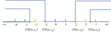
Figure 1: Interval example

III-C Candidate Values for Operations

Since assigning a variable $x$ to any value in an equi-make interval would satisfy the same amount of falsified clauses, after choosing an equi-make interval, we can consider more values in the interval as the option for the future value of operation, rather than only the threshold.

The motivation for the candidate future values is based on the following 3 intuitions: First, we have to restrict the value in the given interval. Moreover, we hope the denominator of corresponding value to be relatively small, in order to avoid exploring complex search space as will be explained in the next section. Finally, the value should be easy to calculate, in order to improve the efficiency of algorithm.

In this work, we only consider the intervals with a positive make value, and thus the interval $(UB^{n},LB^{m})$ is omitted. Thus, the interval for consideration is of the form $(UB^{i-1}(x),UB^{i}(x)]$ or $[LB^{i}(x),LB^{i-1}(x))$. For such an interval, we consider the following values for the operation:

• Assign $x$ to the threshold $UB^{i}(x)$ or $LB^{i}(x)$.

• Assign $x$ to the median of the interval, that is $(UB^{i-1}(x)+UB^{i}(x))/2$ or $(LB^{i}(x)+LB^{i-1}(x))/2$ (when one of the bounds is $\infty$ or $-\infty$, the median will not be considered).

• if there are integers in the interval $(UB^{i-1}(x),UB^{i}(x))$ or the interval $(LB^{i}(x)$, $LB^{i-1}(x))$, assign $x$ to the largest or smallest integer in the respective open interval; Otherwise, suppose that the open interval can be written as $(\frac{a}{b},\frac{c}{d})$, then assign $x$ to $\frac{a+c}{b+d}$.

The first option is the same as critical move, and thus critical move can be regarded as a special case of our interval-based operator. The second option is a simple choice among intervals. The third option aims to find a rational value limited in the open interval with small denominator, and it is easy to calculate.

Note that it is difficult and even even impractical to compute the operations leading to the largest local decrease in the score, based on the following reasons: An operation consists of the variable to modify and the future value to assign. However, the variable can be assigned with arbitrary real number, which is inexhaustible. Although this can be reduced to enumerable intervals, it is still too time-consuming to enumerate all possible operations. Moreover, a literal $\ell$ contains different variables, and changing one such variable would affect all other literals (not only $\ell$) containing the variable. Thus, to calculate the score of an operation, we need to go through all literals containing the variable to modify, which is time-consuming. These two reasons make it a very time-consuming procedure to compute such an operation leading to the largest local decrease in the score.

Thus, our algorithm does not tempt to compute such an operation, but chooses an operation with good score from sampled candidate operations with those candidate values. In the future work, we will further enrich the sampled candidate values by considering more random values with small denominator in the interval.

IV A Tie-breaking Mechanism

We notice that there often exist different operations with the same best $score$ during local search, and thus tie-breaking is also important to guide the search.

To confirm our observation, we conduct a pre-experiment on 100 randomly selected instances. On each instance, we execute a simple local search algorithm which selects an operation with the best $score$ for 10000 iterations, and we count the number of steps where $k$ operations with the same best $score$ are found, denoted as $step(k)$.

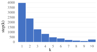
Figure 2: Average $step(k)$ distribution

As shown in Fig. 2, the steps where more than one operations have the same best $score$ take up 61.2% of the total steps. Thus, a tie-breaking heuristic is required to further distinguish these operations with same best $score$.

First, we consider that assigning real-valued variable to values with large denominator can lead the algorithm to a more complex search space where variables are assigned to real number with extremely large denominators, leading to more complicated computation and possible errors, because the local search solver needs to perform factorization of large numbers and numerical approximation to handle these values during the iteration. Thus, we prefer operations that assign variable to a value with a small denominator.

Moreover, we consider that assigning variables to values with large absolute value can lead to the assignment with an extraordinarily large value, deviating the algorithm from finding a possible solution. Thus, we prefer operations assigning variables to values with small absolute value.

Based on the above observation and intuition, we propose a selection rule for picking operations, described as follows.

Selection Rules: Select the operation with the greatest $score$, breaking ties by preferring the one assigning the corresponding variable to a value with the smallest denominator. Further ties are broken by picking the operation assigning the variable with the smallest absolute value.

V LocalSMT(RA) Algorithm

Our local search algorithm adopts a two-mode framework, which switches between Real mode and Boolean mode. This framework has been used in the local search algorithm LS-LIA for integer arithmetic theories [34].

V-A Local search Framework

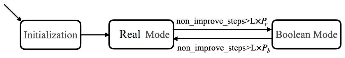
Figure 3: An SMT Local Search Framework

LocalSMT(RA) is running a local search algorithm starting from an arbitrary model with all real-value variables assigned to 0 and all Boolean variables assigned to false. As depicted in Fig. 3, after the initialization, the algorithm switches between Real mode and Boolean mode. In each mode, an operation on a variable of the corresponding data type is selected to modify the current solution. The two modes switches between each other when the number of non-improving steps (denoted as $non\_improve\_steps$) of the current mode reaches a threshold. $non\_improve\_steps$ is increased by one when the algorithm fails to find a better solution, otherwise, it is reset as 0. The threshold is set to $L\times P_{b}$ for the Boolean mode and $L\times P_{r}$ for the Real mode, where $P_{b}$ and $P_{r}$ denote the proportion of Boolean and real-variable literals to all literals in falsified clauses, and $L$ is a parameter.

V-B Local Search in Real and Boolean Mode

The algorithm for the Real mode of LocalSMT(RA) is described in Algorithm 1: if the current assignment $\alpha$ satisfies the given formula $F$, then the solution is found (Line 2). The algorithm tries to find a decreasing interval-based operation according to the Selection Rule (Line 3–4).

If there exists no such decreasing operation, this is an indication that the algorithm falls into the local optimum. We first update the clause weights according to the probabilistic version of the Pure Additive Weighting Scheme (PAWS) [39, 30] (Line 6), and then randomly sample $K$ interval-based operations into the set $Set_{op}$ (Line 7), where $K$ is a relatively small parameter. The best operation is picked according to Selection Rules among $Set_{op}$ (Line 8). Note that since the interval-based operation can satisfy at least one clause, picking the best one among few randomly sampled interval-based operation can be regarded as a diversification operation.

The probabilistic version of the PAWS scheme works as follows. In the beginning, the weight of each clause is initialized as 1. During the local search process, with probability $1-sp$, the weight of each falsified clause is increased by one, and with probability $sp$, for each satisfied clause whose weight is greater than 1, the weight is decreased by one.

As for the Boolean mode focusing on the subformula consisting of Boolean variables, LocalSMT(RA) works in the same way as the Boolean mode of LS-LIA. By putting the Boolean mode and the Real mode together, we propose our local search algorithm for SMT(RA) denoted as LocalSMT(RA).

Input: formula $F$

Output: A satisfying assignment $\alpha$ of $F$, or “UNKNOWN”

1 while non_impr_steps $<L\times P_{r}$ do

2       if $\alpha$ satisfies $F$ then return $\alpha$;

3       if $\exists$ decreasing interval-based operation then

4             $op:=$ such an operation selected according to Selection Rules;

5            

6      

7       else

8             update clause weights according to the PAWS scheme;

9             randomly sample $K$ interval-based operations into the set $Set_{op}$;

10             $op:=$ the best operation among $Set_{op}$ picked by Selection Rules;

11            

12      $\alpha:=\alpha$ with $op$ performed;

13      

14return “UNKNOWN”;

15

Algorithm 1 Real Mode of LocalSMT(RA)

VI Experiments

We conducted experiments to evaluate LocalSMT(RA) on 2 benchmark sets from SMT-LIB, and compare it with state-of-the-art SMT solvers and local search solvers. Moreover, ablation experiments are conducted to analyze the effectiveness of the proposed strategies.

VI-A Experiment Preliminaries

Implementation: LocalSMT(RA) is implemented in C++ and compiled by g++ with ’-O3’ option. There are 3 parameters in LS-LRA: $L$ for switching phases, $K$ for the number of sampled operation and $sp$ (the smoothing probability) for the PAWS scheme. The parameters are tuned according to suggestions from the literature [34, 30] and our preliminary experiments on 20% sampled instances. Preliminary experiments show that LocalSMT(RA) is not sensitive to the parameter setting in a considerable range. Parameters are set as follows: $L=20$, $K=3$, $sp=0.0003$ for all benchmarks. In our implementation, to escape from local optimum, LocalSMT(RA) restarts every 500000 iterations. We use a fixed value for the infinitesimal real number $\delta$, which is $min(\frac{1}{256},\frac{1}{c_{max}})$, where $c_{max}$ denotes the maximum absolute value of coefficients in the formula.

Note that in contrast to previous local search for for SMT on Linear Integer Arithmetic [34], our solver is able to handle arbitrary Boolean structure of formulas, including “ite” operator, by using the Tseitin encoding [40].

Although any formula with high exponents can be rewritten as multi-linear formula by introducing fresh variables (for example, $x^{2}>4$ can be rewritten as $(x=y)\wedge(x*y>4)$), however, in that case, we cannot efficiently find the correct feasible solution of $x$ because of the relationship of both variables. In our implementation, we simplify the formula by eliminating equations in form of $x=(a*y)$, where $x$ and $y$ are real-value variables and $a$ is coefficient. Specifically, we will replace $x$ with $(a*y)$, and after simplifying, we only reserve those instances which are still multi-linear.

Competitors: In the context of SMT(LRA), we compare LocalSMT(RA) with the top 4 state-of-the-art SMT solvers according to SMT-COMP 2022, namely OpenSMT (version 2.4.2) , Yices2 (version 2.6.2) , cvc5 (version 1.0.0) , and Z3 (version 4.8.17) . While in the context of SMT(NRA), the top 4 competitors are as follows, cvc5 (version 1.0.0), Yices2 (version 2.6.2), Z3 (version 4.8.17) and SMT-RAT-MCSAT (version 22.06) . The binaries of all competitors are downloaded from their websites. Note that portfolio and derived solvers are excluded.

Benchmarks: Experiments are carried out on 2 benchmark sets from SMT-LIB.

• SMTLIB-LRA: The benchmark set contains SMT(LRA) instances from SMT-LIB. As LocalSMT(RA) is an incomplete solver, UNSAT instances are excluded, resulting in a benchmark with 1044 unknown and satisfiable instances.

• SMTLIB-MRA: The benchmark set contains SMT(NRA) instances with multi-linear atomic constraints from SMT-LIB. UNSAT instances are also excluded, resulting in a benchmark with 979 unknown and satisfiable instances.

Experiment Setup: All experiments are carried out on a server with AMD EPYC 7763 64-Core 2.45GHz and 2048G RAM under the system Ubuntu 20.04.4. Each solver is executed once with a cutoff time of 1200 seconds (as in the SMT-COMP) for each instance in both benchmark sets, as they contain sufficient instances (1044 for SMTLIB-LRA and 979 for SMTLIB-MRA). We compare the number of instances where an algorithm finds a model (“#solved”), as well as the run time. Bold values in table emphasize the solver with greatest “#solved”.

VI-B Results on SMTLIB-LRA Benchmark

VI-B1 Comparison with DPLL(T) solvers

As shown in Table I, LocalSMT(RA) can solve 900 out of 1044 instances, which is competitive but still cannot rival its competitors. We also perform a runtime comparison between LocalSMT(RA) and each competitor on instances from SMTLIB-LRA in Fig 4, which shows that LocalSMT(RA) is complementary to the competitors.

One explanation for the fact that LocalSMT(RA) cannot rival its DPLL(T) competitors is that 54.5% of the instances in SMTLIB-LRA contain Boolean variables, while the Boolean mode of LocalSMT(RA) is not good at exploiting the relations among Boolean variables, similar to previous local search for SMT on Linear Integer Arithmetic [34]. Another possible reason accounting for the poor performance of LocalSMT(RA) on this benchmark set is that our algorithm is not complete in the sense of probabilistically approximately complete (PAC), because the candidate value selection of interval-based operation can miss the possible satisfying solution where the values of variables are not considered.

TABLE I: Results on instances from SMTLIB-LRA

	#inst	cvc5	Yices	Z3	OpenSMT	LocalSMT(RA)
2017-Heizmann	8	4	3	4	4	7
2019-ezsmt	84	61	61	53	62	35
check	1	1	1	1	1	1
DTP-Scheduling	91	91	91	91	91	91
LassoRanker	271	232	265	256	262	240
latendresse	16	9	12	1	10	0
meti-tarski	338	338	338	338	338	338
miplib	22	14	15	15	15	4
sal	11	11	11	11	11	11
sc	108	108	108	108	108	108
TM	24	24	24	24	24	11
tropical-matrix	10	1	6	4	6	0
tta	24	24	24	24	24	24
uart	36	36	36	36	36	30
Total	1044	954	995	966	992	900

(a) Comparing with cvc5

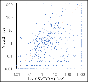
(b) Comparing with Yices2

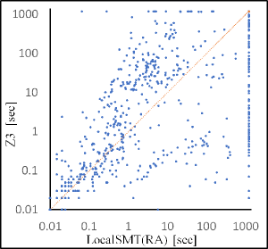
(c) Comparing with Z3

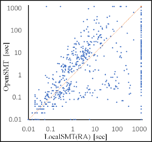
(d) Comparing with OpenSMT

Figure 4: Run time comparison on instances from SMTLIB-LRA

VI-B2 Comparison with Local Search Solvers

We compare LocalSMT(RA) with a previous local search solver dedicated for SMT(LRA) [33], called WalkSMT. The best two configurations of WalkSMT, namely “WalkSMT UBCSAT” and “WalkSMT UBCSAT++”, are adopted for comparison. Since WalkSMT only supports the earlier version of SMT-LIB standard, which has been deprecated, we perform experiments using the same experiment setup in their paper [33], where the cutoff is set as 600s, and we compare with the result presented in the original paper. The results are shown in Table II, indicating that LocalSMT(RA) can significantly outperform both configurations of WalkSMT, especially on the “sc” type.

TABLE II: Comparison with WalkSMT on instances from SMTLIB-LRA

	sc	uart	sal	TM	tta	miplib	Total
#inst	108	36	11	24	24	22	225
WalkSMT UBCSAT	78	35	10	14	9	3	149
WalkSMT UBCSAT++	63	14	8	19	10	2	116
LocalSMT(RA)	106	29	8	9	24	3	179

VI-C Results on SMTLIB-MRA Benchmark

LocalSMT(RA) can solve more multi-linear instances than all competitors on this benchmark set (solving 891 out of 979 instances), which is shown in Table III. Moreover, LocalSMT(RA) can uniquely solve 28 instances in this benchmark set. The time comparison between LocalSMT(RA) and its competitors is shown in Fig 5, confirming that LocalSMT(RA) is more efficient than all competitors in SMTLIB-MRA. As shown in Table IV, LocalSMT(RA) shows better performance with smaller cutoff. Specifically, LocalSMT(RA) can solve 138, 122 and 99 more instances than the best of competitors respectively with the cutoff of 1s, 5s, and 10s.

LocalSMT(RA) works particularly well on instances from “zankl” and “UltimateAutomizer” type, which are industrial instances generated in the context of software verification. On these types, LocalSMT(RA) can solve all instances, outperforming all the competitors. Moreover, LocalSMT(RA) can exclusively solve 13 instances from “20170501-Heizmann” type, which implements a constraint-based synthesis of invariants[41].

The explanation for the superiority of LocalSMT(RA) on SMTLIB-MRA are as follows. In contrast to LRA, the theory solver for NRA constraints requires complex calculation, which reduces the performance of these competitors, while LocalSMT(RA) can trivially determine the operations in multi-linear constraints, and thus LocalSMT(RA) can efficiently explore the search space. Moreover, In SMTLIB-MRA benchmarks, 3.4% instances have Boolean variables. In contrast to SMTLIB-LRA, whose counterpart is 54.5%, SMTLIB-MRA has simpler Boolean structures.

TABLE III: Results on instances from SMTLIB-MRA

	#inst	cvc5	Yices	Z3	SMT-RAT	LocalSMT(RA)
20170501-Heizmann	51	1	0	4	0	17
20180501-Economics	28	28	28	28	28	28
2019-ezsmt	32	31	32	32	21	28
20220314-Uncu	12	12	12	12	12	12
LassoRanker	347	312	124	199	0	297
meti-tarski	423	423	423	423	423	423
UltimateAutomizer	48	34	39	46	18	48
zankl	38	24	25	28	30	38
Total	979	865	683	772	532	891

TABLE IV: Results on instances from SMTLIB-MRA with different cutoff

Cutoff		cvc5	Yices	Z3	SMT-RAT	LocalSMT(RA)
1s		535	567	595	495	733
5s		607	609	674	507	796
10s		649	623	714	508	813

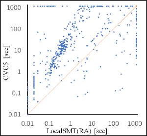
(a) Comparing with cvc5

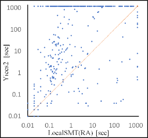
(b) Comparing with Yices2

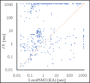
(c) Comparing with Z3

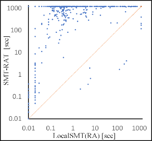
(d) Comparing with SMT-RAT

Figure 5: Run time comparison on instances from SMTLIB-MRA

VI-D Effectiveness of Proposed strategies

To analyze the effectiveness of the strategies in LocalSMT(RA), we modify LocalSMT(RA) to obtain 3 alternative versions as follows.

• To analyze the effectiveness of interval-based operator, LocalSMT(RA) is modified by replacing the operator with traditional $cm$ operator, leading to the version $v\_{cm}$.

• To analyze the effectiveness of the tie-breaking mechanism, we modify LocalSMT(RA) by evaluating operation based on $score$ without considering the Selection Rules, that is to randomly pick one operation with greatest $score$, leading to the version $v\_{score}$.

• We also implement a plain version which adopts neither interval-based operator nor tie-breaking mechanism, denoted as $v\_{plain}$.

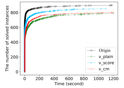
(a) Comparison on SMTLIB-LRA

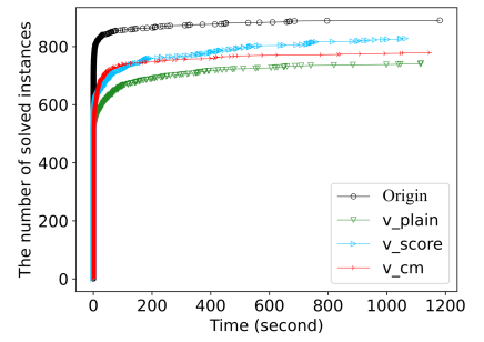
(b) Comparison on SMTLIB-MRA

Figure 6: Run time distribution comparison

The original version of LocalSMT(RA), denoted as $Origin$, is compared with these modified versions on both benchmarks. The runtime distribution of LocalSMT(RA) and its modified versions is presented in Fig. 6, which confirms the effectiveness of our proposed strategies.

VII Conclusion and Future Work

In this paper, we propose the first local search algorithm for SMT on Real Arithmetic based on the following novel ideas. First, the interval-based operation is proposed to enrich the traditional critical move operator, by considering the interval information. Moreover, a tie-breaking mechanism is proposed to distinguish operations with same best $score$. Experiments on SMT-LIB show that our solver is competitive and complementary with state-of-the-art SMT solvers, especially for those multi-linear instances.

The future direction is to extend LocalSMT(RA) to support all SMT(NRA) instances and deeply combine our local search algorithm with the DPLL(T) SMT solver, resulting in a hybrid solver that can make the most of respective advantages. Moreover, we will enrich the sampled candidate values of interval-based operation by considering more random values with small denominator.

VIII Acknowledgements

This work is supported by NSFC Grant 62122078.

References

- [1] S. Lahiri and S. Qadeer, “Back to the future: revisiting precise program verification using smt solvers,” ACM SIGPLAN Notices, vol. 43, no. 1, pp. 171–182, 2008.
- [2] N. S. Bjørner, K. L. McMillan, and A. Rybalchenko, “Program verification as satisfiability modulo theories.” SMT@ IJCAR, vol. 20, pp. 3–11, 2012.
- [3] R. Baldoni, E. Coppa, D. C. D’elia, C. Demetrescu, and I. Finocchi, “A survey of symbolic execution techniques,” ACM Computing Surveys (CSUR), vol. 51, no. 3, pp. 1–39, 2018.
- [4] J. Peleska, E. Vorobev, and F. Lapschies, “Automated test case generation with smt-solving and abstract interpretation,” in NASA Formal Methods: Third International Symposium, NFM 2011, Pasadena, CA, USA, April 18-20, 2011. Proceedings 3. Springer, 2011, pp. 298–312.
- [5] R. Sebastiani, “Lazy satisfiability modulo theories,” JSAT, vol. 3, no. 3-4, pp. 141–224, 2007.
- [6] C. Barrett and C. Tinelli, “Satisfiability modulo theories,” in Handbook of model checking. Springer, 2018, pp. 305–343.
- [7] R. Nieuwenhuis, A. Oliveras, and C. Tinelli, “Solving sat and sat modulo theories: From an abstract davis–putnam–logemann–loveland procedure to dpll (t),” Journal of the ACM, vol. 53, no. 6, pp. 937–977, 2006.
- [8] L. De Moura and N. Bjørner, “Z3: An efficient smt solver,” in Tools and Algorithms for the Construction and Analysis of Systems: 14th International Conference, TACAS 2008, Held as Part of the Joint European Conferences on Theory and Practice of Software, ETAPS 2008, Budapest, Hungary, March 29-April 6, 2008. Proceedings 14. Springer, 2008, pp. 337–340.
- [9] B. Dutertre, “Yices 2.2,” in Computer Aided Verification: 26th International Conference, CAV 2014, Held as Part of the Vienna Summer of Logic, VSL 2014, Vienna, Austria, July 18-22, 2014. Proceedings 26. Springer, 2014, pp. 737–744.
- [10] F. Corzilius, U. Loup, S. Junges, and E. Ábrahám, “Smt-rat: An smt-compliant nonlinear real arithmetic toolbox: (tool presentation),” in Theory and Applications of Satisfiability Testing–SAT 2012: 15th International Conference, Trento, Italy, June 17-20, 2012. Proceedings 15. Springer, 2012, pp. 442–448.
- [11] H. Barbosa, C. Barrett, M. Brain, G. Kremer, H. Lachnitt, M. Mann, A. Mohamed, M. Mohamed, A. Niemetz, A. Nötzli et al., “cvc5: A versatile and industrial-strength smt solver,” in Tools and Algorithms for the Construction and Analysis of Systems: 28th International Conference, TACAS 2022, Held as Part of the European Joint Conferences on Theory and Practice of Software, ETAPS 2022, Munich, Germany, April 2–7, 2022, Proceedings, Part I. Springer, 2022, pp. 415–442.
- [12] R. Bruttomesso, E. Pek, N. Sharygina, and A. Tsitovich, “The opensmt solver.” in TACAS, vol. 6015. Springer, 2010, pp. 150–153.
- [13] A. Cimatti, A. Griggio, B. J. Schaafsma, and R. Sebastiani, “The mathsat5 smt solver,” in Tools and Algorithms for the Construction and Analysis of Systems: 19th International Conference, TACAS 2013, Held as Part of the European Joint Conferences on Theory and Practice of Software, ETAPS 2013, Rome, Italy, March 16-24, 2013. Proceedings 19. Springer, 2013, pp. 93–107.
- [14] B. Dutertre and L. De Moura, “A fast linear-arithmetic solver for dpll (t),” in Computer Aided Verification: 18th International Conference, CAV 2006, Seattle, WA, USA, August 17-20, 2006. Proceedings 18. Springer, 2006, pp. 81–94.
- [15] N. Bjørner, “Linear quantifier elimination as an abstract decision procedure,” in Automated Reasoning: 5th International Joint Conference, IJCAR 2010, Edinburgh, UK, July 16-19, 2010. Proceedings 5. Springer, 2010, pp. 316–330.
- [16] G. E. Collins, “Quantifier elimination for real closed fields by cylindrical algebraic decompostion,” in Automata Theory and Formal Languages: 2nd GI Conference Kaiserslautern, May 20–23, 1975. Springer, 1975, pp. 134–183.
- [17] U. Loup, K. Scheibler, F. Corzilius, E. Ábrahám, and B. Becker, “A symbiosis of interval constraint propagation and cylindrical algebraic decomposition,” in Automated Deduction–CADE-24: 24th International Conference on Automated Deduction, Lake Placid, NY, USA, June 9-14, 2013. Proceedings 24. Springer, 2013, pp. 193–207.
- [18] S. Junges, U. Loup, F. Corzilius, and E. Ábrahám, “On gröbner bases in the context of satisfiability-modulo-theories solving over the real numbers,” in Algebraic Informatics: 5th International Conference, CAI 2013, Porquerolles, France, September 3-6, 2013. Proceedings 5. Springer, 2013, pp. 186–198.
- [19] S. Basu, “Algorithms in real algebraic geometry: a survey,” arXiv preprint arXiv:1409.1534, 2014.
- [20] F. Corzilius and E. Ábrahám, “Virtual substitution for smt-solving,” in Fundamentals of Computation Theory: 18th International Symposium, FCT 2011, Oslo, Norway, August 22-25, 2011. Proceedings 18. Springer, 2011, pp. 360–371.
- [21] V. Weispfenning, “Quantifier elimination for real algebra—the quadratic case and beyond,” Applicable Algebra in Engineering, Communication and Computing, vol. 8, pp. 85–101, 1997.
- [22] P. Van Hentenryck, D. McAllester, and D. Kapur, “Solving polynomial systems using a branch and prune approach,” SIAM Journal on Numerical Analysis, vol. 34, no. 2, pp. 797–827, 1997.
- [23] S. Gao, S. Kong, and E. M. Clarke, “dreal: An smt solver for nonlinear theories over the reals,” in Automated Deduction–CADE-24: 24th International Conference on Automated Deduction, Lake Placid, NY, USA, June 9-14, 2013. Proceedings 24. Springer, 2013, pp. 208–214.
- [24] S. Schupp, E. Ábrahám, P. Rossmanith, and D.-I. U. Loup, “Interval constraint propagation in smt compliant decision procedures,” Master’s thesis, RWTH Aachen, 2013.
- [25] D. Jovanovic, C. Barrett, and L. De Moura, “The design and implementation of the model constructing satisfiability calculus,” in 2013 Formal Methods in Computer-Aided Design. IEEE, 2013, pp. 173–180.
- [26] D. Jovanović and L. De Moura, “Solving non-linear arithmetic,” ACM Communications in Computer Algebra, vol. 46, no. 3/4, pp. 104–105, 2013.
- [27] H. H. Hoos and T. Stützle, Stochastic local search: Foundations and applications, 2004.
- [28] C. M. Li and Y. Li, “Satisfying versus falsifying in local search for satisfiability,” in Proc. of SAT 2012, 2012, pp. 477–478.
- [29] A. Balint and U. Schöning, “Choosing probability distributions for stochastic local search and the role of make versus break,” in Proc. of SAT 2012, 2012, pp. 16–29.
- [30] S. Cai and K. Su, “Local search for boolean satisfiability with configuration checking and subscore,” Artificial Intelligence, vol. 204, pp. 75–98, 2013.
- [31] S. Cai, C. Luo, and K. Su, “CCAnr: A configuration checking based local search solver for non-random satisfiability,” in Proc. of SAT 2015, 2015, pp. 1–8.
- [32] A. Biere, “Splatz, Lingeling, Plingeling, Treengeling, YalSAT entering the SAT competition 2016,” Proc. of SAT Competition 2016, pp. 44–45, 2016.
- [33] A. Griggio, Q.-S. Phan, R. Sebastiani, and S. Tomasi, “Stochastic local search for smt: combining theory solvers with walksat,” in International Symposium on Frontiers of Combining Systems. Springer, 2011, pp. 163–178.
- [34] S. Cai, B. Li, and X. Zhang, “Local search for smt on linear integer arithmetic,” in International Conference on Computer Aided Verification. Springer, 2022, pp. 227–248.
- [35] ——, “Local search for satisfiability modulo integer arithmetic theories,” ACM Transactions on Computational Logic, 2022.
- [36] A. Niemetz, M. Preiner, and A. Biere, “Propagation based local search for bit-precise reasoning,” Formal Methods Syst. Des., vol. 51, no. 3, pp. 608–636, 2017. [Online]. Available: https://doi.org/10.1007/s10703-017-0295-6
- [37] A. Niemetz and M. Preiner, “Ternary propagation-based local search for more bit-precise reasoning,” in 2020 Formal Methods in Computer Aided Design, FMCAD 2020, Haifa, Israel, September 21-24, 2020. IEEE, 2020, pp. 214–224. [Online]. Available: https://doi.org/10.34727/2020/isbn.978-3-85448-042-6_29
- [38] A. Fröhlich, A. Biere, C. M. Wintersteiger, and Y. Hamadi, “Stochastic local search for satisfiability modulo theories,” in Proceedings of the Twenty-Ninth AAAI Conference on Artificial Intelligence, January 25-30, 2015, Austin, Texas, USA, B. Bonet and S. Koenig, Eds. AAAI Press, 2015, pp. 1136–1143. [Online]. Available: http://www.aaai.org/ocs/index.php/AAAI/AAAI15/paper/view/9896
- [39] J. Thornton, D. N. Pham, S. Bain, and V. F. Jr., “Additive versus multiplicative clause weighting for SAT,” in Proc. of AAAI 2004, 2004, pp. 191–196.
- [40] S. D. Prestwich, “Cnf encodings.” Handbook of satisfiability, vol. 185, pp. 75–97, 2009.
- [41] M. A. Colón, S. Sankaranarayanan, and H. B. Sipma, “Linear invariant generation using non-linear constraint solving,” in International Conference on Computer Aided Verification. Springer, 2003, pp. 420–432.