Superconductivity Studied by Solving Ab Initio Low-Energy Effective Hamiltonians for Carrier Doped CaCuO₂, Bi₂Sr₂CuO₆, Bi₂Sr₂CaCu₂O₈, and HgBa₂CuO₄

Abstract

Understanding the materials dependence together with the universal controlling parameter of superconductivity (SC) in copper oxide superconductors is one of the major challenges in condensed matter physics. Here, we numerically analyze SC by using ab initio low-energy effective Hamiltonians consisting of the antibonding (AB) combination of Cu $3d_{x^{2}-y^{2}}$ and O $2p_{\sigma}$ orbitals without adjustable parameters. We have performed the state-of-the-art variational Monte Carlo calculations for the four carrier doped cuprates with diverse experimental optimal SC critical temperature $T_{c}^{\rm opt}$: CaCuO₂ ($T_{c}^{\rm opt}\sim 110$ K), Bi₂Sr₂CuO₆ ($T_{c}^{\rm opt}\sim 10$-$40$ K), Bi₂Sr₂CaCu₂O₈ ($T_{c}^{\rm opt}\sim 85$-$100$ K), and HgBa₂CuO₄ ($T_{c}^{\rm opt}\sim 90$ K). Materials and hole doping concentration ($\delta$) dependencies of the SC order parameter $F_{\rm SC}$ and the competition with spin and charge orders show essential and quantitative agreement with the available experiments on the four materials in the following points: (1) In a wide range $0.05\leq\delta\leq 0.25$, the ground state is commonly the uniform SC state, which is severely competing with the charge, spin stripe and antiferromagnetic (AFM) states. (2) $F_{\rm SC}$ at the optimum doping shows amplitude consistent with the superfluid density measured in the muon spin resonance ($\mu$SR) and its dome structure found in $\delta$ dependence shows consistency with that of the SC gap in the tunneling and photoemission measurements. Based on the confirmed materials dependence, we further find insights into the universal SC mechanism: (I) $F_{\rm SC}$ increases with the ratio $U/|t_{1}|$ within the available realistic materials, indicating that $U/|t_{1}|$ is the principal component controlling the strength of the SC in the real materials dependence. Here, $U$ and $t_{1}$ are the on-site Coulomb repulsion and the nearest neighbor hopping, respectively, in the ab initio Hamiltonians. (II) A universal scaling $T_{c}^{\rm opt}\sim 0.16\lvert t_{1}\rvert F_{\rm SC}$ holds. (III) SC is enhanced and optimized if $U$ is increased beyond the real available materials, and it is further enhanced when the off-site interaction is reduced, while the presence of the off-site interaction is important to make the SC ground state against other competing states. The present findings provide useful clues for the design of new SC materials with even higher $T_{c}^{\rm opt}$.

I Introduction

The mechanism and origin of the large superconducting (SC) gap, high superfluid density, and high critical temperatures $T_{c}$ observed in high-$T_{c}$ superconductors, such as copper oxides, remain a central challenge in condensed matter physics. In these copper oxides, the $d$-wave SC state is severely competing with other orders, such as spin and charge stripes or antiferromagnetic (AFM) states, and the observed $T_{c}$ widely ranges from above $130\,\text{K}$ to below $10\,\text{K}$. Understanding and reproducing these diverse phenomena without relying on adjustable parameters is hence desirable, especially when clarifying their origin. When ab initio calculations are able to reproduce systematic materials dependence quantitatively by solely relying on their crystal structures, it provides us with valuable insight into the universal mechanism behind and into the principal components for the enhancement of SC beyond existing materials.

Many studies have suggested severe competitions of the SC with charge/spin stripe and AFM states theoretically based on simplified Hubbard-like or $t$-$J$ Hamiltonians as models of the cuprate superconductors [1, 2, 3, 4, 5, 6, 7, 8]. A positive correlation between $U$ and $T_{c}$ or SC tendency was also pointed out by taking $U$ as an adjustable parameter in the Hubbard type Hamiltonians [9]. However, ab initio studies without adjustable parameters are few and it is not clear whether the diversity of the materials dependence can be accounted for. There still exists a limited number of ab initio studies: The phase diagram including the SC phase was reproduced by solving the ab initio Hamiltonian for a particular case of Hg compound [10]. Ab initio Hamiltonians were derived by Nilsson et al. for several cuprate compounds, which reported an empirical observation without solving the Hamiltonians that the experimental optimal $T_{c}$ is generally higher for larger $U/|t|$ in their parameters [11, 12]. The relation of the charge transfer energy to $T_{c}$ was also pointed out [13, 14]. Aside from the cuprates, there exist some ab initio studies on strong-coupling superconducting materials such as the iron-based superconductors [15], fullerene [16], and nickelates [17] to discuss the superconducting properties. However, to our knowledge, there exist no systematic studies on the SC properties by solving solely ab initio Hamiltonians without adjustable parameters with the help of accurate many-body solvers to reveal the origin of the diverse materials dependence, especially for the challenging cuprates. Unless reproducing the materials dependent properties quantitatively, the universal mechanism would also not be able to be identified confidently either.

In this paper we show properties of typical cuprate superconductors calculated by solving the ab initio Hamiltonians of four families of materials, namely carrier doped CaCuO₂, HgBa₂CuO₄ (abbreviated as Hg1201 hereafter), Bi₂Sr₂CuO₆ (Bi2201 hereafter), and Bi₂Sr₂CaCu₂O₈ (Bi2212 hereafter) [12], by applying a state-of-the-art quantum many-body solver based on the variational Monte Carlo (VMC) algorithm [18, 19], including the combination with neural network [20, 21] elaborated from earlier variational algorithms [22, 23, 24, 25]. It is experimentally known that the optimum critical temperature $T_{c}^{\rm opt}$ is realized at around $\delta=0.1$-0.15 [26, 27] for doped CaCuO₂ ($T_{c}^{\rm opt}\sim$ 110K) and Hg1201 ($T_{c}^{\rm opt}\sim$ 90K), and at around $\delta=0.15$-0.25 [28, 29, 30] for doped Bi2212 ($T_{c}^{\rm opt}\sim$ 85-100K) and Bi2201 ($T_{c}^{\rm opt}\sim$ 10-40K). We elucidate that similarity and diversity among the four families, especially the amplitude of the SC order parameters and $T_{c}^{\rm opt}$ in the experiments are accounted for by using the present ab initio results, which provides us with insights into the materials dependence and the universal mechanism:

We emphasize that our ab initio analyses contain essential differences from most of the Hubbard models studies. One important difference is the presence of the realistic off-site interactions. We will clarify that this crucially stabilizes the charge uniform SC state without clear stripe long-range order.

The dominance of the SC for all the four families is successfully demonstrated. In addition, the $\delta$ dependence of $F_{\rm SC}$ has a dome structure with the peak at $\delta\sim 0.05$-$0.1$ consistently with the experimental indications. On the other hand, the dome peak of $T_{c}$ appears at larger $\delta>0.1$ in the experiment. This shift from the dome peak of $F_{\rm SC}$ is understood from the decreasing renormalization factor with decreasing doping, which does not affect $F_{\rm SC}$ but $T_{c}$.

Although $T_{c}^{\rm opt}$ has a variety among these four families, we show universally that (I) the higher SC order parameter $F_{\rm SC}$ at the optimal doping basically results from a larger ratio $U/|t_{1}|$, where $U$ is the on-site repulsive Coulomb interaction and $t_{1}$ is the nearest neighbor hopping in our ab initio parameters of single-band effective Hamiltonian for the AB orbital of strongly hybridized Cu $3d_{x^{2}-y^{2}}$ and O $2p_{\sigma}$ orbitals. Furthermore, we show that (II) $T_{c}^{\rm opt}$ is determined by the scaling $T_{c}^{\rm opt}\sim 0.16\lvert t_{1}\rvert F_{\rm SC}$.

The $\delta$ dependence of the local energy suggests a universal superconducting mechanism: Though the bare interaction is strongly repulsive, the Mottness converts it to the strong effective attraction required for the Cooper pairing.

Despite monotonic increase of $F_{\rm SC}$ with $U/|t_{1}|$ within the existing materials, we further show that (III) larger $U/|t_{1}|$ beyond the ab initio values makes the peak of $F_{\rm SC}$ followed by the reduction. We find that $F_{\rm SC}$ can be roughly 30% more enhanced than the ab initio case when $U$ is 20% increased beyond the ab initio value by preserving the transfer and other off-site interaction parameters. We also show that $F_{\rm SC}$ is further enhanced to as much as the double of the existing material by the additional reduction of the off-site Coulomb interaction. These searches beyond the ab initio parameters for the existing materials offer a guide for future experimental materials design.

This paper is organized as follows. Section II presents the methods and computational details: First, the effective Hamiltonians studied in this paper are summarized in Sec. II.1. Then, we give the numerical methods in Sec. II.2 and define the physical quantities in Sec. II.3. We present in Sec. III the results for each of the four families of compounds. Based on the obtained ab initio results, in Sec. IV, we further explore the direction to enhance and optimize the SC order parameter by controlling the effective interaction parameters beyond the ab initio values, to gain insights into the future materials design. In Sec. V, we discuss our analyses. Summary and conclusion are given in Sec. VI.

II Methods

II.1 Ab initio effective Hamiltonian

Within this paper, we solve the ab initio single-band effective Hamiltonians for CaCuO₂, Hg1201, Bi2201, and Bi2212 as derived in Ref. [12]. It should be noted that the single band is constructed from the AB orbital of strongly hybridized Cu 3$d_{x^{2}-y^{2}}$ and O 2$p_{\sigma}$ orbitals and not from the atomic single orbital of Cu 3$d_{x^{2}-y^{2}}$. This is justified by very large hybridization gap of the AB and bonding (B) or nonbonding (NB) orbitals. See Appendix D of Ref. [12] and the last paragraph of Sec. V in this paper. Here the transfer and interaction parameters are derived at values close to the experimental optimum hole concentration (at 10% doping for CaCuO₂ and Hg1201 and at 20% for the two Bi compounds). This choice is appropriate in this paper, because properties at optimum hole concentration are the central subject. The effective Hamiltonians have the form

$$\mathcal{H} =\mathcal{H}_{\rm kin}+\mathcal{H}_{U}+\mathcal{H}_{V}$$ (1)

with

$$\mathcal{H}_{\rm kin} = \sum_{i,j,\sigma}t_{ij}c^{\dagger}_{i\sigma}c^{\phantom{\dagger}}_{j\sigma},$$

$$\mathcal{H}_{U} = \sum_{i}Un_{i\uparrow}n_{i\downarrow},$$

$$\mathcal{H}_{V} = \frac{1}{2}\sum_{i\neq j}V_{ij}n_{i}n_{j}.$$

Here $i,j$ are the unit cell indices of the maximally localized Wannier function [31, 32] and $c^{\dagger}_{i\sigma}$ ($c^{\phantom{\dagger}}_{i\sigma}$) is the corresponding creation (annihilation) operator of an electron of spin $\sigma$ at the site $i$. The number operator is given by $n_{i}=\sum_{\sigma}n_{i\sigma}$ and $n_{i\sigma}=c^{\dagger}_{i\sigma}c^{\phantom{\dagger}}_{i\sigma}$. Hopping amplitudes $t_{ij}$ in the kinetic energy $\mathcal{H}_{\rm kin}$ depend on the relative coordinate vector $\bm{r}_{i}-\bm{r}_{j}$ by assuming the translational invariance of the crystal structure. The direct effective Coulomb interaction given by $\mathcal{H}_{U}$ is scaled by the on-site interaction $U$, and off-site interaction $\mathcal{H}_{V}$ is the sum over the combination of the site $i$ and $j$, which is proportional to $V_{ij}$. Leading values for all of the four materials are listed in Table 1. For longer ranged part of $t_{ij}$ and $V_{ij}$, see Sec. S1A in Supplemental Material (SM) [33]. Note that the Hamiltonian parameters for Hg1201 in Ref. [12], which we employ, are improved from Ref. [34]. It results in slightly different physical quantities on the quantitative level in the present solution in comparison to Ref. [10].

From four different materials, we learn that the realistic range of available ab initio Hamiltonian parameters is estimated to be $6\lesssim U/|t_{1}|\lesssim 10,0.2\lesssim|t_{2}/t_{1}|\lesssim 0.3,1.2\lesssim|V_{1}/t_{1}|\lesssim 2.0,0.5\lesssim|V_{2}/t_{1}|\lesssim 1.2$ etc. (see also Table 4). In this paper, we investigate whether the diversity of the SC properties can be understood within this range of parameters.

Table 1: Ab initio single-band effective Hamiltonian for CaCuO₂, Hg1201, Bi2212, and Bi2201 taken from Ref. [12]. $U$ is the on-site interaction. The $n$th-neighbor hopping amplitude and Coulomb interaction are denoted as $t_{n}$ and $V_{n}$, respectively. Interlayer hoppings and interactions are neglected here. All values are given in eV.

	$t_{1}$	$t_{2}$	$t_{3}$	$t_{4}$	$t_{5}$
CaCuO2	-0.521	0.132	-0.047	0.008	0.000
Hg1201	-0.544	0.111	-0.043	0.010	0.000
Bi2212	-0.452	0.135	-0.053	-0.001	0.007
Bi2201	-0.527	0.140	-0.042	0.009	-0.007
	$U$	$V_{1}$	$V_{2}$	$V_{3}$	$V_{4}$
CaCuO2	4.221	0.969	0.539	0.380	0.316
Hg1201	3.999	1.002	0.596	0.448	0.389
Bi2212	4.226	0.915	0.518	0.366	0.312
Bi2201	4.393	1.030	0.602	0.450	0.395

We note that the effective Hamiltonian parameters in Eq. (1) are restricted to a single CuO₂ layer. However, in the case of multilayer cuprates CaCuO₂ and Bi2212, the distance between CuO₂ layers is comparable to the cell parameter along $x$ direction, so that interlayer coupling parameters (given in Table 6 in Appendix for Bi2212) also exist in the effective Hamiltonian [12], and its amplitude $V_{n}^{l}\lesssim 0.6$ eV is comparable to that of the intralayer off-site interaction $V_{n}\lesssim 0.9$ eV. This interlayer coupling is ignored in Eq. (1), but potentially plays a role in the SC properties. This role is actually examined in Sec. III.3.1 in the case of Bi2212, which ensures that the SC order parameter $F_{\rm SC}^{\infty}$ (defined later in Sec. II.3) and physical quantities are essentially not affected by the interlayer coupling within the present case of CaCuO₂ and Bi2212 as we discuss in Sec III.3.1. Thus, we restrict to Eq. (1) even in the case of CaCuO₂ and Bi2212. We employ this “single-layer approximation” for all the four materials throughout this paper unless otherwise noted.

II.2 Numerical Methods

We solve the Hamiltonian in Eq. (1) by applying the many-variable variational Monte Carlo (mVMC) method [19, 18] with a trial wave function of the form $\ket{\psi}=\mathcal{P}^{\mathrm{G}}\mathcal{P}^{\mathrm{J}}\mathcal{P}^{\mathrm{dh}}\ket{\phi^{\mathrm{pair}}}$. Here we consider the Gutzwiller factor $\mathcal{P}^{\mathrm{G}}=\exp(-g\sum_{i}n_{i\uparrow}n_{i\downarrow})$ [35], the Jastrow correlation factor $P^{\mathrm{J}}=\exp(\sum_{i<j}\alpha_{ij}n_{i}n_{j})$ [36, 37], the doublon-holon correlation factor $\mathcal{P}^{\mathrm{dh}}=\exp[-\sum_{m=0}^{4}\sum_{\ell=1,2}\alpha^{(\ell)}_{m}\sum_{i}\xi^{(\ell)}_{i(m)}]$ [38], and a generalized pairing wave function of the form $\ket{\phi}^{\mathrm{pair}}=(\sum_{i\sigma,j\sigma^{\prime}}f_{i\sigma,j\sigma^{\prime}}c^{\dagger}_{i\sigma}c^{\dagger}_{j\sigma^{\prime}})^{N_{\mathrm{e}}/2}\ket{0}$. The variational parameters are $g$, $\alpha_{ij}$, $\alpha^{(\ell)}_{m}$, and $f_{i\sigma,j\sigma^{\prime}}$.

We also supplement the mVMC method with the restricted Boltzmann machine (RBM) [20] and the first-order Lanczos step to improve the wave function and also to take the zero limit of the variance extrapolation to improve the estimate by following the variance extrapolation method [39, 40, 41] and by using the simple mVMC, mVMC +Lanczos, and mVMC+RBM results (see Appendices A, B, and Ref. [42] for the detailed procedure.

Competing states with spin and/or charge order or strong fluctuations can be studied by imposing the mean-field order at the initial trial wave function [19]. The correlated metallic state without any symmetry breaking can also be studied by using the ground-state wave function of the noninteracting system as an initial state. These initial states are then relaxed to lower the energy by optimizing the variational parameters. If the competing states exist, the optimization leads to multiple locally stable solutions. The true ground state is determined by comparing the total energy after taking the variance extrapolation described in Appendix B and if possible after careful size extrapolation to see the thermodynamic limit.

The computational details are the following. For all numerical solutions of finite-size lattices subsequently presented in this paper, we assumed the antiperiodic-periodic boundary condition on a $N=L\times L$ square lattice of length $L$, where $N$ is the number of sites on the single-layer system by ignoring the interlayer coupling except for Bi2212. For Bi2212, we examine the two-layer system to examine the effect of interlayer coupling, because a unit cell of Bi2212 contains two layers and the interlayer coupling could play roles in the SC. Within a layer, hoppings and interactions were taken into account up to $t_{9}$ and $V_{9}$, i.e., up to the 2D distance $\bm{R}=(3,3)$ in the unit of the Cu-Cu distance, while contributions smaller than $0.001$ eV were ignored. Unless explicitly mentioned this is applied throughout the whole paper. We concentrate solely on hole doped cases, where the hole doping is given via $\delta=1-N_{e}/N$ and $N_{e}$ is the number of electrons in the system.

II.3 Physical Quantities

The physical quantities discussed in this paper are defined as follows: The total energy per site $E/N=\braket{\mathcal{H}}/N$ is calculated after the variance extrapolation as it is summarized in Appendix B. To see whether the state has spin and charge order, we compute the spin structure factor

$$S_{s}(\bm{q})=\frac{1}{N}\sum_{i,j}\braket{\bm{S}_{i}\cdot\bm{S}_{j}}\mathrm{e}^{\mathrm{i}\bm{q}(\bm{r}_{i}-\bm{r}_{j})}.$$ (2)

and the charge structure factor

$$S_{c}(\bm{q})=\frac{1}{N}\sum_{i,j}\braket{n_{i}n_{j}}\mathrm{e}^{\mathrm{i}\bm{q}(\bm{r}_{i}-\bm{r}_{j})},$$ (3)

where $\bm{S}_{i}=(S_{i}^{x},S_{i}^{y},S_{i}^{z})=\sum_{\sigma,\sigma^{\prime}}c_{i\sigma}^{\dagger}\bm{\sigma}_{\sigma\sigma^{\prime}}c_{i\sigma^{\prime}}/2$ is the spin-1/2 operator and $\bm{\sigma}_{\sigma\sigma^{\prime}}$ is the Pauli matrix $(=(\sigma^{x}_{\sigma\sigma^{\prime}},\sigma^{y}_{\sigma\sigma^{\prime}},\sigma^{z}_{\sigma\sigma^{\prime}})$). The long-range order is determined whether $S_{s}(\bm{q})/N$ or $S_{c}(\bm{q})/N$ remains after taking the limit $N\rightarrow\infty$. The SC long-range order is measured by the $d$-wave SC correlation function

$$P_{d}(\bm{r})=\frac{1}{2N}\sum_{\bm{r}_{i}}\braket{\Delta^{\dagger}_{d}(\bm{r}_{i})\Delta^{\phantom{\dagger}}_{d}(\bm{r}_{i}+\bm{r})+\text{h.c.}}.$$ (4)

Here $\Delta^{\dagger}_{d}(\bm{r}_{i})$ describes the order parameter of the form

$$\Delta^{\phantom{\dagger}}_{d}(\bm{r}_{i})=\frac{1}{\sqrt{2}}\sum_{\bm{r}}f_{d}(\bm{r})(c_{\bm{r}_{i}\uparrow}c_{\bm{r}_{i}+\bm{r}\downarrow}{-}c_{\bm{r}_{i}\downarrow}c_{\bm{r}_{i}+\bm{r}\uparrow}),$$ (5)

where the $d_{x^{2}-y^{2}}$-wave symmetry is included via the form factor

$$f_{d}(\bm{r})=\delta_{r_{y},0}(\delta_{r_{x},1}+\delta_{r_{x},-1})-\delta_{r_{x},0}(\delta_{r_{y},1}+\delta_{r_{y},-1}).$$ (6)

Then, we deduce $P_{d}(\bm{r})$ over the long-range part, as

$$\bar{P}_{d}(L)=\frac{1}{M}\sum_{\sqrt{2}L/4<\lvert\bm{r}\rvert}P_{d}(\bm{r}),$$ (7)

where $\bm{r}=(r_{x},r_{y})$ includes all sites within the square $(-L/2,L/2]^{2}$ and $M$ is the number of lattice points satisfying $\sqrt{2}L/4<\lvert\bm{r}\rvert<\sqrt{2}L/2$. We define the SC order parameter in the thermodynamic limit, $F_{\rm SC}^{\infty}$ by

$$F_{\rm SC}^{\infty} = \lim_{L\rightarrow\infty}F_{\rm SC}(L)=\sqrt{\bar{P}_{d}^{\infty}},$$ (8)

$$F_{\rm SC}(L) \equiv \sqrt{\bar{P}_{d}(L)}$$

$$\bar{P}_{d}^{\infty} = \lim_{L\rightarrow\infty}\bar{P}_{d}(L).$$

III Ab initio results

In this section we present our calculated ab initio results on the four families of compounds. We first analyze the results for doped CaCuO₂ in detail and then compare it with the result of doped Hg1201. Doped Bi2201 and Bi2212 suffer from the experimental uncertainty of the apical oxygen position due to the supermodulation of the crystal structure. Since it generates a variance of the Hamiltonian parameters if one assumes the translational symmetry of the Hamiltonian parameters, we show the properties by indicating this range. All of the four materials show dominance of the $d$-wave SC in the doping concentration dependence and the calculated results reproduce the experimental materials dependence of the strength of SC, which makes it possible to extract the universal properties and systematic trends as well.

III.1 Doped CaCuO₂

Here, we present the results of our calculation for the doped CaCuO₂ in the following order:
(1) $\delta$ dependence of SC properties; in particular, $\bar{P}^{\infty}_{d}$ and the $d$-wave SC order parameter $F^{\infty}_{\rm SC}$. (See the definitions in Sec. II.3.)
(2) Competition between the SC state and other competing states including stripe states.

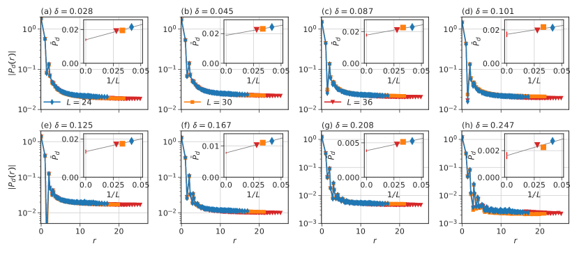
Figure 1: SC correlation function $P_{d}(r)$ for CaCuO₂ at different hole dopings: (a) $\delta=0.028$, (b) $\delta=0.045$, (c) $\delta=0.087$, (d) $\delta=0.101$, (e) $\delta=0.125$ (here $L=28$ instead of $L=30$), (f) $\delta=0.167$, (g) $\delta=0.208$, (h) $\delta=0.247$. In each case, we show $P_{d}(r)$ for the square lattice size $L=24,30,36$. For the same distance $r$ we employ the largest value of correlation. We perform the same procedure in later figures. Inset of each panel: Size extrapolation of $\bar{P}_{d}(L)$ to the thermodynamic limit $\bar{P}_{d}^{\infty}$, whose numerical value is listed in Table 2. The gray line shows the linear approximation. Statistical errors originating from the Monte Carlo sampling are smaller than the symbol size.

III.1.1 Properties of superconducting phase

First, we discuss the $\bm{r}$ dependence of the pairing correlation $P_{d}(r)$ for $L\times L$ lattice and its long-ranged part $\bar{P}_{d}(L)$: Fig. 1 shows $P_{d}(r)$ and $\bar{P}_{d}(L)$ for several choices of square-lattices with the linear size $L$ from $24$ to $36$ and hole doping $\delta$ from $0.028$ ($2.8\,\%$) to $0.247$ ($24.7\,\%$). For each value of $\delta$, we observe that $\bar{P}_{d}$ does not significantly depend on $L$, suggesting the existence of a strong SC long-range order in the thermodynamic limit in this ground-state candidate. This is indeed confirmed by a size extrapolation, i.e., plot of $\bar{P}_{d}(L)$ as a function of $1/L$ to estimate $\bar{P}_{d}^{\infty}$ in the limit $L\rightarrow\infty$ via linear regression, as shown in the insets of Fig. 1(a)-(h). The linear $1/L$ scaling was employed in Ref. [10] and is expected to work because of Dirac-type linear dispersion for the quasiparticle excitation of the $d$-wave superconductor at the nodal points. Here, we have shown the data calculated from the transfer and interaction parameters in the Hamiltonian fixed at 10% hole doping for simplicity as we addressed above. However we can test its robustness by taking $\delta$ dependent transfer and interaction parameters. The result is shown in Appendix C and the difference is small.

Figure 2: The SC order parameter $F_{\rm SC}$ as a function of $\delta$ for doped CaCuO₂. The gray filled circles show the values of $F_{\rm SC}(L)$ at $L=24$ square lattice calculated from $\bar{P}_{d}(L)$ shown in Fig. 1 by using $F_{\rm SC}(L)=\sqrt{\bar{P}_{d}(L)}$ . The red squares are the size extrapolated values $F_{\rm SC}^{\infty}$ calculated from $\bar{P}_{d}^{\infty}$. Inset shows the corresponding $\bar{P}_{d}(L)$ at $L=24$ and $\bar{P}_{d}^{\infty}$.

After taking the size extrapolation to the thermodynamic limit, we show the $\delta$ dependence of the order parameter $F_{\rm SC}^{\infty}$ calculated from Eq.(8) and $\bar{P}_{d}^{\infty}=\lim_{L\to\infty}\bar{P}_{d}(L)$ in Fig. 2 and the numerical values in Table 2. This shows a rapid increase of $F_{\rm SC}^{\infty}$ from 0 at $\delta=0$ up to $\delta\sim 0.05$ as a function of $\delta$ followed by a plateau around $0.05\leq\delta\leq 0.1$ and monotonic decrease with further increasing $\delta$ above around 0.1 in the thermodynamic limit.

The dome structure ubiquitously observed for $T_{c}$ in the cuprates is qualitatively similar to the $\delta$ dependence in $F_{\rm SC}^{\infty}$, but the peak for $F_{\rm SC}^{\infty}$ is located at somewhat lower $\delta\sim 0.05$ than the case of experimental $T_{c}$, where the optimum $\delta$ is observed to be $\delta\sim 0.12$ [43].We will discuss this discrepancy in Sec. V. However, the monotonic decrease of $F_{\rm SC}^{\infty}$ with increasing $\delta$ for $\delta\geq 0.1$ is consistent with the universal trend of $\delta$ dependence of the SC gap identified from the angle-resolved photoemission spectra (ARPES) and the scanning tunneling microscope (STM) of the cuprates in general [44, 45], though the SC gap in the experimental estimate contains an ambiguity associated with the contribution from the pseudogap.

Table 2: Size extrapolated SC correlation function $\bar{P}_{d}^{\infty}$ and order parameter $F_{\mathrm{SC}}$ for doped CaCuO₂ for several choices of doping $\delta$. The fitting error is of the order of $\sim 10^{-4}$ for $\bar{P}_{d}^{\infty}$ and $\sim 10^{-3}$ for $F_{\mathrm{SC}}^{\infty}$.

$\delta$	$\bar{P}_{d}^{\infty}$	$F_{\mathrm{SC}}^{\infty}$
$0.028$	$0.0139(6)$	$0.118(2)$
$0.045$	$0.0188(2)$	$0.137(1)$
$0.087$	$0.0177(8)$	$0.133(3)$
$0.101$	$0.0174(16)$	$0.132(6)$
$0.125$	$0.0136(9)$	$0.116(4)$
$0.167$	$0.0078(2)$	$0.088(1)$
$0.208$	$0.0039(2)$	$0.062(1)$
$0.247$	$0.0016(2)$	$0.040(3)$

In the mean-field picture, the SC gap is the product of the order parameter $F_{\rm SC}^{\infty}$ and the effective attractive interaction. If we consider the experimentally observed maximum gap $\sim 50$ meV [44, 45] and $F_{\rm SC}^{\infty}\sim 0.13$, the characteristic scale of attractive interaction is as large as $\sim 0.4$ eV. This imposes a constraint on theories for the SC mechanism.

The sharp increase of $F_{\rm SC}^{\infty}$ between $\delta=0$ and 0.05 and the subsequent dome structure are similar to the earlier study by a VMC method and a cluster dynamical mean field study [9, 46] for the Hubbard model, where rapidly increasing $F_{\rm SC}$ from 0 at $\delta=0$ already reaches $F_{\rm SC}\sim 0.1$ at $\delta=0.03$ in the present notation. In case of the Hubbard model, however, it was argued that the ground state is actually not SC but stripe-ordered states [4, 5, 6].

III.1.2 Competition of SC, stripe, and AFM states

Now, we analyze the competition between the SC and other states. The energies of the SC state and other states at $L=24$ are given in Fig. 3. We see that the SC state has the lowest energy in the region from $\delta=0.05$ to $\delta=0.25$, indicating that the SC phase is dominant in the ground state of doped CaCuO₂. The SC ground state, however, is severely competing with the C4S8, and C3S3-like stripe states, and AFM-type state within the energy difference of $5$-$10$ meV. Here, C$m$S$n$ denotes the charge and spin ordered stripe state with the periodicity of $m$ lattice spacing for the charge modulation and the period $n$ for the spin order. Spin and charge real-space patterns and structure factors are explicitly illustrated in Secs. S2-S4 of SM [33] for the C4S8, C3S3-like, and AFM-like excited states. In the region studied here, we find only C4S8 and C3S3 as candidates of the competing stripe order, which has similarity to an earlier study of the simple Hubbard model with the next-nearest-neighbor transfer in the range $0.2<|t_{2}/t_{1}|<0.3$ and $0.05<\delta<0.25$ [6] and an ab initio study [10]. Note that C4S8 at $\delta=1/8$ and C3S3 at $\delta=1/6$ have a particular commensurability energy gain. In Fig. 3 (b), a dip exists in the AFM states at $\delta=0.167$. At the moment, the origin of the dip is not clear.

Figures 14 and 15 in Appendix D show size dependence of spin and charge structure factors. Although the demanding computation cost does not allow larger system calculation, the available size dependence supports that the AFM states up to $\delta=0.16$ and the C4S8 stripe state at finite doping around $\delta\sim 0.12$ do have the long-range order as one can see in Figs. 14 (a) and 15, respectively. However, although the initial trial states are ordered mean-field states, long-ranged order seems absent or is very weak after the optimization in VMC calculations for the C3S3 stripe states and seems replaced by well-developed short-ranged correlations at $\delta\neq 0$. This is the reason why we add “-like” for the case of C3S3. The AFM and stripe states are in any case excited states of the SC ground states at $\delta\geq 0.05$.

Figure 3: (a) Variance extrapolated energies of doped CaCuO₂ for various ground state candidates, SC, charge and spin stripe states C3S3 and C4S8, and AFM state as a function of hole doping $\delta$ on a $L=24$ square lattice. All energies are subtracted by the function $\mathcal{F}(\delta)=-12.76470\cdot\delta+6.44626$ for better visibility. (b) Energy difference $\Delta E$ for the variance extrapolated data from (a).

On the comparison between SC and stripe or AFM states, similar severe competitions were reported in Hubbard models. However, the present ab initio results have a crucial difference, where the charge uniform SC phase is the dominant ground state, while the ground states of Hubbard models irrespective of the presence or absence of $t_{2}$ mostly have the stripe long-range order. The reason for this difference originates from the presence of realistic off-site interaction in the ab initio case as was already pointed out in Ref. [10]. We discuss this point in the comparison to the Hubbard models in Appendix E

III.2 Doped Hg1201 Compared with CaCuO₂

Now, we present our results in the case of Hg1201, and compare it to CaCuO₂. In this comparison, we find (i) the positive correlation between $F_{\rm SC}^{\infty}$ and $U/|t_{1}|$, (ii) the relation $T_{c}^{\rm opt}\sim 0.16|t_{1}|F_{\rm SC}^{\infty}$ from the comparison with the experimental $T_{c}$.

The pairing correlation for Hg1201 Hamiltonian and the size extrapolation are shown in Fig. 4 for $\delta=0.146$, indicating the existence of the SC long-range order. The size of the order parameter is $F_{\rm SC}^{\infty}\sim 0.09$ as compared with $\sim 0.116$ for doped CaCuO₂ at $\delta\sim 0.12$, respectively, which are both close to each optimal concentration. The difference in $F_{\rm SC}^{\infty}$ between Ca and Hg compounds can be compared with the difference in $U/|t_{1}|=8.10$ for CaCuO₂ and 7.35 for Hg1201. As we discuss later, $F_{\rm SC}^{\infty}$ rapidly increases with $U/|t_{1}|$ if we monitor the effect of $U/|t_{1}|$ beyond the ab initio value around $U/|t_{1}|=7$-$8$. Therefore, $F_{\rm SC}^{\infty}$ amplifies the increase in $U/|t_{1}|$ while effects of other parameters are minor: Namely, $F_{\rm SC}^{\infty}$ should have a functional form $F_{\rm SC}^{\infty}(U/t_{1},V_{i}/t_{1},t_{i}/t_{1})$ with $1\leq i\leq 9$ in general, but $V_{i}/t_{1}$ and $t_{i}/t_{1}$ dependencies are weaker as compared to dependence on $U/|t_{1}|$ in the realistic parameter range. See Appendix F for the example of $|t_{2}/t_{1}|$ dependence. See also Fig. 9 for the $V_{1}/t_{1}$ dependence. In both cases, the change in $F_{\rm SC}$ at the optimum doping is at most 10% in the realistic parameter range. In fact, in the comparison of Bi2212, Bi2201, CaCuO₂, and Hg1201, $|t_{2}/t_{1}|$ is $\sim 0.30,0.27,0.25$ and 0.20, respectively, which does not have systematic correlation with $T_{c}^{\rm opt}$. Appendix F shows tiny anticorrelation of $|t_{2}/t_{1}|$ and $F_{\rm SC}$, but is practically negligible at the optimal doping. After careful examination of other parameters as well, the difference of $F_{\rm SC}^{\infty}$ in these four compounds studied is concluded to be ascribed to the difference in $U/|t_{1}|$.

The materials dependent $F_{\rm SC}^{\infty}$ may also be compared with the difference in $T_{c}^{\rm opt}\sim 110$ and 90 K for CaCuO₂ and Hg1201, respectively, because $T_{c}$ may be proportional to the order parameter $F_{\rm SC}^{\infty}$. Since $T_{c}$ has the dimension of energy and should also be scaled by the overall characteristic energy scale $t_{1}$, $T_{c}$ may be proportional to $|t_{1}|F_{\rm SC}^{\infty}$. In fact, the ratio of $T_{c}^{\rm opt}/|t_{1}|F_{\rm SC}^{\infty}$ as a non-dimensional quantity is $\sim 0.16(1)$ at the optimal doping $\delta\sim 0.12$ for CaCuO₂ and $\sim 0.16(2)$ at the optimal point $\delta\sim 0.15$ for Hg1201 as we show in Table 3, supporting the hypothesis that $T_{c}^{\rm opt}$ is universally given from the relation

$$T_{c}^{\rm opt}\sim 0.16|t_{1}|F_{\rm SC}^{\infty}$$ (9)

at the optimal doping.

In the Uemura plot [47], it was observed from the muon spin resonance ($\mu$SR) measurement that $T_{c}^{\rm opt}$ is proportional to the ratio between the superfluid density $n_{s}$, here interpreted as $F_{\rm SC}^{\infty}/\sqrt{2}$, and the effective mass $m^{*}$. Since the mass enhancement from the bare band mass $m_{0}$, namely $m^{*}/m_{0}$ at the optimal hole density may be similar in the cuprates, $T_{c}^{\rm opt}$ is indeed expected to be roughly proportional to $|t_{1}|F_{\rm SC}^{\infty}$ according to the Uemura plot, because the inverse band mass is essentially determined by the dominant transfer $t_{1}$. In addition, $n_{s}$ estimated from the relaxation rate $\sigma\sim 2$ $\mu s^{-1}$ from the $\mu$SR measurement for the cuprates with $T_{c}\sim 80-100$ K corresponds to $n_{s}m_{0}/m^{*}\sim 4\times 10^{21}$ cm^-3. If we cut out the volume including one Cu atom with the $c$ axis length $\sim 6$ Å as in [47] irrespective of the unit cell volume to compare with $F_{\rm SC}^{\infty}$ defined as the value per Cu atom, this corresponds to $F_{\rm SC}^{\infty}\sim 0.10$ by considering the definition $F_{\rm SC}^{\infty}=\sqrt{2}n_{s}$ and $m^{*}/m_{0}\sim 5$ assumed in Ref. [47]. Then it is also quantitatively consistent with the present result of $F_{\rm SC}^{\infty}\sim 0.10$ at the optimum doping. These indicate that our results indeed capture the realistic situation more or less quantitatively. We will show in Sec. V that $F_{\rm SC}^{\infty}$ also agrees with the estimate from the angle resolved photoemission spectra (ARPES) in case of Bi2212 and Bi2201.

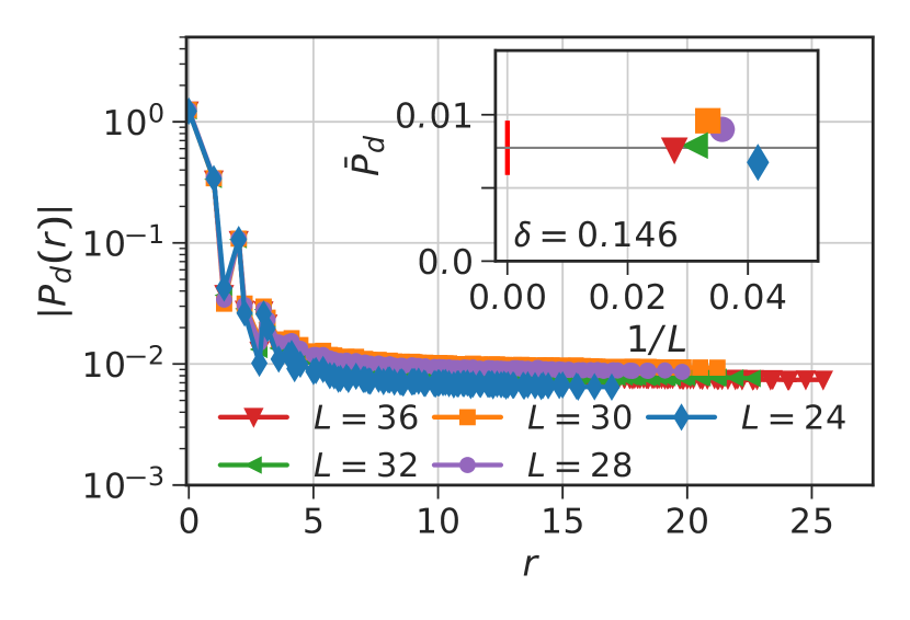
Figure 4: SC correlation function $P_{d}(r)$ for Hg1201 at $\delta=0.146$  which is close to the experimental optimal doping, at the square lattice size $L=24,28,30,32$ and $36$. Error bars are smaller than the symbol size. Inset: Size extrapolation of $P_{d}$ to the thermodynamic limit $L\rightarrow\infty$. Because of relatively scattered data we employ the average of the two biggest lattice sizes ($L=32,36$) for the size extrapolation $L\rightarrow\infty$. In fact, the value at the largest sizes is consistent with the systematic $\delta$ dependence observed near $\delta=0.146$ after the size extrapolation (not shown). The error bar at $1/L=0$ is estimated as the biggest difference to $F_{\rm SC}^{\infty}$ from the given data.

Table 3: Comparison of long-ranged SC correlation $\bar{P}_{d}^{\infty}$ and the order parameter $F_{\mathrm{SC}}^{\infty}$ with $U/|t_{1}|$ as well as comparison between $|t_{1}|F_{\mathrm{SC}}^{\infty}$ and $T_{c}^{\rm opt}$ for doped CaCuO₂ at $\delta=0.125$, and Hg1201 at $\delta=0.146$ (these values of $\delta$ are chosen in accordance with those closest to experimental optimal values, $\delta\sim 0.12$ and 0.15, respectively, and to allow the numerical size extrapolation easier). Note that the ratio $T_{c}^{\rm opt}/(|t_{1}|F_{\mathrm{SC}}^{\infty})$ is given as a nondimensional quantity by using 1 eV $=1.16\times 10^{4}$ K. The parentheses in the last digit indicate the error bar.

	$U/|t_{1}|$	$\bar{P}_{d}^{\infty}$	$F_{\mathrm{SC}}^{\infty}$	$|t_{1}|F_{\mathrm{SC}}^{\infty}$(eV)	$T_{c}^{\rm opt}$ (K)	$T_{c}^{\rm opt}/(|t_{1}|F_{\mathrm{SC}}^{\infty})$
CaCuO2	$8.10$	$0.0136(9)$	$0.116(4)$	$0.060(2)$	$110$	$0.16(1)$
Hg1201	$7.35$	$0.008(2)$	$0.09(1)$	$0.048(5)$	$90$	$0.16(2)$

III.3 Doped Bi2201 and Bi2212

In this subsection, we discuss ab initio results for Bi2212 and Bi2201 and compare them each other. Unfortunately, in these two compounds, an uncertainty exists in the experimental crystal parameters that causes the uncertainty in the effective Hamiltonian parameters as well. Especially, the distance $d^{z}_{\rm Oap}$ between an apical oxygen and the nearest Cu atom is not fully precisely determined and the available experimental data have considerable variations [48, 49, 50, 51, 52, 53]. This uncertainty is also related to the structural distortion and long-period modulation of the CuO₂ plane arising from the effect from the BiO layer [54, 55] as we discuss in Sec. V. Recent ab initio studies have clarified that this uncertainty leads to a possible variety of effective Hamiltonian parameters, especially owing to the variation of the apical oxygen position [12].

In principle, the structural optimization in ab initio calculations is desired to predict the stable atomic position. However, such an optimization in strongly correlated electron systems is at the moment not necessarily accurate enough and we leave this task for future studies. Instead, in this paper, we admit a range of Hamiltonian parameters and discuss the consequence.

As analyzed in Ref. [12], the apical oxygen position sensitively affects the effective Hamiltonian parameters, primarily the value of $U$. For Bi2212, the value $U\sim 4.2$ eV in Table 1 is intermediate and the uncertainty range is between 4.0 and 4.7 eV for $U$ by considering that $d^{z}_{\rm Oap}$ may range from 2.25 Å to 2.45 Å. On the other hand, the value $U\sim 4.4$ eV for Bi2201 in Table 1 is the upper bound and the uncertainty ranges from $U\sim 4.4$ to 3.5 eV by considering that $d^{z}_{\rm Oap}$ may range from $d^{z}_{\rm Oap}=$ 2.6 to 2.45 Å. We first present in Secs. III.3.1 and III.3.2 the results obtained from the parameters shown in Table 1, namely $U=4.2$ eV for Bi2212 and $U=4.4$ eV for Bi2201 and then discuss in Sec. III.3.3 the possible range of SC properties originating from this uncertainty later.

III.3.1 Bi2212

We begin with the results for Bi2212. Figure 5 shows $P_{d}(r)$ and $\bar{P}_{d}(L)$ at $\delta=0.167$ for $L$ from $16$ to $36$ by switching off the interlayer transfers and interactions. Namely we first show the results obtained by solving the single-layer Hamiltonian despite the actual two-layer unit cell of Bi2212. The case of $\delta$ dependent Hamiltonian is also shown in Appendix C, where the difference is small. Similarly to CaCuO₂, we identify a SC ground state with large $\bar{P}_{d}$ and it does not change significantly by increasing $L$, where the size extrapolation gives $\bar{P}_{d}^{\infty}\sim 0.0151$ as shown in the inset of Fig. 5, which corresponds to a SC order parameter $F_{\mathrm{SC}}^{\infty}\sim 0.12$. This relatively strong value of $F_{\mathrm{SC}}^{\infty}$ is understandable, because the $U/|t_{1}|$ ratio has a value of $U/|t_{1}|\sim 9.4$, which is the strongest among all four considered compounds. Again the enhanced $F_{\mathrm{SC}}^{\infty}$ originates from the larger $U/|t_{1}|$ in accordance with the observation in the comparison of Hg1201 and CaCuO₂ in Sec. III.2. This large $F_{\mathrm{SC}}^{\infty}$ is also consistent with the high $T_{c}$ (up to $\sim 100$ K) [30]. We will discuss more intricate aspect in Sec. V.

Figure 5: SC correlation function $P_{d}(r)$ for Bi2212 at $\delta=0.167$ for the square lattice size $L=16,24,30,36$. Inset: Size extrapolation of $\bar{P}_{d}$ to the thermodynamic limit. The gray line shows the linear extrapolation to $1/L\rightarrow 0$ by using the values for $L=16,24,30,36$. Error bars are smaller than the symbol size.

The competition with other phases is seen in $\delta$ dependence of the total energy shown in Fig.19 in Appendix I. Similarly to CaCuO₂, the SC state is the ground state in most of the doping concentration, while it is severely competing with spin and charge ordered states.

Now, we extend the calculation by switching on the interlayer terms and solve the two-layer Hamiltonian obtained in Ref. [12] to examine the effects of interlayer coupling. For the calculations we take two identical layers (in terms of intralayer parameters for $t_{ij}$, $V_{i}$, and $U$ where $i$ and $j$ are intralayer combination), coupled by the interlayer terms listed in Table 6 (Appendix H). The interlayer contributions are restricted to the leading interlayer hopping term of size $t_{0}^{l}=-0.098$ eV and nearest- and next-nearest-neighbor interlayer interaction of size $V_{0}^{l}=0.643$ eV and $V_{1}^{l}=0.463$ eV. See Ref. [12] for more details. A comparison between the single- and two-layer cases of $P_{d}(r)$ for $L=16$ and $\delta=0.167$ is shown in Fig. 6. We see that the long-range average of $P_{d}(\bm{r})$ in the two-layer case is close to that of $P_{d}(\bm{r})$ in the single layer case, which demonstrates that $P_{d}(\bm{r})$ is not significantly affected by the interlayer Coulomb interaction and hopping parameters. Indeed, for the single layer we found a long-range average of the SC correlation function of $\bar{P}_{d}^{\text{single}}=0.0225$, while for the two-layer compound the average is $\bar{P}_{d}^{\text{two}}=0.0213$. The corresponding values of the SC order parameter are $F_{\mathrm{SC}}^{\text{single},\infty}=0.150$ and $F_{\mathrm{SC}}^{\text{two},\infty}=0.146$, which differ by only $\sim 2.8\%$. The essentially same behavior between the single- and two-layer cases may not depend on the system size in accordance with the result of a two-layer Hubbard model at the optimum doping [56]. This similarity may be attributed to (i) the relatively small leading interlayer hopping parameter of $t_{0}^{l}=-0.098$ eV and also (ii) the robustness of the SC solution against the interlayer Coulomb interaction parameter, because the pairing occurs essentially only within a layer.

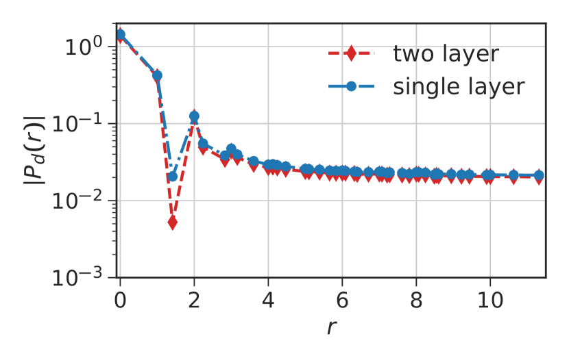
Figure 6: SC correlation function $P_{d}(r)$ for Bi2212 at $\delta=0.167$  in the cases of the single- and the explicit two-layer calculations. In the single-layer case a $16\times 16$ square lattice was considered, which corresponds to a $16\times 16\times 2$ lattice in the two-layer case. Error bars are smaller than the symbol size.

III.3.2 Bi2201

In the case of Bi2201, we again solve the single-layer Hamiltonian. The competition with other phases are seen in $\delta$ dependence of the total energy shown in Fig.20 in Appendix I.

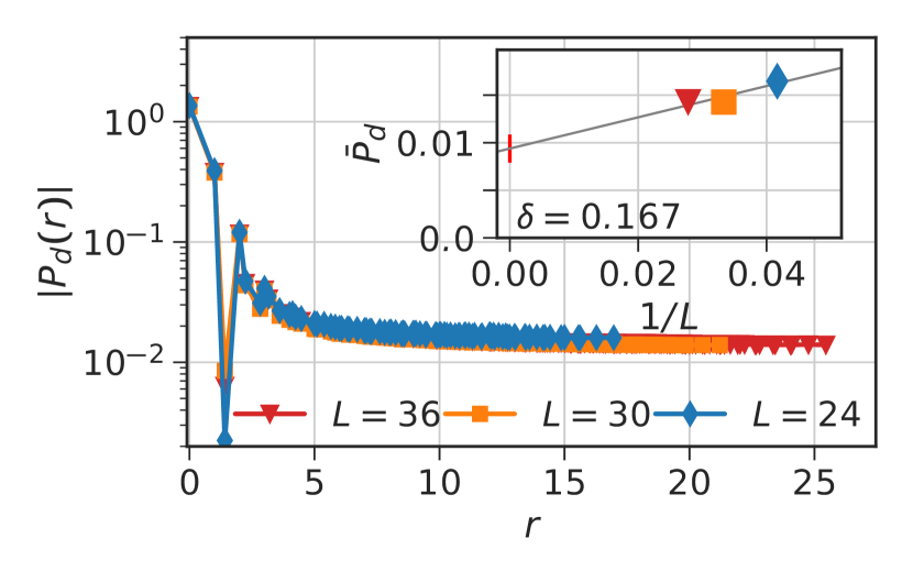
Figure 7: SC correlation function $P_{d}(r)$ for Bi2201 at $\delta=0.167$  at the square lattice sizes $L=24,30,36$. Inset: Size extrapolation of $\bar{P}_{d}$ to the thermodynamic limit. The gray line shows the linear extrapolation to $1/L\rightarrow 0$ by using the values for $L=24,30,36$. Error bars are smaller than the symbol size.

Figure 7 shows $P_{d}(r)$ and its extrapolation to the thermodynamic limit, which suggests the stable long-ranged SC order. Again, the obtained value $F_{\rm SC}^{\infty}\sim 0.10$ is consistent with the rule that larger $U/|t_{1}|$ leads to larger $F_{\rm SC}^{\infty}$ because $U/|t_{1}|$ is the second largest among the four materials in the estimate shown in Table 1. The smaller $U/|t_{1}|$ relative to Bi2212 leads to weaker SC. However, on a more quantitative aspect, we need to be careful about the uncertainty of the Hamiltonian parameter. We will discuss this issue below.

III.3.3 Effect of structural uncertainty on possible variation of SC properties

Since we have the uncertainty of the Hamiltonian parameters particularly for the interaction as we discussed above, we here monitor the effects of modifying the effective interactions for Bi2212 and Bi2201, which well represent the effect of variant apical oxygen position as shown in Appendix C of Ref. [12]. Namely, Table 1 with preserved transfer parameters fixed at each ab initio value, together with interaction scaling represents most of the effect of the apical oxygen shift and we scale the Hamiltonian (1) such that

$$\mathcal{H}(\alpha,\xi) =H_{\mathrm{kin}}+\alpha H_{U}+\xi H_{V},$$ (10)

where $\alpha=\xi=1$ represents the ab initio case given in Table 1, $\alpha$ scales the on-site Coulomb interaction term $H_{U}$, and $\xi$ scales the remaining off-site interactions $V_{i}$. Since the apical oxygen shift alters the interaction parameters in the way $\alpha\sim\xi$ [12], we examine the dependence on $\alpha=\xi$ below.

Figures 8 (a) and (b) show the size scaling and $\alpha=\xi$ dependence of $P_{d}^{\infty}$ for Bi2212 and Bi2201 at $\delta=0.167$, which is close to the experimental optimum doping. Further details are given in Sec.S5 of SM [33]. Figure 8 (c) shows the corresponding $\alpha=\xi$ dependence of the SC order parameter $F_{\rm SC}^{\infty}$. For Bi2212, by taking the realistic uncertainty range $4.0$ eV $\leq U\leq 4.7$ eV (corresponding to $0.95\leq\alpha=\xi\leq 1.1$) obtained from $2.25\,\text{\AA}$  $\leq d_{\rm Oap}^{z}\leq 2.45\,\text{\AA}$, we find the range of $0.011\lesssim P_{d}^{\infty}\lesssim 0.015$, namely $0.10\lesssim F_{\rm SC}^{\infty}\lesssim 0.12$. On the other hand, the uncertainty for Bi2201 obtained from $2.45\,\text{\AA}$ $\leq d_{\rm Oap}^{z}\leq 2.6\,\text{\AA}$ leads to $3.5$ eV $\leq U\leq 4.4$ eV (corresponding to $0.8\leq\alpha=\xi\leq 1.0$), which results in $0.00017\lesssim P_{d}^{\infty}\lesssim 0.0094$ ($0.013\lesssim F_{\rm SC}^{\infty}\lesssim 0.10$). The lower bound for Bi2201 causes a fatal damage to the SC order.

Figure 8: Variation of SC order arising from uncertainty of the apical oxygen position via $\alpha=\xi$ scaling for Bi2212 and Bi2212. The realistic range is $0.95\leq\alpha=\xi\leq 1.1$ for Bi2212 and $0.8\leq\alpha=\xi\leq 1.0$ for Bi2201. Size extrapolation of $\bar{P}_{d}$ for: (a) Bi2212 at $\delta=0.167$ and $\alpha\in\{0.8,0.9,1.0,1.1,1.2\}$, (b) Bi2201 at $\delta=0.167$ and $\alpha\in\{0.8,0.9,1.0\}$. (c) $F^{\infty}_{\mathrm{SC}}$ as a function of $\alpha=\xi$ for Bi2212 (orange) and Bi2201 (blue).

Table 4 summarizes the size-extrapolated $\bar{P}_{d}^{\infty}$ and corresponding $F_{\mathrm{SC}}^{\infty}$ for the two Bi compounds when we use the Hamiltonian parameters listed in Table 1 and when we admit the uncertainty range of the interaction parameters for Bi2212 and Bi2201. The scaling Eq.(9) proposed for CaCuO₂ and Hg1201 is also valid in the Bi compounds and the experimental $T_{c}^{\rm opt}$ is within the inferred range. We conclude that its materials dependence is well captured for the four studied materials (see also Fig. 11 in Sec. VI).

Table 4: Comparison of long-ranged SC correlation $\bar{P}_{d}^{\infty}$ and the order parameter $F_{\mathrm{SC}}^{\infty}$ with $U/|t_{1}|$ for Bi2212 and Bi2201 at $\delta=0.167$, which is chosen in accordance with the experimental optimal values. The range of values represents the uncertainty range arising from the uncertainty of the apical oxygen position. This estimate helps the inference of the correct apical oxygen position (see text).

	$U$	$U/|t_{1}|$	$\bar{P}_{d}^{\infty}$	$F_{\mathrm{SC}}^{\infty}$	$0.16|t_{1}|F_{\mathrm{SC}}^{\infty}$ (K)	$T_{c}^{\rm opt}$ (K)
Bi2212	4.0-4.7	8.8-10.4	$0.011$ - $0.015$	$0.10$ - $0.12$	83-101	85-100
Bi2201	3.5-4.4	6.7-8.4	$0.00017$ - $0.0094$	$0.013$ - $0.096$	12-93	10-40

We realize that the fragility and diversity of $T_{c}^{\rm opt}$ experimentally observed in the range $10<T_{c}^{\rm opt}<40$ K for Bi2201 is accounted for by the range of actual apical oxygen position. This range may be caused by the type of dopant atoms, impurities, and the spatial inhomogeneity caused by the supermodulation, which may depend on samples and the amplitude of the modulation. In fact, it was observed that the $d_{\rm Oap}^{z}$ periodically varies as much as 6% in accordance with the supermodulation for Bi2212 and a comparable modulation may exist for Bi2201 as well, which can be the origin of the experimental uncertainty [54, 55]. The basic origin of this diversity and relatively low $T_{c}$ among the four families of compounds is attributed to relatively small $U/|t_{1}|$ in the lower uncertainty range, at which the SC order becomes sensitively damaged by a slight decrease of $U/|t_{1}|$. We discuss more general aspects of the interaction dependence in Sec. IV. Even when we admit the uncertainty range, the general trend about the weaker SC of Bi2201 than those of Bi2212 is well explained by this ab initio result. It can also safely be addressed that Bi2212 has one of the strongest SC and $T_{c}^{\rm opt}$ among the four families comparably to CaCuO₂.

The effects of apical oxygen position on Hamiltonian parameters are discussed in Sec. V and in Appendix L.

IV Results beyond ab initio: interaction dependence of superconducting order

We now study SC properties beyond the ab initio results. Ab initio results in the previous section successfully reproduce the experimental trend and have revealed that $U/|t_{1}|$ is the principally important Hamiltonian parameter to control the SC order parameter. Therefore, it is intriguing to examine the optimum Hamiltonian parameters to maximize the order parameter and hence the optimum $T_{c}$ beyond the existing materials for the purpose of materials design to seek for higher $T_{c}$ superconductors. We present $U/\lvert t_{1}\rvert$ dependence of $F_{\rm SC}$ as well as dependence on off-site interaction when tuning the interaction parameters artificially away from the ab initio value while keeping transfer parameters fixed at ab initio values. We here take an example of CaCuO₂ Hamiltonian at $\delta=0.167$ and monitor the effect of $\alpha$ and $\xi$ dependencies defined in Eq. (10).

We examine three types of scaling to go beyond the ab initio Hamiltonian: (i) Scale only the on-site Coulomb interaction by $\alpha$ with fixed $\xi=1.0$ ($\mathcal{H}(\alpha,1.0)$), (ii) Scale the full interaction part equally by using $\alpha=\xi$ (namely, $\mathcal{H}(\alpha,\alpha)$), and (iii) Fix $\alpha=1.2$ and scale the off-site Coulomb interaction uniformly via $\xi$ by employing $\mathcal{H}(1.2,\xi)$, by considering the fact that (ii) shows the maximum SC order at $\alpha=\xi=1.2$. For the cases (i) and (ii) we chose scaling values $\alpha$ ranging from $0.6$ up to $4.0$ while for the third case the range from $0.0$ to $2.0$ is chosen. Since the size dependence is not appreciable, we study $L=24$ lattice. The SC order parameter $F_{\rm SC}$ are shown in Fig. 9 (a) at $\delta=0.167$ hole doping.

The results show that the SC order parameter can be enhanced with the amount of around 30% from the ab initio value when the interaction parameter is tuned to $\alpha\sim 1.2$ for (i) and around 20% at $\alpha=\xi\sim 1.2$ for (ii), which may allow $T_{c}^{\rm opt}$ as much as $\sim 130\text{--}140\,\text{K}$, when compared to the ab initio results for CaCuO₂.

In the tuning (iii), we find that the order parameter further increases up to $F_{\rm SC}^{\infty}\sim 0.22$ by decreasing $\xi$, which is twice as large as the ab initio case. However, we keep in mind that on-site and off-site interactions cannot independently be controlled in the usual experimental conditions. The present result offers a guide to enhance the SC in designing artificial structure and metamaterials including surface and interface, where quicker screening of the off-site interaction is desirable by keeping the on-site interaction at the optimal value (in this case $\alpha=1.2$).

Another limitation to be considered is the competition with the stripe and AFM order. As far as we restrict the on-site interaction within the ab initio range, the SC energy is always lower than that of the stripe state as one sees in Fig. 9 (b). Here, we show the competition with the C4S8 because it is established that the most severe competitor is the C4S8 state. However, the decreasing of energy difference, such as at ($\alpha=1.2$, $\xi=0$), where the difference is $\leq 2\,\text{meV}$, may result in the thermal destruction of the SC order. For $\xi\geq 0.2$ the SC is still a stable ground state, while at small $\xi$, $F_{\rm SC}$ becomes nearly twice of the ab initio value for the doped CaCuO₂.

Figure 9: (a) $F_{\rm SC}$ over scaling $\alpha$ or $\xi$ (effective scaling of $U/\lvert t_{1}\rvert$ and $V_{i}/U$) of the SC state on the $L=24$ square lattice and $\delta=0.167$ hole doping. The inset is an enlarged plot around the peak $0.9<\alpha,\xi<1.5$. For further details see the main text. (b) Variance extrapolated energy difference $\Delta E$ between the SC and C4S8 as a function of $\xi$ in the case $\mathcal{H}(\alpha=1.2,\xi)$.

The order parameter decreases when $U/|t_{1}|$ is too large beyond the realistic range of the cuprates studied in this paper as we see in Fig. 9 (a). This reduction was already pointed out on the level of the Hubbard model [9]. The reduction at large $U/|t_{1}|$ is studied in Appendix J, which shows nontrivial power-law dependence of $F_{\rm SC}$ on $U/|t_{1}|$. The reduction itself may be easily understood on a qualitative level from the suppression of charge fluctuation with increasing $U/|t_{1}|$, which also suppresses the quantum entanglement caused by the suppression of both spin singlet fluctuation and dynamical exciton generation as was reported in the literature [9, 57]. It was pointed out that the enhanced quantum entanglement can be achieved by the fractionalization of electrons [57, 58], which may be maximized at the optimum $U/|t_{1}|$.

V Discussion

By assuming the same ratio $T_{c}/(|t_{1}|F_{\rm SC}^{\infty})\sim 0.16$ with CaCuO₂ and Hg1201, we can infer the range of $T_{c}$ arising from the uncertainty of the apical oxygen position and resultant uncertainty of $U/|t_{1}|$ listed in Table 4. The range of inferred $T_{c}$ listed in Table 4 for Bi2212 is consistent with the experimentally observed range of $T_{c}^{\rm opt}$ within the error bars. This suggests that the sample dependence of $T_{c}^{\rm opt}$ may be accounted for by the sample dependence of the apical oxygen position.

We note that the order parameter $F_{\rm SC}^{\infty}\sim 0.10$ obtained here for Bi2212 and Bi2201 also shows consistency with the result obtained by using the machine learning of the angle-resolved photoemission spectroscopy data for Bi2212 and Bi2201, respectively, at the optimum doping [59], which gave $\langle c_{k\uparrow}c_{-k\downarrow}\rangle\sim 0.065$ at the antinodal point for Bi2212 and the momentum averaged value $\sim 0.063$ for Bi2201 at the optimum doping. These are translated commonly to $F_{\rm SC}^{\infty}\sim 0.09$ in the present definition of $F_{\rm SC}^{\infty}$ because of the relation $F_{\rm SC}^{\infty}=\sqrt{2}\langle c_{k\uparrow}c_{-k\downarrow}\rangle$.

In the case of Bi2201, the estimated $0.16|t_{1}|F_{\rm SC}^{\infty}$ is also listed in Table 4. The comparison with the sample dependence of experimental $T_{c}$ suggests that the true apical oxygen position is distributed near the lower bound $d^{z}_{\rm Oap}\sim 2.45$Å, if it is spatially uniform. Alternatively if the supermodulation exists, the lower bound of $d^{z}_{\rm Oap}$ in the modulation may be close to 2.45 Å, because it governs the SC order as the bottleneck. It is desired to test this inference by precise and simultaneous measurements of the relation between $T_{c}$ and $d_{\rm Oap}^{z}$ for Bi2212 and Bi2201.

The order parameter $F_{\rm SC}^{\infty}$ increases with decreasing hole doping for $\delta>0.05$ as we find in Fig. 2, which follows the same trend as the SC gap as we discussed, but is slightly different from the dome structure known for $T_{c}$ in the cuprates, where the peak of the dome is located at higher $\delta$. Complete and quantitative understanding of this different trend is not the scope of this paper and is left for future studies. However, the origin of this difference can be inferred to be attributed to the increasing damping and incoherence of electrons in the underdoped region toward the metal-insulator transition as was analyzed before [44, 45], which is represented as the enhanced self-energy of the normal electrons toward the Mott insulator. In the experimental conditions, the atomic doping/substitution introduces atomically spatial inhomogeneity, which is ignored in the present study and may cause the localization of carriers, which could also be the origin of slower increase of $T_{c}$ upon doping.

In Appendix K, we show a qualitative difference of the momentum distribution between the optimal and underdoped hole concentrations, which suggests a signature of the increased damping at lower carrier concentration within the present ab initio study. We also discuss in Appendix K the subtlety and complexity in the underdoped region due to the pseudogap formation, involved in several quantities, which is not the scope of this paper.

The $\delta$ dependence of the energy decomposed to the kinetic, on-site and off-site interaction energies are analyzed in Appendix G. It should be noted that the on-site interaction energy $E_{U}=\langle\mathcal{H}_{U}\rangle$ has a convex curvature as a function of $\delta$, which contributes to the effective attraction of electrons despite the original strong repulsion $U$. In fact, the $U/|t_{1}|$ dependence of the local attraction is qualitatively consistent with $F_{\rm SC}$ in Fig. 9. See Appendix G for more details. The local effective attraction may cause the Cooper pairing as well as the stripe formation. It was pointed out that the convex curve of the local energy generates bistable excitations, one in the underdoped side and the other in the overdoped side, inducing the electron fractionalization and the enhanced quantum entanglement through the quantum tunneling of the two excitations [57, 58]. This line of further research is an important future subject.

The importance of the apical oxygen position has been pointed out from various viewpoints [60, 61, 62, 63]. In this paper, we have elucidated the crucial role of controlling $U$ in general in the single-band description, which quantitatively explains the variation of $T_{c}^{\rm opt}$ and its uncertainty in the Bi compounds. In addition, the modulation of the SC gap with the modulation of the apical oxygen position in Bi2212 has indicated that the longer $d_{\rm Oap}^{z}$ induces the smaller SC gap [55]. This is consistent with the trend of $F_{\rm SC}^{\infty}$, which decreases when $\alpha$ is increased in the realistic range as shown in Fig. 8. This indicates that Bi2212 is located already slightly above the peak in the $\alpha$ dependence of $F_{\rm SC}^{\infty}$, which corresponds to $\alpha=1.2$ for doped CaCuO₂ shown in Fig. 9. The present observation is also in accordance with the effect observed by laser irradiation aiming at the displacement of the apical oxygen position [64]. The control of $d_{\rm Oap}^{z}$ if possible in a spatially uniform fashion may help to optimize the SC in which the disturbance and pair breaking by the randomness caused by the inhomogeneous supermodulation in the case of the Bi compounds could be avoided.

The effects of the displacement of the apical oxygen position on the Hamiltonian parameters were discussed in Ref. [12]. In Appendix L, we readdress this issue in relation to earlier work.

We have mainly focused on the quantities at optimal doping to clearly extract the diversity of the materials dependence, where the experimental subtlety due to the effects from extrinsic randomness as well as the complexity of physical quantities arising from the pseudogap formation in the underdoped region is irrelevant. The behavior of suppressed $T_{c}$, the SC carrier density $n_{s}$, and the coherent spectral weight arising from the pseudogap formation in the underdoped region are left for future studies. See Appendix K for more details.

In general, the $d$-wave SC correlation has a dip at (1,1) distance. The origin is speculated as follows: The singlet pair between electrons at (0,0) and (1,0) sites dynamically interfere with the singlet pair between (1,1) and (1,0), because these two singlets are incompatible. The same is true for the singlets, which share (0,1) site. This double interfere makes the SC correlation of the pair between (0,0) and (1,1) smaller very generally. However, at the moment, we do not know the origin of particularly large dip around $\delta=1/8$, which is left for future study.

There exist studies proposing the possibility of the pair-density-wave (PDW) states [65]. However, in the present ab initio Hamiltonians, the PDW correlation remains small as is shown in Fig. S7 of SM [33], where peak is absent at nonzero momentum. If the stripe long-ranged order coexists in the SC ground state, the PDW order must be trivially accompanied. However, as one sees in Figs. 14(b) and S6, the stripe correlation exists but remains small and is scaled to zero in the thermodynamic limit.

In this paper, we have employed the single-band Hamiltonian for the AB orbital, because the hybridization gap between AB and B or NB orbitals is so large ($\sim 8-9$ eV) that the B and NB bands are more or less completely filled and inactive (see Fig. 10(b) of Ref. [34] and Appendix D of Ref. [12]). When one starts from the three bands constructed from Cu 3$d_{x^{2}-y^{2}}$ and O 2$p_{\sigma}$ atomic orbitals, the analysis would be more complicated. See Appendix M for this issue.

VI Summary and conclusions

We have studied the superconductivity in the ab initio Hamiltonians for CaCuO₂, Hg1201, Bi2201, and Bi2212 derived by using the experimental crystal structure in Ref. [12] without adjustable parameters . The dominance of SC order against severely competing stripe states and AFM state in a wide range of hole concentration is shown in the solutions for the ground state of all four materials obtained from the variational Monte Carlo calculations, which agrees with the experimental results.

The SC order parameter $F_{\rm SC}^{\infty}$ at the optimal doping shows consistency with the superfluid density measured in the $\mu$SR and the machine learning analysis of the ARPES data for Bi2212 and Bi2201. $F_{\rm SC}^{\infty}$ decreases with increasing doping for the doping concentration $\delta>0.05$, showing a similarity to the SC gap reported in the STM and ARPES measurements. On the other hand, $F_{\rm SC}^{\infty}$ quickly decreases to zero toward $\delta=0$ for $\delta<0.05$ forming a dome structure which has a similarity to experimental $T_{c}$, but the dome peak appears at slightly lower $\delta$ for the calculated $F_{\rm SC}^{\infty}$. This may be attributed to the reduced renormalization factor suggested by the broadened momentum distribution.

From the comparison of the four materials, we have revealed that $U/|t_{1}|$ is a crucial parameter to control the strength of the SC order; larger $U/|t_{1}|$ materials show larger SC order parameter $F_{\rm{SC}}^{\infty}$ in the realistic materials. This explains that $T_{c}$ and the SC gap at the optimum doping are larger for CaCuO₂ than Hg1201, where $T_{c}^{\rm opt}$ is well scaled by $\lvert t_{1}\rvert F_{\rm SC}^{\infty}$ as $T_{c}^{\rm opt}\sim 0.16\lvert t_{1}\rvert F_{\rm{SC}}^{\infty}$. Though the experimental uncertainty in the crystal structure prohibits a quantitative comparison, $F_{\rm SC}^{\infty}$ is also larger for Bi2212 than Bi2201 at least qualitatively, in agreement with the experimental indications. When we apply the same scaling $T_{c}^{\rm opt}\sim 0.16\lvert t_{1}\rvert F_{\rm SC}^{\infty}$ to the two Bi compounds with the calculated order parameter, it also well explains the experimental sample dependence of $T_{c}$. The strong dependence of $F_{\rm SC}^{\infty}$ on $U/|t_{1}|$ for real materials are summarized in Fig. 10: In the range of $7.0\leq U/|t_{1}|\leq 8.0$, $F_{\rm SC}^{\infty}$ sharply increases and the calculated sensitive materials dependence of $F_{\rm SC}^{\infty}$ is well captured within this range. This simply means that, except for Bi2212, most of the realistic materials we have studied are positioned in the weak-coupling side, where the SC order parameter rapidly increases with increasing $U/|t_{1}|$. The good scaling of $T_{c}^{\rm opt}$ by $0.16|t_{1}|F_{\rm{SC}}^{\infty}$ is also summarized in Fig. 11, which indicates that the detailed difference of $U/|t_{1}|$ within the range of $7<U/|t_{1}|<9$ in the ab initio parameters reproduces the diverse materials dependence of $T_{c}^{\rm opt}$. Since the larger variance for the theoretical prediction on Bi2201 is ascribed to the experimental uncertainty of the apical oxygen, it is desired to precisely determine the apical oxygen position in the experiments.

Figure 10: $F_{\rm{SC}}^{\infty}$ as a function of $U/|t_{1}|$ for the four cuprate compounds at $\delta=0.167$ plotted from the list in Tables 3 and 4.

Figure 11: Experimental $T_{c}^{\rm{opt}}$ (black crosses or bars) in comparison to the $T_{c}=0.16\lvert t_{1}\rvert F_{\rm{SC}}^{\infty}$ scaling for each compound (purple bars). $T_{c}$ is taken from Tables 3 and 4.

Based on the successful reproduction of the materials dependent properties, the underlying superconducting mechanism is identified by the effective local attraction emerging from the Mottness, which converts the original strong repulsion to the attraction.

The SC order parameter has the maximum above the ab initio values of $U/|t_{1}|$ at 20% larger value of $U/|t_{1}|$ with the enhancement of 20%-30%. If one can control on-site and off-site interaction independently, further optimization of the SC order parameter as much as the factor 2 larger value beyond the available compounds synthesized so far without falling into other competing states can be achieved as the theoretical maximum value in the present mechanism. By increasing $|t_{1}|$ as well as the whole parameter values uniformly, $T_{c}^{\rm opt}$ should obviously increase accordingly. These offer a clue for the materials design in the future.

Appendix A Lanczos method and restricted Boltzmann machine procedure

Lanczos method

To further improve the accuracy of the VMC calculations or the variance extrapolation of the competing ground state candidates, we apply the Lanczos method [42]. To do so the optimized mVMC wave function $\ket{\Psi}$ is extended by

$$\ket{\psi_{n}}=\left(1+\sum_{n=1}^{M}\alpha_{n}\mathcal{H}^{n}\right)\ket{\Psi}.$$ (11)

The factor in front of $\ket{\Psi}$ can be regarded as an additional projection operator with variational parameters $\alpha_{n}$, which–when chosen appropriately–further reduce the energy. Although one could systematically improve the wave function by increasing $M$, the computational cost increases exponentially with $M$, too. Hence we employ the Lanczos method only up to the first step ($n=1$) within this work.

Restricted Boltzmann machine procedure

To further improve the mVMC wave function we apply a restricted Boltzmann machine as a variational wave function $\ket{\Psi}$, as first suggested in Ref. [66]. Here we follow the notations given in Refs. [20, 42]. The variational wave function including RBM takes the following form

$$\ket{\Phi}=\mathcal{P}^{\mathrm{G}}\mathcal{P}^{\mathrm{J}}\mathcal{P}^{\mathrm{dh}}\mathcal{N}\ket{\phi^{\mathrm{pair}}},$$ (12)

where $\mathcal{N}$ is the additional RBM correlator. The RBM correlator

$$\mathcal{N} =\prod_{k}2\cosh\left(b_{k}+\sum_{i}W_{ik}\sigma_{i}\right)\mathrm{e}^{\sum_{i}a_{i}\sigma_{i}}$$ (13)

introduces the additional variational parameters $b_{k}$ (hidden layer), $a_{i}$ (visible layer), and $W_{ik}$ (network).

In practice we apply the additional RBM projection after the wave function was already optimized via mVMC calculations, i.e., the variational parameters of the optimized wavefuction $\ket{\phi}=\mathcal{P}^{\mathrm{G}}\mathcal{P}^{\mathrm{J}}\mathcal{P}^{\mathrm{dh}}\ket{\phi^{\mathrm{pair}}}$ are kept fixed during the RBM procedure.

The accuracy of the wave function depends on the number of hidden and visible parameters ($N_{h}$, $N_{v}$) [66]. Hence we can define a hidden variable density as $\alpha_{\rm RBM}=N_{h}/N_{v}$ as measure for the accuracy. Note that the number of RBM variational parameters increases with $\alpha$, too.

Within this work the RBM procedure was applied with $\alpha_{\rm RBM}=4$.

Appendix B Variance Extrapolation Procedure

The total energy per site $E/N=\braket{\mathcal{H}}/N$ is calculated after the variance extrapolation. The true ground state as a function of the variance $(\delta E)^{2}=(\braket{\mathcal{H}^{2}}-\braket{\mathcal{H}}^{2})/\braket{\mathcal{H}}^{2}$ is obtained by taking the limit $\delta E\rightarrow 0$, because the true eigenstate satisfies $\delta E=0$ [39, 40, 41]. If several different states such as SC, spin- and charge-ordered as well as normal metallic states are competing, the ground state is determined from the lowest-energy state after the variance extrapolation. In practice, the variance extrapolation is a linear regression of the energies per site $E/N$ (e.g. obtained from combinations of mVMC, Lanczos, or RBM) over the variance $\delta E$ for a specific state, to approximate the zero variance value of the energy.

Figure 12: Variance extrapolation for the example of CaCuO₂ at $\delta=0.167$ on a $L=24$ lattice. The inset shows an enlarged plot around $(\delta E)^{2}=0$.

As an example the variance extrapolation for $\delta=0.167$ in CaCuO₂ is shown in Fig. 12. From the inset we confirm the lowest energy of the SC state with severely competing AFM and stripe states very close to it (the difference is around $5\,\text{meV}$). However, the overlap of the error bars is small and in comparison to AFM, C4S8 and C3S3 states, the SC state definitely has lower energy.

Appendix C Results of $\delta$ Dependent Hamiltonian

The hole density dependence of $F_{\rm SC}$ at $L=24$ is compared between the case presented in the main text and that calculated by the $\delta$ dependent Hamiltonian given in Sec. S1B of SM [33]. The results for CaCuO₂ in Fig. 13(a) and for Bi2212 in Fig. 13(b) show that the difference of the two Hamiltonians is small and essential feature can be analyzed by taking the Hamiltonians analyzed in the main text.

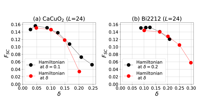
Figure 13: Comparison of $F_{\rm SC}$ between that obtained by using $\delta$ dependent Hamiltonians (red) and the fixed Hamiltonian (black) as in the main text.

Appendix D Thermodynamic limit of the trial wave function after optimization for CaCuO₂

Here we discuss the stability of the AFM, C3S3, and C4S8 states in the thermodynamic limit for CaCuO₂. To do so, each state is stabilized on different lattice sizes and the spin and charge structure factors ($S_{s}(\bm{q})$ and $S_{c}(\bm{q})$) are calculated.

We plot $S_{s}(\bm{q})$ as a function of $1/L$ or $1/L^{2}$ depending on the cases of the presence or absence, respectively, of the AFM order by following the convention and perform a linear extrapolation. The result is shown in Fig. 14, where in Fig. 14(a) the peak height of the spin structure factor follows a linear trend with a nonzero offset, indicating a stable long-ranged AFM order. In Fig. 14(b), the peak of the spin structure is scaled to zero in the thermodynamic limit, which indicates the absence of the long-ranged AFM order in the SC state at this doping. We did not find the coexistence of the SC and AFM order at other doping, either.

Figure 14: Size dependence of the spin structure factor $10^{3}\times S_{s}(\bm{q}_{\mathrm{max}})/N$ at $(\pi,\pi)$ for (a) the AFM state after optimization at half filling ($L=12,16,24$) and $\delta=0.167$ ($L=12,18,24$), and for (b) the SC state at $\delta=0.167$ for different lattice sizes ($L=24,30,36$).

The size scaling of the charge-stripe states is shown in Fig. 15. Although the plot of the size dependence is not sufficient due to very demanding computational cost for larger sizes, the trend suggests that only the C4S8 state shows a clear long-ranged order of spin and charge at around $\delta=0.125$ in the thermodynamic limit. The C3S3 state seems to collapse to a paramagnetic state at the chosen doping of $\delta=0.207$, at which C3S3 has relative stability. Hence we use the labeling “C3S3-like” instead of C3S3 in the main text. We do not go into details of the size dependence for the stripe-like states, because they are in any case excited states.

Figure 15: Size dependence of the charge and spin stripe state after the optimization of variational parameters for different lattice sizes and fillings. For C3S3 (red crosses) $\delta=0.207$ and $L=12,24$ and for C4S8 (blue dot) $\delta=0.125$ and $L=16,24$. (a) $10^{3}\times S_{s}(\bm{q}_{\mathrm{SDW}})/N$ vs $1/L$. (b) $10^{3}\times S_{c}(\bm{q}_{\mathrm{CDW}})/N$ vs. $1/L^{2}$. ${\bf q}_{\rm SDW}$ and ${\bf q}_{\rm CDW}$ are the wave numbers at the peak of $S_{s}$ and $S_{c}$, respectively, for the spin density wave (SDW) and charge density wave (CDW) modulations, respectively. The dashed lines are only to guide the eyes.

Appendix E Comparison to Hubbard model studies

Here we discuss the crucial difference of the ab initio results from the extensively studied Hubbard models without the off-site interaction. In the Hubbard model studies, irrespective of the presence of the next-nearest transfer $t_{2}$ or absence of it, in the hole doped region, a broad consensus seems to be formed, where the ground state has stripe type long-ranged charge order [3, 5, 6, 67, 68, 69, 70, 71, 72]. The charge and spin stripe states were also suggested to coexist with weak SC order in some cases [5, 72], but other studies did not find the SC order [6, 68, 69, 71].

In the Hubbard model studies, the numerical methods have a variety including the present VMC, density matrix renormalization group, constrained path quantum Monte Carlo, tensor network and density matrix embedding theory, which have their own advantages and disadvantages and they are complementary. When they can be compared with reliable solutions, the above Hubbard model calculations were benchmarked, which have shown comparable accuracy when compared between each state-of-the-art updated version. Even in quantum spin models, the level of accuracy of the above methods is roughly similar [21]. We also refer to recent thorough comparisons [73].

On the other hand, when realistic off-site interaction is included, the ground state is reported to be charge homogeneous superconducting state [10]. The off-site interaction substantially suppresses the SC order but the charge and spin stripe states are more damaged by the frustration introduced by the off-site interaction. The role of off-site interaction for the stabilization of the SC state relative to the stripe state was directly demonstrated in Ref. [10] by the comparison of ab initio result and that of the Hamiltonian obtained by switching off only the off-site interactions. We confirmed the similar behavior for the present Hamiltonians. The absence of developed stripe correlations in the SC ground state is seen in Fig. 14 herein and in Fig.S6 of SM [33].

Appendix F $t_{2}$ dependence

Figure 16: SC correlation function $P_{d}(r)$ for modified $t_{2}$ from the CaCuO₂ Hamiltonian for $L=24$ lattice.

Figure 17: SC order parameter $F_{\rm SC}$ as a function of $\delta$ calculated for three choices of $t_{2}$ modified from from CaCuO₂ Hamiltonian.

Here we show $t_{2}$ dependence of $F_{\rm SC}$ by starting from the ab initio Hamiltonian for hole doped CaCuO₂ with other Hamiltonian parameters fixed, where the effect of $t_{2}$ is monitored beyond the ab initio value primarily within the realistic range of $|t_{2}/t_{1}|$ ($0.2\leq|t_{2}/t_{1}|\leq 0.3$) in Figs. 16 and 17 for $L=24$ lattice. $F_{\rm SC}$ slightly decreases with increasing $t_{2}$, which is qualitatively consistent with a different approach [63]. However, the variation of $F_{\rm SC}$ is at most 10% near the optimum doping in the realistic range. Furthermore, $F_{\rm SC}$ has essentially no $t_{2}$ dependence in the range $0.0\leq|t_{2}/t_{1}|\leq 0.2$. On the other hand, the period of the stripe order is known to sensitively depend on $t_{2}$ [6, 5, 72, 68, 69, 71] in the ground states of Hubbard models and it may alter the superconductivity if it coexists, while the present charge uniform superconducting ground state is quite different.

Appendix G Analysis of $\delta$ dependence of energy

In Fig. 18 the total energy per site $E_{\rm tot}$ and the on-site Coulomb part $E_{U}$ (see panel (a), (c), respectively) are shown for doped CaCuO₂. Each energy contribution is subtracted by a linear function $F(\delta)=b_{0}+b_{1}\delta$ for better visibility, where $b_{0}$ and $b_{1}$ are listed in Table 5 (see gray lines in (a), (c)) and are shown in (b), (d). The subtracted energies are fitted by a quadratic function $\mathcal{P}(\delta)=c_{0}+c_{1}\delta+c_{2}\delta^{2}$ to examine the curvature. Explicit values of the parameters are given in Table 5.

The result shows that the total energy is concave as a function of $\delta$ of course, which is required from the thermodynamic stability, while only $E_{U}$ exhibits convex behavior with $c_{2}<0$. Because the effective particle interaction is given by the $\delta^{2}$ term, we find that the local quantity $E_{U}$ is the origin of the attraction while the nonlocal energies contribute to $c_{2}>0$ in the total energy ensuring the thermodynamic stability. This supports the idea that the local strong correlation (repulsion) called Mottness turns to originate the effective attraction of the electrons, which is the underlying mechanism of both of the Cooper pairing and charge segregation such as the stripes. The attraction is understood from the following Mottness: The local energy is retained high in the Mott insulator because of $U$. However, if the carrier is doped, this is released by acquiring the itinerancy in a nonlinear fashion as a function of $\delta$ which yields $c_{2}<0$ and the attraction. In accordance with the $\alpha$ dependence of $F_{\rm SC}$, $c_{2}$ shows a similar behavior as $-c_{2}=1.47,2.24,2.13,1.85$ and 1.53 at $\alpha=1.0,1.1,1.2,1.3$ and 1.4, respectively with a peak around $\alpha\sim 1.1$-1.2.

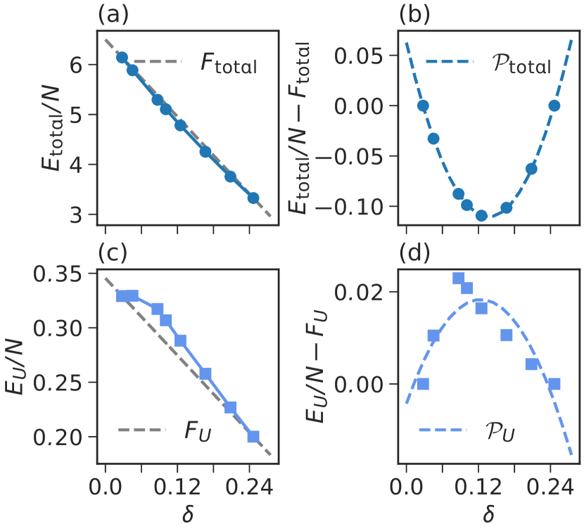
Figure 18: Energy per site as a function of $\delta$ in the SC state on a $L=24$ square lattice. Total energy $E_{\mathrm{total}}/N$ (a), and $E_{\mathrm{total}}/N-F(\delta)$ (b) as well as on-site Coulomb energy $E_{U}/N$ (c), and $E_{U}/N-F(\delta)$ (d) are plotted. Here, a $\delta$-linear function $F(\delta)$ defined below is subtracted in (b) and (d) for better visibility. Note that $F(\delta)$ is different depending on the type of the energy as seen in Table 5. The gray line in the left column indicates $F(\delta)=b_{0}+b_{1}\delta$, which is subtracted in (b) and (d). Right column: Energies after subtraction of $F(\delta)$ are fitted via a quadratic function $\mathcal{P}(\delta)=c_{0}+c_{1}\delta+c_{2}\delta^{2}$. Fitting parameters are given in Table 5.

Table 5: Fitting parameters of linear correction function and quadratic fit function discussed in Fig. 18. See the main text for the explanation.

	$b_{0}$	$b_{1}$	$c_{0}$	$c_{1}$	$c_{2}$
$E_{\mathrm{total}}/N$	$6.4995$	$-11.9723$	$0.0626$	$-2.5274$	$9.2307$
$E_{U}/N$	$0.3455$	$-0.5900$	$-0.0043$	$0.3651$	$-1.4749$

Appendix H Interlayer contributions for Bi2212

Table 6: Effective interlayer Hamiltonian parameters (in eV) for Bi2212 at $\delta=0.2$ taken from Ref. [12].

Bi2212
$V^{l}_{0}$	$V^{l}_{1}$	$V^{l}_{2}$	$V^{l}_{3}$	$V^{l}_{4}$	$V^{l}_{5}$	$V^{l}_{6}$
$0.643$	$0.463$	$0.368$	$0.291$	$0.262$	$0.220$	$0.120$
$t^{l}_{0}$	$t^{l}_{1}$	$t^{l}_{2}$	$t^{l}_{3}$	$t^{l}_{4}$	$t^{l}_{5}$	$t^{l}_{6}$
$-0.098$	$-0.001$	$0.019$	$-0.010$	$0.007$	$0.000$	$-0.003$

The effective interlayer Hamiltonian parameters for Bi2212 are shown in Table 6, where $V^{l}_{n}$ is the interlayer Coulomb interaction, and $t^{l}_{n}$ the interlayer hoppings. As defined in Ref. [12], the notation $n=0$ represents the interaction or hopping between interlayer nearest-neighbor Cu atoms (located one above the other), and $n\geq 1$ represents the interaction or hopping between a Cu atom and its $(n+1)$th interlayer nearest-neighbor (located above or below its intralayer $n$th nearest-neighbor).

Figure 19: Variance extrapolated energies of Bi2212 for various ground-state candidates (SC, charge/spin stripe C3S3 and C4S8, and AFM states) as a function of hole doping $\delta$ on a $L=24$ square lattice. (a) Total energies per site subtracted by $\mathcal{F}(\delta)$. All energies are subtracted by the function $\mathcal{F}(\delta)=-12.34985\cdot\delta+6.36953$. (b) Energy difference $\Delta E$ for the variance extrapolated data from (a).

Figure 20: Variance extrapolated energies of Bi2201 for various ground-state candidates (SC, charge-spin stripe (C3S3 and C4S8), and AFM state) as a function of hole doping $\delta$ on a $L=24$ square lattice. (a) Total energies per site subtracted by $\mathcal{F}(\delta)$. All energies are subtracted by the function $\mathcal{F}(\delta)=-15.38797\cdot\delta+7.79753$. (b) Energy difference $\Delta E$ for the variance extrapolated data from (a).

Appendix I Doping dependence of energy for Bi2201 and Bi2212

The energy per site as a function of $\delta$ and the competition of SC, stripe and AFM states is shown in Fig. 19 for Bi2212 and Fig. 20 for Bi2201.

Appendix J Scaling of the SC order in strong-coupling region

Figure 21: SC order parameter in strong-coupling region for $\delta=0.101$ and 0.167. The lattice size is $L=24$. The dashed lines are fitting $F_{\rm SC}\propto(|t_{1}|/U)^{p}$ with $p=0.58$ for $\delta=0.167$ and $p=0.60$ for $\delta=0.101$.

The SC order parameter $F_{\rm SC}$ in the strong-coupling region is plotted in Fig. 21 by monitoring $U$ with other paramters of the Hamiltonian fixed at the ab initio values of CaCuO₂ for $L=24$ lattice. $F_{\rm SC}$ is scaled as $F_{\rm SC}\sim(|t_{1}|/U)^{p}$ with $p\sim 0.6$ irrespective of the hole density. As far as we know, there exists no theoretical argument in the literature including the role of the superexchange interaction $J\sim 4|t_{1}|^{2}/U$ to understand this scaling. The origin of this nontrivial power-law dependence imposes a severe constraint on the superconducting mechanism in the strong coupling region and is left for future studies.

Overall $\delta$ and $\alpha$ dependences of $F_{\rm SC}$ are shown in Fig. 22. This shows that though the asymptotic behavior at large $\alpha$ is insensitive to $\delta$, the optimal $\delta$ and $\alpha$ depend on each other. We note here $\alpha$ corresponds to $(1/8.1)U/|t_{1}|$

Figure 22: SC order parameter in the space of $\delta$ and $\alpha=(1/8.1)U/|t_{1}|$ modified from the ab initio CaCuO₂. Calculations were performed on $L=24$ lattice.

Appendix K Complexity in underdoped region and analysis on momentum distribution

Figure 23: Momentum distribution $n(\bm{k})$ in the Brillouin zone for doped CaCuO₂ on a $L=24$ square lattice in the SC state. The doping concentration is $\delta=0.028$ for (a),(f), 0.045 for (b),(g), 0.101 for (c),(h), 0.125 for (d),(i) and 0.167 for (e),(j). The lower panels ((f),(g) (h), (i) and (j)) are contour plots.

We show calculated momentum distribution defined by

$$n(\bm{k})=\frac{1}{2N}\sum_{i,j,\sigma}\mathrm{e}^{\mathrm{i}\bm{k}(\bm{r}_{i}-\bm{r}_{j})}\langle c_{i\sigma}^{\dagger}c_{j\sigma}\rangle,$$ (14)

because the jump or singularity of $n(\bm{k})$ at the Fermi level characteristic of metals measures the incoherence of the carrier. Here, we show $n(\bm{k})$ for the case of doped CaCuO₂ in Fig. 23 for the cases of $\delta=0.028$ ((a),(f)), $0.045$ ((b),(g)), $0.101$ ((c),(h)), $0.125$ ((d),(i)), and $\delta=0.167$ ((e),(j)) in the SC state on the $L=24$ square lattice. Although $F_{\rm SC}^{\infty}$ is similar between $\delta=0.028$ (or $0.045$) and $\delta=0.101$ (or $0.125$), $n(\bm{k})$ shows substantially more smooth and rounded shape for $\delta=0.028$ and $0.04$ than $\delta=0.101$ and $0.125$, demonstrating that the effect of the larger normal damping at smaller $\delta$ is responsible for this rounded behavior. The substantial increase in the damping with decreasing doping may be responsible for the suppression of $T_{c}$ in the underdoped region irrespective of the high $F_{\rm SC}^{\infty}$. More quantitative studies will be presented elsewhere. In SM [33] Fig. S9, we show the case of $\delta=0.028$ and $\delta=0.167$ on the $L=36$ square lattice to ensure that the size dependence is weak.

The strong damping is most prominent in the underdoped region around the antinodal points. This region is under the strong influence of the pseudogap, which makes the relation of the physical quantities nontrivial. The different behavior of $T_{c}$ and $F_{\rm SC}$ is such an example. Deviation of the SC carrier density $n_{s}$ and the weight of quasiparticle coherence peak at the antinodal point from $F_{\rm SC}$ and the SC gap $\Delta_{\rm SC}$ against the naive expectation may be another example. Although $F_{\rm SC}$ and the SC gap $\Delta_{\rm SC}$ grow on top of the pseudogap as we revealed in the case of $F_{\rm SC}$, $n_{s}$ seems to be severely suppressed by the pseudogap around the antinodal point. This trend is indeed seen in the comparison of the muon penetration depth and the SC gap measurement [45, 74, 75, 76], which causes difficulty in the comparison of our calculated result and experimental indications in the underdoped region. Such a complexity is expected to be small at the optimum doping region, while the prominent materials dependence is seen most prominently at the optimum doping. This is the reason why we focus on the materials dependence at the optimum doping.

Appendix L Effect of apical oxygen position on Hamiltonian parameters

We extend analysis on the effect of apical oxygen position examined in Ref. [12]. Studies on effects of the apical oxygen position represented by the distance $d_{\rm Oap}^{z}$ to Cu on effective Hamiltonian parameters are few [60, 61, 63]. In Table 7 we show the Hamiltonian parameters of Bi2201 when the apical oxygen is artificially shifted.

Table 7: Ab initio single-band effective Hamiltonian for Bi2201 when the apical oxygen is shifted. The energy unit is eV.

$d_{\rm Oap}^{z}$ (Å)	$t_{1}$	$t_{2}$	$U$	$V_{1}$	$V_{2}$
2.58	-0.527	0.140	4.393	1.030	0.602
2.53	-0.513	0.159	3.994	0.837	0.447
	$U/|t_{1}|$	$|t_{2}/t_{1}|$	$V_{1}/|t_{1}|$
2.58	8.336	0.266	1.954
2.53	7.789	0.310	1.632

As is already addressed in Ref. [12], $U$ decreases with decreasing $d_{\rm Oap}^{z}$ because of increased screening from electrons at the apical oxygen, which is consistent with the claim in Ref. [61]. In Ref. [60], $|t_{2}/t_{1}|$ increases with increasing $d_{\rm Oap}^{z}$, for instance, in the comparison of Hg1201 and Bi2201. However, it shows opposite trend in Table 7 and in the results in Ref. [12]. References [60, 61] focused on the effect of orbitals whose energies are above the Fermi level such as Cu 4$s$ and apical O 2$p_{z}$ orbitals. The increasing $d_{\rm Oap}^{z}$ makes those levels lower because farther distance to the negative CuO₂ layer charge for the apical O 2$p_{z}$ orbital and farther distance to the negatively charged apical oxygen for the Cu$4s$ orbital makes the Madelung potential lower. This lowering induces a larger hybridization with the AB orbital located around the Fermi level constructed from Cu 3$d_{x^{2}-y^{2}}$ and in-plane O 2$p_{\sigma}$ orbital (our target band), which we call in-plane CuO₂ AB orbital. This increased hybridization especially enhances $t_{2}$. However, this is not the whole story. The effective next-nearest-neighbor hopping $t_{2}$ in the single-band Hamiltonian is also altered by the effect from the bands below the Fermi level such as $d_{z}$ orbital. Increasing $d_{\rm Oap}^{z}$ makes the lowering of the $d_{z}$ level and hence causes the decrease in the hybridization with in-plane CuO₂ AB orbital which cancels the effect of the increased hybridization of the orbital above the Fermi level as was pointed out in Ref. [63]. More precisely, the apical O 2$p_{z}$ and Cu 3$d_{z}$ orbitals are strongly hybridized and they form bonding and antibonding bands and we need to consider all of these contributions, which are taken into account quantitatively in our calculations in the derivation of the effective Hamiltonian. As a consequence, the present estimate for $t_{2}/t_{1}$ has large difference from that in the estimates of Ref. [60] in some cases. For instance, in the case of Hg1201, $|t_{2}/t_{1}|\sim~{}0.36$ for Hg1201 in Ref. [60], while $\sim 0.20$ in the present study. Although Ref. [60] is based on complex approximations to estimate $t_{2}/t_{1}$ only by taking into account the contribution from the band above the Fermi level, recent standard way employs the maximally localized Wannier orbitals and its Hamiltonian matrix elements for the estimate of hopping, by considering all the bands contribution near the Fermi level. This is much simpler, more straightforward and transparent for the estimate of the lattice fermion Hamiltonian parameters, which are used in Ref. [12] as the basis of our VMC calculations. In fact, recent estimates of $|t_{2}/t_{1}|$ for Hg1201 are 0.20, and 0.23 in Refs. [77, 78] (in the revised manuscript), respectively, which are consistent with the present 0.20.

As we already mentioned in Appendix F, larger $|t_{2}/t_{1}|$ slightly but quantitatively suppresses $F_{\rm SC}$ in the realistic parameter range, which is opposite to the prediction in Ref. [60] but is consistent with Ref. [63]. Furthermore, and most importantly, too small dependence of optimal $F_{\rm SC}$ on $|t_{2}/t_{1}|$ clarified in this paper makes the role of $|t_{2}/t_{1}|$ on $F_{\rm SC}$ highly questionable. We find that the effect of the apical oxygen position on the superconductivity is primarily to control $U$.

Appendix M Comparison to approach using multiband Hamiltonian

There exists recent work based on the atomic orbitals containing Cu 3$d_{x^{2}-y^{2}}$ and O 2$p_{\sigma}$ orbitals [79, 80, 81]. Of course, multiorbital Hamiltonians should give essentially a similar answer if the derivation and the solving procedure are appropriate. On the other hand, the Hamiltonian becomes more complex with larger number of paramters, as it should be.

However, the AB band and NB or B band are well separated with the hybridization gap (band center separation is $\sim 9$ eV and the direct gap is 5-6eV for the cases we studied in this paper). See Appendix D of Ref. [12] for detailed analyses. In this circumstance, we can safely start from the picture of single-band Hamiltonian derived from the AB band of strongly hybridized Cu 3$d_{x^{2}-y^{2}}$ and O2$p_{\sigma}$ orbitals only, because the B orbitals are more or less completely filled and inactive. See Appendix D of Ref. [12]. See also Fig.10(b) of Ref. [34], where the completely filled B bands are verified for the Hg-based cuprate through all the relevant hole densities and this is universal in the curate superconductors. In the single AB band description, the B degrees of freedom are downfolded and give the renormalization to the AB orbital description. Since the AB-B hybridization gap is large, the perturbative downfolding procedure to renormalize and eliminate B and NB degrees of freedom works well as a good approximation [12]. This is based on the multiscale ab initio scheme for correlated electrons (MACE) with refined $GW$ approximation supplemented by the level renormalization feed back [34]. Except for the AB band, all the bands are either well below or above the Fermi level so that they can be perturbatively taken by the partial trace summation to give renormalizations to the AB degrees of freedom.

Of course, one can start from the three-band Hamiltonian where the charge transfer gap and covalency are relevant parameters. However, it should end up with this AB/B description after the basis transformation if one focuses on the low-energy physics in the realistic situation of the cuprates. The effect of the parameters of the charge transfer energy and the $d$-$p$ covalency were taken into account in our downfolding procedure from the three-band to a single-band AB Hamiltonian in Ref. [12]. For instance, larger charge transfer gap results in poorer screening and larger correlation ($U$) as is confirmed in Ref. [12] [see the comparison of Table IV with Tables I and II in Ref. [12]]. Therefore, the three-band parameters are encoded in $U/|t_{1}|$ and other parematers in the AB single-band description indirectly and systematically in a complex manner.

There exist several recent analyses based on multiband Hamiltonian containing Cu 3$d_{x^{2}-y^{2}}$ and O2$p_{\sigma}$ atomic orbitals for the cuprates or Hubbard-type models [79, 80, 81]. Three-band Hamiltonian constructed from the Cu 3$d_{x^{2}-y^{2}}$ and O2$p_{\sigma}$ atomic orbitals derived and listed in Table IV of Ref. [12] shows rough consistency with the proposal by Ref. [79], in which the authors claim stronger superconducting order for smaller charge transfer gap $\Delta E_{xp}$ and larger $d$-$p$ transfer $t_{xp}$ in the notation of Ref. [12]. Naively, one would expect that smaller $\Delta E_{xp}$ makes stronger screening on the AB band and decreases effective $U$ in the single-band picture, while larger $t_{xp}$ directly leads to larger $t_{1}$. Both result in smaller $U/|t_{1}|$, which appears to contradict the statement claimed in the present paper that larger $U/|t_{1}|$ leads to larger superconducting order parameter in the realistic parameter region. However, one needs to be careful about the parameter region employed in Ref. [79]. When one sees $U_{d}$ (the direct on-site repulsion between atomic $d$ orbital) dependence of the superconducting order parameter in Fig.2 of Ref. [79], one clearly finds that the superconducting order parameter decreases from $U_{d}=10$ to 18 or 14 in the energy scale of $t_{pp}$, transfer between neighboring O 2$p$ orbital. When one compares the parameters with those in Table IV of Ref. [12], and compares with Tables I and II of Ref. [12], one notices that $U_{d}=10$ in Ref. [79] already corresponds to the region around the optimum of $U/|t_{1}|$ in the present single-band description and further increase of $U_{d}$ drives the system into the strong coupling region with larger $U$, where the superconducting order decreases with increasing $U/|t_{1}|$ as one can see in our result in Fig.9(a). This perfectly explains the $U_{d}$ dependence between $U_{d}=10$ and 18 in Ref.[79] as well as the $t_{pd}=t_{xp}$ and $p$ level, $\epsilon_{p}$ dependences, because larger $t_{pd}=t_{xp}$ and smaller $\epsilon_{p}=\Delta E_{xp}$ both make smaller $U/|t_{1}|$ as was mentioned above and leads to larger superconducting order parameter in the strong-coupling region as is clarified in Fig. 9(a). It clarifies that the region studied in Ref. [79] is outside of the real materials dependence of the cuprates studied here. We further need more detailed studies of the correspondence between multiorbital and the present single-band description in real materials systematically, which is left for future studies.

Supplementary Material

S1. Full ab initio Hamiltonians

In Table 8 we present the full single band ab initio Hamiltonian for all four compounds as derived in Ref. 12.

Table 8: Ab initio effective Hamiltonian for CaCuO₂, Hg1201, Bi2212, and Bi2201. Hoppings and screened Coulomb interactions derived for the single-band effective Hamiltonians are taken from [12]. The nth neighbor hopping amplitude and Coulomb interaction are denoted as $t_{n}$ and $V_{n}$. Interlayer hoppings and interactions are neglected here. All values are given in eV.

	$U/\lvert t_{1}\rvert$	$t_{1}$	$t_{2}$	$t_{3}$	$t_{4}$	$t_{5}$	$t_{6}$	$t_{7}$	$t_{8}$	$t_{9}$
CaCuO2	8.10	-0.5214	0.1322	-0.0467	0.0078	-0.0002	-0.0139	0.0041	0.0045	-0.0009
Hg1201	7.35	-0.5441	0.1112	-0.0434	0.0096	-0.0004	-0.0044	0.0081	-0.0028	-0.0011
Bi2212	9.36	-0.4516	0.1345	-0.0528	-0.0014	0.0071	0.0008	-0.0015	0.0001	0.0002
Bi2201	8.34	-0.5266	0.1402	-0.0424	0.0087	-0.0066	-0.0017	0.0045	-0.0024	-0.0023
	$U$	$V_{1}$	$V_{2}$	$V_{3}$	$V_{4}$	$V_{5}$	$V_{6}$	$V_{7}$	$V_{8}$	$V_{9}$
CaCuO2	4.221	0.969	0.539	0.380	0.316	0.241	0.139	0.127	0.106	0.048
Hg1201	3.999	1.002	0.596	0.448	0.389	0.320	0.174	0.165	0.147	0.069
Bi2212	4.226	0.915	0.518	0.366	0.312	0.253	0.138	0.129	0.115	0.055
Bi2201	4.393	1.030	0.602	0.450	0.395	0.334	0.178	0.170	0.156	0.075

S2. Correlation functions of the $CmSn$ states in $CaCuO_{2}$

Here we discuss the real space spin- and charge-configuration of the CmSn stripe states. For this purpose, we calculate the following correlation functions

$$S_{z}(\bm{r}) =(n_{\bm{r},\uparrow}-n_{\bm{r},\downarrow})/2,$$ (S1)

$$n(\bm{r}) =(n_{\bm{r},\uparrow}+n_{\bm{r},\downarrow})/2,$$ (S2)

which are single-particle quantities. Here the vector $\bm{r}$ represents the two-dimensional lattice site coordinate $\bm{r}=(r_{x},r_{y})$, $S_{z}(\bm{r})$ the spin configuration of each lattice site, and $n(\bm{r})$ the corresponding charge configuration. Further we consider $S_{s}(\bm{q})$, $S_{c}(\bm{q})$, and $n(\bm{k})$, as defined in equations (2), (3), and (A1) in the main text. Although the translational symmetry breaking does not occur in a finite-size systems in the true ground state, practically, ordered states are realized in a sufficiently large systems in the VMC results if the order is expected in the thermodynamic limit.

1. C4S8

Starting with the C4S8 state, the spin- and charge structure factor is shown in Fig. 24. To confirm the charge order of period four, we expect to see peaks in the charge structure factor. In panel (b), indeed, there are peaks at $\bm{q}_{\mathrm{CDW}}=(\pi/2,0)$ and $(3\pi/2,0)$, confirming the charge order. Similarly we find peaks in the spin structure factor (see panel (a)) at $\bm{q}_{\mathrm{SDW}}=(3\pi/4,\pi)$ and $(5\pi/4,\pi)$ corresponding to a spin order of period eight. In (c) the corresponding momentum distribution is also shown.

Figure 24: Spin (panel (a)) and charge (panel (b)) structure factor ($S_{s}(\bm{q})$, $S_{c}(\bm{q})$) of the C4S8 state at $\delta=0.125$ for CaCuO₂ on a $L=24$ square lattice. (c) Momentum distribution $n(\bm{k})$.

The C4S8 stripe sate can also be identified in the real space resolved quantities $S_{z}(\bm{r})$ and $n(\bm{r})$, when no additional momentum projections in mVMC are done. In Fig. 25 $S_{z}(\bm{r})$ (a) and $n(\bm{r})$ (b) are shown for the same case as a heatmap. The charge and spin stripes run along the $r_{y}$ direction, while periodically alternating in the $r_{x}$ direction with period four (charge) or eight (spin).

Figure 25: Spin (panel (a)) and charge (panel (b)) configuration ($S_{z}(\bm{r})$, $n(\bm{r})$) of the C4S8 state at $\delta=0.125$ for CaCuO₂ on a $L=24$ square lattice.

2. C3S3

Using the same analysis as above the C3S3 state with charge period three and spin period three can be identified. The spin- and charge structure factors, depicted in Fig. 26 (a) or (b), show peaks at $\bm{q}_{\mathrm{CDW}}=(2\pi/3,0)$ and $(4\pi/3,0)$ for the charge structure factor, and $\bm{q}_{\mathrm{SDW}}=(2\pi/3,\pi)$ and $(4\pi/3,\pi)$ for the spin structure factor. In (c) the corresponding momentum distribution is also shown. Fig. 27 (a) or (b) shows the real space configuration of spin and charge with the period of three in $r_{x}$ direction.

Figure 26: Spin (panel (a)) and charge (panel (b)) structure factor ($S_{s}(\bm{q})$, $S_{c}(\bm{q})$) of the C3S3 state at $\delta=0.207$ for CaCuO₂ on a $L=24$ square lattice.

Figure 27: Spin (panel (a)) and charge (panel (b)) configuration ($S_{z}(\bm{r})$, $n(\bm{r})$) of the C3S3 state at $\delta=0.207$ for CaCuO₂ on a $L=24$ square lattice. (c) Momentum distribution $n(\bm{k})$.

Compared to the C4S8 state, the C3S3 state realized here has significantly smaller peaks at $\bm{q}_{\mathrm{CDW}}$ in $S_{c}(\bm{q})$. As shown in Appendix C of the main text, this may already indicate, that in the thermodynamic limit, this stripe state will fall into a paramagnetic state.

S3. AF state for CaCuO₂ away from half filling

Figure 28: AF state at $\delta=0.167$ hole doping on a $L=24$ square lattice for CaCuO₂. (a) Spin structure factor $10^{3}\cdot S_{s}(\bm{q})/N$. (b) Charge structure factor $10^{3}\cdot S_{c}(\bm{q})/N$. (c) Momentum distribution $n(\bm{k})$.

For the AF state at $\delta=0.167$ hole doping on a $L=24$ square lattice for CaCuO₂, the spin- and charge structure factor, and momentum distribution is shown in Fig. 28. In (a) the strong peak at $\bm{q}=(\pi,\pi)$ in $S_{s}(\bm{q})$ indicates a strong antiferromagnetic correlations, corresponding to the well known checkerboard spin configuration pattern. For the charge structure factor on the other hand (shown in (b)), there are no sharp peaks. Over the full range, the function is smooth, resulting in a charge homogeneous state. The momentum distribution $n(\bm{k})$ is shown in (c), suggesting non Fermi liquid behaviour.

S4. Uncertainty of the apical oxygen position in Bi2212 and Bi2201

SC correlations $P_{d}(r)$ as a function of distance $r$ for several choices of the scaling factor $\alpha=\xi$ with the Hamiltonian $\mathcal{H}(\alpha,\alpha)$ are presented in Fig. 29 for Bi2212 and Bi2201.

Figure 29: Size dependence of $P_{d}(r)$ under $\alpha$ scaling ($\mathcal{H}(\alpha,\alpha)$) in Bi2212 (upper row) and Bi2201 (bottom row) of the SC state at $\delta=0.167$ hole doping. Bi2212: (a)-(d) for $\alpha=1.0,0.9,0.8,1.1$. Bi2201: (e)-(g) for $\alpha=1.0,0.9,0.8$.

S5. Momentum distributions of CaCuO₂

We show $n(k)$ for the case of doped CaCuO₂ at $L=36$ lattice in Fig. 30 for $\delta=0.028$ (a),(c) and $\delta=0.167$ (b),(d) for the SC state.

Figure 30: Momentum distribution $n(\bm{k})$ for CaCuO₂ in the Brillouin zone at: (a) $\delta=0.028$ and (b) $\delta=0.167$ on a $L=36$ square lattice. (c) and (d) represent corresponding contour plots.

References

- [1] Philippe Corboz, T. M. Rice, and Matthias Troyer, “Competing States in the - Model: Uniform -Wave State versus Stripe State,” Phys. Rev. Lett. 113, 046402 (Jul 2014), https://link.aps.org/doi/10.1103/PhysRevLett.113.046402
- [2] Wen-Jun Hu, Federico Becca, and Sandro Sorella, “Absence of Static Stripes in the Two-Dimensional - Model Determined Using an Accurate and Systematic Quantum Monte Carlo Approach,” Phys. Rev. B 85, 081110 (Feb 2012), https://link.aps.org/doi/10.1103/PhysRevB.85.081110
- [3] Hui-Hai Zhao, Kota Ido, Satoshi Morita, and Masatoshi Imada, “Variational Monte Carlo Method for Fermionic Models Combined with Tensor Networks and Applications to the Hole-Doped Two-Dimensional Hubbard Model,” Phys. Rev. B 96, 085103 (Aug 2017), https://link.aps.org/doi/10.1103/PhysRevB.96.085103
- [4] Bo-Xiao Zheng, Chia-Min Chung, Philippe Corboz, Georg Ehlers, Ming-Pu Qin, Reinhard M. Noack, Hao Shi, Steven R. White, Shiwei Zhang, and Garnet Kin-Lic Chan, “Stripe Order in the Underdoped Region of the Two-Dimensional Hubbard Model,” Science 358, 1155–1160 (2017), https://www.science.org/doi/abs/10.1126/science.aam7127
- [5] Andrew S. Darmawan, Yusuke Nomura, Youhei Yamaji, and Masatoshi Imada, “Stripe and Superconducting Order Competing in the Hubbard Model on a Square Lattice Studied by a Combined Variational Monte Carlo and Tensor Network Method,” Phys. Rev. B 98, 205132 (Nov 2018), https://link.aps.org/doi/10.1103/PhysRevB.98.205132
- [6] Kota Ido, Takahiro Ohgoe, and Masatoshi Imada, “Competition among Various Charge-Inhomogeneous States and -Wave Superconducting State in Hubbard Models on Square Lattices,” Phys. Rev. B 97, 045138 (Jan 2018), https://link.aps.org/doi/10.1103/PhysRevB.97.045138
- [7] Bo Xiao, Yuan-Yao He, Antoine Georges, and Shiwei Zhang, “Temperature Dependence of Spin and Charge Orders in the Doped Two-Dimensional Hubbard Model,” Phys. Rev. X 13, 011007 (Jan 2023), https://link.aps.org/doi/10.1103/PhysRevX.13.011007
- [8] Vito Marino, Federico Becca, and Luca F. Tocchio, “Stripes in the Extended - Hubbard Model: A Variational Monte Carlo Analysis,” SciPost Phys. 12, 180 (2022), https://scipost.org/10.21468/SciPostPhys.12.6.180
- [9] Hisatoshi Yokoyama, Masao Ogata, Yukio Tanaka, Kenji Kobayashi, and Hiroki Tsuchiura, “Crossover between BCS Superconductor and Doped Mott Insulator of -Wave Pairing State in Two-Dimensional Hubbard Model,” J. Phys. Soc. Jpn. 82, 014707 (2013), https://doi.org/10.7566/JPSJ.82.014707
- [10] Takahiro Ohgoe, Motoaki Hirayama, Takahiro Misawa, Kota Ido, Youhei Yamaji, and Masatoshi Imada, “Ab initio Study of Superconductivity and Inhomogeneity in a Hg-Based Cuprate Superconductor,” Phys. Rev. B 101, 045124 (Jan 2020), https://link.aps.org/doi/10.1103/PhysRevB.101.045124
- [11] F. Nilsson, K. Karlsson, and F. Aryasetiawan, “Dynamically Screened Coulomb Interaction in the Parent Compounds of Hole-Doped Cuprates: Trends and Exceptions,” Phys. Rev. B 99, 075135 (Feb 2019), https://link.aps.org/doi/10.1103/PhysRevB.99.075135
- [12] Jean-Baptiste Morée, Motoaki Hirayama, Michael Thobias Schmid, Youhei Yamaji, and Masatoshi Imada, “Ab initio low-energy effective Hamiltonians for the high-temperature superconducting cuprates Bi2Sr2CuO6, Bi2Sr2CaCu2O8, HgBa2CuO4, and CaCuO2,” Phys. Rev. B 106, 235150 (Dec 2022), https://link.aps.org/doi/10.1103/PhysRevB.106.235150
- [13] C. Weber, C. Yee, K. Haule, and G. Kotliar, “Scaling of the Transition Temperature of Hole-Doped Cuprate Superconductors with the Charge-Transfer Energy,” Europhysics Letters 100, 37001 (nov 2012), https://dx.doi.org/10.1209/0295-5075/100/37001
- [14] Hiroshi Watanabe, Tomonori Shirakawa, Kazuhiro Seki, Hirofumi Sakakibara, Takao Kotani, Hiroaki Ikeda, and Seiji Yunoki, “Unified Description of Cuprate Superconductors Using a Four-Band - Model,” Phys. Rev. Res. 3, 033157 (Aug 2021), https://link.aps.org/doi/10.1103/PhysRevResearch.3.033157
- [15] Takahiro Misawa and Masatoshi Imada, “Superconductivity and Its Mechanism in an ab initio Model for Electron-Doped LaFeAsO,” Nature Communications 5, 5738 (Dec. 2014), https://www.nature.com/articles/ncomms6738
- [16] Yusuke Nomura, Shiro Sakai, Massimo Capone, and Ryotaro Arita, “Unified Understanding of Superconductivity and Mott Transition in Alkali-Doped Fullerides from First Principles,” Science Advances 1, e1500568 (2015), https://www.science.org/doi/abs/10.1126/sciadv.1500568
- [17] Motoharu Kitatani, Liang Si, Oleg Janson, Ryotaro Arita, Zhicheng Zhong, and Karsten Held, “Nickelate Superconductors—a Renaissance of the One-Band Hubbard Model,” npj Quantum Mat. 5, 59 (Aug. 2020), https://www.nature.com/articles/s41535-020-00260-y
- [18] Takahiro Misawa, Satoshi Morita, Kazuyoshi Yoshimi, Mitsuaki Kawamura, Yuichi Motoyama, Kota Ido, Takahiro Ohgoe, Masatoshi Imada, and Takeo Kato, “mVMC -Open-Source Software for Many-Variable Variational Monte Carlo Method,” Computer Physics Communications 235, 447–462 (2019), ISSN 0010-4655, https://www.sciencedirect.com/science/article/pii/S0010465518303102
- [19] Daisuke Tahara and Masatoshi Imada, “Variational Monte Carlo Method Combined with Quantum-Number Projection and Multi-Variable Optimization,” J. Phys. Soc. Jpn. 77, 114701 (2008), https://doi.org/10.1143/JPSJ.77.114701
- [20] Yusuke Nomura, Andrew S. Darmawan, Youhei Yamaji, and Masatoshi Imada, “Restricted Boltzmann Machine Learning for Solving Strongly Correlated Quantum Systems,” Phys. Rev. B 96, 205152 (Nov 2017), https://link.aps.org/doi/10.1103/PhysRevB.96.205152
- [21] Yusuke Nomura and Masatoshi Imada, “Dirac-Type Nodal Spin Liquid Revealed by Refined Quantum Many-Body Solver Using Neural-Network Wave Function, Correlation Ratio, and Level Spectroscopy,” Phys. Rev. X 11, 031034 (Aug 2021)
- [22] Hisatoshi Yokoyama and Hiroyuki Shiba, “Variational Monte-Carlo Studies of Hubbard Model. I,” J. Phys. Soc. Jpn. 56, 1490–1506 (1987), https://doi.org/10.1143/JPSJ.56.1490
- [23] C. Gros, R. Joynt, and T. M. Rice, “Antiferromagnetic Correlations in Almost-Localized Fermi Liquids,” Phys. Rev. B 36, 381–393 (Jul 1987), https://link.aps.org/doi/10.1103/PhysRevB.36.381
- [24] Claudius Gros, “Superconductivity in Correlated Wave Functions,” Phys. Rev. B 38, 931–934 (Jul 1988), https://link.aps.org/doi/10.1103/PhysRevB.38.931
- [25] Luca Capriotti, Federico Becca, Alberto Parola, and Sandro Sorella, “Resonating Valence Bond Wave Functions for Strongly Frustrated Spin Systems,” Phys. Rev. Lett. 87, 097201 (Aug 2001), https://link.aps.org/doi/10.1103/PhysRevLett.87.097201
- [26] M. Azuma, Z. Hiroi, M. Takano, Y. Bando, and Y. Takeda, “Superconductivity at 110 K in the Infinite-Layer Compound (Sr1-xCax)1-yCuO2,” Nature 356, 775–776 (1992), https://doi.org/10.1038/356775a0
- [27] Ayako Yamamoto, Wei-Zhi Hu, and Setsuko Tajima, “Thermoelectric power and resistivity of HgBa2CuO4+δ over a wide doping range,” Phys. Rev. B 63, 024504 (Dec 2000), https://link.aps.org/doi/10.1103/PhysRevB.63.024504
- [28] Y. Koike, Y. Iwabuchi, S. Hosoya, N. Kobayashi, and T. Fukase, “Correlation between T, and hole concentration in the cation-substituted Bi2Sr2CaCu2O8+δ system,” Physica C 159, 105 (1989), https://doi.org/10.1016/0921-4534(89)90110-X
- [29] FANG Minghu, XU Zhuan, WEI Hongbin, ZENG Xingbin, HU Gangjin, ZHANG Xuanjia, ZHANG Qirui, WU Yuming, WANG Qidong, SHA Jian, and CAO Liezhao, “Hole concentration dependence of in Bi2Sr2BaCu2O8+y system,” Chinese Physics Letters 9, 159-161 (1992), http://cpl.iphy.ac.cn/Y1992/V9/I3/159?utm_source=TrendMD&utm_medium=cpc&utm_campaign=Chinese_Physics_Letters_TrendMD_0
- [30] H. Hobou, S. Ishida, K. Fujita, M. Ishikado, K. M. Kojima, H. Eisaki, and S. Uchida, “Enhancement of the superconducting critical temperature in Bi2Sr2BaCu2O8+y by controlling disorder outside CuO2 planes,” Phys. Rev. B 79, 064507 (Feb 2009), https://link.aps.org/doi/10.1103/PhysRevB.79.064507
- [31] Nicola Marzari and David Vanderbilt, “Maximally Localized Generalized Wannier Functions for Composite Energy Bands,” Phys. Rev. B 56, 12847–12865 (Nov 1997), https://link.aps.org/doi/10.1103/PhysRevB.56.12847
- [32] Ivo Souza, Nicola Marzari, and David Vanderbilt, “Maximally Localized Wannier Functions for Entangled Energy Bands,” Phys. Rev. B 65, 035109 (Dec 2001), https://link.aps.org/doi/10.1103/PhysRevB.65.035109
- [33] “See supplemental material,”
- [34] Motoaki Hirayama, Takahiro Misawa, Takahiro Ohgoe, Youhei Yamaji, and Masatoshi Imada, “Effective Hamiltonian for Cuprate Superconductors Derived from Multiscale ab initio Scheme with Level Renormalization,” Phys. Rev. B 99, 245155 (Jun 2019), https://link.aps.org/doi/10.1103/PhysRevB.99.245155
- [35] Martin C. Gutzwiller, “Effect of Correlation on the Ferromagnetism of Transition Metals,” Phys. Rev. Lett. 10, 159–162 (Mar 1963), https://link.aps.org/doi/10.1103/PhysRevLett.10.159
- [36] Robert Jastrow, “Many-Body Problem with Strong Forces,” Phys. Rev. 98, 1479–1484 (Jun 1955), https://link.aps.org/doi/10.1103/PhysRev.98.1479
- [37] Manuela Capello, Federico Becca, Michele Fabrizio, Sandro Sorella, and Erio Tosatti, “Variational Description of Mott Insulators,” Phys. Rev. Lett. 94, 026406 (Jan 2005), https://link.aps.org/doi/10.1103/PhysRevLett.94.026406
- [38] Hisatoshi Yokoyama and Hiroyuki Shiba, “Variational Monte-Carlo Studies of Hubbard Model. III. Intersite Correlation Effects,” J. Phys. Soc. Jpn. 59, 3669–3686 (1990)
- [39] Masatoshi Imada and Tsuyoshi Kashima, “Path-Integral Renormalization Group Method for Numerical Study of Strongly Correlated Electron Systems,” J. Phys. Soc. Jpn. 69, 2723 (2000), https://doi.org/10.1143/JPSJ.69.2723
- [40] Tsuyoshi Kashima and Masatoshi Imada, “Path-Integral Renormalization Group Method for Numerical Study on Ground States of Strongly Correlated Electron Systems,” J. Phys. Soc. Jpn. 70, 2287 (2001), https://doi.org/10.1143/JPSJ.70.2287
- [41] Sandro Sorella, “Generalized Lanczos algorithm for variational quantum Monte Carlo,” Phys. Rev. B 64, 024512 (Jun 2001), https://link.aps.org/doi/10.1103/PhysRevB.64.024512
- [42] Kota Ido, Kazuyoshi Yoshimi, Takahiro Misawa, and Masatoshi Imada, “Unconventional Dual 1D–2D Quantum Spin Liquid Revealed by ab initio Studies on Organic Solids Family,” npj Quantum Materials 7, 48 (2022), https://doi.org/10.1038/s41535-022-00452-8
- [43] Z. Hiroi, M. Azuma, M. Takano, and Y. Takeda, “Structure and Superconductivity of the Infinite-Layer Compound (Ca1-ySry)1-xCuO2-z,” Physica C: Superconductivity 208, 286–296 (1993), ISSN 0921-4534, https://www.sciencedirect.com/science/article/pii/092145349390200A
- [44] K. Tanaka, W. S. Lee, D. H. Lu, A. Fujimor, T. Fujii, Risdiana, I. Terasaki, D. J. Scalapino, T. P. Devereaux, Z. Hussain, and Z.-X. Shen, “Distinct Fermi-Momentum Dependent Energy Gaps in Deeply Underdoped Bi2212,” Science 314, 1910–1913 (2006)
- [45] J.W. Alldredge, J. Lee, K. McElroy, M. Wang, K. Fujita, Y Kohsaka, C. Taylor, H. Eisaki, S. Uchida, P.J. Hirschfeld, and J.C. Davis, “Evolution of the Electronic Excitation Spectrum with Strongly Diminishing Hole Density in Superconducting Bi2Sr2CaCu2O8+δ,” Nat. Phys. 4, 319–326 (2008)
- [46] Shiro Sakai, Marcello Civelli, and Masatoshi Imada, “Direct Connection Between Mott Insulators and -Wave High-Temperature Superconductors Revealed by Continuous Evolution of Self-Energy Poles,” Phys. Rev. B 98, 195109 (Nov 2018), https://link.aps.org/doi/10.1103/PhysRevB.98.195109
- [47] Y. J. Uemura, G. M. Luke, B. J. Sternlieb, J. H. Brewer, J. F. Carolan, W. N. Hardy, R. Kadono, J. R. Kempton, R. F. Kiefl, S. R. Kreitzman, P. Mulhern, T. M. Riseman, D. Ll. Williams, B. X. Yang, S. Uchida, H. Takagi, J. Gopalakrishnan, A. W. Sleight, M. A. Subramanian, C. L. Chien, M. Z. Cieplak, Gang Xiao, V. Y. Lee, B. W. Statt, C. E. Stronach, W. J. Kossler, and X. H. Yu, “Universal Correlations between and (Carrier Density over Effective Mass) in High- Cuprate Superconductors,” Phys. Rev. Lett. 62, 2317–2320 (May 1989), https://link.aps.org/doi/10.1103/PhysRevLett.62.2317
- [48] J.B. Torrance, Y. Tokura, S.J. LaPlaca, T.C. Huang, R.J. Savoy, and A.I. Nazzal, “New Class of High Structures: Intergrowth of Multiple Copper Oxide Perovskite-like Layers with Double Sheets of BiO,” Solid State Communications 66, 703–706 (1988), ISSN 0038-1098, https://www.sciencedirect.com/science/article/pii/0038109888909878
- [49] C. C. Torardi, M. A. Subramanian, J. C. Calabrese, J. Gopalakrishnan, E. M. McCarron, K. J. Morrissey, T. R. Askew, R. B. Flippen, U. Chowdhry, and A. W. Sleight, “Structures of the Superconducting Oxides Tl2Ba2CuO6 and Bi2Sr2CuO6,” Phys. Rev. B 38, 225–231 (Jul 1988), https://link.aps.org/doi/10.1103/PhysRevB.38.225
- [50] Yoshiaki Ito, Aurel-Mihai Vlaicu, Takeshi Mukoyama, Shoichi Sato, Sinzo Yoshikado, Cristian Julien, Iksu Chong, Yasunori Ikeda, Mikio Takano, and Evgeny Ya. Sherman, “Detailed Structure of a Pb-doped Bi2Sr2CuO6 Superconductor,” Phys. Rev. B 58, 2851–2858 (Aug 1998), https://link.aps.org/doi/10.1103/PhysRevB.58.2851
- [51] A.E. Schlgl, J.J. Neumeier, J. Diederichs, C. Allgeier, and J.S. Schilling, “Transport, Structuralm and Magnetic Properties of the Single-Copper-Oxygen Layer Bi2Sr2LaxCuOy System,” Physica C: Superconductivity 216, 417–431 (1993), ISSN 0921-4534, https://www.sciencedirect.com/science/article/pii/0921453493900844
- [52] AI Beskrovnyi, M Dlouhá, Z Jirák, and S Vratislav, “Study of the Modulated Structure of Bi2(Sr, Ca)3Cu2O8+γ in the Range 8–920 K,” Physica C: Superconductivity 171, 19–24 (1990), ISSN 0921-4534, https://www.sciencedirect.com/science/article/pii/092145349090450S
- [53] Andrea di Cicco and Mario Berrettoni, “X-ray Absorption Multiple-Scattering Study of Angle Distribution in High-Tc Superconductors,” Physics Letters A 176, 375–381 (1993), ISSN 0375-9601, https://www.sciencedirect.com/science/article/pii/037596019390936T
- [54] Akiji Yamamoto, Mitsuko Onoda, Eiji Takayama-Muromachi, Fujio Izumi, Toru Ishigaki, and Hajime Asano, “Rietveld Analysis of the Modulated Structure in the Superconducting Oxide (Sr,Ca,” Phys. Rev. B 42, 4228–4239 (Sep 1990), https://link.aps.org/doi/10.1103/PhysRevB.42.4228
- [55] J. A. Slezak, Jinho Lee, M. Wang, K. McElroy, K. Fujita, B. M. Andersen, P. J. Hirschfeld, H. Eisaki, S. Uchida, and J. C. Davis, “Imaging the Impact on Cuprate Superconductivity of Varying the Interatomic Distances within Individual Crystal Unit Cells,” Proceedings of the National Academy of Sciences 105, 3203–3208 (2008), https://www.pnas.org/doi/abs/10.1073/pnas.0706795105
- [56] Akito Iwano and Youhei Yamaji, “Superconductivity in Bilayer - Hubbard Models,” J. Phys. Soc. Jpn. 91, 094702 (2022), https://doi.org/10.7566/JPSJ.91.094702
- [57] Masatoshi Imada and Takafumi J. Suzuki, “Excitons and Dark Fermions as Origins of Mott Gap, Pseudogap and Superconductivity in Cuprate Superconductors -General Concept and Basic Formalism Based on Gap Physics,” J. Phys. Soc. Jpn. 88, 024701 (2019), https://doi.org/10.7566/JPSJ.88.024701
- [58] Masatoshi Imada, “Charge Order and Superconductivity as Competing Brothers in Cuprate High-Tc Superconductors,” J. Phys. Soc. Jpn. 90, 111009 (2021), https://doi.org/10.7566/JPSJ.90.111009
- [59] Youhei Yamaji, Teppei Yoshida, Atsushi Fujimori, and Masatoshi Imada, “Hidden Self-Energies as Origin of Cuprate Superconductivity Revealed by Machine Learning,” Phys. Rev. Res. 3, 043099 (Nov 2021), https://link.aps.org/doi/10.1103/PhysRevResearch.3.043099
- [60] E. Pavarini, I. Dasgupta, T. Saha-Dasgupta, O. Jepsen, and O. K. Andersen, “Band-Structure Trend in Hole-Doped Cuprates and Correlation with ,” Phys. Rev. Lett. 87, 047003 (Jul 2001), https://link.aps.org/doi/10.1103/PhysRevLett.87.047003
- [61] Michiyasu Mori, Giniyat Khaliullin, Takami Tohyama, and Sadamichi Maekawa, “Origin of the Spatial Variation of the Pairing Gap in Bi-Based High Temperature Cuprate Superconductors,” Phys. Rev. Lett. 101, 247003 (Dec 2008), https://link.aps.org/doi/10.1103/PhysRevLett.101.247003
- [62] Cédric Weber, Kristjan Haule, and Gabriel Kotliar, “Apical Oxygens and Correlation Strength in Electron- and Hole-Doped Copper Oxides,” Phys. Rev. B 82, 125107 (Sep 2010), https://link.aps.org/doi/10.1103/PhysRevB.82.125107
- [63] Hirofumi Sakakibara, Hidetomo Usui, Kazuhiko Kuroki, Ryotaro Arita, and Hideo Aoki, “Two-Orbital Model Explains the Higher Transition Temperature of the Single-Layer Hg-Cuprate Superconductor Compared to That of the La-Cuprate Superconductor,” Phys. Rev. Lett. 105, 057003 (Jul 2010), https://link.aps.org/doi/10.1103/PhysRevLett.105.057003
- [64] Wanzheng Hu, Stefan Kaiser, Daniele Nicoletti, Cassandra R Hunt, Isabella Gierz, Matthias C Hoffmann, M Le Tacon, T Loew, B Keimer, and Andrea Cavalleri, “Optically Enhanced Coherent Transport in YBa2Cu3O6.5 by Ultrafast Redistribution of Interlayer Coupling,” Nature Mater. 13, 705–711 (July 2014), https://doi.org/10.1038/nmat3963
- [65] A. Himeda, T. Kato, and M. Ogata, “Stripe States with Spatially Oscillating -Wave Superconductivity in the Two-Dimensional -- Model,” Phys. Rev. Lett. 88, 117001 (Feb 2002), https://link.aps.org/doi/10.1103/PhysRevLett.88.117001
- [66] Giuseppe Carleo and Matthias Troyer, “Solving the Quantum Many-Body Problem with Artificial Neural Networks,” Science 355, 602–606 (2017), https://www.science.org/doi/abs/10.1126/science.aag2302
- [67] Boris Ponsioen, Sangwoo S. Chung, and Philippe Corboz, “Period 4 Stripe in the Extended Two-Dimensional Hubbard Model,” Phys. Rev. B 100, 195141 (Nov 2019), https://link.aps.org/doi/10.1103/PhysRevB.100.195141
- [68] Luca F. Tocchio, Arianna Montorsi, and Federico Becca, “Metallic and Insulating Stripes and Their Relation with Superconductivity in the Doped Hubbard Model,” SciPost Phys. 7, 021 (2019), https://scipost.org/10.21468/SciPostPhys.7.2.021
- [69] Mingpu Qin, Chia-Min Chung, Hao Shi, Ettore Vitali, Claudius Hubig, Ulrich Schollwöck, Steven R. White, and Shiwei Zhang (Simons Collaboration on the Many-Electron Problem), “Absence of Superconductivity in the Pure Two-Dimensional Hubbard Model,” Phys. Rev. X 10, 031016 (Jul 2020), https://link.aps.org/doi/10.1103/PhysRevX.10.031016
- [70] Sandro Sorella, “The Phase Diagram of the Hubbard Model by Variational Auxiliary Field Quantum Monte Carlo,” (2021), arXiv:2101.07045 [cond-mat.str-el]
- [71] Vito Marino, Federico Becca, and Luca F. Tocchio, “Stripes in the Extended - Hubbard Model: A Variational Monte Carlo Analysis,” SciPost Phys. 12, 180 (2022), https://scipost.org/10.21468/SciPostPhys.12.6.180
- [72] H. Xu, C.-M. Chung, M. Qin, Schollwöck, S. R. White, and Shiwei Zhang, “Coexistence of Superconductivity with Partially Filled Stripes in the Hubbard Model,” (2023), arXiv:2303.08376 [cond-mat.str-el]
- [73] Dian Wu and et al., “Variational Benchmarks for Quantum Many-Body Problems,” (2023), arXiv:2302.04919 [cond-mat.str-el]
- [74] C. Panagopoulos, B. D. Rainford, J. R. Cooper, W. Lo, J. L. Tallon, J. W. Loram, J. Betouras, Y. S. Wang, and C. W. Chu, “Effects of Carrier Concentration on the Superfluid Density of High- Cuprates,” Phys. Rev. B 60, 14617–14620 (Dec 1999), https://link.aps.org/doi/10.1103/PhysRevB.60.14617
- [75] Takeshi Kondo, Yoichiro Hamaya, Ari D Palczewski, Tsunehiro Takeuchi, JS Wen, ZJ Xu, Genda Gu, Jörg Schmalian, and Adam Kaminski, “Disentangling Cooper-Pair Formation above the Transition Temperature from the Pseudogap State in the Cuprates,” Nature Physics 7, 21 (2011), https://www.nature.com/articles/nphys1851
- [76] M Le Tacon, A Sacuto, A Georges, G Kotliar, Y Gallais, D Colson, and A Forget, “Two Energy Scales and Two Distinct Quasiparticle Dynamics in the Superconducting State of Underdoped Cuprates,” Nature Physics 2, 537–543 (2006), https://doi.org/10.1038/nphys362
- [77] Shingo Teranishi, Kazutaka Nishiguchi, and Koichi Kusakabe, “Material-Dependent Screening of Coulomb Interaction in Single-Layer Cuprates,” J. Phys. Soc. Jpn. 87, 114701 (2018), https://doi.org/10.7566/JPSJ.87.114701
- [78] Seung Woo Jang, Hirofumi Sakakibara, Hiori Kino, Takao Kotani, Kazuhiko Kuroki, and Myung Joon Han, “Direct Theoretical Evidence for Weaker Correlations in Electron-Doped and Hg-Based Hole-Doped Cuprates,” Sci. Rep. 6, 33397 (2019), https://doi.org/10.1038/srep33397
- [79] Nicolas Kowalski, Sidhartha Dash, Patrick Sémon Sémon, and André-Marie Tremblay, “Oxygen Hole Content, Charge-Transfer Gap, Covalency, and Cuprate Superconductivity,” Proc. Natl. Acad. Sci. 118, e2106476118 (2021), https://doi.org/10.1073/pnas.2106476118
- [80] Z. H. Cui, H. Zhai, X. Zhang, and Garnet Kin-Lic Chan, “Systematic Electronic Structure in the Cuprate Parent State from Quantum Many-Body Simulations,” Science 377, 1192–1198 (2022), https://www.science.org/doi/10.1126/science.abm2295
- [81] Z. H. Cui, J. Yang, J. Tolle, H. Z. Ye, H. Zhai, R. Kim, X. Zhang, L. Lin, T. C. Berkelbach, and G. K. Chan, “Variational Benchmarks for Quantum Many-Body Problems,” (2023), arXiv:2306.16561 [cond-mat.str-el]