Collaborative Trolley Transportation System with
Autonomous Nonholonomic Robots

Abstract

Cooperative object transportation using multiple robots has been intensively studied in the control and robotics literature, but most approaches are either only applicable to omnidirectional robots or lack a complete navigation and decision-making framework that operates in real time. This paper presents an autonomous nonholonomic multi-robot system and an end-to-end hierarchical autonomy framework for collaborative luggage trolley transportation. This framework finds kinematic-feasible paths, computes online motion plans, and provides feedback that enables the multi-robot system to handle long lines of luggage trolleys and navigate obstacles and pedestrians while dealing with multiple inherently complex and coupled constraints. We demonstrate the designed collaborative trolley transportation system through practical transportation tasks, and the experiment results reveal their effectiveness and reliability in complex and dynamic environments. (Video)

I Introduction

Robots are versatile tools for object manipulation and transportation[1], and have a broad range of applications, including industry assembly lines [2], vehicle extraction [3], and luggage collection at airports [4, 5], etc. In many cases, the movement of large objects requires the coordination of multiple robots for enhanced strength or mobility. Transporting a chain of collected luggage trolleys in complex and congested environments such as international airports exemplifies such an application. This task is challenging due to several factors: i) the robots have to carry a long stack of omnidirectional trolleys, ii) the operating environment may be densely populated and with narrow corridors and tight corners, and iii) the robots have to perform highly coordinated movements to maintain the integrity of the trolley stack.

In this paper, we present a practical multi-robot system along with a hierarchical navigation framework for the task of transporting a series of luggage trolleys with autonomous robots. Two nonholonomic robots that were previously used in our trolley collection work [5] are further adapted and form a robot team for this transportation task. To tackle the aforementioned challenges, we propose an end-to-end pipeline consisting of several modules that address perception, behavioral planning, global pathfinding, and collaborative motion planning. The proposed framework enables our robot team to work collaboratively, transport a long stack of luggage trolleys, and safely navigate complex and dynamic environments in real time.

In this work, our contributions are threefold:

• We develop a practical nonholonomic multi-robot system for the collaborative transportation of a series of luggage trolleys.

• We propose a hierarchical real-time planning framework for the safe navigation of a nonholonomic multi-robot system, addressing intricate constraints with tight inter-robot motion couplings.

• We demonstrate that the designed system can achieve collaborative luggage trolley transportation in complex and dynamic real-world environments.

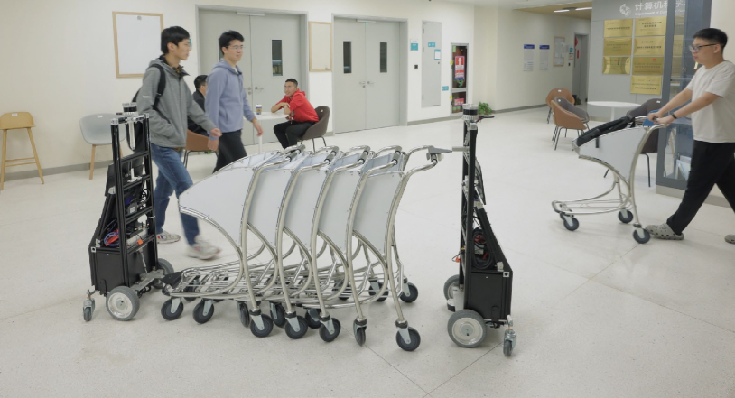
Figure 1: A snapshot showing a dual-robot system transporting a series of luggage trolleys in tandem in a dynamic environment.

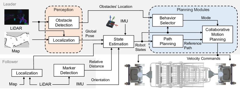
Figure 2: A diagram of our proposed navigation framework. It starts by measuring different sensory information, which is then processed by the perception module. Thereafter, the planning modules perform real-time computation and provide each robot with its velocity command.

II Related Work

Cooperative manipulation and transportation have been traditionally approached as a control task, where the desired trajectories of manipulated objects are often predefined[6]. The robots need to compute control inputs in a central or distributed fashion to enable the manipulated objects to track the desired trajectories or paths. A decentralized control framework is brought forth in [7], enabling robotic collaborative manipulation and transportation of large objects via separating locomotion and grasping. A number of works opt for the caging method [8, 9], in which the manipulated object stays in the interior of the formations formed by the robots. Without any explicit communication and with merely local measurements, the approach along with the physical system proffered in [10] realizes multi-robot cooperative object transportation via force coordination under a leader-follower paradigm. In [11], the authors provide a distributed adaptive control algorithm for several omnidirectional robots manipulating a rigid body to track a desired trajectory in $SE(3)$. However, these works all assume a priori known reference paths or trajectories and do not provide navigation solutions in dynamic environments. Moreover, control algorithms in [8, 9, 10, 11] are all designed for omnidirectional robots without nonholonomic constraints, making them unsuitable for many practical scenarios, such as the luggage trolley transportation work mentioned in this paper.

The advancement of onboard computing power has unlocked real-time deployment of optimization-based robot planning and control methods like model predictive control (MPC). In [12], the authors formulate the local control of manipulating deformable objects as a convex optimization problem and propose to solve it in a receding-horizon fashion with a centralized/distributed planning approach. Many studies have also investigated aerial cooperative payload carrying[13, 14] and connected vehicles[15, 16]. As expected, centralized optimization scales poorly with the number of robots. Thereupon, decentralized trajectory optimization methods keep drawing the field’s attention. The authors of [17] provide us with a decentralized MPC planning and control scheme for moving polygon objects with a set of omnidirectional robots on a plane. Though a distributed algorithm for optimization with separable variables is leveraged in multi-robot manipulation [18], it is not well-suited for multi-agent systems with highly nonlinear dynamics and strong couplings. Recent study have explored holonomically constrained collaborative locomotion [19] and their use in collaborative manipulation of cable-towed loads [20]. Nevertheless, none of the aforementioned approaches fits our task, which features tight coupling and complex constraints between robots, nonholonomic dynamics, and a demand for high motion precision.

Previous collaborative object transportation work in similar settings to ours has mainly focused on control. Yufka and Ozkan [21] take a formation-control perspective and propose a virtual leader-follower control scheme enabling multiple differential-drive robots to transport a pallet-like object. The work in [22] investigates a decentralized control algorithm for two nonholonomic robots without direct communication and provides thorough theoretic analyses. The authors of [23] employ risk-sensitive stochastic control for the same task, but only use this approach to compute one control input for a bi-robot system. Works in [21, 22, 23] all lack a systematic navigation solution that is essential for robots to perform the transportation task in complex, dynamic, and uncertain environments. The closest work to ours is, perhaps, [24]. The proposed approach allows for the integration of tracking control and obstacle avoidance. Nonetheless, the proposed method involves multiple handcrafted attractor functions and quite a few parameters that entail substantial fine tuning. In contrast, our hierarchical approach in this paper features algorithmic flexibility at different decision-making levels, and the parameter tuning is more intuitive and practical.

III System Description

III-A Framework Overview

We introduce an end-to-end autonomy framework for robotic collaborative trolley transportation in complex and dynamic environments. Our framework is illustrated in Fig. 2. For perception, multiple sensors are equipped to acquire both global and relative localization measurements, taking uncertainty into account. The proposed hierarchical decision-making module comprises three parts: i) the global path planner, ii) the behavior selector, and iii) the collaborative motion planner.

The three planning parts are built for three core objectives that ensure the safety and reliability of the trolley transportation task: kinematic-feasible trajectory generation, obstacle avoidance, and trolley array integrity maintenance. Starting with a 2D occupancy grid map, the global path planner provides a sequence of navigation waypoints by treating the entire robot-trolley assembly as a single virtual vehicle and considering kinematic constraints. Then, the collaborative motion planner computes online the two robots’ trajectories and velocity commands that track the reference path fed by the path planner and accounts for a variety of constraints, including nonholonomic dynamics, coupling formation constraints, and control bounds. The behavior selector evaluates the risk of collision with detected dynamic obstacles like pedestrians nearby, and adaptively adjusts the parameters of the motion planner or directly modifies the velocity commands if necessary. The advantage of such decomposition primarily resides in guaranteeing real-time performance for solving the complex planning and control problem with tight inter-agent couplings while still delivering precise and highly coordinated motions.

III-B Mechanical Design

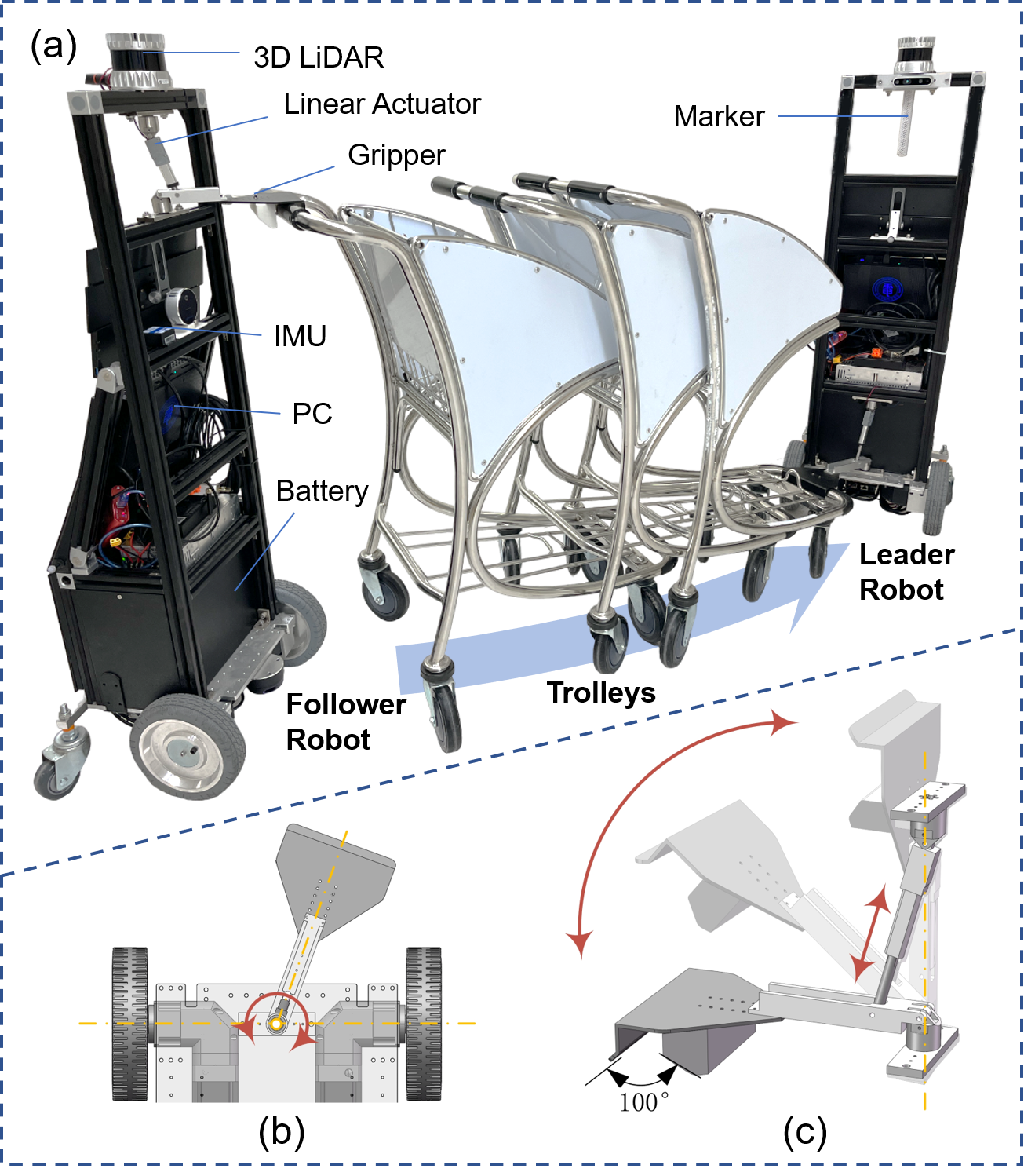
Figure 3: A prototype of the trolley collaborative transportation system is shown in Fig. 3(a), with the robot components labeled. Fig. 3(b) and (c) illustrate the structure and kinematics of the manipulator.

We develop a multi-robot system consisting of a leader and a follower for the collaborative trolley transportation task.

III-B1 Components

Adapted from the previous generation of luggage trolley collection robots [5], the leader and follower share a similar compact structure and identical components, including a differential-drive chassis with suspension, an aluminum alloy frame, large-capacity batteries, wiring, multiple sensors (LiDARs, cameras, IMU, etc. ), an onboard computer, and a manipulator, as shown in Fig. 3(a).

III-B2 Manipulator Design

The manipulator comprises a linear actuator and a gripper, which use leverage to grasp a trolley’s handler or beam, as depicted in Fig. 3(c). The manipulator’s placement is adjustable and dependent on the height of the handler or beam being gripped. To ensure that the gripper grasps the beam at the proper horizontal angle, the bottom of the manipulator must be at the same height as the beam. This placement provides a secure grip and acts as protection preventing axial forces on the linear actuator during transportation. As is shown in Fig. 3(a), the leader robot’s manipulator is at a low position gripping the front beam of the trolley, while the follower robot’s manipulator is positioned high to grip the handler.

To enable the two robots to transport trolleys collaboratively along curved paths, we employ a passive joint connecting the gripper and the robot, as shown in Fig. 3(b). By aligning the rotation axis of the gripper with that of the chassis, we eliminate the torque caused by the force exerted by the trolley queue on the gripper. This design effectively reduces the impact of the robots’ angular error and the dynamic adjustment required by the collaborative trolley transport system.

IV Methodology

In this section, we elaborate our hierarchical decision-making framework in three parts: the collaborative motion planner, the global path planner, and the behavior selector. In addition, we introduce how we fuse information from multiple sources for reliable state estimation.

IV-A Collaborative Motion Planning

The main challenge of the collaborative transportation task lies in the collaborative motion planning of the robot team. The robots need to compute their control inputs such that the robot-trolley assembly follows a desired path yielded by the global path planning module and meanwhile, to keep the trolleys sticking together and firmly attached to the robots. These requirements involve multiple constraints over the local collaborative motion planning problem. Therefore, we opt for a nonlinear model predictive control (NMPC) based approach. The NMPC framework provides great convenience for posing constraints, and has been successfully used in many robotic applications [25, 26]. In this section, we first describe the mathematical model of the robot-trolley system and then formulate an optimization problem for collaborative transportation motion planning.

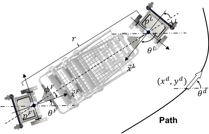
Figure 4: Illustration of the robot-trolley assembly tracking a reference path. The trolley stack is assumed to be one single rigid body.

The robot-trolley assembly consists of two differential-drive robots and an array of omnidirectional trolleys. Specifically, one robot $L$, a leader, is in charge of steering the trolleys at the head of the array, and a follower robot $F$ provides power and persists the formation configuration at the tail, as shown in Fig. 4. Assuming the trolleys are properly attached and the number of trolleys is known, we use the two robots’ planar positions and heading angles as the assembly system’s state and take the robots’ linear and angular velocities as the system’s input:

$$\mathbf{x} \triangleq\begin{bmatrix}x^{L}&y^{L}&\theta^{L}&x^{F}&y^{F}&\theta^{F}\end{bmatrix}^{\top}\in\mathbb{R}^{6},$$ (1)

$$\mathbf{u} \triangleq\begin{bmatrix}v^{L}&\omega^{L}&v^{F}&\omega^{F}\end{bmatrix}^{\top}\in\mathbb{R}^{4},$$ (2)

in which $\{L,F\}$ represents the role (“Leader” or “Follower”) of each robot. Thereupon, the assembly’s kinematics is formulated as two concatenated discrete-time unicycle model:

$$\mathbf{x}_{k+1}=f(\mathbf{x}_{k},\mathbf{u}_{k})=\mathbf{x}_{k}+\bm{G}(\mathbf{x}_{k})\mathbf{u}_{k},$$ (3)

where

$$\bm{G}(\mathbf{x}_{k})\triangleq\Delta t\begin{bmatrix}\cos\theta^{L}_{k}&0&0&0\\ \sin\theta^{L}_{k}&0&0&0\\ 0&1&0&0\\ 0&0&\cos\theta^{F}_{k}&0\\ 0&0&\sin\theta^{F}_{k}&0\\ 0&0&0&1\\ \end{bmatrix},$$

and $\Delta t$ is the sampling time interval. Herein, we further denote a number of variables derived from the state. The relative distance between the two robots is of great interest:

$$r\triangleq\|\mathbf{p}^{L}-\mathbf{p}^{F}\|,$$ (4)

where $\mathbf{p}^{i}\in\mathbb{R}^{2}$ for $i\in\{L,F\}$ is the planar position of a robot. Moreover, we denote the angle difference between the orientation of each robot and that of the vector that starts from the follower pointing at the leader as

$$\phi^{i}\triangleq\theta^{i}-\operatorname{arctan2}{\left(y^{L}-y^{F},x^{L}-x^{F}\right)},\quad i\in\{L,F\}.$$ (5)

Fig. 4 illustrates the geometrical relationships among these variables.

Remark 1

The desired relative distance $l$ between the two robots is a mapping $\kappa:\,N\to l$ with respect to the number of trolley(s) $N$. This quantity is assumed to be known a priori from previous trolley collection tasks, so it is a constant here.

Remark 2

As shown in Fig. 4, the center of the trolley stack does not necessarily coincide with the center of the line connecting the two robots. Under the condition that the trolleys are tightly arranged and the manipulators passively keep the same heading angle with the trolleys, we find that this slipping between manipulators and trolleys is negligible for motion planning in practice.

Now we pose the collaborative motion planning problem as an NMPC problem as follows:

$$\min_{\{\mathbf{x},\mathbf{u},\varepsilon\}}\quad J_{\text{T}}(\mathbf{x}_{T})+\sum^{T-1}_{k=0}J_{\text{S}}(\mathbf{x}_{k},\mathbf{u}_{k},\varepsilon_{k})$$ (6a)

s.t. $$\mathbf{x}_{k+1}=f(\mathbf{x}_{k},\mathbf{u}_{k})$$ (6b)

$$\mathbf{x}_{0}=\mathbf{x}_{\text{init}}$$ (6c)

$$|r_{k}-l|\leq\varepsilon_{k}$$ (6d)

$$\mathbf{x}_{k}\in\mathcal{X}$$ (6e)

$$\mathbf{u}_{k}\in\mathcal{U},$$ (6f)

where $J_{\text{T}}$ is the terminal cost, $J_{\text{S}}$ is the stage cost, and $\varepsilon_{k}$ is a slack variable.

The constraints are, from top to bottom, respectively: (6b) the kinematics constraint from (3); (6c) initial conditions; (6d) the relative distance constraint, relaxed by a slack variable to avoid infeasibility; (6e) workspace constraints; (6f) admissible control constraints, in which the robots’ velocities are bounded in the sense of $|v^{i}|\leq v_{\textrm{max}}^{i}$, and $|\omega_{i}|\leq\omega_{\textrm{max}}^{i}$, and accelerations are bounded via discretization as well $|{v}^{i}_{k+1}-v^{i}_{k}|\leq a^{i}_{\text{max}}$, $|\omega^{i}_{k+1}-\omega^{i}_{k}|\leq\alpha^{i}_{\text{max}}$.

The objective function (6a) contains several quadratic costs for path tracking and formation maintenance. Path tracking is achieved by employing a pure pursuit strategy encoded in the terminal cost:

$$J_{\text{T}}(\mathbf{x}_{T})=\left\|\mathbf{p}^{L}_{T}-\mathbf{p}^{L}_{\text{ref}}\right\|^{2}_{\bm{P}^{L}_{T}}+\left\|\mathbf{p}^{F}_{T}-\mathbf{p}^{F}_{\text{ref}}\right\|^{2}_{\bm{P}^{F}_{T}},$$ (7)

where $\|\mathbf{x}\|_{\bm{A}}\triangleq\sqrt{\mathbf{x}^{\top}\bm{A}\mathbf{x}}$. Reference positions $\mathbf{p}^{i}_{\textrm{ref}}$ are derived from the waypoints $\mathbf{q}^{d}_{n}=\begin{bmatrix}x^{d}_{n}&y^{d}_{n}&\theta^{d}_{n}\end{bmatrix}^{\top}$ for $n=0,1,\ldots$, produced by the global path planner via

$$\begin{cases}\begin{aligned} \mathbf{p}^{L}_{\textrm{ref}}&=\begin{bmatrix}x^{d}+\frac{l}{2}\cos{\theta^{d}}&y^{d}+\frac{l}{2}\sin{\theta^{d}}\end{bmatrix}^{\top}\\ \mathbf{p}^{F}_{\textrm{ref}}&=\begin{bmatrix}x^{d}-\frac{l}{2}\cos{\theta^{d}}&y^{d}-\frac{l}{2}\sin{\theta^{d}}\end{bmatrix}^{\top}.\end{aligned}\end{cases}$$ (8)

For stabilizing the formation of the robot team in order to keep the trolley stack’s integrity, we design the stage cost as

$$J_{\text{S}}(\mathbf{x}_{k})=\lambda^{r}_{k}\left|r^{2}_{k}-l^{2}\right|^{2}+\lambda^{\phi}_{k}\left(\phi^{F}_{k}\right)^{2}+\|\mathbf{u}_{k}\|^{2}_{\bm{R}_{k}}+w_{k}\varepsilon^{2}_{k}.$$ (9)

The first term intends to stabilize the distance to the desired value and contain the follower robot’s orientation to line up with the trolley array. The second term penalizes control efforts and the last term punishes the slack on the distance error. All coefficients $\bm{P}^{i}_{T},\,\bm{R}_{k},\,\lambda^{r}_{k},\,\lambda^{\phi}_{k},\,$, and $w_{k}$ are positive(-definite).

IV-B Global Path Planning

It is necessary to equip our system with a global path planner because the system is supposed to operate at potentially large-scale venues like international airports. To guarantee kinematic feasibility, we first model the robot-trolley assembly as a car-like virtual vehicle and then find an obstacle-free path given a 2D occupancy map of the operating environment. In this work, we define the reference path $\mathcal{D}\subset\mathbb{R}^{3}$ as a series of waypoints $\mathbf{q}^{d}_{n}\triangleq\begin{bmatrix}x^{d}_{n}&y^{d}_{n}&\theta^{d}_{n}\end{bmatrix}^{\top}$ for $n=0,1,\ldots$, representing desired planar positions and global orientations of the robot-trolley assembly.

The choice of the path planner is flexible, and we employ the Hybrid A^∗ planner [27] for simplicity. The adopted kinematics adapted from a bicycle model is as follows

$$\begin{cases}\begin{aligned} x_{k+1}&=x_{k}+v\Delta t\cos(\theta_{k}+\beta_{k})\\ y_{k+1}&=y_{k}+v\Delta t\sin(\theta_{k}+\beta_{k})\\ \theta_{k+1}&=\theta_{k}+\dfrac{v\cos\beta_{k}}{l}\Delta t\left(\tan\phi^{L}_{k}-\tan\phi^{F}_{k}\right)\\ \beta_{k}&=\arctan\left(\frac{1}{2}(\tan\phi^{L}_{k}+\tan\phi^{F}_{k})\right),\end{aligned}\end{cases}$$ (10)

where $\mathbf{q}=\begin{bmatrix}x&y&\theta\end{bmatrix}^{\top}$ is the 2D pose of a chosen reference point attached on the robot-trolley assembly, $v$ denotes the tangent velocity, $\phi^{L}$ and $\phi^{F}$ are the front and rear “steers” of the assembly, respectively, and $l$ is the desired distance between the two robots. To increase searching speed, we hold the tangent velocity $v$ as a reasonable constant, and let the planner uniformly sample feasible steer control $[\phi^{L},\phi^{F}]$ to extend the virtual vehicle’s poses between searching grids. The resulting path will serve as a sequence of waypoints and be sent to the motion planning module.

IV-C Behavior Selector

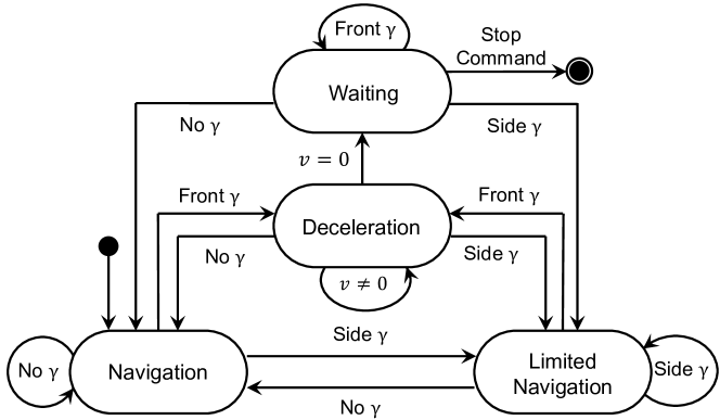
Figure 5: Finite-state automaton diagram of the behavior selector module. $\gamma$ represents the detected obstacle which is defined as 3 types by its position and determines the transitions between the 4 modes. The FSA starts in the Navigation mode and ends in the Waiting mode.

Operating in densely populated environments like international airports, the robotic system needs to ensure safety and must not bump into people. We identify that it is clumsy, unsafe, and even intimidating for the robots carrying a long array of trolleys to actively perform aggressive maneuvers for obstacle avoidance in such environments. In light of this finding, we propose a finite-state automaton (FSA) to manage the robots’ behaviors.

Concretely, we categorize the robots’ behaviors in four modes— Navigation, Deceleration, Waiting, and Limited Navigation— and each mode consists of a state in the proposed FSA as shown in Fig. 5. The transition between states depends on the relative position between the leader robot and detected dynamic obstacles in its vicinity. The region of interest (ROI) for dynamic obstacles detection covers an area $\mathcal{O}=\left\{\gamma=(\rho,\delta)\,\left|\,\rho\in\left[\underline{\rho},\overline{\rho}\right],\,\delta\in\left[\frac{\pi}{3},\frac{5\pi}{3}\right]\right.\right\}$, where $\gamma=(\rho,\delta)$ is the polar coordinate of a detected dynamic obstacle with the origin on the leader. When there is no dynamic obstacles in the ROI, i.e., $\forall\gamma\notin\mathcal{O}$, the robots are in the Navigation mode and the motion planner works as default. If obstacles are in the front blocking the robots’ way, that is, $\exists\gamma\in\mathcal{O}_{1}=\{\gamma\,|\,\delta\in\left[\frac{2\pi}{3},\frac{4\pi}{3}\right]\}$, the robots transit to the Deceleration mode and smoothly slow down for a stop. As the robots’ velocities gradually decrease to a neighborhood of $0$, the robots are in the Waiting state, making way for surrounding dynamic obstacles like humans. The Limited Navigation mode is activated for smooth braking and starting when the robots perceive humans on either side of the robot-trolley assembly ($\exists\gamma\in\mathcal{O}_{2}=\mathcal{O}\backslash\mathcal{O}_{1}\land\forall\gamma\notin\mathcal{O}_{1}$). In this mode, the robots move with a lower speed limit. The robots will switch back to Navigation if the detected humans move away, or enter Deceleration if any person moves from the side to the front.

IV-D State Estimation

It is of paramount importance to have reliable information on the robots’ states due to the demand for high motion precision for formation maintenance in this transportation task. As such, aside from using LiDARs, IMUs, and odometry for the localization of each individual robot, we have added markers on the leader robot so that we can measure the relative pose between the two robots from the follower with its LiDAR readings.

We adopt an extended Kalman filter (EKF) to fuse partial information coming from different sources: the localization modules on two robots and the relative pose measurement. The system’s discrete state-space representation is:

$$\begin{cases}\begin{aligned} \mathbf{x}_{k+1}&=f(\mathbf{x}_{k},\mathbf{u}_{k})=\mathbf{x}_{k}+\bm{G}(\mathbf{x}_{k})\mathbf{u}_{k}+\mathbf{v}_{k}\\ \mathbf{y}^{L}_{k+1}&=\bm{H}_{L}\mathbf{x}_{k+1}+\mathbf{w}^{L}_{k+1}\\ \mathbf{y}^{F}_{k+1}&=\bm{H}_{F}\mathbf{x}_{k+1}+\mathbf{w}^{F}_{k+1}\\ \mathbf{y}^{\Delta}_{k+1}&=\bm{H}_{\Delta}\mathbf{x}_{k+1}+\mathbf{w}^{\Delta}_{k+1},\end{aligned}\end{cases}$$ (11)

where

$$\bm{H}_{L}\triangleq\begin{bmatrix}\bm{I}_{3}&\bm{0}\end{bmatrix},\;\bm{H}_{F}\triangleq\begin{bmatrix}\bm{0}&\bm{I}_{3}\end{bmatrix},\;\bm{H}_{\Delta}\triangleq\begin{bmatrix}\bm{I}_{3}&-\bm{I}_{3}\end{bmatrix}.$$

$\mathbf{y}^{i}_{k}\in\mathbb{R}^{3}$ for $i\in\{L,F\}$ are pose measurements obtained from the robots’ localization modules; $\mathbf{y}^{\Delta}_{k}\in\mathbb{R}^{3}$ is a relative pose measurement. We assume that all noises follow zero-mean Gaussian distribution and are independent of one another, i.e., $\mathbf{v}_{k}\sim\mathcal{N}(\mathbf{0},\bm{V}_{k})$, $\mathbf{w}^{i}_{k}\sim\mathcal{N}(\mathbf{0},\bm{W}^{i}_{k})$ for $i\in\{L,F,\Delta\}$. Since we perform local motion planning in a centralized fashion, the prediction step is standard as that of any EKF. Measurements update at different frequencies, so we perform update steps asynchronously whenever an observation comes in. In practice, we find this fusion of multi-source information critical to the smooth functioning of the motion planner and facilitative of highly cooperative operation of the robots.

V Implementation and Experiments

We present experimental results to validate the effectiveness of the proposed collaborative motion planning module and demonstrate our trolley transportation system in complex and dynamic environments.

V-A Implementation Details

V-A1 Robot Setup

We use two autonomous robots to perform collaborative trolley transportation as mentioned in Section III-B. Our framework is implemented in Python and integrated through Robot Operating System (ROS Melodic). Each robot is equipped with an Intel NUC (specs: Core i7-1165G7 CPU@4.70GHz, 32GB RAM) to perform all computations online. Onboard sensors include an Ouster OS1 128-channel LiDAR and a 9-axis IMU. Both robots communicate through a wireless ad-hoc network with their onboard WiFi routers.

V-A2 Localization

Each robot runs its own global localization via AMCL [28] with a 2D occupancy map built a priori using GMapping [29]. For high-fidelity measurements of the robots’ relative position, we install a cylinder marker with unique reflectivity at the leader’s rotation center. The follower then extracts the marker’s position from the LiDAR scan points and takes it as the leader’s position.

V-A3 Planning

The global path planner is set up with $0.25$\mathrm{m}$\times 0.25$\mathrm{m}$\times 15^{\circ}$ resolution, and the virtual vehicle’s size is slightly expanded for safety. The motion planner runs at approximately $30$\mathrm{H}\mathrm{z}$$ with a horizon of $T=20$ steps, each discretized by $\Delta t=0.1$\mathrm{s}$$. The MPC problem is formulated by CasADi [30] and solved with IPOPT [31] on one robot’s onboard computer in real-time.

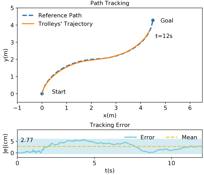
Figure 6: Results of the path tracking performance evaluation. The upper figure delineates the top view of the reference path and the trajectory of the reference point on the robot-trolley assembly till $t=12\,$\mathrm{s}$$. The lower figure plots the tracking error and related statistics over time. The shaded area represents the error’s $2\sigma$-margin.

V-B Collaborative Motion Planning Evaluation

To test the tracking performance of our collaborative motion planning method, we conduct a real-world experiment transporting three trolleys to track a given reference path in a motion capture area without obstacles. An OptiTrack motion capture system is used to provide precise localization feedback and validation. The reference path consists of 30 waypoints sampled from a concatenation of two arcs both with a $0.44\,$\mathrm{m}$^{-1}$ curvature.

The tracking results are shown in Fig. 6. In this experiment, we focus on the $X$-$Y$ position of a reference point attached on the robot-trolley assembly (in orange). The experiment starts at $(0,0)$ and the robots transport trolleys along the predefined reference path to the goal region with a center at $(4.5,4.2)$. The two robots accomplish the collaborative transportation task in $12.2$\mathrm{s}$$ with an average velocity of $0.491$\mathrm{m}\mathrm{/}\mathrm{s}$$, and stop when the distance to the goal is within $0.3$\mathrm{m}$$. Along the entire way, the tracking error is $2.77\pm 1.68$\mathrm{c}\mathrm{m}$$ with a maximal error of $5.66$\mathrm{c}\mathrm{m}$$.

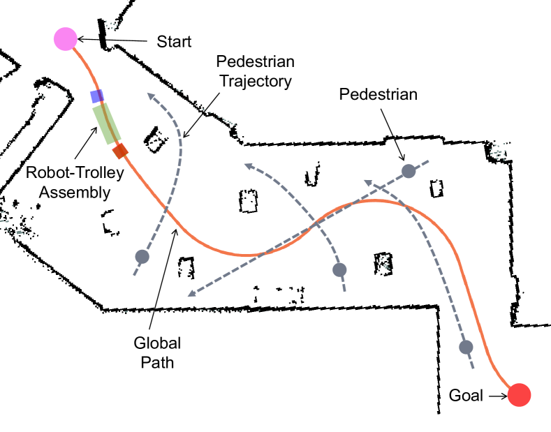
Figure 7: A top-view visualization illustrating our experiment setup. The global path is painted orange. Static obstacles in the occupancy map are represented by black points. The gray cylinders (circles in this figure) represent detected pedestrians and grey dotted lines denote their trajectories. The robots autonomously find the global path (orange curve) of the whole assembly and plan their own motions.

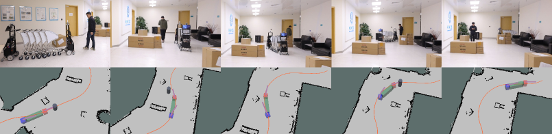
(a) Experiment of collaborative transportation of five trolleys in a cluttered narrow space.

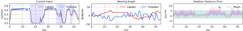
(b) Robots’ velocities, bearing angles, and the relative distance error in the cluttered narrow space.

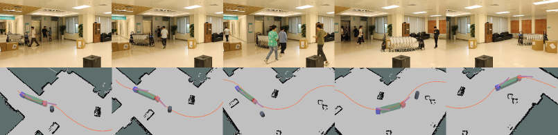
(c) Experiment of collaborative transportation of eight trolleys in presence of more pedestrians around.

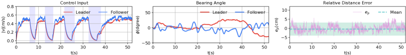
(d) Robots’ velocities, bearing angles, and the relative distance error in the populated space.

Figure 8: Snapshots and visualization of the proposed system working in two typical scenarios: narrow spaces and crowded spaces. In both scenarios, the visualization shows the robot-trolley assembly (green, blue, and red cubes), the global path (orange), the local motion plans of each robot (light purple), and the nearest detected pedestrian (gray cylinder). Three metrics of interest were also recorded: robots’ linear velocities, bearing angles, and the relative distance error. The light blue shades denote times when the behavior selector takes effect to yield for humans; light green shaded areas indicate the distance errors’ $2\sigma$-margins. The proposed framework clearly empowered our system to safely and smoothly perform collaborative trolley transportation tasks.

V-C Trolley Transportation Demonstration

To demonstrate the practical applicability of our proposed system for trolley transportation in real-world environments such as airports or supermarkets, we conduct experiments in complex and dynamic scenarios where the robots need to transport multiple trolleys while navigating through cluttered static obstacles and pedestrians. Fig. 7 illustrates the graphic representation of one experiment’s setup. As a result, the snapshots, the relevant data, and the visualization of the experiments are shown in Fig. 8.

V-C1 Narrow Space

In this scenario, the robots are collaboratively transporting 5 trolleys across a narrow space stuffed with 6 static obstacles and 3 pedestrians. The trolley stack is $1.98\,$\mathrm{m}$$ long and weighs around $100\,$\mathrm{k}\mathrm{g}$$. It is not easy even for an adult to manually handle a queue of more than five trolleys in such a complex environment.

As expected, the path planner successfully identifies a smooth global path, which is denoted as the orange curve in the visualization in Fig. 8(a). Although the obstacles result in a serpentine path with several turns almost to the robot-trolley assembly’s kinematic limit, the robots operate around their full speeds $v^{F}_{\text{max}}=0.7\,$\mathrm{m}\mathrm{/}\mathrm{s}$$, $v^{L}_{\text{max}}=0.6\,$\mathrm{m}\mathrm{/}\mathrm{s}$$ when the path is clear of dynamic obstacles. As pedestrians get in the way, the proposed behavior selector kicks in so the robots smoothly stop, firmly hold the trolleys for safety, and resume moving when the path gets clear, just as is shown in the shaded areas of the velocity plot in Fig. 8(b), starting at time $t\in\{15.8$\mathrm{s}$,36$\mathrm{s}$,46$\mathrm{s}$\}$, respectively.

Another critical requirement for successful transportation is to maintain the trolley array’s integrity, which is reflected by the relative pose of the two robots. Since the robots’ manipulators are not rigidly fixed on the trolleys, large variations in the relative distance or orientation difference between robots will cause detachment or structural damage. Deriving from the relative pose measured by the proposed LiDAR-marker detection method, Fig. 8(b) shows the error to the desired distance $e_{p}=1.49\pm 2.03\,$\mathrm{c}\mathrm{m}$$ and the difference between the orientation of the trolley stack and those of both robots are well kept within the range of $\pm 45^{\circ}$.

V-C2 Populated Space

This scenario involves two robots transporting 8 trolleys with a total length of $2.56\,$\mathrm{m}$$ in a broad hall filled with more moving humans. The velocity limits are set as $v^{F}_{\text{max}}=0.58\,$\mathrm{m}\mathrm{/}\mathrm{s}$$, $v^{L}_{\text{max}}=0.5\,$\mathrm{m}\mathrm{/}\mathrm{s}$$, and the acceleration is smaller. As presented in Fig. 8(c), the robot-trolley assembly successfully avoids all obstacles, makes way for several humans, tracks the reference path, and reaches the goal position. The fluctuations in the follower’s velocity depicted in Fig. 8(d) indicate the adjustment to keep the trolleys stuck tight. The relative distance error $e_{p}$ to the desired distance is $0.255\pm 2.36\,$\mathrm{c}\mathrm{m}$$.

These two experiments manifest the effectiveness of the proposed multi-robot system and demonstrate that our autonomy framework can provide highly cooperative motions despite a variety of underlying complex constraints for safe and smooth operation in collaborative trolley transportation.

VI Conclusions and Future Work

This paper presents a hierarchical navigation framework and integrates it into an autonomous multi-robot system designed for collaborative trolley transportation. By dividing the various inherent constraints and tackling them at different decision-making levels, our framework is robust and fast enough to provide real-time solutions for the challenging collaborative trolley transportation task. We demonstrate the proposed system to achieve cooperative trolley transportation in different scenarios. Experimental results have exhibited the efficacy and reliability of the proposed method and hardware system in cluttered and populated dynamic environments.

In the future, we will proceed with socially-aware motion planning and more large-scale outdoor realistic experiments. Moreover, we shall actively explore decentralized solutions of our framework to improve robustness and scalability.

References

- [1] C. Tang, J. Yu, W. Chen, B. Xia, and H. Zhang, “Relationship oriented semantic scene understanding for daily manipulation tasks,” in 2022 IEEE/RSJ International Conference on Intelligent Robots and Systems (IROS), 2022, pp. 9926–9933.
- [2] L. Johannsmeier and S. Haddadin, “A hierarchical human-robot interaction-planning framework for task allocation in collaborative industrial assembly processes,” IEEE Robotics and Automation Letters, vol. 2, no. 1, pp. 41–48, 2016.
- [3] A. Amanatiadis, C. Henschel, B. Birkicht, B. Andel, K. Charalampous, I. Kostavelis, R. May, and A. Gasteratos, “AVERT: An autonomous multi-robot system for vehicle extraction and transportation,” in 2015 IEEE International Conference on Robotics and Automation (ICRA), 2015, pp. 1662–1669.
- [4] J. Wang and M. Q.-H. Meng, “Real-time decision making and path planning for robotic autonomous luggage trolley collection at airports,” IEEE Transactions on Systems, Man, and Cybernetics: Systems, vol. 52, no. 4, pp. 2174–2183, 2021.
- [5] A. Xiao, H. Luan, Z. Zhao, Y. Hong, J. Zhao, W. Chen, J. Wang, and M. Q.-H. Meng, “Robotic autonomous trolley collection with progressive perception and nonlinear model predictive control,” in 2022 IEEE International Conference on Robotics and Automation (ICRA), 2022, pp. 4480–4486.
- [6] T. Elio, M. H. M. Alkilabi, and A. Otar, “Cooperative object transport in multi-robot systems: A review of the state-of-the-art,” Frontiers in Robotics and AI, vol. 5, p. 59, 2018.
- [7] T. Sugar and V. Kumar, “Control of cooperating mobile manipulators,” IEEE Transactions on Robotics and Automation, vol. 18, no. 1, pp. 94–103, 2002.
- [8] Z. Wang and V. Kumar, “Object closure and manipulation by multiple cooperating mobile robots,” in Proceedings 2002 IEEE International Conference on Robotics and Automation (Cat. No.02CH37292), vol. 1, 2002, pp. 394–399.
- [9] G. A. S. Pereira, M. F. M. Campos, and V. Kumar, “Decentralized algorithms for multi-robot manipulation via caging,” The International Journal of Robotics Research, vol. 23, no. 7-8, pp. 783–795, 2004.
- [10] Z. Wang, G. Yang, X. Su, and M. Schwager, “OuijaBots: Omnidirectional robots for cooperative object transport with rotation control using no communication,” in Distributed Autonomous Robotic Systems, 2018, vol. 6, pp. 117–131.
- [11] P. Culbertson, J.-J. Slotine, and M. Schwager, “Decentralized adaptive control for collaborative manipulation of rigid bodies,” IEEE Transactions on Robotics, vol. 37, no. 6, pp. 1906–1920, 2021.
- [12] J. Alonso-Mora, R. Knepper, R. Siegwart, and D. Rus, “Local motion planning for collaborative multi-robot manipulation of deformable objects,” in 2015 IEEE International Conference on Robotics and Automation (ICRA), 2015, pp. 5495–5502.
- [13] A. Tagliabue, M. Kamel, R. Siegwart, and J. Nieto, “Robust collaborative object transportation using multiple MAVs,” The International Journal of Robotics Research, vol. 38, no. 9, pp. 1020–1044, 2019.
- [14] B. E. Jackson, T. A. Howell, K. Shah, M. Schwager, and Z. Manchester, “Scalable cooperative transport of cable-suspended loads with UAVs using distributed trajectory optimization,” IEEE Robotics and Automation Letters, vol. 5, no. 2, pp. 3368–3374, 2020.
- [15] X. Liu, B. Luo, A. Abdo, N. Abu-Ghazaleh, and Q. Zhu, “Securing connected vehicle applications with an efficient dual cyber-physical blockchain framework,” in 2021 IEEE Intelligent Vehicles Symposium (IV). IEEE, 2021, pp. 393–400.
- [16] Q. Zhu, C. Huang, R. Jiao, S. Lan, H. Liang, X. Liu, Y. Wang, Z. Wang, and S. Xu, “Safety-assured design and adaptation of learning-enabled autonomous systems,” in Proceedings of the 26th Asia and South Pacific Design Automation Conference, 2021, pp. 753–760.
- [17] H. Ebel, W. Luo, F. Yu, Q. Tang, and P. Eberhard, “Design and experimental validation of a distributed cooperative transportation scheme,” IEEE Transactions on Automation Science and Engineering, vol. 18, no. 3, pp. 1157–1169, 2021.
- [18] O. Shorinwa and M. Schwager, “Scalable collaborative manipulation with distributed trajectory planning,” in 2020 IEEE/RSJ International Conference on Intelligent Robots and Systems (IROS), 2020, pp. 9108–9115.
- [19] J. Kim, R. T. Fawcett, V. R. Kamidi, A. D. Ames, and K. A. Hamed, “Layered control for cooperative locomotion of two quadrupedal robots: Centralized and distributed approaches,” arXiv preprint arXiv:2211.06913, 2022.
- [20] C. Yang, G. N. Sue, Z. Li, L. Yang, H. Shen, Y. Chi, A. Rai, J. Zeng, and K. Sreenath, “Collaborative navigation and manipulation of a cable-towed load by multiple quadrupedal robots,” IEEE Robotics and Automation Letters, vol. 7, no. 4, pp. 10 041–10 048, 2022.
- [21] A. Yufka and M. Ozkan, “Formation-based control scheme for cooperative transportation by multiple mobile robots,” International Journal of Advanced Robotic Systems, vol. 12, no. 9, p. 120, 2015.
- [22] A. Tsiamis, C. P. Bechlioulis, G. C. Karras, and K. J. Kyriakopoulos, “Decentralized object transportation by two nonholonomic mobile robots exploiting only implicit communication,” in 2015 IEEE International Conference on Robotics and Automation (ICRA), 2015, pp. 171–176.
- [23] S. Yasuda, T. Kumagai, and H. Yoshida, “Cooperative transportation robot system using risk-sensitive stochastic control,” in 2021 IEEE/RSJ International Conference on Intelligent Robots and Systems (IROS), 2021, pp. 5981–5988.
- [24] T. Machado, T. Malheiro, S. Monteiro, W. Erlhagen, and E. Bicho, “Multi-constrained joint transportation tasks by teams of autonomous mobile robots using a dynamical systems approach,” in 2016 IEEE International Conference on Robotics and Automation (ICRA), 2016, pp. 3111–3117.
- [25] A. Xiao, W. Tong, L. Yang, J. Zeng, Z. Li, and K. Sreenath, “Robotic guide dog: Leading a human with leash-guided hybrid physical interaction,” in 2021 IEEE International Conference on Robotics and Automation (ICRA), 2021, pp. 11 470–11 476.
- [26] Z. Jian, Z. Lu, X. Zhou, B. Lan, A. Xiao, X. Wang, and B. Liang, “PUTN: A plane-fitting based uneven terrain navigation framework,” in 2022 IEEE/RSJ International Conference on Intelligent Robots and Systems (IROS), 2022, pp. 7160–7166.
- [27] D. Dolgov, S. Thrun, M. Montemerlo, and J. Diebel, “Path planning for autonomous vehicles in unknown semi-structured environments,” The International Journal of Robotics Research, vol. 29, no. 5, pp. 485–501, 2010.
- [28] D. Fox, “KLD-sampling: Adaptive particle filters,” in Advances in Neural Information Processing Systems, vol. 14, 2001.
- [29] G. Grisetti, C. Stachniss, and W. Burgard, “Improved techniques for grid mapping with Rao-Blackwellized particle filters,” IEEE Transactions on Robotics, vol. 23, no. 1, pp. 34–46, 2007.
- [30] J. A. Andersson, J. Gillis, G. Horn, J. B. Rawlings, and M. Diehl, “CasADi: A software framework for nonlinear optimization and optimal control,” Mathematical Programming Computation, vol. 11, no. 1, pp. 1–36, 2019.
- [31] L. T. Biegler and V. M. Zavala, “Large-scale nonlinear programming using IPOPT: An integrating framework for enterprise-wide dynamic optimization,” Computers & Chemical Engineering, vol. 33, no. 3, pp. 575–582, 2009.