IFF: A Super-resolution Algorithm for Multiple Measurements

Abstract

We consider the problem of reconstructing one-dimensional point sources from their Fourier measurements in a bounded interval $[-\Omega,\Omega]$. This problem is known to be challenging in the regime where the spacing of the sources is below the Rayleigh length $\frac{\pi}{\Omega}$. In this paper, we propose a super-resolution algorithm, called Iterative Focusing-localization and Filtering (IFF), to resolve closely spaced point sources from their multiple measurements that are obtained by using multiple unknown illumination patterns. The new proposed algorithm has a distinct feature in that it reconstructs the point sources one by one in an iterative manner and hence requires no prior information about the source numbers. The new feature also allows for a subsampling strategy that can circumvent the computation of singular-value decomposition for large matrices as in the usual subspace methods. A theoretical analysis of the methods behind the algorithm is also provided. The derived results imply a phase transition phenomenon in the reconstruction of source locations which is confirmed in numerical experiments. Numerical results show that the algorithm can achieve a stable reconstruction for point sources with a minimum separation distance that is close to the theoretical limit. The algorithm can be generalized to higher dimensions.

I Introduction

In optical microscopy, super-resolution techniques are dedicated to improving the resolution of optical signals. The resolution, however, is limited by the band-limited optical transfer function, which is a consequence of the optical diffraction limit. This resolution limit can be characterized using the so-called Rayleigh limit or Rayleigh wavelength which simply depends on the cutoff frequency in the signal. In recent years, super-resolution techniques, either physical or computational or combined, are developed to break the conventional Rayleigh limit.

In this paper, we are interested in developing computational methods or algorithms for super-resolution problems. Roughly speaking, the methods to pursue super-resolution can be divided into two categories. The first one consists of optimization-based methods, such as TV minimization, atomic norm minimization, and B-LASSO, see [1][2][3][4][5][6] etc. Theoretical results show that these methods can provably reconstruct off-the-grid point sources from noisy measurements under the assumption that the minimum separation distance between the point sources is above several Rayleigh wavelengths. When the minimum separation distance is smaller than the Rayleigh wavelength, methods in the other category that are exemplified by MUltiple SIgnal Classification (MUSIC) [7], Matrix Pencil (MP) [8], and Estimation of Signal Parameters via Rotational Invariance Techniques (ESPRIT) [9], usually perform better. In literature, they are called subspace methods. The idea of subspace methods dates back to Prony’s method in 1795 [10]. In practice, these methods need prior information on the source number. We refer to [11][12][13][14][15][16][17][18] for theoretical grounds for the stability of subspace method and the discussions on computational resolution limit.

Intuitively, with multiple measurements that are obtained from multiple different illuminations, the accumulated information in the multiple measurements should contribute to a higher resolution. Indeed, subspace methods can take this advantage. In [19][20], a subspace method is applied to the aligned Hankel matrices to achieve better resolution. We also refer to [21] for the theoretical results. In this paper, we aim to propose a new super-resolution method/algorithm for multiple measurements. The method is motivated by the super-resolution techniques STED [22] and STORM [23]. We note that STED [22] achieves super-resolution by selectively deactivating fluorophores to minimize the illuminated area at the focal point, while STORM [23] breaks the Rayleigh limit by stochastically activating the individual photoactivatable fluorophores. The random one-by-one process inspires us to propose an iterative focusing-localization and filtering algorithm. We first numerically focus the illumination onto a single point source through an optimized linear combination of the available measurements and localize its position. We then filter the signal of the localized point source from the measurements. We repeat this focusing and filtering process until all point sources are reconstructed. A theoretical analysis of the method behind the algorithm is also provided.

I-A Problem Setup

In this paper, we consider the problem of reconstructing the locations of a collection of point sources from their multiple noisy measurements. Precisely, we consider the following mathematical model. Let $\mu=\sum_{j=1}^{n}a_{j}\delta_{y_{j}}$ be a discrete measure, where $y_{j}\in\mathbb{R},j=1,\cdots,n$, represent the supports of the point sources and $a_{j}\in\mathbb{C},j=1,\cdots,n$ their amplitudes.

The point sources are illuminated by multiple illumination patterns $I_{t}$, $1\leq t\leq T$, and the illuminated measures are

$$\mu_{t}=\sum_{j=1}^{n}I_{t}(y_{j})a_{j}\delta_{y_{j}},\ 1\leq t\leq T.$$

The measurements are the band-limited Fourier transform of the illuminated measures:

$${}Y_{t}\left(\omega\right) =\mathcal{F}\mu_{t}\left(\omega\right)+W_{t}\left(\omega\right)$$

$$=\sum_{j=1}^{n}I_{t}(y_{j})a_{j}e^{iy_{j}\omega}+W_{t}\left(\omega\right),\ 1\leq t\leq T.$$ (1)

where $\omega\in[-\Omega,\Omega]$, $\Omega$ is the cutoff frequency and $W_{t}\left(\omega\right)$ is the noise. Throughout, we assume that $T\geq n$ i.e., the number of measurements is larger than the number of sources. With slight abuse of notations, we also denote $\mathcal{F}\mu_{t}$ as the function $\mathcal{F}\mu_{t}\left(\omega\right),\ \omega\in[-\Omega,\Omega]$ and $\|f\|_{\infty}=\sup_{\omega}|f\left(\omega\right)|$. We assume that $\|W_{t}\left(\omega\right)\|_{\infty}<\sigma$ with $\sigma$ being the noise level. We denote

$$L=\left(\begin{matrix}I_{1}(y_{1})&\cdots&I_{1}(y_{n})\\ \vdots&&\vdots\\ I_{T}(y_{1})&\cdots&I_{T}(y_{n})\end{matrix}\right),$$

and call $L$ the illumination matrix. We observe that each row of $L$ represents an illumination pattern acting on different point sources while each column of $L$ represents different illuminations on a fixed point source.
After uniformly sampling over the interval $[-\Omega,\Omega]$ at sample points $\omega_{k}=\frac{k}{K}\Omega,k=-K,\cdots,K$, we align all the measurements into a matrix in the following form:

$$Y=\left(\begin{matrix}Y_{1}\left(\omega_{-K}\right)&\cdots&Y_{1}\left(\omega_{K}\right)\\ \vdots&&\vdots\\ Y_{T}\left(\omega_{-K}\right)&\cdots&Y_{T}\left(\omega_{K}\right)\end{matrix}\right).$$

We can calculate that

$${}Y=LAE+W,$$ (2)

where

$$A=\text{diag}\left(a_{1},\cdots,a_{n}\right),$$

$$E=\left(\begin{matrix}e^{iy_{1}\omega_{-K}}&\cdots&e^{iy_{1}\omega_{K}}\\ \vdots&&\vdots\\ e^{iy_{n}\omega_{-K}}&\cdots&e^{iy_{n}\omega_{K}}\end{matrix}\right),$$

and

$$W=\left(\begin{matrix}W_{1}\left(\omega_{-K}\right)&\cdots&W_{1}\left(\omega_{K}\right)\\ \vdots&&\vdots\\ W_{T}\left(\omega_{-K}\right)&\cdots&W_{T}\left(\omega_{K}\right)\end{matrix}\right).$$

Finally, we denote for a given measure $\nu$,

$$[\nu]=\left(\mathcal{F}\nu\left(\omega_{-K}\right),\mathcal{F}\nu\left(\omega_{-K+1}\right),\cdots,\mathcal{F}\nu\left(\omega_{K}\right)\right),$$

for ease of notation.

I-B Main contribution

In this paper, we are dedicated to developing a new super-resolution algorithm to reconstruct off-the-grid point sources from multiple noisy measurements. Unlike existing super-resolution algorithms that reconstruct all the point sources at once, the proposed method iteratively processes the following steps:

1. Achieve numerical source focusing by solving an optimization problem.

2. Localize the focused point source by using a subspace method.

3. Filter out the recovered source by using properly designed annihilating filters.

We summarize the proposed algorithm as iterative focusing-and-filtering-based source identification. This paper also provides a theoretical analysis of the methods behind IFF. Through the discussion, we observe several advantages of IFF:

• After the source focusing step, we only need to reconstruct a single source at each localization step. This fact allows us to deal with an optimization problem of rank-one Hankel matrices and thus allows the application of a subsampling strategy.

• IFF is a priori-free super-resolution method of high accuracy.

• IFF can achieve stable reconstruction for point sources with a minimum separation distance that is close to the theoretical limit.

I-C Organization of the paper

The paper is organized in the following way. In Section II and Section III, we explain the main ideas of source focusing and source filtering with theoretical discussion. The detailed implementation of the proposed algorithm can be found in Section IV. In Section V, we present numerical results of the algorithm. We conclude the paper with a discussion on future research topics in Section VI.

II Source Focusing and Localization

This section is dedicated to the first part of the proposed algorithm, namely source focusing and localization. We begin with introducing the idea of the source focusing. In Section II-A, we discuss the change of SNR resulting from source focusing. The design of the source focusing algorithm is proposed in Section II-B. Finally, a theoretical analysis of the method behind is given in Section II-C.

We first introduce some concepts and notations that are used throughout the paper. We assume the illumination matrix, $L$, has linearly independent columns and we write it into column blocks as follows:

$$L=\left(\begin{matrix}\alpha_{1},\alpha_{2},\cdots,\alpha_{n}\end{matrix}\right).$$

For $j=1,\cdots,n$, we define matrix $L_{j}$ as

$$L_{j}=\left(\begin{matrix}\alpha_{1},\cdots,\alpha_{j-1},\alpha_{j+1},\cdots,\alpha_{n}\end{matrix}\right).$$

We denote the projection map onto the column space of $L_{j}$ as $\mathcal{P}_{L_{j}}$ and the identity map as $\mathcal{I}$. From basic linear algebra, we know that $\mathcal{P}_{L_{j}}=L_{j}\left(L_{j}^{*}L_{j}\right)^{-1}L_{j}^{*}$.

We now consider focusing the illumination onto the $j$-th source $y_{j}$ by using linear combinations of the given measurements. For this purpose, we denote by $U_{j}$ the permutation matrix that permutes the $j$-th column with the $n$-th column. We rewrite (2) as follows:

$${}Y=LU_{j}\cdot U_{j}^{-1}AE+W.$$ (3)

Applying the QR decomposition to $LU_{j}$, we have

$${}LU_{j}=Q\left(\begin{matrix}R\\ 0\end{matrix}\right).$$ (4)

Multiplying $Q^{*}$ on the both sides of (3) yields

$${}Q^{*}Y=\left(\begin{matrix}R\\ 0\end{matrix}\right)U_{j}^{-1}AE+Q^{*}W.$$ (5)

We observe that the n-th row of $Q^{*}Y$ can then be regarded as the measurement generated by the single source $y_{j}$. Indeed, the $n$-th row of equation (5), denoted as $\tilde{Y}_{j}$, gives

$${}\tilde{Y}_{j} =\left(\sum_{t=1}^{T}q_{tn}Y_{t}\left(-K\right),\cdots,\sum_{t=1}^{T}q_{tn}Y_{t}\left(K\right)\right)$$

$$=R_{nn}a_{j}\left(e^{iy_{j}\omega_{-K}},\cdots,e^{iy_{j}\omega_{-K}}\right)$$ (6)

$$\ +\left(\sum_{t=1}^{T}q_{tn}W_{t}\left(-K\right),\cdots,\sum_{t=1}^{T}q_{tn}W_{t}\left(K\right)\right)$$

$$\triangleq\tilde{a}_{j}\left(e^{iy_{j}\omega_{-K}},\cdots,e^{iy_{j}\omega_{-K}}\right)+\tilde{W}_{j}.$$ (7)

We note that the component $\tilde{a}_{j}$, which depends on the permutation matrix $U_{j}$, gives an effective illumination amplitude on the $j$-th source while all the other sources are ”quenched” by the linear combination of given illumination patterns.

We can use the measurement from $\tilde{Y}_{j}$ to reconstruct the position of focused point source $y_{j}$ using a standard subspace method, such as MUltiple SIgnal Classification (MUSIC) and Matrix Pencil (MP). For this purpose, we form the following Hankel matrix for $\tilde{Y}_{j}$,

$$\tilde{H_{j}}=\left(\begin{matrix}\tilde{Y}_{j}\left(\omega_{-K}\right)&\tilde{Y}_{j}\left(\omega_{-K+1}\right)&\cdots&\tilde{Y}_{j}\left(\omega_{0}\right)\\ \tilde{Y}_{j}\left(\omega_{-K+1}\right)&\tilde{Y}_{j}\left(\omega_{-K+2}\right)&\cdots&\tilde{Y}_{j}\left(\omega_{1}\right)\\ \vdots&\vdots&&\vdots\\ \tilde{Y}_{j}\left(\omega_{0}\right)&\tilde{Y}_{j}\left(\omega_{1}\right)&\cdots&\tilde{Y}_{j}\left(\omega_{K}\right)\end{matrix}\right).$$ (8)

From (II), we see that $\tilde{H_{j}}$ is a linear combination of $\{H_{t}\}_{t=1}^{T}$ with coefficients $\{q_{tn}\}_{t=1}^{T}$, i.e.,

$$\tilde{H_{j}}=\sum_{t=1}^{T}q_{tn}H_{t}.$$ (9)

Here, the matrices $H_{t}$’s are the Hankel matrices associated with the given measurements $Y_{t}$’s in (I-A), i.e.

$${}H_{t}=\left(\begin{matrix}Y_{t}\left(\omega_{-K}\right)&Y_{t}\left(\omega_{-K+1}\right)&\cdots&Y_{t}\left(\omega_{0}\right)\\ Y_{t}\left(\omega_{-K+1}\right)&Y_{t}\left(\omega_{-K+2}\right)&\cdots&Y_{t}\left(\omega_{1}\right)\\ \vdots&\vdots&&\vdots\\ Y_{t}\left(\omega_{0}\right)&Y_{t}\left(\omega_{1}\right)&\cdots&Y_{t}\left(\omega_{K}\right)\end{matrix}\right),$$ (10)

for $1\leq t\leq T.$ It is important to notice that $\tilde{H_{j}}$ is the summation of a rank-one matrix and a noise matrix. We shall exploit this fact in our numerical reconstruction of the position of the focused point source. On the other hand, since the signal-to-noise ratio (SNR) plays a crucial role in the reconstruction of the subspace methods, we provide a theoretical analysis of the SNR for the focused measurement $\tilde{Y_{j}}$ in the next subsection.

II-A Discussion on SNR for the measurement of perfectly focusing

We start with the following estimation for each component of $\tilde{W}_{j}$ in equation (II):

$${}|\tilde{w}_{ij}|=|\sum_{n=1}^{T}q_{ni}W_{nj}|\leq\sqrt{\sum_{n=1}^{T}q_{ni}^{2}\cdot\sum_{n=1}^{T}W_{nj}^{2}}\leq\sqrt{T}\sigma.$$ (11)

We then consider $\tilde{a}_{j}$ in (II). It is clear that it depends on $R_{nn}$. We can calculate that

$${}R_{nn}=\|\left(\mathcal{I}-\mathcal{P}_{L_{j}}\right)\alpha_{j}\|_{2}.$$ (12)

Intuitively, the smaller $R_{nn}$ is, the lower SNR is and the more difficult the super-resolution problem is. The relationship between $R_{nn}$ and the illumination matrix $L$ can be illustrated through the following simple examples. First, we assume $L$ has a deficient row rank. In this case, we have $R_{nn}=0$. Without sufficient valid measurements, it is impossible to numerically focus on a single source. It also implies that adding the same measurement is not helpful since it cannot affect $R_{nn}$. Meanwhile, when $L$ has the same row vectors, the problem will degenerate to the single snapshot case. Then, let us consider the case when $L$ is diagonal. It is an ideal case where the sources are automatically focused in each illumination. In this case, $R_{nn}$ equals the illumination amplitude for the illumination onto the source $y_{j}$.
We now derive some quantitative characterization of $R_{nn}$. Under the assumption that the illumination matrix consists of independent and identically distributed random variables with mean $u$ and variance $v^{2}$, we have the following estimation for the second-order moment:

Proposition II.1.

For $R_{nn}$ given in (12), we have

$$\mathbb{E}\ R_{nn}^{2}\geq\left(T-n+1\right)v^{2}.$$ (13)

Especially, when $u=0$ and the components of $L$ are i.i.d. subgaussian random variables, we have the following concentration property for $R_{nn}$:

Proposition II.2.

For $u=0$ and $\|L_{ij}\|_{\psi_{2}}\leq B$, for any $t>0$, we have

$${}\mathbb{P} \left(|R_{nn}^{2}-\left(T-n+1\right)v^{2}|>t\right)$$

$$\quad\leq 2\exp{\left(-c\min\left(\frac{t^{2}}{B^{4}\left(T-n+1\right)},\frac{t}{B^{2}}\right)\right)},$$ (14)

where $c$ is some positive absolute constant and $\|\cdot\|_{\psi_{2}}$ is the subgaussian norm defined as

$$\|L_{ij}\|_{\psi_{2}}=\sup_{p\geq 1}p^{-1/2}\left(\mathbb{E}L_{ij}^{p}\right)^{1/p}.$$ (15)

In practice, the illumination amplitudes can be assumed to be bounded, i.e. the range of $L_{ij}$ is bounded. Under this assumption, the condition expressed by (15) is always met. As for the order of $R_{nn}$, we let $t=\frac{v^{2}}{2}\left(T-n+1\right)$, then the inequality (II.2) gives that $R_{nn}\sim O\left(\sqrt{T}\right)$ with probability $1-2e^{-O\left(T\right)}$. Combining this result with (11), we observe that under the assumption in Proposition II.2, numerical focusing via linear combination can preserve SNR with high probability if we use enough linearly independent measurements.

II-B Algorithm for focusing

We have shown in the previous discussion that with sufficiently many linearly independent illumination patterns, we can achieve a perfect illumination pattern that focuses on a single point source through a proper linear combination of the given measurements, see (9). We now address the issue of finding the linear combination coefficients $\{q_{tn}\}$’s numerically.

It is clear that a constant multiplier of $\tilde{Y}_{j}$ does not affect the SNR. In finding the linear combination coefficients, we do not need to apply additional constraints about the $\ell_{2}$-norm of $\left(q_{1,n},\cdots,q_{T,n}\right)$ though it is required to be one in QR decomposition. Let $N=\tilde{H}_{j}^{*}\tilde{H_{j}}$, we consider the following unconstrained optimization problem,

$${}\min_{q_{tn}}f\left(q_{1,n},\cdots,q_{Tn}\right):=\frac{Tr\left(N\right)^{2}}{Tr\left(N^{*}N\right)}.$$ (16)

We observe that $f\geq 1$ and $f=1$ if and only if $\tilde{H_{j}}$ is a rank-$1$ matrix. We point out that the objective function $f$ is determined only by the ratios of singular values. By maximizing the gap between the largest singular value and the rest, $f$ can reflect the low-rank nature better than traditional objective functionals which use the nuclear norm or other norms. Meanwhile, in the computation of $f$, there is no need for singular value decomposition. For the noiseless case, we observe that the solution to the optimization problem (16) is not unique and each solution corresponds to a perfect focusing on one of the point sources. In practice, with the presence of noise, we expect a solution to the optimization problem (16) can yield a good illumination pattern that is focused on a single point source in the sense that the contrast of the illumination amplitude on the focused point source and the others are sufficiently large so that the focused source can be distinguished and localized. The following estimate shed light on this issue.

Proposition II.3.

Let $\mu=\sum_{j=1}^{n}a_{j}\delta_{y_{j}}$, $Y=\mathcal{F}\mu\left(\omega\right)+W\left(\omega\right)$, where $\omega\in[-\Omega,\Omega]$ and $\|W\|_{\infty}<\sigma$. Let $H$ be the Hankel matrix generated by $Y$ and $N=H^{*}H$ be the normal matrix of $H$. Assume $|a_{s}|=\max_{j}|a_{j}|$, and $|a_{s}|>\sum_{t\neq s}|a_{t}|+\sigma$, then we have the following estimation:

$$\frac{Tr\left(N\right)^{2}}{Tr\left(N^{*}N\right)}\leq\left(\frac{|a_{s}|+\sum_{t\neq s}|a_{t}|+\sigma}{|a_{s}|-\sum_{t\neq s}|a_{t}|-\sigma}\right)^{4}.$$ (17)

In the next proposition, we derive an upper bound of the the minimization problem (16) when there is a single source with amplitude $M$ and noise level $\sigma$.

Proposition II.4.

Let $\mu=M\delta_{y}$, $Y=\mathcal{F}\mu\left(\omega\right)+W\left(\omega\right)$, where $\omega\in[-\Omega,\Omega]$, $\|W\|_{\infty}<\sigma$ and $M>2\sigma$. Let $H$ be the Hankel matrix generated by $Y$ and $N=H^{*}H$ be the normal matrix of $H$, then we have the following estimation:

$$\frac{Tr\left(N\right)^{2}}{Tr\left(N^{*}N\right)}\leq\left(1+4K\frac{\sigma^{2}}{M^{2}}\right)^{2}.$$ (18)

The upper bound in the proposition above can serve as a theoretical ground for the threshold we propose in the following. Note that $\sigma$ therein is the SNR after the focusing step which is not available in practice. We shall, nevertheless, use the original SNR as a good guess for it (see the discussion at the end of the previous subsection). We therefore set

$$\Gamma=\left(1+4K\left(\frac{1}{SNR}\right)^{2}\right)^{2}$$ (19)

as the threshold, where SNR represents the signal-to-noise ratio in the original problem. We reject all the solutions having function values larger than $\Gamma$. We call this step clean-up step. Notice that the solutions to the optimization problem (16) depend on the choice of initial guesses. With the equation (3) in our mind, we expect that the solutions may give us several clusters of positions. We then take an average over each cluster to get the recovered point sources $\{\hat{y}_{p}\}_{p=1}^{P}$. Clearly, $P\leq n$ here. The pseudo-code is given in Algorithm 1 below.

Input : Hankel matrices: $H_{t}$, $1\leq t\leq T$, Noise level: $\sigma$, Sampling number: $K$.

Input : Tolerance rate: $\epsilon$.

Initialization : Initial matrix: $I_{T\times T}$.

1 for $j\ =\ 1:T$ do

2       Initial data: $q^{\left(0\right)}[:,j]=I[:,j]$

3       Solve (16) to obtain $\{q_{tn}\}$ and $f\left(q_{1,n},\cdots,q_{Tn}\right)$ until $f\left(q_{1,n},\cdots,q_{Tn}\right)<1+\epsilon$. Get the result $q^{\left(r\right)}[:,j]$ and corresponding $\tilde{H}_{j}$

4       Apply MUSIC to $\tilde{H}_{j}$, get source estimation $\tilde{y}_{j}$.

5      

6Apply the clean-up step to the estimations and divide the results into several clusters. Take the average over each cluster to get the reconstructed sources $\{\hat{y}_{j}\}_{p=1}^{P}$. return $S=\{\hat{y}_{j}\}_{p=1}^{P}$

Algorithm 1 Source Focusing and Localization

We note that in Algorithm 1, $\Gamma$ is only used in (19) for the clean-up step but not the tolerance rate for the optimization problem. This is because the accuracy of the solution to (16) can significantly affect the accuracy of the recovered position of the selected source, while $\Gamma$ is derived in the ”worst-case scenario”. In practice, we need to choose a tolerance rate that is small enough. We believe that a more detailed analysis of the objective function $f$ may lead to a better choice of tolerance rate. We also notice that in Step 3, $\tilde{H_{j}}$ is the sum of a rank-one matrix and a noise matrix, which allows us to form the matrix $\tilde{H_{j}}$ with a small size to reconstruct the source position. This motivates us to develop a subsampling strategy, which will be discussed in Section IV. In Section III, we will see another advantage of the subsampling strategy.

II-C Analysis of the the numerical focusing and localization method

In this subsection, we analyze the reconstruction error of the numerical source focusing and localization method. We aim to address the following two issues: the first is under what conditions on the ground truth sources one step of source focusing and localization can reconstruct a source that is close to one of the ground truth sources. The second is the reconstruction error. It will be shown that the first issue is closely related to the minimum separation distance between the ground truth sources, which also set a theoretical limit for the method.

To proceed, we assume the ground truth point sources are supported at $\{y_{j}\}_{j=1}^{n}$. We denote the source obtained from numerical focusing and localization step as $\mu=M\delta_{y}$ with $M>0$. We write the numerically focused measurement as $\tilde{Y}=[\mu]+W^{\prime},$ where $W^{\prime}:=\tilde{Y}-[\mu]$. We assume that

$$\|W^{\prime}\|_{\infty}<\sigma^{\prime}$$

for some $\sigma^{\prime}>0$. In view of (II), we see that in the ideal focusing case, $M=|\tilde{a}_{j}|$, $\sigma^{\prime}\leq\sqrt{T}\sigma$. For convenience, we introduce the following definition.

Definition II.1.

Given a source $\mu$, we say a collection of point sources $\{\delta_{y_{j}}\}_{j=1}^{n}$ is $\sigma$-admissible to $\mu$ if there exist complex numbers $\hat{a}_{j},j=1,2,\cdots n$, such that $\hat{\mu}=\sum_{j=1}^{n}\hat{a}_{j}\delta_{y_{j}}$ satisfies

$$\|[\hat{\mu}]-[\mu]\|_{\infty}<\sigma.$$

We have the following theorem which shows that under certain minimum separation conditions to the ground truth sources, the focused source $\mu$ is close to one of the ground truth sources.

Theorem II.1.

Let $n\geq 2$, a collection of point sources $\{\delta_{y_{j}}\}_{j=1}^{n}$ is supported on $[-\frac{\pi}{2\Omega},\frac{\pi}{2\Omega}]$ satisfying the following condition:

$$\tau=\min_{p\neq q}|y_{p}-y_{q}|\geq\frac{3.03\pi e}{\Omega}\left(\frac{\sigma^{\prime}}{M}\right)^{\frac{1}{n}}.$$ (20)

If $\{\delta_{y_{j}}\}_{j=1}^{n}$ is $\sigma^{\prime}$-admissible to $\mu=M\delta_{y}$, then

$$\min_{1\leq j\leq n}|y-y_{j}|<\frac{\tau}{2}.$$

On the other hand, the proposition below shows that if the separation distance of the ground truth sources is below a certain threshold, then it is not guaranteed that the numerical-focused source is close to any of the ground truth sources.

Proposition II.5.

For given $0<\sigma^{\prime}<M$, and integer $n\geq 2$, let

$${}\tau=\frac{0.96e^{-\frac{3}{2}}}{\Omega}\left(\frac{\sigma^{\prime}}{M}\right)^{\frac{1}{n}}.$$ (21)

For uniformly separated point sources $\{\delta_{y_{j}}\}_{j=1}^{n}$ with distance $\tau$. There exist $y_{k}\in\{y_{j}\}_{j=1}^{n}$ such that $\mu=M\delta_{k}$, $\hat{\mu}=\sum_{j\neq k}\hat{a}_{j}\delta_{y_{j}}$ satisfying $\|[\mu]-[\hat{\mu}]\|_{\infty}<\sigma^{\prime}$.

Finally, we consider the reconstruction error. Under the assumption that a perfect focusing is achieved (see (II)), we have the following estimation.

Theorem II.2.

Let $\mu=M\delta_{y}$ be the focused point source supported on $[-\frac{\pi}{2\Omega},\frac{\pi}{2\Omega}]$. If $\{\delta_{y_{k}}\}$ is $\sigma^{\prime}$-admissible to $\mu$ for some $k$, then

$$|y-y_{k}|<\frac{\pi}{\Omega}\left(\frac{\sigma^{\prime}}{M}\right).$$ (22)

III Annihilating Filter Based Source Filtering

In this section, we propose an algorithm to remove the recovered point source/sources, which paves the way for a complete reconstruction.

III-A Source Filtering Algorithm

Literature usually uses the annihilating filters to achieve signal reconstruction, see [24] [20][25]. In contrast, we apply annihilating filters to remove the reconstructed point source/sources. To illustrate the idea, we first look at a toy example for the signal processed by an annihilating filter.

Example III.1.

Suppose we evenly sample a signal generated by a single point source with position $z$ and amplitude $a$, following the setup in section II. We have

$$Y=\left(ae^{iz\omega_{-K}},ae^{iz\omega_{-K+1}},\cdots,ae^{iz\omega_{K}}\right).$$ (23)

We then define a filter, $F$, by $F=\left(1,-e^{iz\frac{\Omega}{k}}\right)$. Calculating the discrete convolution of $Y$ and $F$, we derive

$$Y\ast F=\left(ae^{-iz\Omega},0,0,\cdots,0,-ae^{iz\frac{K+1}{K}\Omega}\right).$$ (24)

We observe that though there is a boundary effect due to discrete convolution, the middle part of $Y\ast F$ shows the complete filtering of the source. Based on this observation, we design the following annihilating filter for the original measurements:

$$F=\left(1,-e^{i\hat{y}_{1}\frac{\Omega}{K}}\right)\ast\left(1,-e^{i\hat{y}_{2}\frac{\Omega}{K}}\right)\ast\cdots\ast\left(1,-e^{i\hat{y}_{P}\frac{\Omega}{K}}\right),$$ (25)

where the convolution is in the discrete sense and $\{\hat{y}_{p}\}_{p=1}^{P}$ are derived in Algorithm 1. We denote $|\alpha|$ the length of the vector $\alpha$ and $\alpha[r:s]$ the vector that extracts the $r$-th to the $s$-th elements of $\alpha$. Notice that $|F|=P+1$ and $|Y\ast F|=2K+P+1$, the boundary effect occurs at the first $P$ elements and also the last $P$ elements of $Y_{t}\ast F$. We, therefore, pick the middle part as the processed measurements with the explicit form

$$Y_{t}^{\prime}=\left(Y_{t}\ast F\right)[P+1:2K+1],\quad t=1,\cdots,T.$$

The pseudo-code is given in Algorithm 2 below.

Input : Original measurements: $\{Y_{t}\}_{t=1}^{T}$, Recovered sources: $S=\{\hat{y}_{p}\}_{p=1}^{P}$.

1 Form the filter $F=\left(1,-e^{i\hat{y}_{1}\frac{\Omega}{K}}\right)\ast\cdots\ast\left(1,-e^{i\hat{y}_{P}\frac{\Omega}{K}}\right)$

2 for $t\ =\ 1:T$ do

3       Compute the discrete convolution $Y_{t}\ast F$

4       Let $Y^{\prime}_{t}=Y_{t}\ast F[P+1:2K+1]$.

5      

6return $\{Y_{t}^{\prime}\}_{t=1}^{T}$.

Algorithm 2 Source Filtering

III-B Analysis on SNR

In this subsection, we estimate the SNR of the signal obtained from the source filtering algorithm introduced in the previous subsection. The estimate will shed light on the reconstruction error for the next step. We first define $A_{j}$ by

$$A_{j}=\prod_{p=1}^{P}\left(e^{iy_{j}\frac{\Omega}{K}}-e^{i\hat{y}_{p}\frac{\Omega}{K}}\right),\ j=1,2,\cdots,n,$$ (26)

and $Q\left(x\right)$ by

$$Q\left(x\right) =\prod_{p=1}^{P}\left(x-e^{i\hat{y}_{p}\frac{\Omega}{K}}\right)\triangleq c_{0}+c_{1}x+\cdots+c_{P}x^{P}.$$ (27)

To write $Y^{\prime}$ more explicitly, we have

$${}Y_{t}^{\prime}\left(s\right)=\sum_{j=1}^{n}A_{j}a_{j}I_{t}(y_{j})e^{-iy_{j}\left(1-\frac{s}{K}\right)\Omega}+W^{\prime}\left(s\right),$$ (28)

for $s=0,1,\cdots,2K-P$. From (28) we see that both $\{A_{j}\}$ and $W^{\prime}$ affect the SNR after filtering, which leads us to analyze $\{A_{j}\}$ and $W^{\prime}\left(s\right)$ separately. For $W^{\prime}\left(s\right)$, we have the following worst-case estimation

$${}|W^{\prime}\left(s\right)| =|\sum_{l=0}^{P}c_{l}W\left(s+l\right)|\leq\sigma\sum_{l=0}^{P}|c_{l}|$$

$$=\sigma\sum_{l=0}^{P}|\sum_{\begin{subarray}{c}S\subset\{1,\cdots,P\}\\ |S|=l\end{subarray}}\prod_{p\in S}\left(-e^{i\hat{y}_{p}\frac{\Omega}{K}}\right)|$$

$$\leq\sigma\sum_{l=0}^{P}C_{P}^{l}=2^{P}\sigma.$$ (29)

For ${A_{j}}$, since $\{y_{j}\}$ are closely spaced and the sampling distance $\frac{\Omega}{K}$ is also small, we have the following estimation:

$${}|A_{j}| =\prod_{p=1}^{P}|e^{iy_{j}\frac{\Omega}{K}}-e^{i\hat{y}_{p}\frac{\Omega}{K}}|$$

$$=\prod_{p=1}^{P}\sqrt{2-2\cos\left(\left(y_{j}-\hat{y}_{p}\right)\frac{\Omega}{K}\right)}$$

$$\sim\left(\frac{\Omega}{K}\right)^{P}\prod_{p=1}|y_{j}-\hat{y}_{p}|.$$ (30)

We observe that in the ideal case, $y_{j}\in\{\hat{y}_{p}\}_{p=1}^{P}$, we will have $A_{j}=0$ which implies that the source positioned at $y_{j}$ is completely filtered out. Therefore, the accuracy of the source localization in Algorithm 1 plays an important role in the source filtering step. Inaccurate source filtering may cause additional errors. The results in (III-B) and (III-B) imply that the number of recovered sources and sampling distance have effects on SNR after filtering. We also notice that from (III-B), the subsampling strategy can reduce the effect due to the increased value of $\frac{\Omega}{K}$. In addition, the source filtering step reduces the number of point sources to be reconstructed in the next step. Both ensure that the iterative strategy of IFF to reconstruct all the point sources is achievable.

IV Implementation and Discussion

In this section, we present the implementation of the IFF algorithm, which combines Algorithm 1 and Algorithm 2. Meanwhile, we point out a rule for the choice of stopping criterion in the iterations and propose a subsampling strategy. We conclude this section with a discussion of the algorithm.

IV-A Details of Implementation

We first notice that we can achieve a complete reconstruction iteratively only with a proper stopping criterion. Naturally, the recovered source should be capable of generating all $T$ measurements with errors below the noise level. The stopping criterion can be defined as follows:

$$\max_{1\leq t\leq T}\min_{\hat{a}_{t,j}\in\mathbb{C}}\|[\hat{\mu}_{t}]-Y_{t}\|_{2}<\sqrt{2K+1}\sigma,$$ (31)

where $\hat{\mu_{t}}=\sum_{j=1}^{n}\hat{a}_{t,j}\delta_{j}$. We display the pseudo-algorithm for IFF algorithm in Algorithm 3.

Input : Sampling number: $K$, Original measurements: $\{Y_{t}\}_{t=1}^{T}$, noise level: $\sigma$.

Initialization : $S^{\left(0\right)}=\emptyset$, $\{Y_{t}^{\left(0\right)}\}=\{Y_{t}\}$, $r=0$.

1

2while $\gamma\geq\sqrt{2K+1}\sigma$ do

3       Proceed Algorithm 2 with input $\{Y_{t}\}$ and $S^{\left(r\right)}$, get the output $\{Y_{t}^{\left(r+1\right)}\}$

4       Let $s=\text{arg}\max_{m}\{s=2m-1,s\leq 2K-|S^{\left(r\right)}|+1\}$, form $s\times s$ Hankel matrices $\{H_{t}^{\left(r+1\right)}\}$ using $\{Y_{t}^{\left(r+1\right)}[1:2s-1]\}$

5       Proceed Algorithm 1 with input Hankel matrices $\{H_{t}^{\left(r+1\right)}\}$ and noise level $\sigma^{\left(r\right)}$, get the output $S^{\prime}$. Let $S^{\left(r+1\right)}=S^{\left(r\right)}\cup S^{\prime}$

6       $\gamma=\max_{1\leq t\leq T}\min_{\hat{a_{t,j}}}\|\mathcal{F}[\hat{\mu}_{t}]-Y_{t}\|_{2}$, where $\text{supp}\ \hat{\mu}_{t}=S^{\left(r+1\right)}$

7      

8return A set of reconstructed point sources: $S$

Algorithm 3 IFF Algorithm

We point out that in Algorithm 1, the input $\sigma^{\left(r\right)}$ should be adjusted in each iteration. This is mainly because of the change of SNR induced by annihilating filters, as discussed in Section III. Motivated by the estimation in Section III-B, one choice of $\sigma^{\left(r\right)}$ is

$$\sigma^{\left(r\right)}=C\left(\frac{\Omega}{Kd}\right)^{|S^{\left(r\right)}|}\sigma,$$

where $C$ is an order-one constant and $d$ is a prior guess for the cluster distance either based on the reconstruction result from step 3 in Algorithm 3 or other prior information. We point out that the choice of $\sigma^{(r)}$ can be flexible in practice.
Finally, we discuss the subsampling strategy mentioned in previous sections. We notice that Algorithm 1 may have a heavy computational cost if the size of the Hankel matrices is large. In the source localization step, however, we only need to handle nearly rank-one Hankel matrices due to the numerical focusing step. It motivates us to use a few sample points to form Hankel matrices. At the same time, the small size of Hankel matrices can also reduce the computational cost of the optimization problem. On the other hand, we observe that the size of Hankel matrices cannot be too small, otherwise, there may be some stability issues in the source localization. Therefore, a balanced subsampling strategy is needed to take into account the computational cost and the numerical instability in practice. Similar considerations also apply to Algorithm 2. On one hand, the application of annihilating filter can deteriorate the SNR, and a lower sampling rate is preferable for higher SNR, see (III-B). On the other hand, in the iterative construction of $Y_{t}$, the number of sample points should be sufficient to compensate for the boundary effect. Therefore, we uniformly subsample from $\{\omega_{k}\}$ to satisfy the minimum requirements on the sample size in practice.

IV-B Discussion of IFF Algorithm

In this subsection, we briefly discuss the IFF algorithm. First, we point out that from numerical experiments, the IFF algorithm is not sensitive to the choice of hyperparameters such as $\Gamma$ in Algorithm 1 and $\sigma^{(r)}$ in Algorithm 3. In the IFF algorithm, Algorithm 1 plays an essential role in the accuracy and efficiency of the whole method. It also assumes most of the computational power. The acceleration of Algorithm 1 can be achieved in the following ways. First, we notice that optimization problems for different initial guesses are mutually independent and thus can be solved parallelly. Second, techniques to accelerate the optimization algorithm can also be applied to improve both efficiency and accuracy.

We also remark that the IFF algorithm presented here is only suitable for the case of point sources in a small region, say of size less than or comparable to several Rayleigh lengths, and the number of measurements is great than the source number. For the general case of point sources in a large region and with multiscale structures, one can first decompose each measurement into “local measurements” that correspond to point sources in a small region or cluster, and then apply the IFF algorithm to each local measurement to reconstruct the point sources therein. The decomposition strategy will be introduced in a forthcoming paper.

In summary, IFF is an efficient algorithm that solves the local super-resolution problem with multiple measurements. We believe the idea can be generalized to other related problems.

V Numerical Experiments Result

In this section, we conduct two groups of numerical experiments to show the phase transition phenomenon and the numerical behavior.

V-A Phase Transition

We first introduce the super-resolution factor (SRF) which characterizes the ill-posedness of the super-resolution problem [1]. In the off-the-grid setting, SRF is defined by the ratio of Rayleigh limit and minimum separation distance. In our problem, the Rayleigh limit is $\frac{\pi}{\Omega}$ and the corresponding super-resolution factor is

$${}SRF:=\frac{\pi}{\Omega\tau},$$ (32)

where $\tau=\min_{p\neq j}|y_{p}-y_{j}|$.

For the super-resolution problem with multiple measurements, we notice that the worst case is that all the illumination patterns are linearly dependent and the measurements are essentially one measurement. In such a case, the computational resolution is of the order $O\left(\frac{\sigma}{m_{\min}}\right)^{\frac{1}{2n-1}}$, see [17]. Here, $m_{min}=\min_{j=1}|a_{j}|$. The best case is that each measurement is associated with a single “illuminated” source. Following the discussions in Section II-C, we predict that a phase transition phenomenon may occur. More precisely, we have demonstrated that a stable reconstruction is guaranteed if

$$\log\left(SNR\right)>\left(2n-1\right)\log\left(SRF\right)+\text{const}_{1},$$

and may fail if

$$\log\left(SNR\right)<n\log\left(SRF\right)+\text{const}_{2}.$$

Therefore, in the parameter space of $\log\left(SNR\right)-\log\left(SRF\right)$, there exist two lines with slopes $2n-1$ and $n$ respectively such that the cases above the former one are successfully reconstructed and the cases below the latter one are failed. As for the cases belonging to the intermediate region, the reconstruction result depends on the specifics of the illumination matrix. The phase transition is clearly illustrated in the numerical result below.

We set $\Omega=1$, and uniformly set 4 line spectra in $[-1,1]$ with separation distance $\tau$, amplitude $1$, and the noise level $\sigma$. We set the illumination matrix,$L$, consisting of independent and identically distributed random variables. We perform 1000 times experiments with random choices of $d$, $L$, and $\sigma$ to reconstruct the line spectra using Algorithm 3 and each time we use 10 measurements. Figure 1 shows the separation of the red points (successful reconstruction) and blue points (unsuccessful reconstruction) by two lines with slope $n$ and $2n-1$ respectively. The region in between is the phase transition region.

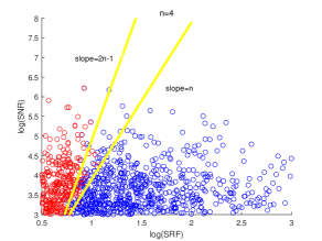
Figure 1: Plot of successful and unsuccessful point source reconstruction by Algorithm 3 in the parameter space $\log\left(SNR\right)-\log\left(SRF\right)$. Red one represents the successful case and the blue one represents the unsuccessful case.

V-B Reconstruction Behavior

To demonstrate the numerical reconstruction ability, we set $n=4$, $\Omega=1$, $\sigma=10^{-4}$ and

$$\mu=\delta_{y_{1}}+\delta_{y_{2}}+\delta_{y_{3}}+\delta_{y_{4}},$$

where $y_{1}=-0.75$, $y_{2}=-0.25$, $y_{3}=0.25$, $y_{4}=0.75$. For the illumination matrix, $L$, we set each element to be i.i.d. random variable that follows $\mathcal{U}[1,1+\sqrt{3}]$. Under this setup, we test the traditional subspace method using a single measurement. The result shows that the reconstructed source number is three, and the reconstructed source position is inaccurate. We perform 1000 random experiments using IFF algorithm (the randomness comes from the illumination and noise from the measurement). Each time, we use 10 measurements to reconstruct the line spectra’s position. The mean of position from 1000 experiments is $\left(\hat{y_{1}},\hat{y_{2}},\hat{y_{3}},\hat{y_{4}}\right)=\left(-0.7486,-0.2486,0.2481,0.7490\right)$. To compare with the standard method in multi-illumination LSE that align all the measurements and then apply the subspace method. We apply the standard method to the same data. The result shows the mean of position is $\left(\hat{y_{1}},\hat{y_{2}},\hat{y_{3}},\hat{y_{4}}\right)=\left(-0.7497,-0.2492,0.2493,0.7496\right)$. The variance of the two methods is both in the order $O\left(10^{-4}\right)$. Considering the noise level is $10^{-4}$, we claim the numerical behavior of Algorithm 3 is comparable to the standard method.

VI Conclusion

In this paper, we propose the IFF algorithm for the multiple measurements super-resolution problem in 1D and provide a theoretical analysis of the method behind it. We use two groups of experiments to illustrate the phase transition phenomenon and the numerical behavior respectively. With comparable numerical results to standard methods, the advantages of IFF algorithm can be summarized in the following two aspects. First, unlike standard subspace-method-based algorithms, the proposed one does not need prior information on the source number. Second, the subsampling strategy allows the reconstruction based on small-size Hankel matrices. The proposed algorithm may offer a new perspective in designing algorithms for super-resolution and other related problems. One may extend this method to higher dimensional super-resolution problems with multiple measurements.

VII Proofs of Results in Section II

VII-A Proof of Proposition II.3

First, we denote

$${}\phi_{s}\left(\omega\right)=\left(1,\omega,\omega^{2},\cdots,\omega^{s}\right).$$ (33)

We define $\mathcal{H}_{j}=a_{j}e^{-iy_{j}\Omega}\phi_{K}(e^{iy_{j}\frac{\Omega}{K}})\phi^{\top}_{K}(e^{iy_{j}\frac{\Omega}{K}})$ and $\hat{\mathcal{H}}_{j}=a_{j}\phi_{K}(e^{iy_{j}\frac{\Omega}{K}})\phi^{*}_{K}(e^{iy_{j}\frac{\Omega}{K}})$. It is easy to check that $\|\mathcal{H}_{j}\|_{2}=\|\mathcal{H}_{j}\|_{F}=\|\hat{\mathcal{H}}_{j}\|_{F}$.
Let $H$ be the Hankel matrix generated by $\mu$ as in (10). Clearly, $H$ has the following decomposition:

$$H=\sum_{j=1}^{n}\mathcal{H}_{j}+\left(\begin{array}[]{ccc}W_{-K}&\cdots&W_{0}\\ \vdots&&\vdots\\ W_{0}&\cdots&W_{K}\end{array}\right)\triangleq\sum_{j=1}^{n}\mathcal{H}_{j}+\Delta.$$ (37)

A straight-forward calculation gives

$$\|\hat{\mathcal{H}}_{j}\|_{F}^{2} =|a_{j}|^{2}Tr\left(\hat{\mathcal{H}^{*}_{j}}\hat{\mathcal{H}_{j}}\right)=|a_{j}|^{2}|\phi_{K}(e^{iy_{j}\frac{\Omega}{K}})|^{4}$$

$$=\left(K+1\right)^{2}|a_{j}|^{2}.$$ (38)

Notice that $H=\mathcal{H}_{s}+\sum_{t\neq s}\mathcal{H}_{t}+\Delta$. By Weyl’s theorem, we have

$$|\|H\|_{2}-\|\mathcal{H}_{s}\|_{2}| \leq\|\sum_{t\neq s}\mathcal{H}_{t}+\Delta\|_{2}\leq\|\sum_{t\neq s}\mathcal{H}_{t}+\Delta\|_{F}$$

$$\leq\sum_{t\neq s}\|\mathcal{H}_{t}\|_{F}+\|\Delta\|_{F}$$

$$\leq\left(K+1\right)\left(\sum_{t\neq s}|a_{t}|+\sigma\right).$$ (39)

Therefore

$$\|H\|_{2} \geq\|\mathcal{H}_{s}\|_{2}-\left(K+1\right)\left(\sum_{t\neq s}|a_{t}|+\sigma\right)$$

$$=\left(K+1\right)\left(|a_{s}|-\sum_{t\neq s}|a_{t}|-\sigma\right).$$ (40)

On the other hand,

$$\|H\|_{F} \leq\sum_{j=1}^{n}\|\mathcal{H}_{j}\|_{F}+\|\Delta\|_{F}$$

$$=\left(K+1\right)\left(|a_{s}|+\sum_{t\neq s}|a_{t}|+\sigma\right).$$ (41)

Combining the above two inequalities, we have

$$\frac{Tr\left(N\right)^{2}}{Tr\left(N^{*}N\right)} \leq\left(\frac{\|H\|_{F}}{\|H\|_{2}}\right)^{4}$$

$$\leq\left(\frac{|a_{s}|+\sum_{t\neq s}|a_{t}|+\sigma}{|a_{s}|-\sum_{t\neq s}|a_{t}|-\sigma}\right)^{4}.$$ (42)

VII-B Proof of Proposition II.4

Similar to the argument in the proof of Proposition II.3, we write

$$H =M\left(\begin{array}[]{ccc}e^{iy\omega_{-K}}&\cdots&e^{iy\omega_{0}}\\ \vdots&&\vdots\\ e^{iy\omega_{0}}&\cdots&e^{iy\omega_{K}}\end{array}\right)$$ (46)

$$\quad\quad+\left(\begin{array}[]{ccc}W_{-K}&\cdots&W_{0}\\ \vdots&&\vdots\\ W_{0}&\cdots&W_{K}\end{array}\right)$$ (50)

$$\triangleq X+\Delta.$$ (51)

Step 1.
We list the singular values of $H$ in a descending order as:

$$\hat{\sigma}_{1}\geq\hat{\sigma}_{2}\geq\cdots\geq\hat{\sigma}_{K+1}.$$

Similarly, we list the singular values of $X$:

$$\sigma_{1}\geq\sigma_{2}\geq\cdots\geq\sigma_{K+1}.$$

A straight-forward calculation shows that

$${}\sigma_{1}=M\left(K+1\right),\ \ \sigma_{j}=0,\ j\geq 2.$$ (52)

By Weyl’s theorem, for $1\leq j\leq K+1$, we have

$${}|\hat{\sigma}_{j}-\sigma_{j}|\leq\|\Delta\|_{2}\leq\|\Delta\|_{F}\leq\left(K+1\right)\sigma.$$ (53)

Step 2.
Define $r_{j}=\frac{\hat{\sigma}_{j}}{\hat{\sigma}_{1}}$ for $1\leq j\leq K+1$. Combining (52) and (53), we have

$$r_{j}\leq\frac{\sigma}{M-\sigma}\leq\frac{2\sigma}{M},\ 2\leq j\leq K+1.$$ (54)

By the fact that the function $g\left(t\right):=\frac{\left(1+t\right)^{2}}{1+t^{2}}$ is increasing on interval $\left(0,1\right)$, we have

$$\frac{Tr\left(N\right)^{2}}{Tr\left(N^{*}N\right)} =\frac{\left(\sum_{j=1}^{K+1}\hat{\sigma}^{2}_{j}\right)^{2}}{\sum_{j=1}^{K+1}\hat{\sigma}^{4}_{j}}=\frac{\left(\sum_{j=1}^{K+1}r^{2}_{j}\right)^{2}}{\sum_{j=1}^{K+1}r^{4}_{j}}$$

$$\leq\left(1+4K\frac{\sigma^{2}}{M^{2}}\right)^{2}.$$ (55)

VII-C Proof of Proposition II.1

Denote $1_{T}=\left(1,1,\cdots,1\right)^{\top}\in\mathbb{C}^{T}$ and let $Q_{j}=I_{T\times T}-L_{j}\left(L_{j}^{*}L_{j}\right)^{-1}L_{j}^{*}$.
It is easy to see that for each $1\leq j\leq T$, $Q_{j}$ is a positive semi-definite projection matrix with $Tr\left(Q_{j}\right)=T-n+1$, $\|Q_{j}\|_{2}=1$ and $\|Q_{j}\|_{F}^{2}=Tr\left(Q_{j}^{*}Q_{j}\right)=Tr\left(Q_{j}\right)=T-n+1$.
Therefore for each $j=1,2,\cdots,T$, we have

$${}\mathbb{E}\|\left(I-\mathcal{P}_{j}\right)\alpha_{j}\|_{2}^{2} =\mathbb{E}\left(\alpha_{j}^{*}{Q_{j}^{*}}{Q_{j}}\alpha_{j}\right)$$

$$=\mathbb{E}\left(\mathbb{E}\left(\alpha_{j}^{*}{Q_{j}^{*}}Q_{j}\alpha_{j}|Q_{j}\right)\right)$$

$$=\mathbb{E}\left(\mathbb{E}\left(Tr\left(\alpha_{j}^{*}{Q_{j}^{*}}Q_{j}\alpha_{j}\right)|Q_{j}\right)\right)$$

$$=v^{2}\mathbb{E}\left(Tr\left(Q_{j}\right)u^{2}+1_{T}^{*}Q_{j}1_{T}\right)$$

$$\geq\left(T-n+1\right)v^{2}.$$ (56)

VII-D Proof of Proposition II.2

From the argument of the proof of Proposition II.1, when $u=0$, we have

$$\mathbb{E}\ R_{nn}^{2}=\left(T-n+1\right)v^{2}.$$ (57)

Combining the equality above and the Hanson-Wright inequality [26], we obtain the desired result.

VII-E Proof of Theorem II.1

We only give the proof for $n$ is even, the case when $n$ is odd can be proved in a similar way.
Step 1.
Let

$${}2K+1=\left(n+1\right)r+q,$$ (58)

where $r,\ q$ are nonnegative integers with $r\geq 1$ and $0\leq q<n+1$. We denote $\theta_{j}=y_{j}\frac{r\Omega}{K}$, $j=1,\cdots,n$. For $y_{j}\in[-\frac{\pi}{2\Omega},\frac{\pi}{2\Omega}]$, in view of (58), it is clear that

$$\theta_{j}=y_{j}\frac{r\Omega}{K}\in[-\frac{\pi}{2},\frac{\pi}{2}],\ \ \ j=1,\cdots,n.$$ (59)

We write $\tau^{\prime}=\tau\frac{r\Omega}{K}$ to be the minimum separation distance between $\{\theta_{j}\}$, define $\mathcal{S}=\{y\in[-\frac{\pi}{2\Omega},\frac{\pi}{2\Omega}],\min_{j}|y-y_{j}|\geq\frac{\tau}{2}\}$, $\mathcal{S^{\prime}}=\{\theta\in[-\frac{\pi}{2},\frac{\pi}{2}],\min_{j}|\theta-\theta_{j}|\geq\frac{\tau^{\prime}}{2}\}$.
Step 2.
For $\hat{\mu}=\sum_{j=1}^{n}\hat{a}_{j}\delta_{y_{j}}$, we notice that

$$[\hat{\mu}]-[\mu] =\left(\mathcal{F}\hat{\mu}\left(\omega_{-K}\right),\mathcal{F}\hat{\mu}\left(\omega_{-K+1}\right),\cdots,\mathcal{F}\hat{\mu}\left(\omega_{K}\right)\right)^{\top}$$

$$\quad-\left(\mathcal{F}\mu\left(\omega_{-K}\right),\mathcal{F}\mu\left(\omega_{-K+1}\right),\cdots,\mathcal{F}\mu\left(\omega_{K}\right)\right)^{\top},$$ (60)

where $\omega_{-K}=-\Omega$, $\omega_{-K+1}=-\Omega+h$, $\cdots$, $\omega_{K}=\Omega$ and $h=\frac{\Omega}{K}$. In what follows, We denote the partial measurement as $\omega_{r,t}=-\Omega+trh$, $0\leq t\leq n$. We then have

$$\left(\mathcal{F}\hat{\mu}\left(\omega_{r,0}\right),\mathcal{F}\hat{\mu}\left(\omega_{r,1}\right),\cdots,\mathcal{F}\hat{\mu}\left(\omega_{r,n}\right)\right)^{\top}$$

$$\quad-\left(\mathcal{F}\mu\left(\omega_{r,0}\right),\mathcal{F}\mu\left(\omega_{r,1}\right),\cdots,\mathcal{F}\mu\left(\omega_{r,n}\right)\right)^{\top}$$

$$=B_{1}\hat{a}-M\tilde{B}_{1},$$ (61)

where

$$\hat{a}=\left(\hat{a_{1}},\hat{a_{2}},\cdots,\hat{a_{n}}\right)^{\top},$$

$$\tilde{B}_{1}=\left(e^{iy\omega_{r,0}},e^{iy\omega_{r,1}},\cdots,e^{iy\omega_{r,n}}\right),$$

and

$$B_{1}=\left(\begin{array}[]{ccc}e^{iy_{1}\omega_{r,0}}&\cdots&e^{iy_{n}\omega_{r,0}}\\ e^{iy_{1}\omega_{r,1}}&\cdots&e^{iy_{n}\omega_{r,1}}\\ \vdots&\vdots&\vdots\\ e^{iy_{1}\omega_{r,n}}&\cdots&e^{iy_{n}\omega_{r,n}}\end{array}\right)$$ (66)

It is clear that

$${}\min_{\hat{a}\in\mathbb{C}^{n},y\in\mathcal{S}}\|[\hat{\mu}]-[\mu]\|_{\infty} \geq\min_{\hat{a}\in\mathbb{C}^{n},y\in\mathcal{S}}\|B_{1}\hat{a}-M\tilde{B}_{1}\|_{\infty}$$

$$\geq\frac{1}{\sqrt{n+1}}\min_{\hat{a}\in\mathbb{C}^{n},y\in\mathcal{S}}\|B_{1}\hat{a}-M\tilde{B}_{1}\|_{2}.$$ (67)

Step 3.
Let $\theta=y\frac{r\Omega}{K}\in[-\frac{\pi}{2},\frac{\pi}{2}]$ and $\phi_{s}\left(\omega\right)=\left(1,\omega,\omega^{2},\cdots,\omega^{s}\right)$ defined as in (33).
Notice that

$$B_{1}= \left(\phi_{n}(e^{i\theta_{1}}),\phi_{n}(e^{i\theta_{2}}),\cdots,\phi_{n}(e^{i\theta_{n}})\right)$$

$$\quad\cdot\text{diag}\left(e^{-iy_{1}\Omega},e^{-iy_{2}\Omega},\cdots,e^{-iy_{n}\Omega}\right).$$ (68)

We have

$$\min_{\hat{a}\in\mathbb{C}^{n},y\in\mathcal{S}}\|B_{1}\hat{a}-M\tilde{B}_{1}\|_{2}=\min_{\hat{a}\in\mathbb{C}^{n},y\in\mathcal{S}}\|D_{1}\hat{a}-\tilde{M}\tilde{D}_{1}\|_{2},$$ (69)

where $D_{1}=\left(\phi_{n}\left(e^{i\theta_{1}}\right),\phi_{n}\left(e^{i\theta_{2}}\right),\cdots,\phi_{n}\left(e^{i\theta_{n}}\right)\right)$, $\tilde{D}_{1}=\phi_{n}\left(e^{i\theta}\right)$, $\tilde{M}=e^{-iy\Omega}M$.
Step 4.
By Theorem 3.1 in [17] and Stirling’s formula, we have

$$\min_{\hat{a}\in\mathbb{C}^{n},y\in\mathcal{S}}\|D_{1}\hat{a}-\tilde{M}\tilde{D}_{1}\|_{2}\geq\min_{\theta\in\mathcal{S^{\prime}}}\ \frac{M}{2^{n}}|\prod_{j=1}^{n}\left(e^{i\theta}-e^{i\theta_{j}}\right)|$$

$$\geq\min_{\theta\in\mathcal{S^{\prime}}}\ \frac{M}{\pi^{n}}\prod_{j=1}^{n}|\theta-\theta_{j}|$$

$$\quad\left(\text{by $|e^{i\theta}-e^{i\theta_{j}}|\geq\frac{2}{\pi}|\theta-\theta_{j}|$, for all $\theta,\theta_{j}\in[-\frac{\pi}{2},\frac{\pi}{2}]$}\right)$$

$$=\frac{M}{\pi^{n}}\left(\frac{\tau^{\prime}}{2}\right)^{n}\left(n-1\right)!\quad\left(\text{by Lemma \ref{lem_2}}\right)$$

$$\geq M\left(\frac{\Omega}{\pi}\right)^{n}\frac{\left(n-1\right)!}{\left(n+1\right)^{n}}\frac{\tau^{n}}{2^{n}}\quad\left(\text{by $\frac{r\Omega}{K}\geq\frac{\Omega}{n+1}$}\right)$$

$$\geq M\left(\frac{\Omega}{\pi}\right)^{n}\frac{\tau^{n}}{2^{n}}\frac{1}{e^{n}}\left(\frac{n-1}{n+1}\right)^{n}\sqrt{\frac{2\pi e^{2}}{n-1}}.$$ (70)

Step 5.
Combining (VII-E), (69) and (VII-E), we have

$$\min_{\hat{a}\in\mathbb{C}^{n},y\in\mathcal{S}}\|[\hat{\mu}]-[\mu]\|_{\infty}\geq\frac{M\left(\Omega\tau\right)^{n}}{\left(2e\pi\right)^{n}}\left(\frac{n-1}{n+1}\right)^{n}\sqrt{\frac{2\pi e^{2}}{n^{2}-1}}.$$ (71)

By the separation distance condition in (20) and the inequality that $\frac{2\left(n+1\right)}{n-1}\left(\frac{n^{2}-1}{2\pi e}\right)^{\frac{1}{2n}}<3.03$, we have

$$\min_{\hat{a}\in\mathbb{C}^{n},y\in\mathcal{S}}\|[\hat{\mu}]-[\mu]\|_{\infty}\geq\sigma^{\prime}.$$ (72)

It then follows that if $\{\delta_{y_{j}}\}_{j=1}^{n}$ is $\sigma^{\prime}$-admissible to $\mu$ then $\mu$ need to be within the $\frac{\tau}{2}$-neighborhood of $\{\delta_{y_{j}}\}_{j=1}^{n}$.

VII-F Proof of Proposition II.5

We only give the proof for $n$ is even, the case when $n$ is odd can be proved in a similar way. We write $n=2p$.
Step 1.
Let

$$\tau=\dfrac{0.96e^{-\frac{3}{2}}}{\Omega}\left(\frac{\sigma^{\prime}}{M}\right)^{\frac{1}{n}}$$ (73)

and $y_{1}=-p\tau$, $y_{2}=-\left(p-1\right)\tau$, $\cdots$, $y_{p}=-\tau$, $y_{p+1}=0$, $\cdots$, $y_{2p+1}=p\tau$. Consider the following linear system

$${}Aa=0,$$ (74)

where $A=\left(\phi_{2p-1}\left(t_{1}\right),\cdots,\phi_{2p-1}\left(t_{2p+1}\right)\right)$. Since this linear system is underdetermined and $A$ has full column rank, there exists a solution whose elements are all nonzero real numbers. By a scaling of $a$, we can assume that $|a_{k}|=\min_{1\leq j\leq 2p+1}|a_{j}|=M$.
We define $\hat{\mu}=\sum_{j\neq k}a_{j}\delta_{y_{j}}$, $\mu=-a_{k}\delta_{y_{k}}$ and show $\|[\hat{\mu}]-[\mu]\|_{\infty}\leq\sigma^{\prime}$ next.
Step 2.
Observe that

$$\|[\mu]-[\mu]\|_{\infty}\leq\max_{\omega\in[-\Omega,\Omega]}|\mathcal{F}\gamma\left(\omega\right)|,$$ (75)

where $\gamma=\sum_{j=1}^{2p+1}a_{j}\delta_{y_{j}}$ and

$${}\mathcal{F}\gamma\left(\omega\right) =\sum_{j=1}^{2p+1}a_{j}e^{iy_{j}\omega}=\sum_{j=1}^{2p+1}a_{j}\sum_{k=0}^{\infty}\frac{\left(iy_{j}\omega\right)^{k}}{k!}$$

$$=\sum_{k=0}^{\infty}Q_{k}\left(\gamma\right)\frac{\left(i\omega\right)^{k}}{k!},$$ (76)

where $Q_{k}\left(\gamma\right)=\sum_{j=1}^{2p+1}a_{j}y_{j}^{k}$. By (74), we have $Q_{k}\left(\gamma\right)=0$ for $0\leq k\leq 2p-1$. We then estimate $Q_{k}\left(\gamma\right)$ for $k\geq 2p$.
Step 3.
We reorder $a_{j}$’s in the following way

$$M=|a_{j_{1}}|\leq|a_{j_{2}}|\leq\cdots\leq|a_{j_{2p+1}}|.$$ (77)

From (74), we derive that

$$a_{j_{1}}\phi_{2p-1}\left(y_{j_{1}}\right)= \left(\phi_{2p-1}\left(y_{j_{2}}\right),\cdots,\phi_{2p-1}\left(y_{j_{2p+1}}\right)\right)$$

$$\quad\cdot\left(-a_{j_{2}},\cdots,-a_{j_{2p+1}}\right)^{\top},$$ (78)

and hence

$$a_{j_{1}}\left(\phi_{2p-1}\left(y_{j_{2}}\right),\cdots,\phi_{2p-1}\left(y_{j_{2p+1}}\right)\right)^{-1}\phi_{2p-1}\left(y_{j_{1}}\right)$$

$$\quad=\left(-a_{j_{2}},\cdots,-a_{j_{2p+1}}\right)^{\top}.$$ (79)

By Lemma $3.5$ in [17], we have

$$a_{j_{2p+1}}=-a_{j_{1}}\prod_{2\leq q\leq 2p}\frac{y_{j_{1}}-y_{j_{q}}}{y_{j_{2p+1}}-y_{j_{q}}}.$$ (80)

Therefore

$$|a_{j_{2p+1}}|\leq\frac{\left(2p\right)!}{p!\cdot p!}|a_{j_{1}}|\leq 2^{2p}M,$$ (81)

and consequently

$$\sum_{j=1}^{2p+1}\left|a_{j}\right|=\sum_{q=1}^{2p+1}\left|a_{j_{q}}\right|\leq\left(2p+1\right)2^{2p}M.$$ (82)

Then for $k\geq 2p$,

$$|Q_{k}\left(\gamma\right)| =|\sum_{j=1}^{2n-1}a_{j}y_{j}^{k}|\leq\sum_{j=1}^{2p+1}|a_{j}|\left(p\tau\right)^{k}$$

$$\leq\left(2p+1\right)2^{2p}M\left(p\tau\right)^{k}.$$ (83)

Step 4.
Using (VII-F), we have

$$|\max_{\omega\in[-\Omega,\Omega]}\mathcal{F}\gamma\left(\omega\right)| \leq\sum_{k\geq 2p}\left(2p+1\right)2^{2p}M\left(p\tau\right)^{k}\frac{\Omega^{k}}{k!}$$

$$<\frac{\left(2p+1\right)2^{2p}M\left(p\tau\Omega\right)^{2p}}{\left(2p\right)!}\sum_{k=0}^{+\infty}\frac{\left(p\tau\Omega\right)^{k}}{k!}$$

$$=\frac{\left(2p+1\right)2^{2p}M\left(p\tau\Omega\right)^{2p}}{\left(2p\right)!}e^{p\tau\Omega}$$

$$\leq\frac{\left(2p+1\right)M}{2\sqrt{\pi p}}\left(e\tau\Omega\right)^{2p}e^{p\tau\Omega}$$

$$\quad\left(\text{by Lemma \ref{lem_3}}\right)$$

$$\leq\frac{\left(2p+1\right)M}{2\sqrt{\pi p}}\left(e\tau\Omega\right)^{2p}e^{p}.$$ (84)

The last inequality is because (21) implies $\tau\Omega\leq 1$. Finally, using (21) and the inequality that $0.96^{2p}\frac{2p+1}{2\sqrt{\pi p}}\leq 1$, we have

$$\max_{\omega\in[-\Omega,\Omega]}|\mathcal{F}\gamma\left(\omega\right)|\leq\sigma^{\prime},$$

which completes the proof.

VII-G Proof of Theorem II.2

Let $d=\frac{\pi}{\Omega}\left(\frac{\sigma^{\prime}}{M}\right),$ and $\mathcal{S}=\{z\in[-\frac{\pi}{2\Omega},\frac{\pi}{2\Omega}],|z-y|\geq d\}$.
For $\hat{\mu}=a\delta_{z}$, we have

$$[\hat{\mu}]-[\mu] =\left(\mathcal{F}\hat{\mu}\left(\omega_{-K}\right),\mathcal{F}\hat{\mu}\left(\omega_{-K+1}\right),\cdots,\mathcal{F}\hat{\mu}\left(\omega_{K}\right)\right)^{\top}$$

$$\quad-\left(\mathcal{F}\mu\left(\omega_{-K}\right),\mathcal{F}\mu\left(\omega_{-K+1}\right),\cdots,\mathcal{F}\mu\left(\omega_{K}\right)\right)^{\top}$$

$$=a\left(e^{iz\omega_{-K}},\cdots,e^{iz\omega_{K}}\right)^{\top}$$

$$\quad-M\left(e^{iy\omega_{-K}},\cdots,e^{iy\omega_{K}}\right)^{\top}.$$ (85)

where $\omega_{-K}=-\Omega$, $\omega_{-K+1}=-\Omega+h$, $\cdots$, $\omega_{K}=\Omega$ and $h=\frac{\Omega}{K}$. Then, we have

$$\min_{a\in\mathbb{C},z\in\mathcal{S}}\|[\hat{\mu}]-[\mu]\|_{\infty}$$

$$\quad=\min_{a\in\mathbb{C},z\in\mathcal{S}}\|a\left(e^{iz\omega_{-K}},1\right)^{\top}-M\left(e^{iy\omega_{-K}},1\right)^{\top}\|_{\infty}$$

$$\quad\geq\frac{1}{\sqrt{2}}\min_{a\in\mathbb{C},z\in\mathcal{S}}\|a\left(e^{iz\omega_{-K}},1\right)^{\top}-M\left(e^{iy\omega_{-K}},1\right)^{\top}\|_{2}$$

$$\quad=\frac{M}{2}\min_{z\in\mathcal{S}}|e^{iy\Omega}-e^{iz\Omega}|\quad(\text{by Theorem 3.1 in \cite[cite]{[\@@bibref{}{9410626}{}{}]}})$$

$$\quad\geq Md\frac{\Omega}{\pi}$$

$$\quad\quad(\text{by $|e^{i\theta}-e^{i\hat{\theta}}|\geq\frac{2}{\pi}|\theta-\hat{\theta}|$, for $\theta,\hat{\theta}\in[-\frac{\pi}{2},\frac{\pi}{2}]$})$$

$$\quad\geq\sigma^{\prime}.$$ (86)

Therefore, $|z-y|<d$ is a necessary condition.

VIII Appendix

Lemma VIII.1.

Let $-\frac{\pi}{2}\leq\theta_{1}<\theta_{2}<\cdots<\theta_{n}\leq\frac{\pi}{2}$ with $\lambda=\min_{i\neq j}|\theta_{s}-\theta_{t}|$. Let $\mathcal{S}=\{\theta\in[-\frac{\pi}{2},\frac{\pi}{2}],\min_{j}|\theta-\theta_{j}|\geq d\}$, where $d\leq\frac{\lambda}{2}$. Then, we have

$$\min_{\theta\in\mathcal{S}}\prod_{j=1}^{n}|\theta-\theta_{j}|\geq\frac{\left(n-1\right)!}{2^{n-1}}\cdot d\cdot\lambda^{n-1}.$$

Proof.

We only prove the case n is even, the case $n$ is odd can be similarly proved.
Let $\mathcal{S^{\prime}}=\{\theta\in[\theta_{1},\theta_{n}],\min_{j}|\theta-\theta_{j}|\geq d\}$. Clearly, we have

$$\min_{\theta\in\mathcal{S}}\prod_{j=1}^{n}|\theta-\theta_{j}|=\min_{\theta\in\mathcal{S^{\prime}}}\prod_{j=1}^{n}|\theta-\theta_{j}|$$

Assume the minimum is achieved at $\theta^{*}\in\left(\theta_{p},\theta_{p+1}\right)$, for some $p$, where $1\leq p\leq n-1$. Denote $x=\theta^{*}-\theta_{p}\in[d,\theta_{p+1}-\theta_{p}-d]$. We then have

$$\min_{\theta\in\mathcal{S^{\prime}}}\prod_{j=1}^{n}|\theta-\theta_{j}|= x\left(\lambda+x\right)\left(2\lambda+x\right)\cdots\left(\left(p-1\right)\lambda+x\right)$$

$$\quad\cdot\left(\lambda-x\right)\cdots\left(\left(n-p\right)\lambda-x\right)\triangleq P\left(x\right).$$

It is easy to check that $P\left(x\right)\geq P\left(\theta_{p+1}-\theta_{p}-d\right)$ when $2p\leq n$, and $P\left(x\right)\geq P\left(d\right)$ when $2p\geq n$.
For $2p\geq n$, which implies $p\geq\frac{n}{2}$:

$$P\left(x\right)\geq P\left(d\right) =d\left(\lambda+d\right)\left(2\lambda+d\right)\cdots\left(\left(p-1\right)\lambda+d\right)$$

$$\quad\quad\cdot\left(\lambda-d\right)\cdots\left(\left(n-p\right)\lambda-d\right)$$

$$\geq d\cdot\left(p-1\right)!\lambda^{p-1}\cdot\frac{\left(2\left(n-p\right)-1\right)!!}{2^{n-p}}\lambda^{n-p}$$

$$\geq d\lambda^{n-1}\frac{\left(2T-2\right)!!\left(2T-1\right)!!}{2^{n-1}}$$

$$\geq d\lambda^{n-1}\frac{\left(n-1\right)!}{2^{n-1}}$$

By symmetry, we can derive the same result for $p\leq\frac{n}{2}$. ∎

Lemma VIII.2.

For $n\geq 1$, we have

$$\frac{n^{2n}}{\left(2n\right)!}\leq\frac{1}{2\sqrt{\pi}}\left(\frac{e}{2}\right)^{2n}$$ (87)

Proof.

By the following Stirling approximation:

$${}\sqrt{2\pi}n^{n+\frac{1}{2}}e^{-n}\leq n!\leq en^{n+\frac{1}{2}}e^{-n}.$$ (88)

we have

$$\frac{n^{2n}}{\left(2n\right)!}\leq\frac{n^{2n}}{\sqrt{2\pi}\left(2n\right)^{2n+\frac{1}{2}}e^{-2n}}=\frac{1}{2\sqrt{\pi}}\left(\frac{e}{2}\right)^{2n}.$$

∎

References

- [1] E. J. Candès and C. Fernandez-Granda, “Towards a mathematical theory of super-resolution,” Communications on Pure and Applied Mathematics, vol. 67, no. 6, pp. 906–956, 2014.
- [2] E. J. Candès and C. Fernandez-Granda, “Super-resolution from noisy data,” Journal of Fourier Analysis and Applications, vol. 19, no. 6, pp. 1229–1254, 2013.
- [3] G. Tang, B. N. Bhaskar, and B. Recht, “Near minimax line spectral estimation,” IEEE Transactions on Information Theory, vol. 61, no. 1, pp. 499–512, 2014.
- [4] Y. Chi and M. F. Da Costa, “Harnessing sparsity over the continuum: Atomic norm minimization for superresolution,” IEEE Signal Processing Magazine, vol. 37, no. 2, pp. 39–57, 2020.
- [5] V. Duval and G. Peyré, “Exact support recovery for sparse spikes deconvolution,” Foundations of Computational Mathematics, vol. 15, no. 5, pp. 1315–1355, 2015.
- [6] J.-M. Azaïs, Y. de Castro, and F. Gamboa, “Spike detection from inaccurate samplings,” Applied and Computational Harmonic Analysis, vol. 38, no. 2, pp. 177–195, 2015.
- [7] R. Schmidt, “Multiple emitter location and signal parameter estimation,” IEEE Transactions on Antennas and Propagation, vol. 34, no. 3, pp. 276–280, 1986.
- [8] Y. Hua and T. K. Sarkar, “Matrix pencil method for estimating parameters of exponentially damped/undamped sinusoids in noise,” IEEE Transactions on Acoustics, Speech, and Signal Processing, vol. 38, no. 5, pp. 814–824, 1990.
- [9] R. Roy and T. Kailath, “Esprit-estimation of signal parameters via rotational invariance techniques,” IEEE Transactions on Acoustics, Speech, and Signal Processing, vol. 37, no. 7, pp. 984–995, 1989.
- [10] R. Prony, “Essai expérimental et analytique,” J. de l’ Ecole Polytechnique (Paris), vol. 1, no. 2, pp. 24–76, 1795.
- [11] D. Batenkov, G. Goldman, and Y. Yomdin, “Super-resolution of near-colliding point sources,” Information and Inference: A Journal of the IMA, 05 2020. iaaa005.
- [12] W. Li and W. Liao, “Stable super-resolution limit and smallest singular value of restricted fourier matrices,” Applied and Computational Harmonic Analysis, vol. 51, pp. 118–156, 2021.
- [13] W. Li, W. Liao, and A. Fannjiang, “Super-resolution limit of the esprit algorithm,” arXiv preprint arXiv:1905.03782, 2019.
- [14] D. L. Donoho, “Superresolution via sparsity constraints,” SIAM journal on mathematical analysis, vol. 23, no. 5, pp. 1309–1331, 1992.
- [15] L. Demanet and N. Nguyen, “The recoverability limit for superresolution via sparsity,” arXiv preprint arXiv:1502.01385, 2015.
- [16] A. Moitra, “Super-resolution, extremal functions and the condition number of vandermonde matrices,” in Proceedings of the Forty-seventh Annual ACM Symposium on Theory of Computing, STOC ’15, (New York, NY, USA), pp. 821–830, ACM, 2015.
- [17] P. Liu and H. Zhang, “A theory of computational resolution limit for line spectral estimation,” IEEE Transactions on Information Theory, vol. 67, no. 7, pp. 4812–4827, 2021.
- [18] P. Liu and H. Zhang, “A mathematical theory of the computational resolution limit in one dimension,” Applied and Computational Harmonic Analysis, vol. 56, pp. 402–446, 2022.
- [19] J. Min, K. H. Jin, M. Unser, and J. C. Ye, “Grid-free localization algorithm using low-rank hankel matrix for super-resolution microscopy,” IEEE Transactions on Image Processing, vol. 27, no. 10, pp. 4771–4786, 2018.
- [20] K. H. Jin, D. Lee, and J. C. Ye, “A general framework for compressed sensing and parallel mri using annihilating filter based low-rank hankel matrix,” IEEE Transactions on Computational Imaging, vol. 2, no. 4, pp. 480–495, 2016.
- [21] P. Liu, S. Yu, O. Sabet, L. Pelkmans, and H. Ammari, “Mathematical foundation of sparsity-based multi-illumination super-resolution,” arXiv preprint arXiv:2202.11189, 2022.
- [22] S. W. Hell, “Toward fluorescence nanoscopy,” Nature Biotechnology, vol. 21, pp. 1347–1355, Nov. 2003.
- [23] M. J. Rust, M. Bates, and X. Zhuang, “Sub-diffraction-limit imaging by stochastic optical reconstruction microscopy (STORM),” Nat Methods, vol. 3, pp. 793–795, Aug. 2006.
- [24] M. Vetterli, P. Marziliano, and T. Blu, “Sampling signals with finite rate of innovation,” IEEE Transactions on Signal Processing, vol. 50, no. 6, pp. 1417–1428, 2002.
- [25] G. Ongie and M. Jacob, “Off-the-grid recovery of piecewise constant images from few fourier samples,” SIAM Journal on Imaging Sciences, vol. 9, no. 3, pp. 1004–1041, 2016.
- [26] M. Rudelson and R. Vershynin, “Hanson-wright inequality and sub-gaussian concentration,” Electronic Communications in Probability, vol. 18, pp. 1–9, 2013.