Iterative Geometry Encoding Volume for Stereo Matching

Abstract

Recurrent All-Pairs Field Transforms (RAFT) has shown great potentials in matching tasks. However, all-pairs correlations lack non-local geometry knowledge and have difficulties tackling local ambiguities in ill-posed regions. In this paper, we propose Iterative Geometry Encoding Volume (IGEV-Stereo), a new deep network architecture for stereo matching. The proposed IGEV-Stereo builds a combined geometry encoding volume that encodes geometry and context information as well as local matching details, and iteratively indexes it to update the disparity map. To speed up the convergence, we exploit GEV to regress an accurate starting point for ConvGRUs iterations. Our IGEV-Stereo ranks $1^{st}$ on KITTI 2015 and 2012 (Reflective) among all published methods and is the fastest among the top 10 methods. In addition, IGEV-Stereo has strong cross-dataset generalization as well as high inference efficiency. We also extend our IGEV to multi-view stereo (MVS), i.e. IGEV-MVS, which achieves competitive accuracy on DTU benchmark. Code is available at https://github.com/gangweiX/IGEV.

1 Introduction

Inferring 3D scene geometry from captured images is a fundamental task in computer vision and graphics with applications ranging from 3D reconstruction, robotics and autonomous driving. Stereo matching which aims to reconstruct dense 3D representations from two images with calibrated cameras is a key technique for reconstructing 3D scene geometry.

Many learning-based stereo methods[5, 17, 24, 47, 48] have been proposed in the literature. The popular representative is PSMNet[5] which apply a 3D convolutional encoder-decoder to aggregate and regularize a 4D cost volume and then use $soft\;argmin$ to regress the disparity map from the regularized cost volume. Such 4D cost volume filtering-based methods can effectively explore stereo geometry information and achieve impressive performance on several benchmarks. However, it usually demands a large amount of 3D convolutions for cost aggregation and regularization, and in turn yield high computational and memory cost. As a result, it can hardly be applied to high-resolution images and/or large-scale scenes.

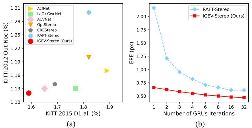
Figure 1: (a) Comparison with state-of-the-art stereo methods[21, 47, 9, 43, 25, 59] on KITTI 2012 and 2015 leaderboards. (b) Performance comparison with RAFT-Stereo[24] on Scene Flow test set as the number of iterations changes.

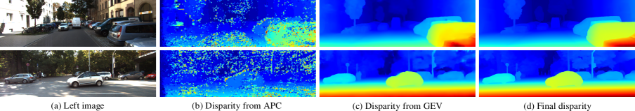
Figure 2: (a) Input images from KITTI 2015. Illustration of (b) disparity regressed from All-pairs Correlations (APC) in RAFT-Stereo[24], (c) disparity regressed from our Geometry Encoding Volume (GEV), (d) our final disparity. The APC lacks non-local geometry knowledge and thus has difficulties tackling local ambiguities in ill-posed region. We take full advantage of cost filtering and iterative optimization: 1) exploiting 3D CNN to filter cost volume and obtain the strong scene representation and the initial disparity with smooth edges, 2) exploiting ConvGRUs to optimize the initial disparity to recover object edges and details.

Recently, iterative optimization-based methods[39, 24, 21, 30, 43] have exhibited attractive performance on both high resolution images and standard benchmarks. Different from existing methods, iterative methods bypass the computationally expensive cost aggregation operations and progressively update the disparity map by repeatedly fetching information from a high-resolution 4D cost volume. Such solution enables the direct usage of high-resolution cost volume and hence is applicable to high-resolution images. For instance, RAFT-Stereo[24] exploits a multi-level Convolutional Gated Recurrent Units (ConvGRUs)[10] to recurrently update the disparity field using local cost values retrieved from all-pairs correlations (APC).

However, without cost aggregation the original cost volume lacks non-local geometry and context information (see Fig. 2 (b)). As a result, existing iterative methods have difficulties tackling local ambiguities in ill-posed regions, such as occlusions, texture-less regions and repetitive structures. Even though, the ConvGRU-based updater can improve the predicted disparities by incorporating context and geometry information from context features and hidden layers, such limitation in the original cost volume greatly limits the effectiveness of each iteration and in turn yield a large amount of ConvGRUs iterations for satisfactory performance.

We claim that cost filtering-based methods and iterative optimization-based methods have complementary advantages and limitations. The former can encode sufficient non-local geometry and context information in the cost volume which is essential for disparity prediction in particular in challenging regions. The latter can avoid high computational and memory cost for 3D cost aggregation, yet are less capable in ill-posed regions based only on all-pairs correlations. To combine complementary advantages of the two methods, we propose Iterative Geometry Encoding Volume (IGEV-Stereo), a new paradigm for stereo matching (see Fig. 3). To address ambiguities caused by ill-posed regions, we compute a Geometry Encoding Volume (GEV) by aggregating and regularizing a cost volume using an extremely lightweight 3D regularization network. Compared to all-pairs correlations of RAFT-Stereo[24], our GEV encodes more geometry and context of the scene after aggregation, shown in Fig. 2 (c). A potential problem of GEV is that it could suffer from over-smoothing at boundaries and tiny details due to the 3D regularization network. To complement local correlations, we combine the GEV and all-pairs correlations to form a Combined Geometry Encoding Volume (CGEV) and input the CGEV into the ConvGRU-based update operator for iterative disparity map optimization.

Our IGEV-Stereo outperforms RAFT-Stereo in terms of both accuracy and efficiency. The performance gains come from two aspects. First, our CGEV provides more comprehensive yet concise information for ConvGRUs to update, yielding more effective optimization in each iteration and in turn could significantly reduce the amount of ConvGRUs iterations. As shown in Fig. 1, our method achieves even smaller EPE (i.e., 0.58) using only 3 ConvGRUs iterations (i.e.,100ms totally for inference) than RAFT-Stereo using 32 ConvGRUs iterations (i.e., EPE of 0.61 and 440ms for inference). Second, our method regresses an initial disparity map from the GEV via $soft\;argmin$ which could provide an accurate starting point for the ConvGRU-based update operator, and in turn yield a fast convergence. In comparison, RAFT-Stereo starts disparity prediction from an initial starting point $\mathbf{d}_{0}$=0, which demands a large number ConvGRUs iterations to achieve an optimized result.

We demonstrate the efficiency and effectiveness of our method on several stereo benchmarks. Our IGEV-Stereo achieves the state-of-the-art EPE of 0.47 on Scene Flow[31] and ranks $1^{st}$ on KITTI 2015[32] and 2012 (Reflective)[15] leaderboards among all the published methods. Regarding the inference speed, our IGEV-Stereo is the fastest among the top 10 methods on KITTI leaderboards. IGEV-Stereo also exhibits better cross-dataset generalization ability than most existing stereo networks. When trained only on synthetic data Scene Flow, our IGEV-Stereo performs very well on real datasets Middlebury[34] and ETH3D[35]. We also extend our IGEV to MVS, i.e. IGEV-MVS, which achieves competitive accuracy on DTU[1].

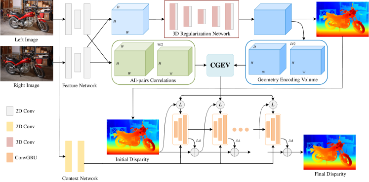
Figure 3: Overview of our proposed IGEV-Stereo. The IGEV-Stereo first builds a Geometry Encoding Volume (GEV) which encodes geometry and context information through 3D CNN, and combines it with All-pairs Correlations (APC) to form a Combined Geometry Encoding Volume (CGEV). Then we regress an initial disparity from GEV and iteratively update it using local cost values retrieved from CGEV through ConvGRUs.

2 Related Work

Cost Filtering-based Methods To improve the representative ability of a cost volume, most existing learning-based stereo methods[5, 33, 23, 49, 45, 46, 12, 52] construct a cost volume using powerful CNN features. However, the cost volume could still suffer from the ambiguity problem in occluded regions, large texture-less/reflective regions and repetitive structures. The 3D convolutional networks have exhibited great potential in regularizing or filtering the cost volume, which can propagate reilable sparse matches to ambiguous and noisy regions. GCNet[20] firstly uses 3D encoder-decoder architecture to regularize a 4D concatenation volume. PSMNet[5] proposes a stacked hourglass 3D CNN in conjunction with intermediate supervision to regularize the concatenation volume. GwcNet[17] and ACVNet[47] propose the group-wise correlation volume and the attention concatenation volume, respectively, to improve the expressiveness of the cost volume and in turn improve the performance in ambiguous regions. GANet[56] designs a semi-global aggregation layer and a local guided aggregation layer to further improve the accuracy. However, the high computational and memory cost of 3D CNNs often prevent these models from being applied to high-resolution cost volumes. To improve efficiency, several cascade methods[36, 16, 48] have been proposed. CFNet[36] and CasStereo[16] build a cost volume pyramid in a coarse-to-fine manner to progressively narrow down the predicted disparity range. Despite their impressive performance, the coarse-to-fine method inevitably involves accumulated errors at coarse resolutions.

Iterative Optimization-based Methods Recently, many iterative methods[39, 24, 41] have been proposed and achieved impressive performance in matching tasks. RAFT-Stereo[24] proposes to recurrently update the disparity field using local cost values retrieved from the all-pairs correlations. However, the all-pair correlations lack non-local information and have difficulties in tackling local ambiguities in ill-posed regions. Our IGEV-Stereo also adopts ConvGRUs as RAFT-Stereo[24] to iteratively update the disparities. Different from RAFT-Stereo[24], we construct a CGEV which encodes non-local geometry and context information, and local matching details to significantly improve the effectiveness of each ConvGRUs iteration. In addition, we provide a better initial disparity map for the ConvGRUs updater to start, yielding a much faster convergence than RAFT-Stereo[24].

3 Method

In this section, we detail the structure of IGEV-Stereo (Fig. 3), which consists of a multi-scale feature extractor, a combined geometry encoding volume, a ConvGRU-based update operator and a spatial upsampling module.

3.1 Feature Extractor

Feature extractor contains two parts: 1) a feature network which extracts multi-scale features for cost volume construction and guiding cost aggregation, and 2) a context network which extracts multi-scale context features for ConvGRUs hidden state initialization and updating.

Feature Network. Given the left and the right images $\mathbf{I}_{l(r)}\in\mathbb{R}^{{3}\times{H}\times{W}}$, we first apply the MobileNetV2 pretrained on ImageNet[11] to scale $\mathbf{I}_{l(r)}$ down to 1/32 of the original size, then use upsampling blocks with skip-connections to recover them up to 1/4 scale, resulting in multi-scale features {$\mathbf{f}_{l,i}(\mathbf{f}_{r,i})\in\mathbb{R}^{{C_{i}}\times{\frac{H}{i}}\times{\frac{W}{i}}}$} ($i$=4, 8, 16, 32 and $C_{i}$ for feature channels). The $\mathbf{f}_{l,4}$ and $\mathbf{f}_{r,4}$ are used to construct the cost volume. And the $\mathbf{f}_{l,i}$ ($i$=4, 8, 16, 32) are used as guidance for 3D regularization network.

Context Network. Following RAFT-Stereo[24], the context network consists of a series of residual blocks and downsampling layers, producing multi-scale context features at 1/4, 1/8 and 1/16 of the input image resolution with 128 channels. The multi-scale context features are used to initialize the hidden state of the ConvGRU-based update operator and also inserted into the ConvGRUs at each iteration.

3.2 Combined Geometry Encoding Volume

Given the left features $\mathbf{f}_{l,4}$ and right features $\mathbf{f}_{r,4}$ extracted from $\mathbf{I}_{l}$ and $\mathbf{I}_{r}$, we construct a group-wise correlation volume[17] that splits features $\mathbf{f}_{l,4}$ ($\mathbf{f}_{r,4}$) into $N_{g}$ ($N_{g}$=8) groups along the channel dimension and compute correlation maps group by group,

$$\mathbf{C}_{corr}(g,d,x,y)=\frac{1}{N_{c}/N_{g}}\langle\mathbf{f}_{l,4}^{g}(x,y),\mathbf{f}_{r,4}^{g}(x-d,y)\rangle,$$ (1)

where $\langle\cdot,\cdot\rangle$ is the inner product, $d$ is the disparity index, $N_{c}$ denotes the number of feature channels. A cost volume $\mathbf{C}_{corr}$ based on only feature correlations lacks the ability to capture global geometric structure. To address this problem, we further process $\mathbf{C}_{corr}$ using a lightweight 3D regularization network $\mathbf{R}$ to obtain the geometry encoding volume $\mathbf{C}_{G}$ as,

$$\mathbf{C}_{G}=\mathbf{R}(\mathbf{C}_{corr})$$ (2)

The 3D regularization network $\mathbf{R}$ is based on a lightweight 3D UNet that consists of three down-sampling blocks and three up-sampling blocks. Each down-sampling block consists of two $3\times 3\times\!3$ 3D convolution. The number of channels of the three down-sampling blocks are 16, 32, 48 respectively. Each up-sampling block consists of a $4\times 4\times 4$ 3D transposed convolution and two $3\times 3\times 3$ 3D convolutions. We follow CoEx[2], which excites the cost volume channels with weights computed from the left features for cost aggregation. For a $\frac{D}{i}\times\frac{H}{i}\times\frac{W}{i}$ cost volume $\mathbf{C}_{i}$ ($i$=4, 8, 16 and 32) in cost aggregation, the guided cost volume excitation is expressed as,

$$\mathbf{C}_{i}^{{}^{\prime}}=\sigma(\mathbf{f}_{l,i})\odot\mathbf{C}_{i},$$ (3)

where $\sigma$ is the sigmoid function, $\odot$ denotes the Hadamard Product. The 3D regularization network, which inserts guided cost volume excitation operation, can effectively infer and propagate scene geometry information, leading to a geometry encoding volume. We also calculate all-pairs correlations between corresponding left and right features to obtain local feature correlations.

To increase the receptive field, we pool the disparity dimension using 1D average pooling with a kernel size of 2 and a stride of 2 to form a two-level $\mathbf{C}_{G}$ pyramid and all-pairs correlation volume $\mathbf{C}_{A}$ pyramid. Then we combine the $\mathbf{C}_{G}$ pyramid and $\mathbf{C}_{A}$ pyramid to form a combined geometry encoding volume.

3.3 ConvGRU-based Update Operator

We apply $soft\;argmin$ to regress an initial starting disparity $\mathbf{d}_{0}$ from the geometry encoding volume $\mathbf{C}_{G}$ according to Equ. 4,

$$\mathbf{d}_{0}=\sum\limits_{d=0}^{D-1}d\times Softmax(\mathbf{C}_{G}(d)),$$ (4)

where $d$ is a predetermined set of disparity indices at 1/4 resolution. Then from $\mathbf{d}_{0}$, we use three levels of ConvGRUs to iteratively update the disparity (shown in Fig. 3). This setup facilitates a fast convergence of iterative disparity optimization. The hidden state of three levels of ConvGRUs are initialized from the multi-scale context features.

For each iteration, we use the current disparity $\mathbf{d}_{k}$ to index from the combined geometry encoding volume via linear interpolation, producing a set of geometry features $\mathbf{G}_{f}$. The $\mathbf{G}_{f}$ is computed by,

$$\mathbf{G}_{f}=\sum\limits_{i=-r}^{r}\text{Concat}\{\mathbf{C}_{G}(\mathbf{d}_{k}\!+\!i),\mathbf{C}_{A}(\mathbf{d}_{k}\!+\!i),$$ (5)

$$\mathbf{C}_{G}^{p}({\mathbf{d}_{k}}/2\!+\!i),\mathbf{C}_{A}^{p}({\mathbf{d}_{k}}/2\!+\!i)\},$$

where $\mathbf{d}_{k}$ is the current disparity, $r$ is indexing radius, and $p$ denotes the pooling operation. These geometry features and current disparity prediction $\mathbf{d}_{k}$ are passed through two encoder layers and then concatenated with $\mathbf{d}_{k}$ to form $x_{k}$. Then we use ConvGRUs to update the hidden state $h_{k-1}$ as RAFT-Stereo[24],

$$x_{k}= \;[\text{Encoder}_{g}(\mathbf{G}_{f}),\text{Encoder}_{d}(\mathbf{d}_{k}),\mathbf{d}_{k}]$$ (6)

$$z_{k}= \;\sigma(\text{Conv}([h_{k-1},x_{k}],W_{z})+c_{k}),$$

$$r_{k}= \;\sigma(\text{Conv}([h_{k-1},x_{k}],W_{r})+c_{r}),$$

$$\tilde{h}_{k}= \,\tanh(\text{Conv}([r_{k}\odot h_{k-1},x_{k}],W_{h})+c_{h}),$$

$$h_{k}= \;(1-z_{k})\odot h_{k-1}+z_{k}\odot\tilde{h}_{k},$$

where $c_{k}$, $c_{r}$, $c_{h}$ are context features generated from the context network. The number of channels in the hidden states of ConvGRUs is 128, and the number of channels of the context feature is also 128. The $\text{Encoder}_{g}$ and $\text{Encoder}_{d}$ consist of two convolutional layers respectively. Based on the hidden state $h_{k}$, we decode a residual disparity $\triangle\mathbf{d}_{k}$ through two convolutional layers, then we update the current disparity,

$$\mathbf{d}_{k+1}= \;\mathbf{d}_{k}+\triangle\mathbf{d}_{k}$$ (7)

3.4 Spatial Upsampling

We output a full resolution disparity map by the weighted combination of the predicted disparity $\mathbf{d}_{k}$ at 1/4 resolution. Different from RAFT-Stereo[24] which predicts weights from the hidden state ${h_{k}}$ at 1/4 resolution, we utilize the higher resolution context features to obtain the weights. We convolve the hidden state to generate features and then upsample them to 1/2 resolution. The upsampled features are concatenated with $\mathbf{f}_{l,2}$ from left image to produce weights $\mathbf{W}\in\mathbb{R}^{H\times{W}\times 9}$. We output the full resolution disparities by the weighted combination of their coarse resolution neighbors.

3.5 Loss Function

We calculate the smooth L1 loss[5] on initial disparity $\mathbf{d}_{0}$ regressed from GEV:

$$\mathcal{L}_{init}=Smooth_{L_{1}}(\mathbf{d}_{0}-\mathbf{d}_{gt})$$ (8)

where $\mathbf{d}_{gt}$ represents the ground truth disparity. We calculate the L1 loss on all predicted disparities $\{\mathbf{d}_{i}\}_{i=1}^{N}$. We follow [24] to exponentially increase the weights, and the total loss is defined as:

$$\mathcal{L}_{stereo}=\mathcal{L}_{init}+\sum_{i=1}^{N}\gamma^{N-i}||\mathbf{d}_{i}-\mathbf{d}_{gt}||_{1},$$ (9)

where $\gamma=0.9$, and ${\mathbf{d}}_{gt}$ represent ground truth.

Model	All-pairs correlations	GEV	Init disp from GEV	Supervise for GEV	EPE (px)	>3px (%)	Time (s)	Params. (M)
Baseline	✓				0.56	2.85	0.36	12.02
G		✓			0.51	2.68	0.37	12.60
G+I		✓	✓		0.50	2.62	0.37	12.60
G+I+S		✓	✓	✓	0.48	2.51	0.37	12.60
Full model (IGEV-Stereo)	✓	✓	✓	✓	0.47	2.47	0.37	12.60

Table 1: Ablation study of proposed networks on the Scene Flow test set. GEV denotes Geometry Encoding Volume. The baseline is RAFT-Stereo using MobileNetV2 100 as backbone. The time is the inference time for 960$\times$540 inputs.

4 Experiment

Scene Flow[31] is a synthetic dataset containing 35, 454 training pairs and 4,370 testing pairs with dense disparity maps. We use the Finalpass of Scene Flow, since it is more like real-world images than the Cleanpass, which contains more motion blur and defocus.

KITTI 2012[15] and KITTI 2015[32] are datasets for real-world driving scenes. KITTI 2012 contains 194 training pairs and 195 testing pairs, and KITTI 2015 contains 200 training pairs and 200 testing pairs. Both datasets provide sparse ground-truth disparities obtained with LIDAR.

Middlebury 2014[34] is an indoor dataset, which provides 15 training pairs and 15 testing pairs, where some samples are under inconsistent illumination or color conditions. All of the images are available in three different resolutions. ETH3D[35] is a gray-scale dataset with 27 training pairs and 20 testing pairs. We use the training pairs of Middlebury 2014 and ETH3D to evaluate cross-domain generalization performance.

4.1 Implementation Details

We implement our IGEV-Stereo with PyTorch and perform our experiments using NVIDIA RTX 3090 GPUs. For all training, we use the AdamW[28] optimizer and clip gradients to the range [-1, 1]. On Scene Flow, we train IGEV-Stereo for 200k steps with a batch size of 8. On KITTI, we finetune the pre-trained Scene Flow model on the mixed KITTI 2012 and KITTI 2015 training image pairs for 50k steps. We randomly crop images to $320\times 736$ and use the same data augmentation as [24] for training. The indexing radius is set to 4. For all experiments, we use a one-cycle learning rate schedule with a learning rate of 0.0002, and we use 22 update iterations during training.

Model	Number of Iterations
	1	2	3	4	8	32
RAFT-Stereo[24]	2.16	1.21	0.95	0.82	0.66	0.61
G	0.98	0.73	0.66	0.62	0.54	0.51
G+I+S	0.67	0.63	0.59	0.56	0.51	0.48
Full model	0.66	0.62	0.58	0.55	0.50	0.47

Table 2: Ablation study for number of iterations.

Experiment	Variations	Scene Flow	Params.(M)
GEV Reso.	1/8	0.49	12.71
	1/4	0.47	12.60
Backbone	MobileNetV2 100	0.47	12.60
	MobileNetV2 120d	0.46	15.05
	ConvNeXt-B	0.45	18.04

Table 3: Ablation experiments. Settings used in our final model are underlined.

Method	PSMNet[5]	GwcNet[17]	GANet[56]	CSPN[8]	LEAStereo[9]	ACVNet[47]	IGEV-Stereo (Ours)
EPE (px)	1.09	0.76	0.84	0.78	0.78	0.48	0.47

Table 4: Quantitative evaluation on Scene Flow test set. Bold: Best.

Method	KITTI 2012[15]						KITTI 2015[32]			Run-time (s)
	2-noc	2-all	3-noc	3-all	EPE noc	EPE all	D1-bg	D1-fg	D1-all
PSMNet[5]	2.44	3.01	1.49	1.89	0.5	0.6	1.86	4.62	2.32	0.41
GwcNet[17]	2.16	2.71	1.32	1.70	0.5	0.5	1.74	3.93	2.11	0.32
GANet-deep[56]	1.89	2.50	1.19	1.60	0.4	0.5	1.48	3.46	1.81	1.80
AcfNet[59]	1.83	2.35	1.17	1.54	0.5	0.5	1.51	3.80	1.89	0.48
HITNet[38]	2.00	2.65	1.41	1.89	0.4	0.5	1.74	3.20	1.98	0.02
EdgeStereo-V2[37]	2.32	2.88	1.46	1.83	0.4	0.5	1.84	3.30	2.08	0.32
CSPN[36]	1.79	2.27	1.19	1.53	-	-	1.51	2.88	1.74	1.00
LEAStereo[9]	1.90	2.39	1.13	1.45	0.5	0.5	1.40	2.91	1.65	0.30
ACVNet[47]	1.83	2.35	1.13	1.47	0.4	0.5	1.37	3.07	1.65	0.20
CREStereo[21]	1.72	2.18	1.14	1.46	0.4	0.5	1.45	2.86	1.69	0.41
RAFT-Stereo[24]	1.92	2.42	1.30	1.66	0.4	0.5	1.58	3.05	1.82	0.38
IGEV-Stereo (Ours)	1.71	2.17	1.12	1.44	0.4	0.4	1.38	2.67	1.59	0.18

Table 5: Quantitative evaluation on KITTI 2012 [15] and KITTI 2015 [32]. The IGEV-Stereo runs 16 updates at inference. Bold: Best.

Method	Iters	2-noc	2-all	3-noc	3-all
RAFT-Stereo[24]	8	9.98	11.95	6.64	8.04
	16	8.83	10.35	5.76	6.84
	32	8.41	9.87	5.40	6.48
IGEV-Stereo	8	8.30	9.82	4.88	5.87
	16	7.57	8.80	4.35	5.00
	32	7.29	8.48	4.11	4.76

Table 6: Evaluation in the reflective regions (ill-posed regions) of KITTI 2012 benchmark. Iters denotes iteration number.

4.2 Ablation Study

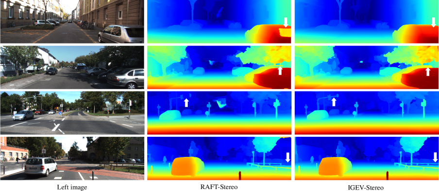
Figure 4: Qualitative results on the test set of KITTI. The first two columns show results on KITTI 2012, and the last two columns show results on KITTI 2015. Our IGEV-Stereo performs very well in textureless and detailed regions.

Effectiveness of CGEV. We explore the best settings for the combined geometry encoding volume (CGEV) and exam its effectiveness. For all models in these experiments, we perform 32 iterations of ConvGRUs updating at inference. We take RAFT-Stereo as our baseline, and replace its original backbone with MobileNetV2 100. As shown in Tab. 1, the proposed GEV can significantly improve the prediction accuracy. Compared with all-pairs correlations in RAFT-Stereo[24], the GEV can provide non-local information and scene prior knowledge, thus the prediction error decreases evidently. RAFT-Stereo uses a starting disparity initialized to zero, thus increasing the number of iterations to reach optimal results. In contrast, we apply the $soft\;argmin$ to regress an initial starting disparity from GEV, which speeds up the convergence and slightly reduces the prediction error. To further explicitly constrain GEV during training, we use ground truth disparity to supervise GEV, deriving accurate GEV and starting disparity. When processed by the 3D regularization network, the GEV suffers from the over-smoothing problem at boundaries and tiny details. To complement local correlations, we combine the GEV and all-pairs correlations to form a combined geometry encoding volume (CGEV). The proposed CGEV, denoted as IGEV-Stereo, achieves the best performance.

Number of Iterations. Our IGEV-Stereo achieves excellent performance even when the number of iterations is reduced. As shown in Tab. 2, we report the EPE of our models and RAFT-Stereo on Scene Flow. Compared with all-pairs correlations in RAFT-Stereo, our GEV can provide more accurate geometry and context information. Thus when the number of iterations is reduced to 1, 2, 3 or 4, our IGEV-Stereo (G) can outperform RAFT-Stereo with the same number of iterations by a large margin, such as surpassing RAFT-Stereo by 54.63% at 1 iteration. When regressing an initial disparity $\mathbf{d}_{0}$ from GEV and supervising it, we obtain an accurate initial disparity to update and thus the prediction error can decrease evidently. Finally, when changing the number of iterations, our full model, denoted as IGEV-Stereo, achieves the best performance, which surpasses RAFT-Stereo by 69.44% at 1 iteration. From Tab. 2, we can observe that our IGEV-Stereo achieves the state-of-the-art performance even with few iterations, enabling the users to trade off time efficiency and performance according to their needs.

Configuration Exploration. Tab. 3 shows results of different configurations. Even constructing a 1/8 resolution GEV that takes only 5ms extra, our method still achieves state-of-the-art performance with an EPE of 0.49 on Scene Flow. When using the backbone with more parameters, i.e. MobileNetV2 120d and ConvNeXt-B[27], the performance can be improved.

4.3 Comparisons with State-of-the-art

We compare IGEV-Stereo with the published state-of-the-art methods on Scene Flow, KITTI 2012 and 2015. On Scene Flow test set, we achieve a new SOTA EPE of 0.47, which surpasses CSPN[8] and LEAStereo[9] by 39.74%. Compared to the classical PSMNet[5], our IGEV-Stereo not only achieves $2\times$ better accuracy, but is also faster than it. Quantitative comparisons are shown in Tab. 4. We evaluate our IGEV-Stereo on the test set of KITTI 2012 and 2015, and the results are submitted to the online KITTI leaderboard. As shown in Tab. 5, we achieve the best performance among the published methods for almost all metrics on KITTI 2012 and 2015. At the time of writing, our IGEV-Stereo ranks $1^{st}$ on the KITTI 2015 leaderboard compared with over 280 methods. On KITTI 2012, our IGEV-Stereo outperforms LEAStereo[9] and RAFT-Stereo[24] by 10.00% and 10.93% on Out-Noc under 2 pixels error threshold, respectively. On KITTI 2015, our IGEV-Stereo surpasses CREStereo[21] and RAFT-Stereo[24] by 5.92% and 12.64% on D1-all metric, respectively. Specially, compared with other iterative methods such as CREStereo[21] and RAFT-Stereo[24], our IGEV-Stereo not only outperforms them, but is also $2\times$ faster. Fig. 4 shows qualitative results on KITTI 2012 and 2015. Our IGEV-Stereo performs very well in reflective and detailed regions.

We evaluate the performance of IGEV-Stereo and RAFT-Stereo in the ill-posed regions, shown in Tab. 6. RAFT-Stereo lacks non-local knowledge and thus has difficulties tackling local ambiguities in ill-posed regions. Our IGEV-Stereo can well overcome these problems. IGEV-Stereo ranks $1^{st}$ on KITTI 2012 leaderboard for reflective regions, which outperforms RAFT-Stereo by a large margin. Specially, our method performs better using only 8 iterations than RAFT-Stereo using 32 iterations in the reflective regions.

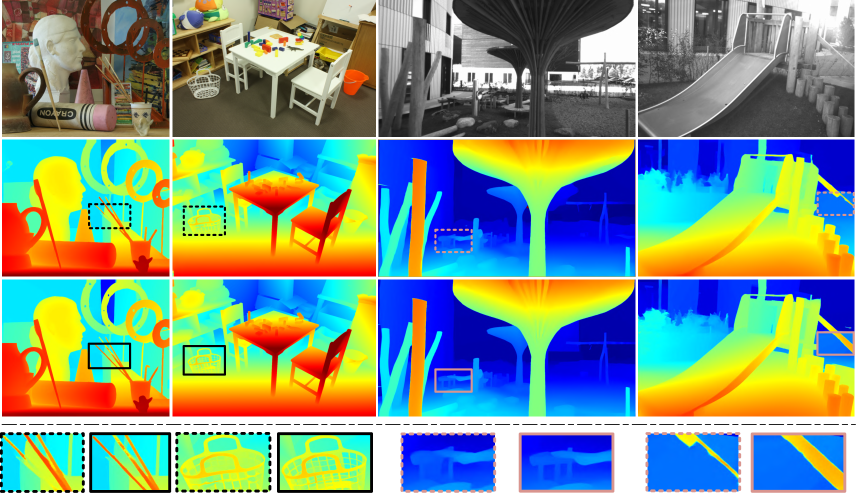
Figure 5: Generalization results on Middlebury 2014 and ETH3D. The second and the third rows are the results of RAFT-Stereo[24] and our IGEV-Stereo, respectively. Our IGEV-Stereo exhibits better details for fine-structured objects.

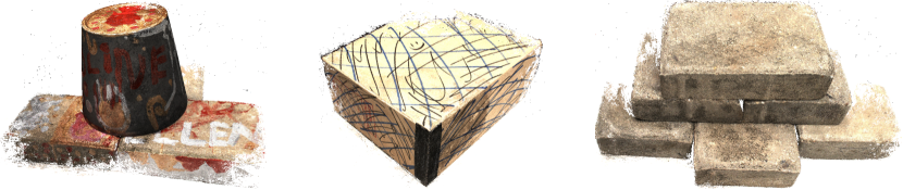
Figure 6: Visualization of results on DTU [1] test set.

Model	Middlebury		ETH3D
	half	quarter
CostFilter[19]	40.5	17.6	31.1
PatchMatch[3]	38.6	16.1	24.1
SGM[18]	25.2	10.7	12.9
PSMNet[5]	15.8	9.8	10.2
GANet[56]	13.5	8.5	6.5
DSMNet[57]	13.8	8.1	6.2
STTR[22]	15.5	9.7	17.2
CFNet[36]	15.3	9.8	5.8
FC-GANet[58]	10.2	7.8	5.8
Graft-GANet[26]	9.8	-	6.2
RAFT-Stereo[24]	8.7	7.3	3.2
IGEV-Stereo (Ours)	7.1	6.2	3.6

Table 7: Synthetic to real generalization experiments. All models are trained on Scene Flow. The 2-pixel error rate is used for Middlebury 2014, and 1-pixel error rate for ETH3D.

4.4 Zero-shot Generalization

Since large real-world datasets for training are difficult to obtain, the generalization ability of stereo models is crucial. We evaluate the generalization performance of IGEV-Stereo from synthetic datasets to unseen real-world scenes. In this evaluation, we train our IGEV-Stereo on Scene Flow using data augmentation, and directly test it on the Middlebury 2014 and ETH3D training sets. As shown in Tab. 7, our IGEV-Stereo achieves state-of-the-art performance in the same zero-shot setting. Fig. 5 shows a visual comparison with RAFT-Stereo, our method is more robust for textureless and detailed regions.

4.5 Extension to MVS

We extend our IGEV to multi-view stereo (MVS), i.e. IGEV-MVS. We evaluate our IGEV-MVS on the DTU[1] benchmark. DTU is an indoor multi-view stereo dataset with 124 different scenes and 7 different lighting conditions. Following the IterMVS[41], the DTU is split into training, validation and testing set. We use an image resolution of $640\times 512$ and the number of input images is N=5 for training. We train IGEV-MVS on DTU for 32 epochs. For evaluation, image size, number of views and number of iterations are set to $1600\times 1152$, 5 and 32 respectively. Compared with IGEV-Stereo, IGEV-MVS removes context network that means that ConvGRUs does not access context stream. As shown in Tab. 8, our IGEV-MVS achieves the best overall score, which is an average of completeness and accuracy. Especially, compared with PatchmatchNet[42] and IterMVS[41], our IGEV-MVS achieves 8.0% and 10.7% relative improvements on the overall quality.

Method	Acc.(mm)$\downarrow$	Comp.(mm)$\downarrow$	Overall(mm)$\downarrow$
Camp[4]	0.835	0.554	0.695
Furu[13]	0.613	0.941	0.777
Tola[40]	0.342	1.190	0.766
Gipuma[14]	0.283	0.873	0.578
MVSNet[53]	0.396	0.527	0.462
R-MVSNet[54]	0.383	0.452	0.417
P-MVSNet[29]	0.406	0.434	0.420
Point-MVSNet[6]	0.342	0.411	0.376
Fast-MVSNet[55]	0.336	0.403	0.370
AA-RMVSNet[44]	0.376	0.339	0.357
CasMVSNet[16]	0.325	0.385	0.355
UCS-Net[7]	0.338	0.349	0.344
CVP-MVSNet[50]	0.296	0.406	0.351
MVS2D[51]	0.394	0.290	0.342
PatchmatchNet[42]	0.427	0.277	0.352
IterMVS[41]	0.373	0.354	0.363
CER-MVS[30]	0.359	0.305	0.332
IGEV-MVS (Ours)	0.331	0.316	0.324

Table 8: Quantitative evaluation on DTU. Methods are separated into two categories (from top to bottom): traditional and trained on DTU.

5 Conclusion and Future Work

We propose Iterative Geometry Encoding Volume (IGEV), a new deep network architecture for stereo matching and multi-view stereo (MVS). The IGEV builds a combined geometry encoding volume that encodes geometry and context information as well as local matching details, and iteratively indexes it to update the disparity map. Our IGEV-Stereo ranks $1^{st}$ on KITTI 2015 leaderboard among all the published methods and achieves state-of-the-art cross-dataset generalization ability. Our IGEV-MVS also achieves competitive performance on DTU benchmark.

We use a lightweight 3D CNN to filter the cost volume and obtain GEV. However, when dealing with high-resolution images that exhibit a large disparity range, using a 3D CNN to process the resulting large-size cost volume can still lead to high computational and memory costs. Future work includes designing a more lightweight regularization network. In addition, we will also explore the utilization of cascaded cost volumes to make our method applicable to high-resolution images.

Acknowledgement. We thank all the reviewers for their valuable comments. This research is supported by National Natural Science Foundation of China (62122029, 62061160490) and Applied Fundamental Research of Wuhan (2020010601012167).

References

- [1] Henrik Aanæs, Rasmus Ramsbøl Jensen, George Vogiatzis, Engin Tola, and Anders Bjorholm Dahl. Large-scale data for multiple-view stereopsis. IJCV, 120(2):153–168, 2016.
- [2] Antyanta Bangunharcana, Jae Won Cho, Seokju Lee, In So Kweon, Kyung-Soo Kim, and Soohyun Kim. Correlate-and-excite: Real-time stereo matching via guided cost volume excitation. In IROS, pages 3542–3548. IEEE, 2021.
- [3] Michael Bleyer, Christoph Rhemann, and Carsten Rother. Patchmatch stereo-stereo matching with slanted support windows. In BMVC, volume 11, pages 1–11, 2011.
- [4] Neill DF Campbell, George Vogiatzis, Carlos Hernández, and Roberto Cipolla. Using multiple hypotheses to improve depth-maps for multi-view stereo. In ECCV, pages 766–779. Springer, 2008.
- [5] Jia-Ren Chang and Yong-Sheng Chen. Pyramid stereo matching network. In CVPR, pages 5410–5418, 2018.
- [6] Rui Chen, Songfang Han, Jing Xu, and Hao Su. Point-based multi-view stereo network. In ICCV, pages 1538–1547, 2019.
- [7] Shuo Cheng, Zexiang Xu, Shilin Zhu, Zhuwen Li, Li Erran Li, Ravi Ramamoorthi, and Hao Su. Deep stereo using adaptive thin volume representation with uncertainty awareness. In CVPR, pages 2524–2534, 2020.
- [8] Xinjing Cheng, Peng Wang, and Ruigang Yang. Learning depth with convolutional spatial propagation network. IEEE TPAMI, 42(10):2361–2379, 2019.
- [9] Xuelian Cheng, Yiran Zhong, Mehrtash Harandi, Yuchao Dai, Xiaojun Chang, Hongdong Li, Tom Drummond, and Zongyuan Ge. Hierarchical neural architecture search for deep stereo matching. NeurIPS, 33:22158–22169, 2020.
- [10] Kyunghyun Cho, Bart Van Merriënboer, Caglar Gulcehre, Dzmitry Bahdanau, Fethi Bougares, Holger Schwenk, and Yoshua Bengio. Learning phrase representations using rnn encoder-decoder for statistical machine translation. arXiv preprint arXiv:1406.1078, 2014.
- [11] Jia Deng, Wei Dong, Richard Socher, Li-Jia Li, Kai Li, and Li Fei-Fei. Imagenet: A large-scale hierarchical image database. In CVPR, pages 248–255. Ieee, 2009.
- [12] Shivam Duggal, Shenlong Wang, Wei-Chiu Ma, Rui Hu, and Raquel Urtasun. Deeppruner: Learning efficient stereo matching via differentiable patchmatch. In ICCV, pages 4384–4393, 2019.
- [13] Yasutaka Furukawa and Jean Ponce. Accurate, dense, and robust multiview stereopsis. IEEE TPAMI, 32(8):1362–1376, 2009.
- [14] Silvano Galliani, Katrin Lasinger, and Konrad Schindler. Massively parallel multiview stereopsis by surface normal diffusion. In ICCV, pages 873–881, 2015.
- [15] Andreas Geiger, Philip Lenz, and Raquel Urtasun. Are we ready for autonomous driving? the kitti vision benchmark suite. In CVPR, pages 3354–3361. IEEE, 2012.
- [16] Xiaodong Gu, Zhiwen Fan, Siyu Zhu, Zuozhuo Dai, Feitong Tan, and Ping Tan. Cascade cost volume for high-resolution multi-view stereo and stereo matching. In CVPR, pages 2495–2504, 2020.
- [17] Xiaoyang Guo, Kai Yang, Wukui Yang, Xiaogang Wang, and Hongsheng Li. Group-wise correlation stereo network. In CVPR, pages 3273–3282, 2019.
- [18] Heiko Hirschmuller. Stereo processing by semiglobal matching and mutual information. IEEE TPAMI, 30(2):328–341, 2007.
- [19] Asmaa Hosni, Christoph Rhemann, Michael Bleyer, Carsten Rother, and Margrit Gelautz. Fast cost-volume filtering for visual correspondence and beyond. IEEE TPAMI, 35(2):504–511, 2012.
- [20] Alex Kendall, Hayk Martirosyan, Saumitro Dasgupta, Peter Henry, Ryan Kennedy, Abraham Bachrach, and Adam Bry. End-to-end learning of geometry and context for deep stereo regression. In ICCV, pages 66–75, 2017.
- [21] Jiankun Li, Peisen Wang, Pengfei Xiong, Tao Cai, Ziwei Yan, Lei Yang, Jiangyu Liu, Haoqiang Fan, and Shuaicheng Liu. Practical stereo matching via cascaded recurrent network with adaptive correlation. In CVPR, pages 16263–16272, 2022.
- [22] Zhaoshuo Li, Xingtong Liu, Nathan Drenkow, Andy Ding, Francis X Creighton, Russell H Taylor, and Mathias Unberath. Revisiting stereo depth estimation from a sequence-to-sequence perspective with transformers. In ICCV, pages 6197–6206, 2021.
- [23] Zhengfa Liang, Yulan Guo, Yiliu Feng, Wei Chen, Linbo Qiao, Li Zhou, Jianfeng Zhang, and Hengzhu Liu. Stereo matching using multi-level cost volume and multi-scale feature constancy. IEEE TPAMI, 2019.
- [24] Lahav Lipson, Zachary Teed, and Jia Deng. Raft-stereo: Multilevel recurrent field transforms for stereo matching. In 3DV, pages 218–227. IEEE, 2021.
- [25] Biyang Liu, Huimin Yu, and Yangqi Long. Local similarity pattern and cost self-reassembling for deep stereo matching networks. In AAAI, volume 36, pages 1647–1655, 2022.
- [26] Biyang Liu, Huimin Yu, and Guodong Qi. Graftnet: Towards domain generalized stereo matching with a broad-spectrum and task-oriented feature. In CVPR, pages 13012–13021, 2022.
- [27] Zhuang Liu, Hanzi Mao, Chao-Yuan Wu, Christoph Feichtenhofer, Trevor Darrell, and Saining Xie. A convnet for the 2020s. In CVPR, pages 11976–11986, 2022.
- [28] Ilya Loshchilov and Frank Hutter. Decoupled weight decay regularization. arXiv preprint arXiv:1711.05101, 2017.
- [29] Keyang Luo, Tao Guan, Lili Ju, Haipeng Huang, and Yawei Luo. P-mvsnet: Learning patch-wise matching confidence aggregation for multi-view stereo. In ICCV, pages 10452–10461, 2019.
- [30] Zeyu Ma, Zachary Teed, and Jia Deng. Multiview stereo with cascaded epipolar raft. arXiv preprint arXiv:2205.04502, 2022.
- [31] Nikolaus Mayer, Eddy Ilg, Philip Hausser, Philipp Fischer, Daniel Cremers, Alexey Dosovitskiy, and Thomas Brox. A large dataset to train convolutional networks for disparity, optical flow, and scene flow estimation. In CVPR, pages 4040–4048, 2016.
- [32] Moritz Menze and Andreas Geiger. Object scene flow for autonomous vehicles. In CVPR, pages 3061–3070, 2015.
- [33] Guang-Yu Nie, Ming-Ming Cheng, Yun Liu, Zhengfa Liang, Deng-Ping Fan, Yue Liu, and Yongtian Wang. Multi-level context ultra-aggregation for stereo matching. In CVPR, pages 3283–3291, 2019.
- [34] Daniel Scharstein, Heiko Hirschmüller, York Kitajima, Greg Krathwohl, Nera Nešić, Xi Wang, and Porter Westling. High-resolution stereo datasets with subpixel-accurate ground truth. In GCPR, pages 31–42. Springer, 2014.
- [35] Thomas Schops, Johannes L Schonberger, Silvano Galliani, Torsten Sattler, Konrad Schindler, Marc Pollefeys, and Andreas Geiger. A multi-view stereo benchmark with high-resolution images and multi-camera videos. In CVPR, pages 3260–3269, 2017.
- [36] Zhelun Shen, Yuchao Dai, and Zhibo Rao. Cfnet: Cascade and fused cost volume for robust stereo matching. In CVPR, pages 13906–13915, 2021.
- [37] Xiao Song, Xu Zhao, Liangji Fang, Hanwen Hu, and Yizhou Yu. Edgestereo: An effective multi-task learning network for stereo matching and edge detection. IJCV, 128(4):910–930, 2020.
- [38] Vladimir Tankovich, Christian Hane, Yinda Zhang, Adarsh Kowdle, Sean Fanello, and Sofien Bouaziz. Hitnet: Hierarchical iterative tile refinement network for real-time stereo matching. In CVPR, pages 14362–14372, 2021.
- [39] Zachary Teed and Jia Deng. Raft: Recurrent all-pairs field transforms for optical flow. In ECCV, pages 402–419. Springer, 2020.
- [40] Engin Tola, Christoph Strecha, and Pascal Fua. Efficient large-scale multi-view stereo for ultra high-resolution image sets. Machine Vision and Applications, 23(5):903–920, 2012.
- [41] Fangjinhua Wang, Silvano Galliani, Christoph Vogel, and Marc Pollefeys. Itermvs: Iterative probability estimation for efficient multi-view stereo. In CVPR, pages 8606–8615, 2022.
- [42] Fangjinhua Wang, Silvano Galliani, Christoph Vogel, Pablo Speciale, and Marc Pollefeys. Patchmatchnet: Learned multi-view patchmatch stereo. In CVPR, pages 14194–14203, 2021.
- [43] Hengli Wang, Rui Fan, Peide Cai, and Ming Liu. Pvstereo: Pyramid voting module for end-to-end self-supervised stereo matching. IEEE Robotics and Automation Letters, 6(3):4353–4360, 2021.
- [44] Zizhuang Wei, Qingtian Zhu, Chen Min, Yisong Chen, and Guoping Wang. Aa-rmvsnet: Adaptive aggregation recurrent multi-view stereo network. In ICCV, pages 6187–6196, 2021.
- [45] Zhenyao Wu, Xinyi Wu, Xiaoping Zhang, Song Wang, and Lili Ju. Semantic stereo matching with pyramid cost volumes. In ICCV, pages 7484–7493, 2019.
- [46] Bin Xu, Yuhua Xu, Xiaoli Yang, Wei Jia, and Yulan Guo. Bilateral grid learning for stereo matching networks. In CVPR, pages 12497–12506, 2021.
- [47] Gangwei Xu, Junda Cheng, Peng Guo, and Xin Yang. Attention concatenation volume for accurate and efficient stereo matching. In CVPR, pages 12981–12990, 2022.
- [48] Gangwei Xu, Yun Wang, Junda Cheng, Jinhui Tang, and Xin Yang. Accurate and efficient stereo matching via attention concatenation volume. arXiv preprint arXiv:2209.12699, 2022.
- [49] Guorun Yang, Hengshuang Zhao, Jianping Shi, Zhidong Deng, and Jiaya Jia. Segstereo: Exploiting semantic information for disparity estimation. In ECCV, pages 636–651, 2018.
- [50] Jiayu Yang, Wei Mao, Jose M Alvarez, and Miaomiao Liu. Cost volume pyramid based depth inference for multi-view stereo. In CVPR, pages 4877–4886, 2020.
- [51] Zhenpei Yang, Zhile Ren, Qi Shan, and Qixing Huang. Mvs2d: Efficient multi-view stereo via attention-driven 2d convolutions. In CVPR, pages 8574–8584, 2022.
- [52] Chengtang Yao, Yunde Jia, Huijun Di, Pengxiang Li, and Yuwei Wu. A decomposition model for stereo matching. In CVPR, pages 6091–6100, 2021.
- [53] Yao Yao, Zixin Luo, Shiwei Li, Tian Fang, and Long Quan. Mvsnet: Depth inference for unstructured multi-view stereo. In ECCV, pages 767–783, 2018.
- [54] Yao Yao, Zixin Luo, Shiwei Li, Tianwei Shen, Tian Fang, and Long Quan. Recurrent mvsnet for high-resolution multi-view stereo depth inference. In CVPR, pages 5525–5534, 2019.
- [55] Zehao Yu and Shenghua Gao. Fast-mvsnet: Sparse-to-dense multi-view stereo with learned propagation and gauss-newton refinement. In CVPR, pages 1949–1958, 2020.
- [56] Feihu Zhang, Victor Prisacariu, Ruigang Yang, and Philip HS Torr. Ga-net: Guided aggregation net for end-to-end stereo matching. In CVPR, pages 185–194, 2019.
- [57] Feihu Zhang, Xiaojuan Qi, Ruigang Yang, Victor Prisacariu, Benjamin Wah, and Philip Torr. Domain-invariant stereo matching networks. In ECCV, pages 420–439. Springer, 2020.
- [58] Jiawei Zhang, Xiang Wang, Xiao Bai, Chen Wang, Lei Huang, Yimin Chen, Lin Gu, Jun Zhou, Tatsuya Harada, and Edwin R Hancock. Revisiting domain generalized stereo matching networks from a feature consistency perspective. In CVPR, pages 13001–13011, 2022.
- [59] Youmin Zhang, Yimin Chen, Xiao Bai, Suihanjin Yu, Kun Yu, Zhiwei Li, and Kuiyuan Yang. Adaptive unimodal cost volume filtering for deep stereo matching. In AAAI, volume 34, pages 12926–12934, 2020.