Correlation between upstreamness and downstreamness in random global value chains

Abstract

This paper is concerned with upstreamness and downstreamness of industries and countries in global value chains. Upstreamness and downstreamness measure respectively the average distance of an industrial sector from final consumption and from primary inputs, and they are computed from based on the most used global Input-Output tables databases, e.g., the World Input-Output Database (WIOD). Recently, Antràs and Chor reported a puzzling and counter-intuitive finding in data from the period 1995-2011, namely that (at country level) upstreamness appears to be positively correlated with downstreamness, with a correlation slope close to $+1$. This effect is stable over time and across countries, and it has been confirmed and validated by later analyses. We analyze a simple model of random Input/Output tables, and we show that, under minimal and realistic structural assumptions, there is a positive correlation between upstreamness and downstreamness of the same industrial sector, with correlation slope equal to $+1$. This effect is robust against changes in the randomness of the entries of the I/O table and different aggregation protocols. Our results suggest that the empirically observed puzzling correlation may rather be a necessary consequence of the few structural constraints (positive entries, and sub-stochasticity) that Input/Output tables and their surrogates must meet.

[inst1]organization=Dept. of Computer Science, University College London,addressline=66-72 Gower Street, city=London, postcode=WC1E 6EA, country=United Kingdom

[inst2]organization=Centre for Financial Technology, Imperial College Business School,addressline=South Kensington, city=London, postcode=SW7 2AZ, country=United Kingdom

[inst3]organization=Systemic Risk Centre, London School of Economics and Political Sciences,addressline=, city=London, postcode=WC2A 2AE, country=United Kingdom

[inst4]organization=London Mathematical Laboratory,addressline=8 Margravine Gardens, city=London, postcode=WC 8RH, country=United Kingdom

[inst5]organization=Theoretical Division (T4), Condensed Matter $\&$ Complex Systems, Los Alamos National Laboratory,city=Los Alamos, postcode=87545, state=New Mexico, country=U.S.A.

[inst6]organization=Dept. of Mathematics, King’s College London,addressline=Strand, city=London, postcode=WC2R 2LS, country=United Kingdom

1 Introduction

The structure of national and international trade flows has undergone a dramatic transformation in the past decades. Understanding how global value chains shape the exchange of goods and money at different scales (from industrial sectors to countries) has become of central importance. Researches on these issues usually rely on Input-Output analysis – the field pioneered by V. Leontief [1, 2]. This level of analysis is facilitated by the increasing availability and development of detailed Input/Output (I-O) tables for each country [3, 4].

To characterize the complexity of global value chains, metrics have been devised that take such empirical I-O tables as starting point. In particular, Antràs and Chor [5], Miller and Temurshoev [6] and Fally [7] introduced the notions of upstreamness and downstreamness to quantify the position of each economic sectors (and countries as a whole) with respect to final consumption, and raw materials, respectively (see Section 2 for details).

In a recent paper that has attracted much attention, Antràs and Chor [8] reported empirical observations of a puzzling correlation existing between the upstreamness and downstreamness of several countries over many years (already noted in [6]). More precisely, they use data from the World Input-Output Database (WIOD) for the period 1995-2011, and observed that “countries that appear to be upstream according to their production-staging distance from final demand (U) are at the same time recorded to be downstream according to their production-staging distance from primary factors (D)”, meaning that “countries that sell a disproportionate share of their output directly to final consumers (thus appearing to be downstream in GVCs according to U) tend to also feature high value-added over gross output ratios, reflecting a limited amount of intermediate inputs embodied in their production (thus appearing to be upstream in GVCs according to D)”. A scatter plot of upstreamness vs. downstreamness at country level shows an evident linear relation with slope close to $+1$, an effect that persisted in all years of their sample – and that even intensified between 1995-2011 (see e.g. Figs. 4 and 5 in [8]). Similar effects are then shown also at the single country-industry level (see e.g. Fig. 10 in [8]).

Several explanatory factors have been put forward in [8] to make sense of these puzzling correlations, notably the possible persistence of large trade barriers across countries – which is however ruled out, as trade costs were found to have fallen off significantly over the period 1995-2011 – and the growing importance of the service sectors, which typically feature short production chain lengths and little use of intermediate inputs in production. We also mention that the standard definitions of upstreamness and downstreamness have been critically re-assessed, e.g. in [9], and alternative measures put forward there.

Besides looking at empirical data, it is sensible to corroborate the analysis with a complementary approach, namely the use of random models of interconnected economies, which have had a long and fruitful history in econometric studies [10, 11, 12, 13, 14, 15, 16, 17, 18, 19, 20, 21, 22, 23, 24, 25, 26, 27]. The rationale is that whatever empirically observed effect survives randomization of the pairwise interaction between constituents cannot be due to any tailored and specific piece of information carried by the data, but must instead be generic and only due to global and structural constraints. In this spirit, we propose to look at the reported puzzling correlations between upstreamness and downstreamness at in Global Value Chains through the prism of a randomized I/O table to see if randomization of the inter-sectorial dependencies destroys such correlations, as it would be natural to expect. Contrary to our expectations, though, we find overwhelming evidence that it actually does not.

2 Definition of Upstreamness and Downstreamness

Antràs and Chor [5] considered a closed economy of $N$ industries with no inventories – for instance, corresponding to a hypothetical single country that does not trade with others. For each industrial sector $i\in\{1,2,\ldots,N\}$ the value of gross output indicated with $Y_{i}$ equals the sum of its use as a final good ($F_{i}$) and its use as an intermediate input to other industries ($Z_{i}$)

$$Y_{i} =F_{i}+Z_{i}=F_{i}+\sum_{j=1}^{N}a_{ij}$$ (1)

$$=F_{i}+\sum_{j=1}^{N}d_{ij}Y_{j}\ .$$ (2)

Here, $d_{ij}$ is the dollar amount of sector $i$’s output needed to produce one dollar’s worth of sector $j$’s output (see schematic structure of a I-O matrix for a single country in Fig. 1).

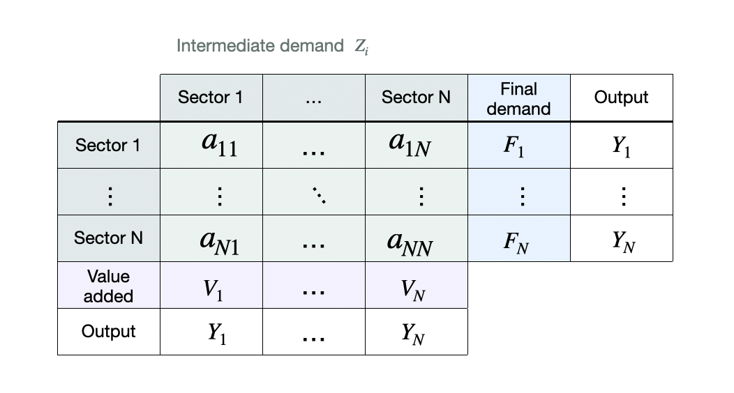
Figure 1: Scheme of the structure of a single-country input-output table [4, 3, 28].

Iterating the identity in (2), one obtains an infinite sequence of terms reflecting the use of sector $i$’s output at different level in the value chain

$$Y_{i}=F_{i}+\sum_{j=1}^{N}d_{ij}F_{j}+\sum_{j=1}^{N}\sum_{k=1}^{N}d_{ik}d_{kj}F_{j}+\dots\ .$$ (3)

Using the matrix geometric series $\sum_{k\geq 0}D^{k}=[\mathds{1}_{N}-D]^{-1}$, we can eventually rewrite (3) as

$${\bm{Y}}=[\mathds{1}_{N}-D]^{-1}{\bm{F}}\ ,$$ (4)

where $\mathds{1}_{N}$ is the $N\times N$ identity matrix, $D=(d_{ij})$ is the matrix of dollar values, and $\bm{F}$ the column vector of final demands.

Antràs and Chor [5] therefore proposed the following measure of upstreamness of the $i$-th industry, by multiplying each of the terms in (3) by their distance from final use, and dividing by $Y_{i}$

$$U_{1i} =1\cdot\frac{F_{i}}{Y_{i}}+2\cdot\frac{\sum_{j=1}^{N}d_{ij}F_{j}}{Y_{i}}$$

$$+3\cdot\frac{\sum_{j,k=1}^{N}d_{ik}d_{kj}F_{j}}{Y_{i}}+\dots=\frac{([\mathds{1}_{N}-D]^{-2}{\bm{F}})_{i}}{Y_{i}}\ ,$$ (5)

where $(\cdot)_{i}$ indicates the $i$-th component of the vector.

Inserting (4) into (5), we can rewrite the upstreamness vector as

$${\bm{U}_{1}}=[\mathds{1}_{N}-A_{U}]^{-1}{\bm{1}}\ ,$$ (6)

where

$$A_{U}=Y^{-1}A=\begin{pmatrix}\frac{a_{11}}{Y_{1}}&\cdots&\frac{a_{1N}}{Y_{1}}\\ \vdots&\ddots&\vdots\\ \frac{a_{N1}}{Y_{N}}&\cdots&\frac{a_{NN}}{Y_{N}}\end{pmatrix}$$ (7)

and $Y=\mathrm{diag}(Y_{1},\ldots,Y_{N})$. The matrix $A_{U}$ has therefore non-negative elements, and is row-substochastic ($\sum_{j}(A_{U})_{ij}\leq 1$ for all sectors $j$) because $(A_{U})_{ij}=d_{ij}Y_{j}/Y_{i}$ is the share of sector $i$’s total output that is purchased by industry $j$.

The upstreamness is defined in such a way that terms of the sum that are further upstream in the value chain have larger weight. By construction $U_{1i}\geq 1$ and is precisely equal to $1$ if no output of industry $i$ is used as input to other industries, that is the output of industry $i$ is only used to satisfy the final demand.

Antràs et al. [29] later established an equivalence between their upstreamness measure and a measure – defined in a recursive fashion – of the “distance” of an industry from the final demand proposed independently by Fally [7]. Fally’s upstreamnsess $U_{2}$ is defined as follows:

$$U_{2i}=1+\sum_{j=1}^{N}\frac{d_{ij}Y_{j}}{Y_{i}}U_{2j}\ .$$ (8)

The idea is that $\bm{U}_{2}$ aggregates information on the extent to which a sector in a given country produces goods that are sold directly to final consumers or that are sold to other sectors that themselves sell largely to final consumers. Sectors selling a large share of their output to relatively upstream industries should be therefore relatively upstream themselves. Using the fact that $d_{ij}Y_{j}=a_{ij}$ we have again that

$${{\bm{U}}_{2}}=[\mathds{1}_{N}-A_{U}]^{-1}{{\bm{1}}}\ ,$$ (9)

where $A_{U}$ is defined in (7). In [8] an application of those measures for the analysis of empirical data on global value chains is presented.

On the input-side, there is an accounting identity that sector $i$’s total input $Y_{i}$ be equal to the value of its primary inputs (value added) $V_{i}$ plus its intermediate input purchases from all other sectors:

$$Y_{i}=V_{i}+Z_{i}=V_{i}+\sum_{j=1}^{N}a_{ji}=V_{i}+\sum_{j=1}^{N}d_{ji}Y_{j}\ ,$$ (10)

or in vector/matrix form

$${\bm{Y}}=[\mathds{1}_{N}-D^{T}]^{-1}{\bm{V}}\ .$$ (11)

Similarly to [5] (see (5)), Miller and Temurshoev [6] introduced the so-called downstreamness measuring the average distance between suppliers of primary inputs and sectors as input purchaser along the input demand supply chain as follows

$$D_{1i} =1\cdot\frac{V_{i}}{Y_{i}}+2\cdot\frac{\sum_{j=1}^{N}V_{j}d_{ji}}{Y_{i}}+$$

$$+3\cdot\frac{\sum_{j,k=1}^{N}V_{j}d_{jk}d_{ki}}{Y_{i}}+\dots=\frac{([\mathds{1}_{N}-D^{T}]^{-2}{\bm{V}})_{i}}{Y_{i}}\ .$$ (12)

As before, using (11), we obtain

$${\bm{D}}_{1}=[\mathds{1}_{N}-A_{D}]^{-1}{\bm{1}}$$ (13)

with

$$\ \ {\rm with}\ A_{D}=(AY^{-1})^{T}=\begin{pmatrix}\frac{a_{11}}{Y_{1}}&\cdots&\frac{a_{N1}}{Y_{1}}\\ \vdots&\ddots&\vdots\\ \frac{a_{1N}}{Y_{N}}&\cdots&\frac{a_{NN}}{Y_{N}}\end{pmatrix}\ .$$ (14)

Also the matrix $A_{D}$ has therefore non-negative elements, and is row-substochastic ($\sum_{j}(A_{D})_{ij}\leq 1$ for all sectors $j$). It is worth noting that by construction the matrices $A_{U}$ and $A_{D}$ share the diagonal elements $a_{ii}/Y_{i}$.

Finally, as in the upstreamness case, also for the downstreamness, Fally [7] introduced an analogous iterative definition of the form

$$D_{2i}=1+\sum_{j=1}^{N}d_{ji}D_{2j}\ ,$$ (15)

which can be again mapped with simple manipulations into Eq. (13) using $Y_{i}d_{ji}=a_{ji}$.

The I-O Table in Fig. 1 can be modified in a conceptually simple way to account for inter-country trade by accommodating different inter-sectorial blocks (one for each country) – see scheme in Fig. 1 of [8]. The upstreamness (or downstreamness) of a country is then a suitably averaged (aggregate) version of the upstreamness (or downstreamness) of all industrial sectors of that country. In principle, there are two different ways to perform this aggregation. First, one could take the “giant” I-O table and collapse its entries at the country-by-country level by computing the total purchases of intermediate inputs by country $j$ from country $i$ – and then compute the upstreamness and the downstreamness on the collapsed (aggregate) table. Or, one could keep working with the giant table, compute the upstreamness and the downstreamness of industrial sectors within a country, and then perform a suitable average of those at country level. In [8], the two approaches were found to deliver extremely highly correlated country-level indices of GVC positioning.

3 The random model

Our randomized model is based on the closed-economy paradigm described in the previous section, and it assumes that the $N\times N$ matrices $A_{U}$ and $A_{D}$ (defined in Eqs. (7) and (14), respectively) are generated from a random interaction matrix $A$ between sectors, i.e. without any structural information about the underlying dynamics of goods and prices apart from the constraint that their entries be non-negative, and that the matrices be row-substochastic. See subsection 3.2 for the precise definition of the random model.

3.1 Covariance and slope

Assuming therefore that the underlying model for the interaction matrix $A$ is random, the covariance between the upstreamness $(\bm{U}_{1})_{i}$ and downstreamness $(\bm{D}_{1})_{i}$ (defined in Eqs. (6) and (13), respectively) of the same $i$-th sector is

$$\mathrm{Cov} ((\bm{U}_{1})_{i},(\bm{D}_{1})_{i})=$$

$$=\mathbb{E}\left[(\bm{U}_{1})_{i}(\bm{D}_{1})_{i}\right]-\mathbb{E}[(\bm{U}_{1})_{i}]\mathbb{E}[(\bm{D}_{1})_{i}]\ ,$$ (16)

where the expectation $\mathbb{E}[\cdot]$ is taken w.r.t. the joint probability density function (pdf) of the entries of the matrix $A$ (from which $A_{U}$ and $A_{D}$ are constructed). Since the upstreamness and downstreamness are defined in terms of a complicated matrix inversion, computing the covariance in Eq. (16) is a non-trivial task even for very simple joint pdfs of the entries of $A$.

However, we can take advantage of the results in Ref. [30, 31], which demonstrated that the “true” upstreamness and downstreamness (as defined in Eqs. (6) and (13), respectively) are individually correlated with simpler rank-1 estimators

$$\tilde{U}_{i} =1+\frac{r_{i}}{1-(1/N)\sum_{j}r_{j}}$$ (17)

$$\tilde{D}_{i} =1+\frac{r_{i}^{\prime}}{1-(1/N)\sum_{j}r_{j}^{\prime}}\ ,$$ (18)

where $r_{i}=\sum_{j}(A_{U})_{ij}$ are the row sums of $A_{U}$, and $r_{i}^{\prime}=\sum_{j}(A_{D})_{ij}$ are the row sums of $A_{D}$.

It is therefore sufficient to compute the covariance between the simpler estimators

$$\mathrm{Cov}(\tilde{U}_{i},\tilde{D}_{i})=\mathbb{E}[\tilde{U}_{i}\tilde{D}_{i}]-\mathbb{E}[\tilde{U}_{i}]\mathbb{E}[\tilde{D}_{i}]$$ (19)

to draw meaningful conclusions about the covariance between upstreamness and downstreamness as originally defined.

Noting that the quantities $(1/N)\sum_{j}r_{j}$ and $(1/N)\sum_{j}r_{j}^{\prime}$ quickly converge to their non-fluctuating averages $\mathbb{E}[r]$ and $\mathbb{E}[r^{\prime}]$ by virtue of the Law of Large Numbers (LLN), we make the further simplifying move to replace these quantities with their non-fluctuating averages directly in the calculation of the covariance Eq. (19). Therefore, our covariance of interest reduces to the following object

$$\mathcal{C}_{N}=\frac{\mathbb{E}[rr^{\prime}]-\mathbb{E}[r]\mathbb{E}[r^{\prime}]}{(1-\mathbb{E}[r])(1-\mathbb{E}[r^{\prime}])}\ ,$$ (20)

where we omitted the $i$-dependence (as every sector is statistically equivalent to any other in our random models). Therefore, $r$ and $r^{\prime}$ can be viewed as the sum of, say, the first row of $A_{U}$ and $A_{D}$, respectively.

We check with numerical simulations in Figs. 2 and 3 that indeed our conclusions are not affected by the fact that we considered simpler estimators in lieu of the original observables, as the former are perfectly correlated with the latter.

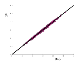
Figure 2: Scatter plot of the approximate upstreamness (Eq. (17)) vs. the “true” upstreamness $(\bm{U}_{1})_{i}$ for our random model with exponential disorder. The parameters used are $\mu=1$, $\mu_{F}=0.1$, $N=100$, $i=7$. There are $1000$ pairs of points in the figure, each obtained from a different instance of the random matrix $A$ with exponential disorder.

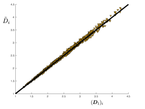
Figure 3: Scatter plot of the approximate downstreamness (Eq. (18)) vs. the “true” downstreamness $(\bm{D}_{1})_{i}$ for our random model with exponential disorder. The parameters used are $\mu=1$, $\mu_{F}=0.01$, $N=100$, $i=7$. There are $1000$ pairs of points in the figure, each obtained from a different instance of the random matrix $A$ with exponential disorder.

The slope $S$ of the scatter plot between $\tilde{D}_{i}$ and $\tilde{U}_{i}$ is easily determined from Eq. (19) by assuming first that there be a linear relation between the two, $\tilde{D}_{i}=S\tilde{U}_{i}$, and substituting in the expression for the covariance Eq. (19) we get

$$\mathrm{Cov}(\tilde{U}_{i},\tilde{D}_{i})=S\left\{\mathbb{E}[\tilde{U}_{i}^{2}]-\mathbb{E}[\tilde{U}_{i}]^{2}\right\}\ ,$$ (21)

from which we deduce

$$S=\frac{\mathrm{Cov}(\tilde{U}_{i},\tilde{D}_{i})}{\mathrm{Var}[\tilde{U}_{i}]}\ ,$$ (22)

where $\mathrm{Var}[\tilde{U}_{i}]=\mathbb{E}[\tilde{U}_{i}^{2}]-\mathbb{E}[\tilde{U}_{i}]^{2}$ is the variance of the approximate upstreamness.

Making again the further approximation that $(1/N)\sum_{j}r_{j}$ is replaced with its non-fluctuating average $\mathbb{E}[r]$ by virtue of the Law of Large Numbers, and after simple algebra from Eq. (18), we have that the slope $S$ can be approximated by

$$S=\frac{\mathcal{C}_{N}\left(1-\mathbb{E}[r]\right)^{2}}{\mathbb{E}[r^{2}]-\mathbb{E}[r]^{2}}\ .$$ (23)

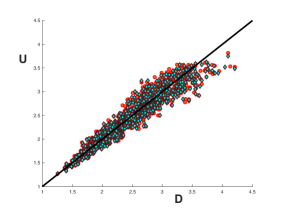
Figure 4: Scatter plot between upstreamness and downstreamness of sector $i=7$ for the $N=200$ random model with exponential disorder with parameters $\mu=1$, $\mu_{F}=0.005$. Each of the $1000$ blue [red] points is obtained from one instance of the random “source” matrix $A$, and represents the pair of values ($(\bm{U}_{1})_{i},(\bm{D}_{1})_{i}$) [($\tilde{U}_{i},\tilde{D}_{i}$), respectively]. The thick black line has slope $+1$.

3.2 Model definition

In the random model we consider that the entries of $A$ are drawn independently from an exponential probability density function (pdf) $p(a)=\mu\exp(-\mu a)$ with mean $1/\mu$. As such, the entries of $A$ are all positive, and no economic or empirically motivated information whatsoever is injected in the construction of $A$. The final demand values $F_{i}$ $(i=1,\ldots,N)$ are further modeled as i.i.d. exponential random variables with mean $1/\mu_{F}$.

From the matrix $A$, we construct the matrices $A_{U}$ and $A_{D}$ (see Eq. (7) and (14), together with the definition of $Y_{i}$ in Eq. (1)) as

$$(A_{U})_{ij} =\frac{a_{ij}}{\sum_{j}a_{ij}+F_{i}}$$ (24)

$$(A_{D})_{ij} =\frac{a_{ji}}{\sum_{j}a_{ij}+F_{i}}\ ,$$ (25)

where we used that $\sum_{j}a_{ij}+F_{i}=\sum_{j}a_{ji}+V_{i}$ for all $i$, as follows from the accounting identity. Therefore, provided that $\mu_{F}$ is sufficiently small, both $A_{U}$ and $A_{D}$ as defined above have non-negative elements, and are row sub-stochastic (as they should).

For each instance of the random matrix $A$ and of the vector of final demands $\bm{F}$, we construct the matrices $A_{U}$ and $A_{D}$ as above, and from those we compute the pairs $(\bm{U}_{1})_{i},(\bm{D}_{1})_{i}$ and $\tilde{U}_{i},\tilde{D}_{i}$ for any sector $i$ that we choose. These are all random variables, whose pairwise covariance is of interest in this paper.

4 Results

Our results are summarized in the theorem and corollary below. We show that even in our completely random model (with no economic or empirically motivated information whatsoever injected in constructing the I/O table), the upstreamness and downstreamness of an industrial sector of a single country are necessarily positively correlated, and that for any $N$ the slope of the scatter plot between the two is always equal to $+1$.

In Figs. 5 and 6 we further numerically check that our results do not crucially depend on the specific choice of the way the random matrices $A_{U}$ and $A_{D}$ are generated, so the positive correlation between upstreamness and downstreamness of economic sectors – and their correlation slope being $+1$ – seem to be very robust results and rather insensitive to the fine details of the inter-sectorial I/O matrix.

Theorem 1.

Let $N\times N$ matrices be defined as

$$(A_{U})_{ij} =\frac{a_{ij}}{\sum_{j}a_{ij}+F_{i}}$$ (26)

$$(A_{D})_{ij} =\frac{a_{ji}}{\sum_{j}a_{ij}+F_{i}}\ ,$$ (27)

where $a_{ij}$ are i.i.d. variables drawn from an exponential pdf $p(a)=\mu\exp(-\mu a)$, and the $F_{i}$’s are i.i.d. variables drawn from an exponential pdf $p_{F}(F)=\mu_{F}\exp(-\mu_{F}F)$ with $\mu_{F}\ll\mu$ to ensure that $A_{U}$ and $A_{D}$ are row sub-stochastic. Let $r=\sum_{j}(A_{U})_{1j}$ and $r^{\prime}=\sum_{j}(A_{D})_{1j}$. Then the simplified covariance between upstreamness and downstreamness (see Eq. (20))

$$\mathcal{C}_{N}(\mu,\mu_{F})=\frac{\mathbb{E}[rr^{\prime}]-\mathbb{E}[r]\mathbb{E}[r^{\prime}]}{(1-\mathbb{E}[r])(1-\mathbb{E}[r^{\prime}])}$$ (28)

is given by the exact formula $\mathcal{C}_{N}(\mu,\mu_{F})=-\mathcal{N}_{N}(\phi)/\mathcal{D}_{N}(\phi)$, where

$$\mathcal{N}_{N}(\phi)=(\phi-1)\left[N(\phi-1)\mathrm{B}(1,N+1)^{2}\,_{2}F_{1}(1,N+1;N+2;\phi){}^{2}+(N-1)N(\phi-1)\mathrm{B}(1,N+1)\,_{2}F_{1}(1,N+1;N+2;\phi)(\mathrm{B}(1,N)\,_{2}F_{1}(1,N;N+1;\phi)+1)+(N+1)(\phi-1)\mathrm{B}(1,N+2)\,_{2}F_{1}(1,N+2;N+3;\phi)+N\right]$$

$$\mathcal{D}_{N}(\phi)=((N-1)(\phi-1)\mathrm{B}(1,N)\,_{2}F_{1}(1,N;N+1;\phi)+(\phi-1)\mathrm{B}(1,N+1)\,_{2}F_{1}(1,N+1;N+2;\phi)+1)(N(\phi-1)\mathrm{B}(1,N+1)\,_{2}F_{1}(1,N+1;N+2;\phi)+1)\ ,$$

where $\phi=1-\mu_{F}/\mu$. Here, $\mathrm{B}(x,y)=\Gamma(x)\Gamma(y)/\Gamma(x+y)$ is the Beta function, and ${}_{2}F_{1}$ is the Gaussian hypergeometric function.

Corollary 1.

In the hypotheses of Theorem 1, the slope $S(\mu,\mu_{F})$ of the scatter plot between the rank-1 estimators of downstreamness and upstreamness (see Eq. (23)) is equal to $+1$ for any $N$, irrespective of the values of $\mu,\mu_{F}$.

The proofs are deferred to the Appendix.

5 Numerical simulations

We have performed numerical simulations on our random model, generating $m$ instances of the $N\times N$ matrix $A$ with i.i.d. exponential entries with mean $1/\mu$. We also generate random vectors of final demands $\bm{F}$ of size $N$, with i.i.d. entries with mean $1/\mu_{F}$ (with $\mu_{F}\ll\mu$).

For each generated instance of the matrix $A$, we formed the matrices $A_{U}$ and $A_{D}$ (as defined in Eqs. (7) and (14)), which have by construction non-negative elements, and are row sub-stochastic.

From the matrices $A_{U}$ and $A_{D}$ so generated, we constructed the vectors of upstreamness $\bm{U}_{1}$ and downstreamness $\bm{D}_{1}$ values according to the inversion formulae Eq. (6) and (13), respectively. We then pick a certain sector index $i$ (for example, $i=7$), and for that index we compute the estimators $\tilde{U}_{i}$ and $\tilde{D}_{i}$ according to Eqs. (17) and (18) respectively.

We first show in Figs. 2 and 3 that the “true” upstreamness (downstreamness) of sector $i$ – computed from the full inversion formulae – is perfectly correlated (with correlation slope $=+1$) with its approximate estimator. It is therefore perfectly justified to use the approximate estimators (instead of the full definition) to study correlations, as those are much simpler to handle analytically.

Next, in Table 1, we report values of the “true” covariance between upstreamness and downsteamness of sector $i=7$, obtained from averaging over $m=10000$ numerically generated instances of our random model, against the values of $\mathcal{C}_{N}(\mu,\mu_{F})$ analytically computed, and we observe an excellent agreement between the two.

In Fig. 4 we further provide scatter plots of upstreamness vs. downstreamness of sector $i$ (both “true” and approximate) - where each generated instance contributes a single point to the scatter plot. Again, we observe an excellent collapse onto the diagonal line with slope $+1$, further confirming that a strong positive correlation between upstreamness and downstreamness of the same sector is a generic feature of “structure-less” matrices – provided they have non-negative entries and are sub-stochastic.

Finally, in Figs. 5 and 6 we provide the same scatter plots as in Fig. 4, but this time for the “original” matrix $A$ (and similarly for the vector $\bm{F}$) having i.i.d. non-negative entries drawn from a log-normal ($p(a)=(a\sqrt{2\pi})^{-1}\exp(-(\ln(a)-\mu^{\prime})^{2}/2)$) and uniform (with mean $1/\mu$ and $1/\mu_{F}$) pdf, respectively. Although we do not provide analytical results for these cases, these plots further confirm that the positive correlation with slope $+1$ between upstreamness and downstreamness keeps holding irrespective of the precise details of the way the “source” matrix $A$ is generated – provided that $A_{U}$ and $A_{D}$ are non-negative and sub-stochastic.

Table 1: Covariance between Upstreamness and Downstreamness in the random model for $i=7$ and taken over $m=10000$ samples

$\mu$	$\mu_{F}$	$N$	$\mathrm{Cov}((\bm{U}_{1})_{i},(\bm{D}_{1})_{i})$	$\mathcal{C}_{N}(\mu,\mu_{F})$
1	0.001	200	0.10450	0.10385
2	0.005	400	0.30415	0.29494
3	0.001	300	0.06136	0.06158
1.2	0.001	500	0.17346	0.17260
1.5	0.003	350	0.24224	0.23955

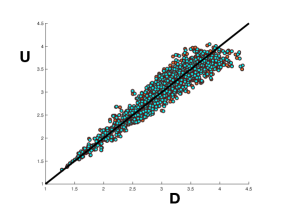
Figure 5: Scatter plot between upstreamness and downstreamness of sector $i=7$ for the $N=400$ random model with log-normal disorder with parameters $\mu^{\prime}=1$, $\mu_{F}^{\prime}=6.67$. Each of the $1000$ light blue [orange] points is obtained from one instance of the random “source” matrix $A$, and represents the pair of values ($(\bm{U}_{1})_{i},(\bm{D}_{1})_{i}$) [($\tilde{U}_{i},\tilde{D}_{i}$), respectively]. The thick black line has slope $+1$.

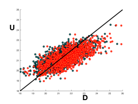
Figure 6: Scatter plot between upstreamness and downstreamness of sector $i=7$ for the $N=400$ random model with uniform disorder with parameters $\mu=1$, $\mu_{F}=0.05$. Each of the $1000$ light blue [orange] points is obtained from one instance of the random “source” matrix $A$, and represents the pair of values ($(\bm{U}_{1})_{i},(\bm{D}_{1})_{i}$) [($\tilde{U}_{i},\tilde{D}_{i}$), respectively]. The thick black line has slope $+1$.

6 Discussion

In summary, we have considered a random Input/Output matrix $A$ that mimics a closed economy composed of $N$ economic sectors. We showed analytically that the resulting upstreamness and downstreamness of a given sector are generically positively correlated, with a slope of the scatter plot between the two equal to $+1$, if the entries of the matrix $A$ are independently drawn from an exponential pdf. We also showed numerically that our results do not depend very strongly on the pdf of matrix entries. At least at the level of single countries, our work provides a comforting “proof of principle” that a strong positive correlation between upstreamness and downstreamness of individual sectors as originally defined (see Eqs. (6) and (13)) is bound to materialize even on a structure-less and zero-information I-O matrix: one would have to try very hard to concoct an I-O matrix so extraordinary and finely tuned, that such correlations were not observed.

Although derived in the context of a closed-economy I-O table (see Fig. 1), our results are nevertheless also relevant to the more general setting of international trade considered in [8] and the puzzling correlation highlighted thereof, for a few reasons: (i) the “giant” I-O matrix that includes inter-country trade blocks satisfies the same constraints (non-negative entries, and row-stochasticity) as the single-country one (and thus as well as the random model we presented). (ii) Preliminary numerical experiments played on random $A$ matrices with a block structure similar to the giant I-O matrix did not present evidence of any combination of heterogeneity in the distribution of entries, sparsity patterns of blocks, or aggregation of outcomes (either before or after the country upstreamness/downstreamness were computed) that was ever able to break the robust positive correlation between upstreamness and downstreamness observed again in that more general setting – this time, at the country level – and entirely akin to the simpler setting described in this paper. (iii) The model considered here – after a trivial re-interpretation of the matrix entries – is at the very least expected to mimic rather accurately what would happen in the more general inter-country setting in the two extreme cases of zero and infinite trade barriers between different countries. In the former case, the “giant” I-O matrix will have inter-country and intra-country blocks that do not differ much (statistically), therefore – after country-wise aggregation – the resulting $A$ matrix will look very similar to the one we considered in this paper. In the latter case, the “giant” I-O matrix will be block-diagonal – with inter-country blocks full of zeros due to the absence of trade – with each non-zero (intra-country) block being an independent replica of the closed economy model proposed here. While a deeper investigation of the intermediate trade barriers setting in the random “giant” model is surely needed, the aforementioned observations sharply point towards the observed correlation between upstreamness and downstreamness also at country level being simply due to structural and unavoidable algebraic constraints that I-O tables and their surrogates must satisfy.

Our results rest on the following assumptions and simplifications:

1. The correlation between “true” upstreamness and downstreamness of a sector can be faithfully probed by using the rank-$1$ approximants defined in [30, 31]. This assumption was tested on empirical I/O data in [30, 31], and on the random model here in Figs. 2 and 3, by showing that the “true” upstreamness (or downstreamness) is indeed perfectly correlated with its rank-$1$ approximant. Such rank-$1$ approximation could only become less reliable if the true Input/Output matrix were exceedingly sparse, i.e. with a very large number of zero entries (see discussion in [31, 32, 33]), a fact that does not often materialize in practice. By considering national I-O tables available from the 2013 release of the WIOD [4], we indeed obtain quite high average densities – between 0.92 and 0.93 across 40 countries for the years 1995-2011. We have further checked that a moderate sparsification of our random model does not qualitatively change our conclusions, however in future experiments it will be appropriate to test the consequences of sparsity more thoroughly.

2. We have assumed that the entries of the matrix $A$ were independent and identically distributed (i.i.d.). Some preliminary results (not shown) where this assumption has been relaxed indicate that heterogeneity in the pdfs of the entries of $A$ may not play a major role and is generally insufficient to change the conclusions of our analysis.

3. We used some simplifications (for instance, appealing to the LLN) to make some progress in the analytical calculations. All approximations are controlled and have been carefully tested.

Apart from performing a more thorough study on the effect of sparsity and heterogeneity in random models of I-O tables, in future studies it will be interesting to try to compute analytically the full covariance Eq. (16) for our random model and for various different pdfs of the entries of the I/O matrix $A$, i.e. without employing any rank-$1$ proxy and/or LLN approximations. This task will require handling the average of (products of) inverse matrices (coming from the definitions of upstreamness and downstreamness, see Eq. (6) and (13)), which is possible in some cases using techniques from statistical physics [30].

Appendix A Derivation of Theorem 1 and Corollary 1

We need to compute $\mathbb{E}[r]$, $\mathbb{E}[r^{\prime}]$ and $\mathbb{E}[rr^{\prime}]$ separately. We have

$$\mathbb{E}[r]=\int_{0}^{\infty}\prod_{i=1}^{N}da_{i}p(a_{i})\int_{0}^{\infty}dF~{}p_{F}(F)\frac{\sum_{k}a_{k}}{\sum_{k}a_{k}+F}\ ,$$ (29)

where for simplicity we denoted $a_{k}\equiv a_{1k}$ and $F\equiv F_{1}$. Using the identity

$$\frac{1}{\xi}=\int_{0}^{\infty}ds~{}e^{-\xi s}\qquad\xi>0$$ (30)

we have

$$\mathbb{E}[r] =\mu^{N}\mu_{F}\int_{0}^{\infty}\prod_{i=1}^{N}da_{i}\int_{0}^{\infty}dFds~{}\sum_{k}a_{k}\times$$

$$\times e^{-\mu\sum_{k}a_{k}-\mu_{F}F-s(\sum_{k}a_{k}+F)}$$

$$=\mu^{N}\mu_{F}N\int_{0}^{\infty}ds\left[\int_{0}^{\infty}dae^{-\mu a-sa}\right]^{N-1}\times$$

$$\times\int_{0}^{\infty}dy~{}ye^{-\mu y-sy}\int_{0}^{\infty}dFe^{-\mu_{F}F-sF}$$

$$=\boxed{\mu^{N}\mu_{F}NJ(N+1)}$$ (31)

where

$$J(k) =\int_{0}^{\infty}ds\frac{1}{(\mu+s)^{k}}\frac{1}{\mu_{F}+s}=$$

$$=\frac{1}{\mu^{k}}\int_{0}^{\infty}dt(1+t)^{-1}\left(1+\frac{\mu_{F}}{\mu}t\right)^{-k}=$$

$$=\frac{1}{\mu^{k}}\mathrm{B}(1,k)~{}_{2}F_{1}(k,1;k+1;1-\mu_{F}/\mu)$$ (32)

from [34], formula 3.197.5 (pag. 335) with $\lambda=1$, $\nu=-1$, $\alpha=\mu_{F}/\mu$ and $\tilde{\mu}=-k$. Here, $\mathrm{B}(\cdot,\cdot)$ is the Beta function, and ${}_{2}F_{1}$ is a hypergeometric function.

Similarly

$$\mathbb{E} [r^{\prime}]=\mu^{2N-1}\mu_{F}\int_{0}^{\infty}\prod_{i=1}^{N}da_{i}p(a_{i})\prod_{j=2}^{N}db_{j}p(b_{j})\times$$

$$\times\int_{0}^{\infty}dF~{}p_{F}(F)\frac{a_{1}+\sum_{k\geq 2}b_{k}}{\sum_{k}a_{k}+F}$$

$$=\boxed{\mu^{2N-1}\mu_{F}\left[\frac{1}{\mu^{N-1}}J(N+1)+\frac{N-1}{\mu^{N}}J(N)\right]}\ ,$$ (33)

where for simplicity we denoted $a_{1j}\equiv a_{j}$ (for $j=1,\ldots,N$), and $a_{k1}\equiv b_{k}$ (for $k=2,\ldots,N$). To prove this, we write

$$\mathbb{E}[r^{\prime}]=\mu^{2N-1}\mu_{F}[I_{1}+I_{2}]\ ,$$ (34)

where

$$I_{1} =\int_{0}^{\infty}ds\left[\int_{0}^{\infty}dxe^{-\mu x-sx}\right]^{N-1}\int_{0}^{\infty}dy~{}ye^{-\mu y-sy}$$

$$\times\left[\int_{0}^{\infty}dz~{}e^{-\mu z}\right]^{N-1}\int_{0}^{\infty}dFe^{-\mu_{F}F-sF}$$

$$=\frac{1}{\mu^{N-1}}\int_{0}^{\infty}ds\frac{1}{(\mu+s)^{N+1}(\mu_{F}+s)}=\boxed{\frac{J(N+1)}{\mu^{N-1}}}$$ (35)

and

$$I_{2} =(N-1)\int_{0}^{\infty}ds\left[\int_{0}^{\infty}dx~{}e^{-\mu x-sx}\right]^{N}\times$$

$$\times\int_{0}^{\infty}dFe^{-\mu_{F}F-sF}\left[\int_{0}^{\infty}dye^{-\mu y}\right]^{N-2}\times$$

$$\int_{0}^{\infty}dz~{}ze^{-\mu z}=\frac{N-1}{\mu^{N}}\int_{0}^{\infty}ds\frac{1}{(\mu+s)^{N}(\mu_{F}+s)}$$

$$=\boxed{\frac{N-1}{\mu^{N}}J(N)}\ .$$

Finally

$$\mathbb{E}[rr^{\prime}]=\mu^{2N-1}\mu_{F}\int_{0}^{\infty}\prod_{i=1}^{N}da_{i}p(a_{i})\prod_{j=2}^{N}db_{j}p(b_{j})dF$$

$$\frac{\sum_{\ell}a_{\ell}}{\sum_{k}a_{k}+F}\frac{a_{1}+\sum_{k\geq 2}b_{k}}{\sum_{k}a_{k}+F}=$$

$$=\mu^{2N-1}\mu_{F}\left[\frac{2}{\mu^{N-1}}L(N+2)+\frac{N-1}{\mu^{N}}L(N+1)\right.$$

$$\left.+\frac{N-1}{\mu^{N-1}}L(N+2)+\frac{(N-1)^{2}}{\mu^{N}}L(N+1)\right]\ ,$$ (36)

where

$$L(k) =\int_{0}^{\infty}dsdt\frac{1}{\mu_{F}+s+t}\frac{1}{(\mu+s+t)^{k}}=$$

$$=\frac{\mu^{1-k}}{k-1}-\mu_{F}J(k)\ .$$ (37)

Eq. (36) follows from writing $\sum_{\ell}a_{\ell}=a_{1}+\sum_{\ell\neq 1}a_{\ell}$, and applying the “lifting-up” identity (30) twice, which yields

$$\mathbb{E}[rr^{\prime}]=\mu^{2N-1}\mu_{F}[K_{1}+K_{2}+K_{3}+K_{4}]\ ,$$ (38)

where

$$K_{1} =\int dx_{1}\cdots dx_{N}dF_{1}dy_{2}\cdots dy_{N}dsdt$$

$$e^{-\mu\sum_{k}x_{k}-\mu\sum_{k\geq 2}y_{k}-\mu_{F}F_{1}}x_{i}^{2}\times$$

$$\times e^{-s(\sum_{k}x_{k}+F_{1})-t(\sum_{k}x_{k}+F_{1})}=$$

$$=\frac{1}{\mu^{N-1}}\int dsdt\frac{1}{\mu_{F}+s+t}\left[\int dx~{}e^{-\mu x-(s+t)x}\right]^{N-1}$$

$$\times\int dx~{}x^{2}e^{-\mu x-(s+t)x}$$

$$=\frac{2}{\mu^{N-1}}\int_{0}^{\infty}dsdt\frac{1}{\mu_{F}+s+t}\frac{1}{(\mu+s+t)^{N+2}}=$$

$$=\boxed{\frac{2}{\mu^{N-1}}L(N+2)}\ .$$ (39)

$$K_{2} =\int dx_{1}\cdots dx_{N}dF_{1}dy_{2}\cdots dy_{N}dsdt$$

$$\times e^{-\mu\sum_{k}x_{k}-\mu\sum_{k\geq 2}y_{k}-\mu_{F}F_{1}}x_{i}\sum_{k\geq 2}y_{k}\times$$

$$\times e^{-s(\sum_{k}x_{k}+F_{1})-t(\sum_{k}x_{k}+F_{1})}=$$

$$=(N-1)\int dsdt\frac{1}{\mu_{F}+s+t}\left[\int dx~{}e^{-\mu x-(s+t)x}\right]^{N-1}$$

$$\times\int dx~{}xe^{-\mu x-(s+t)x}$$

$$\times\left[\int dye^{-\mu y}\right]^{N-2}\int dy~{}ye^{-\mu y}$$

$$=\frac{N-1}{\mu^{N}}\int_{0}^{\infty}dsdt\frac{1}{\mu_{F}+s+t}\frac{1}{(\mu+s+t)^{N+1}}=$$

$$=\boxed{\frac{N-1}{\mu^{N}}L(N+1)}\ .$$ (40)

$$K_{3} =\int dx_{1}\cdots dx_{N}dF_{1}dy_{2}\cdots dy_{N}dsdt$$

$$\times e^{-\mu\sum_{k}x_{k}-\mu\sum_{k\geq 2}y_{k}-\mu_{F}F_{1}}x_{i}\sum_{\ell\neq i}x_{\ell}\times$$

$$\times e^{-s(\sum_{k}x_{k}+F_{1})-t(\sum_{k}x_{k}+F_{1})}=$$

$$=(N-1)\int dsdt\frac{1}{\mu_{F}+s+t}\left[\int dx~{}xe^{-\mu x-(s+t)x}\right]^{2}$$

$$\times\left[\int dx~{}e^{-\mu x-(s+t)x}\right]^{N-2}\times\left[\int dye^{-\mu y}\right]^{N-1}$$

$$=\frac{N-1}{\mu^{N-1}}\int_{0}^{\infty}dsdt\frac{1}{\mu_{F}+s+t}\frac{1}{(\mu+s+t)^{N+2}}=$$

$$=\boxed{\frac{N-1}{\mu^{N-1}}L(N+2)}\ .$$ (41)

$$K_{4} =\int dx_{1}\cdots dx_{N}dF_{1}dy_{2}\cdots dy_{N}dsdt$$

$$\times e^{-\mu\sum_{k}x_{k}-\mu\sum_{k\geq 2}y_{k}-\mu_{F}F_{1}}\sum_{k\geq 2}y_{k}\sum_{\ell\neq i}x_{\ell}\times$$

$$\times e^{-s(\sum_{k}x_{k}+F_{1})-t(\sum_{k}x_{k}+F_{1})}=$$

$$=(N-1)^{2}\int dsdt\frac{1}{\mu_{F}+s+t}$$

$$\times\left[\int dx~{}xe^{-\mu x-(s+t)x}\right]\left[\int dx~{}e^{-\mu x-(s+t)x}\right]^{N-1}$$

$$\times\left[\int dye^{-\mu y}\right]^{N-2}\int dy~{}ye^{-\mu y}$$

$$=\frac{(N-1)^{2}}{\mu^{N}}\int_{0}^{\infty}dsdt\frac{1}{\mu_{F}+s+t}\frac{1}{(\mu+s+t)^{N+1}}=$$

$$=\boxed{\frac{(N-1)^{2}}{\mu^{N}}L(N+1)}\ .$$ (42)

Collecting all terms and simplifying, we arrive at the formula announced in Theorem 1. Plotting the covariance formula as a function of $N$ for different values of $\mu,\mu_{F}$ reveals that the covariance is always positive and increasing (see Fig. 7).

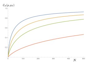
Figure 7: Covariance $\mathcal{C}_{N}(\mu,\mu_{F})$ between the approximate upstreamness and downstreamness for the random model (exact formula in Theorem 1). The parameters $(\mu,\mu_{F})$ are $(1,0.1)$ (blue), $(2,0.1)$ (orange), $(2,0.05)$ (green), $(2,0.01)$ (red).

To prove the Corollary 1, we need to further compute $\mathbb{E}[r^{2}]$ and then simplify the resulting expression for the slope (23), yielding a slope $=+1$ for any $N$.

$$\mathbb{E}[r^{2}]=\int_{0}^{\infty}\prod_{i=1}^{N}da_{i}p(a_{i})\int_{0}^{\infty}dF~{}p_{F}(F)\left[\frac{\sum_{k}a_{k}}{\sum_{k}a_{k}+F}\right]^{2}$$

$$=\mu^{N}\mu_{F}\int d\bm{a}dFds~{}se^{-\mu\sum_{k}a_{k}-\mu_{F}F}\times$$

$$\left(\sum_{k}a_{k}\right)^{2}e^{-s(\sum_{k}a_{k}+F)}$$

$$=\mu^{N}\mu_{F}\left[N\int d\bm{a}dFds~{}se^{-\mu\sum_{k}a_{k}-\mu_{F}F}a_{1}^{2}e^{-s(\sum_{k}a_{k}+F)}+\right.$$

$$+\left.(N^{2}-N)\int d\bm{a}dFds~{}se^{-\mu\sum_{k}a_{k}-\mu_{F}F}a_{1}a_{2}e^{-s(\sum_{k}a_{k}+F)}\right]$$

$$=\mu^{N}\mu_{F}N\int_{0}^{\infty}ds~{}s\left[\int dxe^{-\mu x-sx}\right]^{N-1}\int dy~{}y^{2}e^{-\mu y-sy}\times$$

$$\times\int dFe^{-\mu_{F}F-sF}+\mu^{N}\mu_{F}(N^{2}-N)\int_{0}^{\infty}ds~{}s\times$$

$$\times\left[\int dxe^{-\mu x-sx}\right]^{N-2}\left[\int dy~{}ye^{-\mu y-sy}\right]^{2}\int dFe^{-\mu_{F}F-sF}$$

$$=2\mu^{N}\mu_{F}N\int_{0}^{\infty}ds\frac{s}{(\mu+s)^{N+2}}\frac{1}{\mu_{F}+s}+$$

$$+\mu^{N}\mu_{F}(N^{2}-N)\int_{0}^{\infty}ds\frac{s}{(\mu+s)^{N+2}}\frac{1}{\mu_{F}+s}$$

$$=\boxed{\mu^{N}\mu_{F}(N^{2}+N)L(N+2)}\blacksquare$$

References

- [1] W. Leontief (1986). Input-output economics. Oxford University Press.
- [2] W. Leontief (1936). Quantitative Input-Output Relations in the Economic System of the United States. Rev. Econ. Stat. 18, pp. 105–125.
- [3] United Nations Department for Economic and Social Affairs Statistics Division (1999). Handbook of Input-Output Table Compilation and Analysis.
- [4] M. P. Timmer, E. Dietzenbacher, B. Los, R. Stehrer, and G. J. de Vries (2015). An Illustrated User Guide to the World Input–Output Database: the Case of Global Automotive Production. Review of International Economics 23, 575–605.
- [5] P. Antràs and D. Chor (2012). Organizing the global value chain. Econometrica 81(6), 2127-2204.
- [6] R. E. Miller and U. Temurshoev (2015). Output upstreamness and input downstreamness of industries/countries in world production. International regional science review 40(5), 443-475.
- [7] T. Fally (2012). Production Staging: Measurement and Facts (unpublished).
- [8] P. Antràs and D. Chor (2018). On the measurement of upstreamness and downstreamness in global value chains. Working Paper 24185 http://www.nber.org/papers/w24185
- [9] Z. Wang, S. J. Wei, X. Yu, and K. Zhu (2017). Characterizing global value chains: production length and upstreamness. Working paper No. w23261. National Bureau of Economic Research.
- [10] B. Peterson and M. Olinick (1982). Leontief models, Markov chains, Substochastic matrices, and positive solutions of matrix equations. Mathematical modelling 3, 221-239.
- [11] J. McNerney, C. Savoie, F. Caravelli, and J. D. Farmer (2021). How production networks amplify economic growth. PNAS 119 (1) e2106031118.
- [12] J. McNerney (2012). Applications of Statistical Physics to Technology Price Evolution. Ph.D. thesis, Boston University.
- [13] P. S. M. Kop Jansen (1994). Analysis of multipliers in stochastic input-output models. Regional Science and Urban Economics 24, 55-74.
- [14] P. Kop Jansen and T. Ten Raa (1990). The choice of model in the construction of Input-Output coefficients matrices. International Economic Review 31, No. 1, pp. 213- 227.
- [15] W. D. Evans (1954). The Effect of Structural Matrix Errors on Interindustry Relations Estimates. Econometrica 22 (n. 4), pp. 461-480.
- [16] R. E. Quandt (1958). Probabilistic errors in the Leontief system. Naval Research Logistics Quarterly 5, pp. 155-170.
- [17] A. Simonovits (1975). A Note on the Underestimation and Overestimation of the Leontief Inverse. Econometrica 43, pp. 493-498.
- [18] G. R. West (1986). A stochastic analysis of an input-output model. Econometrica: Journal of the Econometric Society 54, 363-374.
- [19] H. Kogelschatz (2007). On the Solution of Stochastic input-output-Models. Discussion Paper Series n. 447, University of Heidelberg.
- [20] M. Kozicka (2019). Novel approach to stochastic Input-Output modeling. RAIRO-Oper. Res. 53, 1155–1169 https://doi.org/10.1051/ro/2018046.
- [21] J. L. Katz and R. L. Burford (1985). Shortcut formulas for output, income and employment multipliers. The Annals of Regional Science 19(2), 61-76.
- [22] R. L. Burford (1977). Regional input-output multipliers without a full IO table. The Annals of Regional Science 11(3), 21-38.
- [23] R. L. Drake (1976). A short-cut to estimates of regional input-output multipliers: methodology and evaluation. International Regional Science Review 1(2), 1-17.
- [24] P. J. Phibbs and A. J. Holsman (1981). An evaluation of the Burford Katz short cut technique for deriving input-output multipliers. The Annals of Regional Science 15(3), 11-19.
- [25] R. C. Jensen and G. J. D. Hewings (1985). Shortcut ‘Input-Output’ Multipliers: The Resurrection Problem (a Reply). Environment and Planning A 17(11), 1551-1552.
- [26] R. C. Jensen and G. J. D. Hewings (1985). Shortcut ‘input-output’ multipliers: A requiem. Environment and Planning A 17(6), 747-759.
- [27] R. L. Burford and J. L. Katz (1985). Shortcut ‘input-output’ multipliers, alive and well: Response to Jensen and Hewings. Environment and Planning A 17(11), 1541-1549.
- [28] Suganuma, K. (2016) Upstreamness in the global value chain: Manufacturing and services. In Meeting of the Japanese Economic Association at Nagoya University on June (Vol. 18, p. 19) .
- [29] P. Antràs, D. Chor, T. Fally, and R. Hillberry (2012). Measuring the Upstreamness of Production and Trade Flows. American Economic Review: Papers & Proceedings 102(3): 412–416.
- [30] S. Bartolucci, F. Caccioli, F. Caravelli, and P. Vivo (2020). Inversion-free Leontief inverse: statistical regularities in input-output analysis from partial information. Preprint arXiv:2009.06350.
- [31] S. Bartolucci, F. Caccioli, F. Caravelli, and P. Vivo (2022). Ranking influential nodes in networks from partial information. Preprint arXiv:2009.06307v5.
- [32] S. Bartolucci, F. Caccioli, F. Caravelli, and P. Vivo (2021). “Spectrally gapped” random walks on networks: a Mean First Passage Time formula. SciPost Phys. 11, 088.
- [33] M. J. Crumpton, Y. V. Fyodorov, P. Vivo (2022). Statistics of the largest eigenvalues and singular values of low-rank random matrices with non-negative entries. Preprint arXiv:2208.09430.
- [34] I. S. Gradshteyn and I. M. Ryzhik (2000). Table of Integrals, Series and Products. Academic Press; 6th edition.