Complex Discretization approximation for the full dynamics of system-environment quantum models

Abstract

The discretization approximation method used to simulate the open dynamics of the environment in continuum often suffers from recurrence, which results in inefficiency. To address this issue, this paper proposes a generalization of the discretization approximation method in the complex plane using complex Gauss quadratures. The resulting effective Hamiltonian is non-Hermitian due to the dissipative dynamics of the system. The proposed method is applied to two solvable models, namely the dephasing model and the single-excitation open dynamics in the generalized Aubry-André-Harper model. The results demonstrate that the occurrence of complex discrete modes in the environment can significantly reduce recurrence, thereby enabling the efficient and accurate simulation of open dynamics in both models.

I introduction

A quantum system is inherently connected to its surroundings, which can lead to equilibrium or a steady state. The open dynamics of a system can be approximated using the Born-Markovian approach, which assumes that the system’s present state determines its temporal evolution and is independent of its pastbreuer2002 . However, recent experimental advances have allowed physicists to investigate regimes that are not accurately modeled by the Born-Markovian approximation, such as in solid-state and artificial light-matter systems light-matter , as well as in quantum biology and chemistry quantumbc . In certain situations, nonequilibrium dynamics have been observed, which demonstrate the importance of the system’s dynamics in relation to the non-Markovianity or memory effect of its environmentnonequilibrium ; opendisorderenhance .

The study of non-Markovian dynamics presents a significant challenge, often requiring the use of perturbation expansion or numerical simulation vega2017 . One common approach is to employ projection operator techniques breuer2002 , which can yield the Nakjima-Zwanzig equation nzeqn , an integrodifferential equation with a retarded memory kernal, or the time-convolutionless master equation tcl , a time-local differential equation of first order. These equations can be used to derive effective master equations through perturbational expansion based on the strength of the system-environment coupling. Numerical simulations, such as stochastic Schrödinger equationss ss , hierarchical equations of motion hem , path integral methods pathintegral , and tensor networks pathintegral , have also been proposed to determine the open dynamics of a system. These methods involve introducing an influence functional to characterize the environmental effect on the system, thereby eliminating the degree of freedom of the environment from the dynamical equation.

An alternative method for studying open quantum systems involves incorporating the complete dynamics of both the system and its surrounding environments discretization . As the environment is continuous, its Hamiltonian and coupling to the system can be represented as integrals. To facilitate computation, orthogonal polynomials can be used to discretize these integrals, resulting in a chain representation of the total Hamiltonian. This approach enables the use of powerful numerical techniques to evaluate the full dynamics, and its efficiency and convergence have been demonstrated trivedi21 . Unlike previous methods, this approach allows for the explicit determination of the eigenfunctions of the chain Hamiltonian, thereby revealing the microscopic features of the dynamics.

The recurrence resulting from the finite dimension of chain Hamiltonian can negatively impact the efficiency and accuracy of discretization approximation. To address this issue, an effective approach is to extend the discretization approximation into the complex plane, resulting in the emergence of complex energy levels that represent dissipation in systems. This concept was initially proposed to examine resonance decay in systems with a discrete state connected to a continuum kazansky97 . The approach involves discretizing integrals in dynamical equations using Gauss quadrature rules to obtain finite summations of complex items. This results in dynamical equations that can efficiently simulate decay dynamics due to the occurrence of pseudostates with complex energies. However, this approach is highly specific and may not be applicable in more general situations.

In this paper, a generalization of the concept of discretizing the environment in continuum is presented from a fundamental perspective. The approach involves introducing orthonormalized polynomials in the complex plane and applying a unitary transformation to achieve the discretization. The resulting effective full Hamiltonian is non-Hermitian, which characterizes the dissipative dynamics in the system. By solving the Hamiltonian, the open dynamics of the system can be simulated rigorously. The paper is divided into six sections, starting with a general description of the system and environment in Section II. Section III provides a brief introduction to Gauss quadrature and implements the discretization approximation of the environment in continuum using a unitary transformation based on orthonormalized polynomials. Section IV explains how to expand the discretization approximation into the complex plane, with a focus on the introduction of complex orthonormalized polynomials based on contour integrals in the complex plane. The method is illustrated using two exactly solvable models, the dephasing model and the single-excitation open dynamics in the gAAH model. In Section V, a comprehensive discussion on the open dynamics of gAAH is presented, with a focus on the robustness of the delocalization-localization transition and the mobility edge. Finally, conclusions and further discussion are given in Section VI.

II General description of the open quantum system

A conventional method of modeling environments entails viewing them as structureless systems with an infinite degree of freedom. To be precise, the dynamics of the system and environment can be explicated by the total Hamiltonian below:

$$H = H_{s}+H_{b}+H_{int}$$ (1)

$$H_{b} = \int_{0}^{\infty}\text{d}xh(x)b^{\dagger}_{x}b_{x};$$

$$H_{\text{int}} = \sum_{n}\int_{0}^{\infty}\text{d}x\left[g(x)c^{\dagger}_{n}b_{x}+g^{*}(x)b^{\dagger}_{x}c_{n}\right],$$

in which $c_{n}$ or its Hermitian conjugate $c^{\dagger}_{n}$ represent the lowering or raising operator in system. $b^{\dagger}_{x},b_{x}$ is creation and annihilation operator of the $x$-th mode in environment. In this paper, we focus only on the bosonic environment. Thus the bosonic commutative relations

$$\left[b_{x},b^{\dagger}_{x^{\prime}}\right]=\delta\left(x-x^{\prime}\right)$$

are satisfied automatically. Assuming no loss of generality, it is posited that the Hamiltonian of the system, denoted by $H_{s}$, can be expressed in matrix form, with the subscript $n$ denoting the distinct degree of freedom within the system. The environment is characterized by $H_{b}$ in a continuous manner, with $x$ being relevant to the modes present in the environment, which may be momentum or other factors. The density of states is represented by $h(x)$. The coupling between the system and environment is represented by $H_{\text{int}}$, with the coupling strength being depicted by $g(x)$ or its complex conjugate $g^{*}(x)$. The rotating-wave approximation has been applied to ensure that the total number of excitations is conserved.

The spectral function $J(x)$ of the environment is a crucial determinant of the open dynamics of a system. In the case of a continuous environment, a connection can be established discretization

$$J(x)=g^{2}\left[h^{-1}(x)\right]\frac{\text{d}h^{-1}(x)}{\text{d}x},$$ (2)

where $h^{-1}(x)$ is the inverse function of $h(x)$. Thus, both $h(x)$ and $g(x)$ are continuous functions of variable $x$. It is noteworthy that the functions $h(x)$ or $g(x)$ are not uniquely determined for any given $J(x)$. By this freedom, one can choose proper forms for $h(x)$ or $g(x)$ in convenience to discretize the continuum in environment. As for Ohmic spectral function

$$J(x)=\eta x\left(\frac{x}{\omega_{c}}\right)^{s-1}e^{-x/\omega_{c}},$$ (3)

it is convenient to choose

$$h(x)=\omega_{c}x,g(x)=\sqrt{\eta}\omega_{c}x^{s/2}e^{-x/2}.$$ (4)

Assuming that $h(x)$ has a linear relationship with variable $x$, the discretization approximation can be easily executed.

III Gauss quadratures and the mapping to chain Hamiltonian

Herein, we provide a succinct overview of the Gauss quadratures (GQ) and the process for converting the continuum setting into the chain form. The presentation follows mainly the references discretization and wilf .

III.1 Gauss quadratures

GQ is introduced to improve the numerical integration. Different from the equally spaced abscissas used in the Newton-Cotes formula, GQ allows the freedom to choose not only the weight coefficients, but also the location of the abscissas at which the function is to be evaluated. The crucial point of GQ is to introduce the orthogonal polynomials. For this purpose, one defines the inner product for any polynomials $f(x),g(x)$

$$\left\langle f,g\right\rangle=\int_{a}^{b}\text{d}xw(x)f(x)g(x),$$ (5)

in which $w(x)\geq 0$ is the weight function defined on interval $\left[a,b\right]$. Thus the polynomial $p_{n}(x)=x^{n}+\sum_{i=0}^{n-1}A_{i}x^{i}$ of degree $n$ is called orthogonal if it satisfies the relation

$$\left\langle p_{m},p_{n}\right\rangle=\int_{a}^{b}\text{d}xw(x)p_{m}(x)p_{n}(x)=0(m\neq n).$$ (6)

With the assumption $p_{0}(x)=1$ and $p_{-1}(x)=0$, the recurrence relation can be deduce from Eq. (6),

$$p_{n+1}(x)=\left(x-\alpha_{n}\right)p_{n}(x)-\beta_{n}p_{n-1}(x),$$ (7)

in which

$$\alpha_{n}=\frac{\left\langle xp_{n},p_{n}\right\rangle}{\left\langle p_{n},p_{n}\right\rangle},\beta_{n}=\frac{\left\langle p_{n},p_{n}\right\rangle}{\left\langle p_{n-1},p_{n-1}\right\rangle}.$$ (8)

The proof can be found in Ref. discretization or wilf .

The zero points of polynomial correspond to the abscissas in numerical integration. In order to find the zero points of $p_{n}(x)$, it is convenient to introduce orthonormalized polynomials $\pi_{n}(x)=p_{n}(x)/\sqrt{\left\langle p_{n},p_{n}\right\rangle}$. For $n=0$, $\pi_{0}(x)=1/\sqrt{\int_{a}^{b}\text{d}xw(x)}$. Thus one has the orthonormality

$$\left\langle\pi_{m},\pi_{n}\right\rangle=\int_{a}^{b}\text{d}xw(x)\pi_{m}(x)\pi_{n}(x)=\delta_{m,n}.$$ (9)

The recurrence relation becomes

$$\sqrt{\beta_{n+1}}\pi_{n+1}(x)=\left(x-\alpha_{n}\right)\pi_{n}(x)-\sqrt{\beta_{n}}\pi_{n-1}(x).$$ (10)

Crucially, Eq. (10) can be rewritten in matrix form

$$x\left(\begin{array}[]{c}\pi_{0}\\ \pi_{1}\\ \vdots\\ \pi_{n-1}\end{array}\right)=M_{r}\left(\begin{array}[]{c}\pi_{0}\\ \pi_{1}\\ \vdots\\ \pi_{n-1}\end{array}\right)+\sqrt{\beta_{n}}\left(\begin{array}[]{c}0\\ 0\\ \vdots\\ \pi_{n}\end{array}\right);$$ (23)

$$M_{r}=\left(\begin{array}[]{cccc}\alpha_{0}&\sqrt{\beta_{1}}&0&\cdots\\ \sqrt{\beta_{1}}&\alpha_{1}&\ddots&0\\ 0&\ddots&\ddots&\sqrt{\beta_{n-1}}\\ 0&\cdots&\sqrt{\beta_{n-1}}&\alpha_{n-1}\end{array}\right),$$ (28)

in which $\pi_{n}$ implies $\pi_{n}(x)$. Apparently, the zero point $x_{i}$s of $\pi_{n}(x)$ can be decided by solving the eigenvalues of symmetric matrix $M_{r}$. In addition, the corresponding orthonormalized eigenvector $|x_{i}\rangle$ can be determined by normalizing $\left(\pi_{0}(x_{i}),\pi_{1}(x_{i}),\cdots,\pi_{n-1}(x_{i})\right)^{T}$.

In order to discretize the integration, it is necessary to find the corresponding weight $w_{i}$ for $x_{i}$. By the Christoffel-Darboux identity, it is proved for $w_{i}$ to satisfies the relation wilf

$$w_{i}\sum_{k=0}^{n-1}\left[\pi_{k}(x_{i})\right]^{2}=1\left(i=1,2,\cdots,n\right).$$ (29)

In practice, it is more convenient to determine $w_{i}$ by the equivalence

$$\sqrt{w_{i}}\left(\pi_{0}(x_{i}),\pi_{1}(x_{i}),\cdots,\pi_{n-1}(x_{i})\right)^{T}\Rightarrow|x_{i}\rangle.$$ (30)

By $|x_{i}\rangle=\left(q^{(i)}_{0},q^{(i)}_{1},\cdots,q^{(i)}_{n-1}\right)^{T}$, which can be obtained directly by numerics, one gets

$$w_{i}=\left[\frac{q^{(i)}_{0}}{\pi_{0}(x_{i})}\right]^{2}=\left[q^{(i)}_{0}\right]^{2}\int_{a}^{b}\text{d}xw(x).$$ (31)

Thus, the following theorem can be proved,

Theorem 1

Let $w(x)$ be a weight function on the internal $\left[a,b\right]$. Then for polynomials $\pi_{n}(x)$, there exist real zeor point $x_{i}$ and weight $w_{i}(i=0,1,\cdots,n-1)$, having the properties (i) $a<x_{i}<b(\forall i)$; (ii) $w_{i}>0(\forall i)$; (iii) The equivalence

$$\int_{a}^{b}\text{d}xw(x)f(x)=\sum_{i=0}^{n-1}w_{i}f(x_{i})$$ (32)

is exactly true for polynomial $f(x)$ of degree $\leq(2n-1)$.

The proof can be found in Ref. wilf . In the event that $f(x)$ is a series, the integration can solely be deemed precise when $n$ approaches infinity. Thus, the degree of accuracy in the evaluation is contingent upon the value of $n$.

III.2 Mapping to Chain form

The set of orthonormalized polynomials $\left\{\pi_{n}(x)\right\}$ supports a functional space, in which any function $f(x)$ can be expanded by $\left\{\pi_{n}(x)\right\}$. Consequently, one can introduce the transformation discretization

$$d_{n}=\int_{a}^{b}\text{d}x\sqrt{w(x)}\pi_{n}(x)b_{x}.$$ (33)

and the inverse

$$b_{x}=\sqrt{w(x)}\sum_{n=0}^{N_{k}-1}\pi_{n}(x)d_{n},$$ (34)

in which $N_{k}$ denotes the highest degree of polynomial used in evaluation. Directly, it can be proved

$$\left[d_{n},d_{m}^{\dagger}\right] = \iint\text{d}x\text{d}x^{\prime}\sqrt{w(x)w(x^{\prime})}\pi_{n}(x)\pi_{m}(x^{\prime})\left[b_{x},b^{\dagger}_{x^{\prime}}\right]$$ (35)

$$= \int_{a}^{b}\text{d}xw(x)\pi_{n}(x)\pi_{m}(x)=\delta_{n,m}.$$

By this transformation, $H_{b}$ and $H_{\text{int}}$ can be represented in the space spanned by $\left\{\pi_{n}(x)\right\}$.

Substituting Eq. (34) into $H_{b}$, one gets

$$H_{b}=\omega_{c}\sum_{m,n}d_{m}^{\dagger}d_{n}\int_{a}^{b}\text{d}xw(x)\pi_{m}(x)x\pi_{n}(x),$$ (36)

in which $h(x)=\omega_{c}x$ has been adopted. Replacing $x\pi_{n}(x)$ by the recurrence relation Eq. (10), one gets

$$H_{b} = \omega_{c}\sum_{m,n}\left(\alpha_{n}\delta_{m,n}+\sqrt{\beta_{n+1}}\delta_{m,n+1}+\sqrt{\beta_{n}}\delta_{m,n-1}\right)d_{m}^{\dagger}d_{n}$$ (40)

$$= \omega_{c}\left(\cdots,d_{m}^{\dagger},\cdots\right)M_{r}\left(\begin{array}[]{c}\vdots\\ d_{n}\\ \vdots\end{array}\right),$$

where $M_{r}$ is given by Eq. (23). Evidently, $H_{b}$ is transformed into a chain form with the nearest neighbor hopping.

Accordingly, $H_{\text{int}}$ can be rewritten as

$$H_{\text{int}}=\sum_{n}\sum_{i=1}^{N_{k}}\int_{a}^{b}\text{d}x\sqrt{w(x)}\pi_{i}(x)\left[g(x)c^{\dagger}_{n}d_{i}+g^{*}(x)d_{i}^{\dagger}c_{n}\right].$$ (41)

Assuming that $g(x)$ is real and $w(x)=g^{2}(x)$, one thus obtain

$$H_{\text{int}} = \sum_{n}\sum_{i=1}^{N_{k}}\int_{a}^{b}\text{d}xw(x)\pi_{i}(x)\left[c^{\dagger}_{n}d_{i}+d_{i}^{\dagger}c_{n}\right]$$ (42)

$$= \sqrt{\int_{a}^{b}\text{d}xw(x)}\sum_{n}\left(c^{\dagger}_{n}d_{0}+d_{0}^{\dagger}c_{n}\right),$$

in which the orthonormality Eq. (9) is applied for the second equality. It is evident that Eq. (42) features the coupling of system to the end of chain, depicted by Eq. (40).

It is important to note that Eqs. (40) and (42) are subject to certain comments. First, it is crucial to note that the transformation Eq. (34) is nonunitary when $N_{k}$ is fininte. Only when $N_{k}\rightarrow\infty$ can Eqs. (40) and (42) be considered equivalent exactly to $H_{b}$ and $H_{\text{int}}$ in Eq. (1).Therefor, it is necessary to select the largest possible value for $N_{k}$ in order to simulate the open dynamics of system. However, this approach may prove to be computationally expensive. Secondly, the choice of $w(x)$ is arbitrary, but selecting an appropriate $w(x)$ can facilitate numerical simulation. Thus, by selecting $w(x)=g^{2}(x)$, a straightforward physical interpretation of $H_{\text{int}}$ can be obtained. Finally, by diagonalizing Eq. (40), one gets

$$H_{b} = \omega_{c}\sum_{i=1}^{N_{k}}x_{i}\tilde{d}_{i}^{\dagger}\tilde{d}_{i}$$ (43)

$$H_{\text{int}} = \sum_{n}\sum_{i=1}^{N_{k}}\sqrt{w_{i}}\left(c^{\dagger}_{n}\tilde{d}_{i}+\tilde{d}_{i}^{\dagger}c_{n}\right)$$ (44)

where $\tilde{d}_{i}^{\dagger},\tilde{d}_{i}$ denote the creation and annihilation operator for the eigenvalue $x_{i}$. Resultantly, $x_{i}$ characterizes the discrete energy mode in environment. In short, the discretization approximation of environment is reduced to find the zero points of polynomial $\pi_{N_{k}}(x)$.

III.3 Illustration

By utilizing the discretization approximation, the open dynamics in two exactly solvable models are examined. Additionally, the limitations of this technique can be clearly demonstrated.

Model I: Dephasing model

It is convenient to write the total hamiltonian as breuer2002

$$H=\frac{\omega_{0}}{2}\sigma_{z}+\sum_{k}\omega_{k}b_{k}^{\dagger}b_{k}+\frac{\sigma_{z}}{2}\sum_{k}\left(g_{k}b_{k}^{\dagger}+g^{*}_{k}b_{k}\right).$$ (45)

in which $\sigma_{z}$ denotes the $z$ component of Pauli operator, and $b_{k}^{\dagger},b_{k}$ are creation or annihilation operator of the $k$-th mode in environment. It was known that the decoherence factor $L(t)$ at zero temperature is breuer2002

$$-\ln L=\sum_{k}\left|g_{k}\right|^{2}\frac{1-\cos\omega_{k}t}{\omega_{k}^{2}}=\int_{0}^{\infty}\text{d}xJ(x)\frac{1-\cos xt}{x^{2}},$$ (46)

in which $J(x)=\sum_{x}\left|g_{k}\right|^{2}\delta(k-\omega_{k})$. Choosing Ohmic spectral density Eq. (3) and setting $\eta=\omega_{c}=1$, one get for $s=1$

$$-\ln L=\frac{1}{2}\ln\left(1+t^{2}\right).$$ (47)

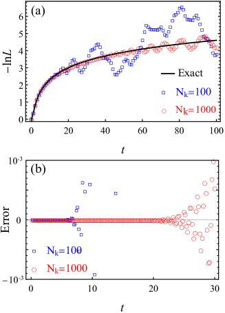
Figure 1: (Color online) A Comparative plotting of decoherence factor $L$. (a) The solid black line depicts the exact results Eq. (47). The empty blue square and red circle plot the results obtained by discretiztion approximation with the polynomial of degree $N_{k}=100,1000$ respectively. (b) the computational error is demonstrated for different $N_{k}$s.

As for the discretization of environment, it is convenient to select the weight function $w(x)=g^{2}(x)=xe^{-x}$. Replacing $H_{b}$ and $H_{\text{int}}$ by Eqs. (43) and (44), one can obtain for $-\ln L$

$$-\ln L\simeq\sum_{i=0}^{N_{k}-1}w_{i}\frac{1-\cos x_{i}t}{x_{i}^{2}}.$$ (48)

A comparison between the above expression and Eq. (47) is depicted in Fig. 1. It is evident that a higher value of $N_{k}$ leads to a more precise estimation. However, the recurrence caused by a finite $N_{k}$ can always be identified within a finite time. Therefor, to obtain the long-term behavior of $-\ln L$, a significantly large value of $N_{k}$ is required, which however can be computationally expensive.

Model II: Single-excitation open dynamics

Another exactly solvable situation is the single-excitation open dynamics. For concreteness, we explore the single-excitation dynamics in the generalized Aubry-André-Harper model (gAAH) coupled to Ohmic environment. The Hamiltonian of gAAH model is written as aah ; gAAH

$$H_{s} = \sum_{n=1}^{N_{s}}\left(c^{\dagger}_{n}c_{n+1}+c^{\dagger}_{n+1}c_{n}\right)+$$ (49)

$$+\Delta\sum_{n=1}^{N_{s}}\frac{\cos(2\pi\beta n+\phi)}{1-a\cos(2\pi\beta n+\phi)}c^{\dagger}_{n}c_{n}.$$

where $a\in[0,1)$. In order to avoid the effect of boundary, the condition $c_{N_{s}+1}=c_{1}$ is imposed in the following discussion. In the single-excitation subspace, the eigenstate of $H$ can be formulated as

$$|\psi(t)\rangle = \left(\sum_{n=1}^{N_{s}}a_{n}(t)|1\rangle_{n}\right)|0\rangle^{\otimes k}+$$ (50)

$$|0\rangle^{\otimes N_{s}}\left(\sum_{k}b_{k}(t)|1\rangle_{k}\right),$$

where $|1\rangle_{n}=c_{n}^{\dagger}|0\rangle_{n}$, $|0\rangle_{k}$ is the vacuum state of environment and $|1\rangle_{k}=b_{k}^{\dagger}|0\rangle_{k}$. Substituting Eq. (50) into Schrödinger equation and eliminating $b_{k}(t)$, one gets

$$\mathbbm{i}\frac{\partial}{\partial t}a_{n}(t) = \left[a_{n+1}(t)+a_{n-1}(t)\right]+\Delta\cos(2\pi\beta n+\phi)a_{n}(t)$$ (51)

$$- \mathbbm{i}\sum_{n=1}^{N_{s}}\int_{0}^{t}\text{d}\tau a_{n}(\tau)\int_{0}^{\infty}\text{d}\omega J(\omega)e^{-\mathbbm{i}\omega(t-\tau)},$$

where $\mathbbm{i}$ is the square root of negative 1. Eq. (51) can be solved rigorously by iteration. However, due to the memoery effect, the iteratative computation becomes so exhaustive for a long-time evoultion.

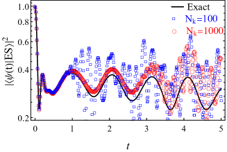
Figure 2: (Color online) A Comparative plotting of $\left|\langle\psi(t)|ES\rangle\right|^{2}$. The solid black line depicts the results obtained by solving Eq. (51). The empty blue square and red circle plot the results obtained by discretiztion approximation with the polynomial of degree $N_{k}=100,1000$ respectively. For this plot, we have chosen $N_{s}=21,\phi=\pi,\Delta=1$ and $\eta=0.1,\omega_{c}=10$.

For Ohmic spectral density Eq (3), we still choose $w(x)=g^{2}(x)=\eta\omega_{c}^{2}x^{s}e^{-x}$. Thus, $H_{b}$ or $H_{\text{int}}$ is transformed into Eqs. (43) or (44) respectively. In order to display the open dynamics, the survival probability $\left|\langle\psi(t)|ES\rangle\right|^{2}$ for the highest excited state $|ES\rangle$ of $H_{s}$, is plotted in Fig. 2. For this plot, we select $\beta=\left(\sqrt{5}-1\right)/2,a=0$, for which $H_{s}$ corresponds to the AAH model. The exact result of $\left|\langle\psi(t)|ES\rangle\right|^{2}$ is obtained by solving Eq.(50). The illustration presented in Fig. 2 demonstrates that an increase in $N_{k}$ has the potential to enhance the efficiency of estimation. However, it is important to note that the recurrence experiences significant development in a short period of time. This feature underscores the necessity to improve the discretization approximation to enable the efficient simulation of open dynamics in many-body systems.

IV Complex Gauss quadratures and Chain-Mapping in complex plane

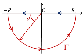
Figure 3: (Color online)The contour for the inner product defined by Eq. (52) in the complex plane.

To surmount the issue of recurrence, a viable solution is to extend the discretization approximation to the complex plane. In this section, we shall extend the discretization approximation to the complex plane by utilizing the complex Gauss quadratures.

IV.1 Complex Gauss Quadratures

In order to extend GQ to the complex plane, it is necessary to transform the definite integral in the real line into a contour integration in the complex plane. To achieve this, a semi-circle contour with a radius of $(b-a)/2$ in the lower half plane, as depicted in Fig. 3, is selected in accordance with the method presented in Refs. gautschi . This choice is crucial to obtain a unique complex polynomial with a zero point that exhibits a negative imaginary component. For the purposes of the subsequent discussion, it is assumed that $R=1$. Consequently, $z$ is defined as $e^{\mathbbm{i}\theta}$.

The inner product for complex polynomial $f(z)$ and $g(z)$ is defined as the integration along contour $\Gamma$ gautschi ,

$$\left\langle f,g\right\rangle_{\Gamma}=\int_{\Gamma}\frac{\text{d}z}{\mathbbm{i}z}w(z)f(z)g(z)=\int_{\pi}^{2\pi}\text{d}\theta w(e^{\mathbbm{i}\theta})f(e^{\mathbbm{i}\theta})g(e^{\mathbbm{i}\theta}).$$ (52)

For weight function $w(z)$, $\Re\int_{\pi}^{2\pi}\text{d}\theta w(e^{\mathbbm{i}\theta})\neq 0$ is required to guarantee that the zero point has nonvanishing imaginary part. It is notable that the inner product is defined deliberately without complex conjugation. Only by this way, the three-term recurrence relation can be constructed since $\left\langle zf,g\right\rangle_{\Gamma}=\left\langle f,zg\right\rangle_{\Gamma}$ is satisfied gautschi . As for complex polynomial $\eta_{n}(z)$ of degree $n$, the orthonormality is defined as

$$\left\langle\eta_{m},\eta_{n}\right\rangle_{\Gamma}=\int_{\pi}^{2\pi}\text{d}\theta w(e^{\mathbbm{i}\theta})\eta_{m}(e^{\mathbbm{i}\theta})\eta_{n}(e^{\mathbbm{i}\theta})=\delta_{m,n}.$$ (53)

By this relation, the following recurrence relation can be derived,

$$\sqrt{\nu_{n+1}}\eta_{n+1}(z)=\left(z-\mathbbm{i}\mu_{n}\right)\eta_{n}(z)-\sqrt{\nu_{n}}\eta_{n-1}(z),$$ (54)

where

$$\mathbbm{i}\mu_{n}=\left\langle z\eta_{n},\eta_{n}\right\rangle_{\Gamma},\nu_{n}=\frac{A^{2}_{n-1}}{A_{n}^{2}},$$ (55)

$A_{n}$ denotes the coefficient of $z^{n}$ in $\eta_{n}(z)$. Alternatively, Eq. (54) can be represented in matrix form

$$z\left(\begin{array}[]{c}\eta_{0}\\ \eta_{1}\\ \vdots\\ \eta_{n-1}\end{array}\right)=M_{c}\left(\begin{array}[]{c}\eta_{0}\\ \eta_{1}\\ \vdots\\ \eta_{n-1}\end{array}\right)+\sqrt{\nu_{n}}\left(\begin{array}[]{c}0\\ 0\\ \vdots\\ \eta_{n}\end{array}\right);$$ (68)

$$M_{c}=\left(\begin{array}[]{cccc}\mathbbm{i}\mu_{0}&\sqrt{\nu_{1}}&0&\cdots\\ \sqrt{\nu_{1}}&\mathbbm{i}\mu_{1}&\ddots&0\\ 0&\ddots&\ddots&\sqrt{\nu_{N_{k}-1}}\\ 0&\cdots&\sqrt{\nu_{N_{k}-1}}&\mathbbm{i}\mu_{N_{k}-1}\end{array}\right).$$ (73)

Thus, the zero points $z_{i}$ and its weight $w_{i}$ for $\eta_{n}(z)$ can be obtained by solving eigenvalues and corresponding eigenfunctions of $M_{c}$. Noting that $M_{c}$ is complex symmetric, the right and left eigenfunctions have relation $|n\rangle_{R}=\left(|n\rangle_{L}\right)^{*}$. Similar to the real situation, one gets

$$w_{i}=\left[q^{(i)}_{0}\right]^{2}\int_{\pi}^{2\pi}\text{d}\theta w(e^{\mathbbm{i}\theta}).$$ (74)

where $q^{(i)}_{0}$ denotes the first element of right eigenfunction for zero point $z_{i}$. It can be proved that $z_{i}$ is confined in the region bounded by $\Gamma$ and $x$-axis wilf . With these results, the following relation can be constructed

$$\int_{\Gamma}\frac{\text{d}z}{\mathbbm{i}z}w(z)f(z)\simeq\sum_{i}w_{i}f(z_{i}),$$ (75)

that is the generalization of Theorem 1 into the complex plane gautschi .

Finally, it should be pointed out that the complex orthonormalized polynomial $\eta_{n}(z)$ is relevant significantly to its real counterpart $\pi_{n}(x)$. The exact connection between $\eta_{n}(z)$ and $\pi_{n}(x)$ has been constructed in Refs. gautschi . By this relevance, $\eta_{n}(z)$ can also be obtained directly by $\pi_{n}(x)$.

IV.2 Mapping to the chain form

For analytical function $f(z)$ in the complex plane, one has by Cauchy theorem,

$$\int_{C}\text{d}zf(z)=\int_{\Gamma}\text{d}zf(z)-\int_{-R}^{R}\text{d}xf(x)=0$$

$$\therefore\int_{-R}^{R}\text{d}xf(x)=\int_{\Gamma}\text{d}zf(z).$$ (76)

where $C$ denotes close path depicted by the arrows in Fig. 3. With the requirement that both $h(z)$ and $g(z)$ are analytical in the complex plan, one can replace $\int_{-R}^{R}\text{d}x$ by $\int_{\Gamma}\text{d}z$. Correspondingly, $b_{x}^{\dagger},b_{x}$ is replaced by $b_{z}^{\dagger},b_{z}$, and the commutative relation becomes $\left[b_{z},b^{\dagger}_{z^{\prime}}\right]=\delta\left(z-z^{\prime}\right)$. Then the question is how to discretize the path integral along $\Gamma$.

Similar to the approach in section IIIB, let first introduce the transformation

$$d_{n} = \int_{\Gamma}\text{d}z\sqrt{\frac{w(z)}{\mathbbm{i}z}}\eta_{n}(z)b_{z}$$

$$d_{n}^{{\ddagger}} = \int_{\Gamma}\text{d}z\sqrt{\frac{w(z)}{\mathbbm{i}z}}\eta_{n}(z)b_{z}^{\dagger}$$ (77)

and the inverse

$$b_{z} = \sqrt{\frac{w(z)}{\mathbbm{i}z}}\sum_{n=0}^{N_{k}-1}\eta_{n}(z)d_{n}$$

$$b_{z}^{\dagger} = \sqrt{\frac{w(z)}{\mathbbm{i}z}}\sum_{n=0}^{N_{k}-1}\eta_{n}(z)d_{n}^{{\ddagger}}.$$ (78)

It should be stressed that $d_{n}^{{\ddagger}}$ is not the Hermitian conjugation of $d_{n}$, due to the inner product defined in Eq. (52). It is easy to prove

$$\left[d_{n},d_{m}^{{\ddagger}}\right] = \iint\text{d}z\text{d}z^{\prime}\sqrt{\frac{w(z)w(z^{\prime})}{\mathbbm{i}^{2}zz^{\prime}}}\eta_{m}(z)\eta_{n}(z^{\prime})\left[b_{z},b_{z^{\prime}}^{\dagger}\right]$$ (79)

$$= \int\text{d}z\frac{w(z)}{\mathbbm{i}z}\eta_{m}(z)\eta_{n}(z)=\delta_{m,n}.$$

However the transformation Eqs.(IV.2) is not unitary for finite $N_{k}$, which is responsible for the computational errors.

Substituting Eqs. (IV.2) into $H_{b}$, one obtains

$$H_{b}=\omega_{c}\sum_{i,j}d_{i}^{{\ddagger}}d_{j}\int_{\Gamma}\text{d}z\frac{w(z)}{\mathbbm{i}z}z\eta_{i}(z)\eta_{j}(z).$$ (80)

Replacing $z\eta_{i}(z)$ by solving Eq. (54) and applying Eq. (53), one gets

$$H_{b} = \omega_{c}\left(\cdots,d_{m}^{\dagger},\cdots\right)M_{c}\left(\begin{array}[]{c}\vdots\\ d_{n}\\ \vdots\end{array}\right),$$ (84)

in which $M_{c}$ is given in Eq. (68). Resultantly, the eigenvalue of $M_{c}$ correspond to the discrete mode in environment, which is complex due to the nonhermiticity of $M_{c}$. Defining the new mode operator

$$\widetilde{d}_{i} = \sqrt{w_{i}}\sum_{n=0}^{N_{k}-1}\eta_{n}(z_{i})d_{n},$$

$$\widetilde{d}_{i}^{\ddagger} = \sqrt{w_{i}}\sum_{n=0}^{N_{k}-1}\eta_{n}(z_{i})d_{n}^{\ddagger},$$ (85)

$H_{b}$ can be diagonalized,

$$H_{b}=\sum_{i=0}^{N_{k}-1}z_{i}\widetilde{d}_{i}^{\ddagger}\widetilde{d}_{i}.$$ (86)

As for $H_{\text{int}}$, one gets

$$H_{\text{int}}=\sum_{n=1}^{N_{s}}\sum_{i=0}^{N_{k}-1}\int_{\Gamma}\text{d}z\sqrt{\frac{w(z)}{\mathbbm{i}z}}\eta_{i}(z)\left[g(z)c^{\dagger}_{n}d_{i}+g^{*}(z)d_{i}^{\ddagger}c_{n}\right],$$ (87)

in which $g(z)$ is the generalization of $g(x)$ into the complex plane.

IV.3 Simplification of $H_{\text{int}}$

In order to simplify Eq. (87), one has to deal with the integration in Eq.(87). The integration $\int_{\Gamma}\text{d}z\sqrt{\frac{w(z)}{\mathbbm{i}z}}\eta_{i}(z)g(z)$ appears to be evaluated numerically only if $\eta_{i}(z)$ is known. However, empirical analysis has revealed that this methodology is not feasible. Instead, the correct way is to approximate the integration according to Eq. (75) as

$$\int_{\Gamma}\text{d}z\sqrt{\frac{w(z)}{\mathbbm{i}z}}\eta_{i}(z)g(z) = \int_{\Gamma}\text{d}z\frac{w(z)}{\mathbbm{i}z}\sqrt{\frac{\mathbbm{i}z}{w(z)}}\eta_{i}(z)g(z)$$ (88)

$$\simeq \sum_{j=0}^{N_{k}-1}\sqrt{\frac{\mathbbm{i}z_{j}}{w(z_{j})}}w_{j}\eta_{i}(z_{j})g(z_{j}).$$

Then, the first term in Eq.(87) is transformed into

$$\sum_{n=1}^{N_{s}}\sum_{i,j=0}^{N_{k}-1}\sqrt{\frac{\mathbbm{i}z_{j}}{w(z_{j})}}w_{j}\eta_{i}(z_{j})g(z_{j})c^{\dagger}_{n}d_{i}$$ (89)

$$= \sum_{n}^{N_{s}}\sum_{j=0}^{N_{k}-1}\sqrt{\frac{\mathbbm{i}z_{j}}{w(z_{j})}}\sqrt{w_{j}}g(z_{j})c^{\dagger}_{n}\widetilde{d}_{j}$$

where the second equality comes from Eq. (IV.2).

However, the method presented in Eq. (88) for evaluating $\int_{\Gamma}\text{d}z\sqrt{\frac{w(z)}{\mathbbm{i}z}}\eta_{i}(z)g^{*}(z)$ encounters difficulties.This is due to the fact that $g^{*}(z)$ can be written as $g(z^{*})$ based on the definition of $g(x)$ in Eq. (4), which prevents proper evaluation. In another point, the total number of excitation in the system and environment remains constant during evolution, leading to the replacement of the second term in Eq. (87) with the complex conjugate of the first term. Accordingly, $H_{\text{int}}$ can be approximated as

$$H_{\text{int}} \simeq \sum_{n}^{N_{s}}\sum_{j=0}^{N_{k}-1}\left[\sqrt{\frac{\mathbbm{i}z_{j}}{w(z_{j})}}\sqrt{w_{j}}g(z_{j})c^{\dagger}_{n}\widetilde{d}_{j}+\text{h. c. }\right]$$ (90)

$$= \sum_{n}^{N_{s}}\sum_{j=0}^{N_{k}-1}\left(\mathbbm{g}_{j}c^{\dagger}_{n}\widetilde{d}_{j}+\text{h. c. }\right)$$

where $\mathbbm{g}_{j}=\sqrt{\frac{\mathbbm{i}z_{j}}{w(z_{j})}}\sqrt{w_{j}}g(z_{j})$. This point can be verified by two illustrations in the subsection IV.5.

IV.4 Evaluating the full dynamics

To ensure that the physical requirement is met, it is important to select an appropriate value for $R$ during the actual calculation. In the case of an Ohmic environment, where $x$ falls within the range of $\left[0,\infty\right)$ in $J(x)$, it is necessary to perform a translation of $z_{j}$ to $R(1+z_{j})$. This ensures that the real part of $R(1+z_{j})$ corresponds to the value of $x$. Under this translation, one has

$$z_{i} \rightarrow R(1+z_{j})$$

$$\mathbbm{g}_{j} \rightarrow \sqrt{\frac{\mathbbm{i}Rz_{j}}{w\left[R(1+z_{j})\right]}}\sqrt{w_{j}}g\left[R(1+z_{j})\right],$$

The $\mathbbm{i}Rz_{j}$ is a result of the requirement that $\int_{\Gamma}\frac{\text{d}z}{\mathbbm{i}z}=\int_{\pi}^{2\pi}\text{d}\theta$ must be preserved under the translation. The precision of numerical evaluation can be improved by increasing the value of $R$ since it determines the upper bound of integration.

Eventually, a non-Hermitian effective Hamiltonian, labelled by $H_{\text{eff}}$, can be obtained, which is a function of $R$. The eigenfunctions of $H_{\text{eff}}$ satisfy the biorthonormality rotter09 ,

$${{}_{L}\langle m|n\rangle_{R}}=\delta_{m,n},$$ (91)

where $|n\rangle_{R}$ denotes the right eigenfunction of $H_{\text{eff}}$ with eigenvalue $\mathbbm{E}_{n}$, and $|n\rangle_{L}$ denotes the left eigenfunction with eigenvalue $\mathbbm{E}^{*}_{n}$. By solving the Schrödinger equation, the total state $|\psi(t)\rangle$ at any time $t$ can be expressed as

$$|\psi(t)\rangle=\sum_{n}e^{-\mathbbm{iE}_{n}t}|n\rangle_{R}{{}_{L}\langle n|\psi(0)\rangle}.$$ (92)

With these technique preparations, we are ready to reexamine the open dynamics in dephasing model and gAAH model by the current method.

IV.5 Illustrations

To ensure efficient simulation, it is essential to carefully select $w(z)$. Our findings indicate that using $w(z)/\mathbbm{i}z=\eta\omega^{2}_{c}z^{s}e^{-z}$ is not a suitable choice, as it can cause $M_{c}$ to become real symmetric. This, in turn, results in real eigenvalues and dynamics that are identical to those in the real case. To overcome this limitation and obtain complex $z_{i}$, we use $w(z)=1$. This modification leads to a significant improvement in the simulation, as discussed in the following.

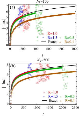
Figure 4: (Color online) The plots for the modulus of $-\ln L$ defined in Eq. (IV.5) with different $R$ and $N_{k}$. For the plots, $\eta=\omega_{c}=1$ is chosen for simplicity. The solid black line corresponds to the exact result Eq. (47).

Model I: Dephasing

By Eq. (46), one gets

$$-\ln L= \sum_{j} \left|\sqrt{\frac{\mathbbm{i}Rz_{j}}{w\left[R(1+z_{j})\right]}}\sqrt{w_{j}}g\left[R(1+z_{j})\right]\right|^{2}$$

$$\times\frac{1-\cos R(1+z_{j})t}{R^{2}(1+z_{j})^{2}}$$

Fig. 4 illustrates the modulus of $-\ln L$, which indicates a marked improvement in simulation due to the implementation of complex discretization approximation. The accuracy and efficiency of evaluation are influenced by both $N_{k}$ and $R$. The maximum time for which $-\ln L$ can be evaluated rigorously is determined by increasing $N_{k}$, while the precision of computation is determined by $R$. Thus, achieving the desired efficiency and precision in computation requires a balanced selection of both $N_{k}$ and $R$.

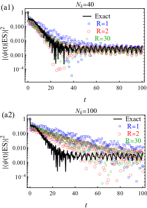
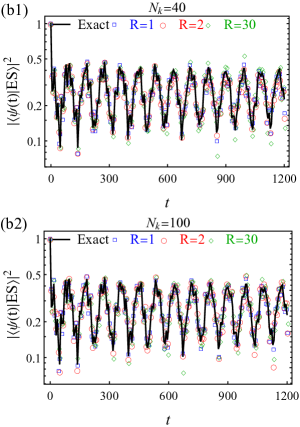
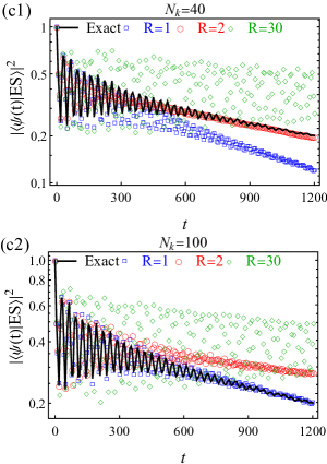
Figure 5: (Color online) The plots for the survival probability $\left|\langle\psi(t)|ES\rangle\right|^{2}$ vs. $R$ and $N_{k}$. The solid black line characterizes the exact result by solving Eq. (51). Panel (a1) and (a2) are plotted for $\Delta=1$. Panel (b1) and (b2) is for $\Delta=2.5$; Panel (c1) and (c2) is for $\Delta=6$. For all plots, $N_{s}=21,\beta=\left(\sqrt{5}-1\right)/2,a=0,\phi=\pi,\eta=0.1$, and $\omega_{c}=10$ are chosen.

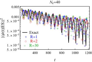
Figure 6: (Color online) The plots of the long-time behavior for the evaluation shown in Fig. 5 (a1).

Model II: Singel-excitation subspace

The situation regarding single-excitation dynamics in the gAAH model coupled to an Ohmic environment is complex. The survival probability, represented by $\left|\langle\psi(t)|ES\rangle\right|^{2}$, is calculated using the complex discretization approximation for various values of $R$ and $N_{k}$. The results showed a clear dependence on the system’s state. For instance, when the system was in a delocalized phase with $\Delta=1$, the accuracy of the calculation was higher with $N_{k}=40$ than with $N_{k}=100$,, as shown by Figs. 5 (a1) and (a2). Additionally, the further calculation indicates that $R=2,N_{k}=40$ would appear to be the preferred value for accuracy, and deviation from this value may decrease precision. This trend persisted over long-time evolution as show in Fig. 6. It should be noted that the accuracy of the computation was lower for $t<\sim 20$.

When $\Delta=2.5$, where the system is known to be in localized phase aah . As shown by Figs. 5 (b1) and (b2), the calculated result shows good consistency to the exact one for both $N_{k}=40$ and $N_{k}=100$. Moreover, it is found that the choice of $R$ could not significantly affect the calculation, so a value of $R=2$ is preferred. However, for $\Delta=6$, where the system is strongly localized, a careful selection of $N_{k}$ and $R$ is necessary to accurately evaluate $\left|\langle\psi(t)|ES\rangle\right|^{2}$. In Figs. 5 (c1) and (c2), it is shown that a value of $R=2$ is chosen for $N_{k}=40$, while a value of $R=1$ is chosen for $N_{k}=100$ in order to obtain precise results.

The complex discretization method has been shown to be helpful in improving computational efficiency, but its effectiveness depends on the system properties and coupling to the environment. For the dephasing model, the decoherence factor can only be accurately determined by increasing both $N_{k}$ and $R$. However, for the single-excitation dynamics in the open gAAH model, a preferred choice of $N_{k}=40$ and $R=2$ is sufficient, as shown in Fig. 5. This difference can be attributed to the varying coupling between the system and environment, as described by $H_{\text{int}}$. In the dephasing model, there is no exchange of energy or particles between the system and environment, with the latter acting as a measurer to detect energy levels in the system. Increasing $N_{k}$ and $R$ in this case improves the precision of the measurement. In contrast, the single-excitation dynamics in the gAAH model is the result of energy transport between the system and environment. The dissipative dynamics in the system can be attributed to resonate states, which correspond to the eigenfunctions of a non-Hermitian effective Hamiltonian for the system rotter09 . The existence of these states implies that dissipation in the system is primarily due to coupling to separated modes in the environment. The preferred choice of $N_{k}$ and $R$ in this case reflects the presence of resonate states.

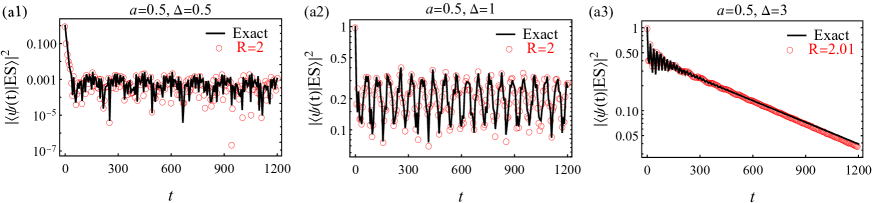
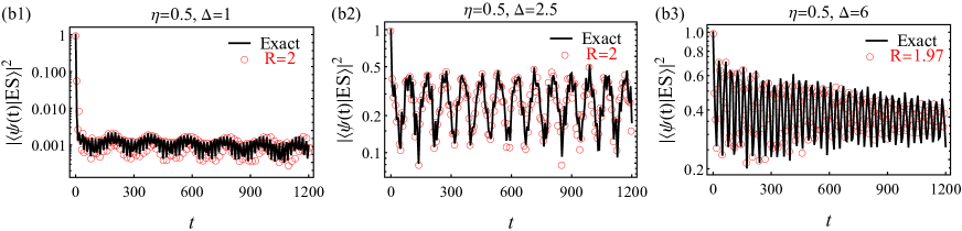
Figure 7: (Color online) The plots for $\left|\langle\psi(t)|ES\rangle\right|^{2}$ when $a=0.5$ or $\eta=0.5$ individually. $N_{s}=21,\beta=\left(\sqrt{5}-1\right)/2,\phi=\pi$, and $\omega_{c}=10$ have been chosen for all plots. As for panels (a1)-(a3), $a=0.5$ and $\eta=0.1$ are chosen. For panels (b1)-(b3), $a=0$ and $\eta=0.5$ are chosen.

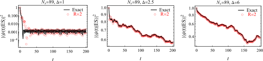
Figure 8: (Color online) The plots of $\left|\langle\psi(t)|ES\rangle\right|^{2}$ for different $\Delta$ when $N_{s}=89$ is chosen. The other parameters are the same as those in Figs. 5.

IV.6 Relevance to the properties of $H_{s}$

In this subsection, we aim to demonstrate that the values of $N_{k}=40$ and $R=2$ are suitable for simulating open single-excitation dynamics in the gAAH model. To do this, we vary the parameters $a$, $\eta$, and $N_{s}$. Specifically, we plot $\left|\langle\psi(t)|ES\rangle\right|^{2}$ for different values of $a$ and $\eta$ in Fig. 7. When $a=0.5$, the localization-delocalization transition disappears and a mobility edge (ME) can occurgAAH . Figs. 7 (a1)-(a3) show the influence of the ME for different values of $\Delta$, where $|ES\rangle$ is extended, weakly localized, or deeply localized, respectively. We find that the choice of $N_{k}=40$ and $R=2$ provides accurate results for $\Delta=0.5$ and $1$, but a slight variation of $R$ is needed to improve the calculation for $\Delta=3$. Similar observations are made for $\eta=0.5$, as shown in Figs. 7 (b1)-(b3).

In Fig. 8, we explore the effect of the number of sites in the system by fixing $N_{s}=89$. The computation of Eq. (51) becomes exhaustive in this scenario. Hence, we restrict the graph to $t=200$. Despite this limitation, our assessment continues to deliver reliable long-term forecasts that align with the precise computation.

V single-excitation open dynamic in gAAH model: revisited

In this section, the robustness of delocalization-localization transition and the mobility edge in gAAH model against dissipation is investigated by the complex discretization approximation. For $a=0$, the delocalization-localization phase transition can occur when $\Delta=2$. While for $a\in\left(0,1\right)$ the mobility edge (ME) $E_{c}$ can be decided by the relation

$$aE_{c}=\text{sign}\left(\lambda\right)\left(2\left|\lambda\right|-\left|\Delta\right|\right).$$ (93)

Then the energy levels $E_{n}$ in the gAAH model are extended when $E_{n}<E_{c}$ or localized when $E_{n}>E_{c}$. The exact approach to determining the robustness of the transition and ME requires solving Eq. (51) for all eigenfunctions, which is computationally exhaustive. However, the complex discretization approximation makes it simple to solve the eigenvalues and eigenfunctions for $H_{\text{eff}}$ and determine the state evolution for arbitrary $t$ using Eq. (92).

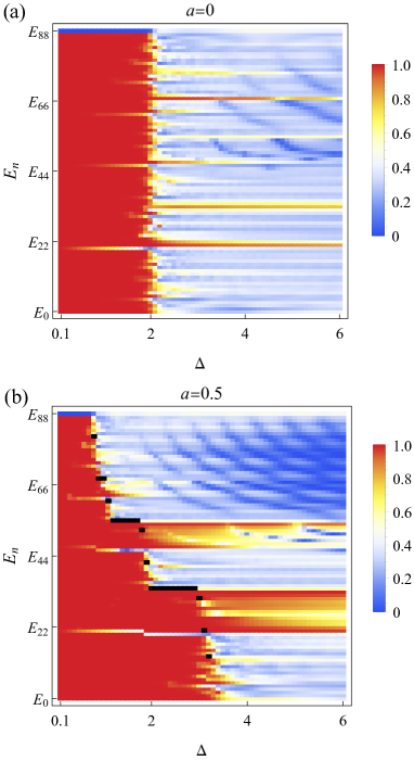
Figure 9: (Color online) The plots of averaged survival probability defined in Eq. (94) for all $|E_{n}\rangle$s in Eq. (49) with $N_{s}=89$. For the plots, we have chosen $N_{k}=40,R=2$, as well as $\beta=\left(\sqrt{5}-1\right)/2,\phi=\pi,\eta=0.1$, and $\omega_{c}=10$. In panel (b), the black solid rectangles denote the highest $E_{n}$ smaller than $E_{c}$.

To reveal the resilience of the phase transition and ME, the averaged survival probability (ASP), defined as

$$\text{ASP}=\frac{\int_{t_{0}}^{t}\text{d}t\left|\langle E_{n}|e^{-\mathbbm{i}H_{\text{eff}}t}|E_{n}\rangle\right|^{2}}{t-t_{0}},$$ (94)

is calculated for all $|E_{n}\rangle(n=0,1,\cdots,N_{s}-1)$. The efficiency of evaluation is confirmed for the chosen values of $t_{0}=100$ and $t=1000$. As shown in Fig. 9, ASP can display distinct behavior depending on the value of $a$.

When $a=0$, it is evident that the diagram is divided into two regions by $\Delta=2$ and ASP displays distinct behavior, as shown in Fig. 9(a). Contrary to intuition, the states that are more extended show a higher value of ASP (close to 1) when $\Delta<2$, while the localized states have a lower value (close to 0.5) when $\Delta>2$. This is attributed to the single-particle property of localization in gAAH model. The excitation behaves like a single particle in the localized phase, making it easier to be absorbed by the environment. However, the correlation induced by hopping in the extended states protects them against dissipation. The highest excited state, labeled as $|E_{88}\rangle$, exhibits an exceptional behavior where ASP tends to be vanishing when $\Delta<2$ and shows a finite value when $\Delta>2$. The reason for this behavior is not yet understood. Nonetheless, the delocalization-localization transition in the gAAH model can still be observed under dissipation.

When $a=0.5$, the diagram becomes fragmental due to the presence of ME, as shown in Fig. 9 (b). For clarity, the highest level with energy $E_{n}$ below the critical energy $E_{c}$ is highlighted in a black-solid rectangle (for $\Delta>\sim 3.5$, all $E_{n}$ behave localized in this case). In most cases, ASP is smaller for $E_{n}$ above $E_{c}$ than for those below it. However, there are certain energy levels, such as those between approximately $\sim 22<n<\sim 33$ and $\sim 44<n<\sim 50$, where ASP does not degrade rapidly even when the system becomes strongly localized. This suggests that extended and localized state may become mixed, and MEs are needed to define the transition between them. For example, the stable ASP for energy levels between approximately $\sim 22<n<\sim 33$ suggests the introduction of two additional critical energies, $E_{22}$ and $E_{33}$, to characterize distinct energy regions.

VI Conclusions and discussion

In conclusion, this paper introduces a generalized approach for approximating the environment in continuum using complex gauss quadratures in the complex plane. The method is applied to investigate the open dynamics in two solvable models, namely the dephasing model and single-excitation open dynamics in the gAAH model. Compared to the real counterpart, the complex generalization significantly enhances computational efficiency. Additionally, the paper explores the robustness of the localization-delocalization transition and the mobility edge against dissipation using the complex discretization approximation.

The complex discretization approximation offers a significant advantage in compressing the recurrence in dynamics, thanks to the discrete complex modes with negative imaginary part in the environment. This results in a non-Hermitian effective Hamiltonian that accurately reflects the dissipative dynamics in the system. However, determining the appropriate values of $R$ and $N_{k}$ is crucial for accuracy, which can be achieved by comparing the approximation with the exact evaluation, e.g. obtained through single-excitation open dynamics.

There is uncertainty regarding whether the complex discretization approximation is suitable for simulating the open dynamics in interacting many-body systems. While it is expected that our method can accurately simulate open dynamics despite entangled single-particle states due to interactions, it is challenging to precisely tackle the interacting dynamics in many-body systems. Additionally, it is difficult to determine the exact dynamics in open interacting many-body systems, which is necessary to verify the validity of the complex discretization approximation. We will present further research on this topic in the future. Another question that arises is how to factor in the impact of temperature in the surrounding environment when making the discretization approximation. One potential solution involves adjusting the spectral function to account for temperature, which would result in temperature-dependent discrete modes in the environment as well as a varying coupling strength between the system and environment finitetemperature . As a result, the issue of finite temperature can be transformed into a zero temperature scenario, allowing for easier application of the current method in addressing open dynamics in the system. Further exploration of this topic will be undertaken in future research.

Finally, it should be stressed that the complex discretization approximation and the method of pseudomode are two fundamentally different approaches. In the pseudomode method pseudomode , the environment is discretized based on the complex poles of the spectral function $J(x)$, resulting in an enlarged open system with discrete modes. The dynamics of this system is captured by the Markovian Lindblad master equation. However, in the current method, the spectral function must be continuous in the lower half complex plane, and there is no need for the introduction of additional Markovian processes. The effective Hamiltonian obtained through this method can accurately describe the open dynamics of the system.

DATA AVAILABILITY

The data for the calculation in this study are available from the correspond author upon request. Correspondence and request for materials should be addressed to H. T. Cui.

AUTHOR CONTRIBUTIONS

H.T.C. conceived the idea of this paper. H. T. C., Y. A. Y. and M. Q. carried out the theoretical deduction and numerical computation. X. X. Y. supervised the project. All authors contributed to the preparation of manuscript.

References

- (1) H. P. Breuer, F. Petruccione, The Theory of Open Quantum Systems, Oxford University Press (2002).
- (2) I. M. Georgescu, S. Ashhab, Franco Nori, Qauntum Simulation, Rev. Mod. Phys. 86, 154 (2014); M. Gong, et.al., Quantum walks on a programmable two-dimensional 62-qubit superconducting processor, Science, 372, 948-952 (2021); Q. Zhu, et.al., Quantum computational advantage via 60-qubit 24-cycle random circuit sampling, Science Bulletin, 67(3), 240-245 (2022).
- (3) A. F. Kockum, A. Miranowicz, S. De Liberato, S. Savasta and F. Nori, Nat. Rev. Phys. 1, 19-40 (2019); P. Forn-Dìaz, L. Lamata, E. Rico, J. Kono, and E. Solano, Rev. Mod. Phys. 91, 025005.
- (4) A. W. Chin, S. F. Huelga and M. B. Plenio, Coherence and decoherence in biologicalsystems: principles of noise-assisted transportand the origin of long-lived coherences, Phil. R. Soc. A, 370, 3638–3657 (2012); A. Ivanov, H. P. Breuer, Phys. Rev. A 92, 032113 (2015); F. Caycedo-Soler, A. Mattioni, J. Lim, T. Renger, S. F. Huelga, M. B. Plenio, Exact simulation of pigment-protein complexes unveils vibronic renormalization of electronic parameters in ultrafast spectroscopy, Nat. Commun. 13, 2912 (2022).
- (5) F. Binder, L. A. Correa, C. Gogolin, J. Anders, and G. Adesso, Thermodynamics in the Quantum regime, Springer, Cham, Switzerland (2018); G. T. Landi and M. Paternostro, Irreversible entropy production: From classical to quantum, Rev. Mod. Phys. 93, 035008 (2021).
- (6) E. Zerah-Harush and Y. Dubi, Effect of disorder and interactions in environment assited quantum transport, Phys. Rev. Reseach, 2, 023294 (2020); N. C. Cháves, F. Mattiotti, J. A. Méndez-Bermúdez, F. Borgonovi, and G. Luca Celardo, Disorder-enhanced, and disorder-independent transport with long-range hopping: application to molecular chains in optical cavities, Phys. Rev. Lett. 126, 153201 (2021); D. Dwiputra, and F. P. Zen, Enviornment-assited quantum transport and mobility edges, Phys. Rev. A 104, 022205 (2021); H. T. Cui, M. Qin, L. Tang, H. Z. Shen, and X. X. Yi, Localization-enhanced dissipation in a generalized Aubry-André-Harper model coupled with Ohmic baths, Phys. Lett. A 448, 128314 (2022).
- (7) I. de Vega, D. Alonso, Dynamics of non-Markovian open quantum systems, Rev. Mod. Phys. 89, 015001 (2017).
- (8) S. Nakajima, On Quantum Theory of Transport Phenomena: Steady Diffusion, Prog. Theor. Phys. 20, 948 (1958); R. Zwanzig, Ensemble Method in the Theory of Irreversibility, J. chem. Phys. 33, 1338 (1960).
- (9) F. Shibata, Y. Takahashi, and N. Hashitsume, A generalized stochastic Liouville equation. NonMarkovian versus memoryless master equations, J. Stat. Phys. 17, 171 (1977); S. Chaturvedi and F. Shibata, Time- convolutionless projection operator formalism for elimination of fast variables. Applications to Brownian motion, Z. Phys. B 35, 297 (1979); F. Shibata and T. Arimitsu, Expansion Formulas in Nonequilibrium Statistical Mechanics, J. Phys. Soc. Jpn. 49, 891 (1980).
- (10) J. Cao, L. W. Ungar, and G. A. Voth, A novel method for simulating quantum dissipative systems. J. Chem. Phys. 104, 4189 (1996); Y.-A. Yan, J.-S. Shao, Stochastic description of quantum Brownian dynamics, Front. Phys. 11, 110309 (2016).
- (11) Y. Tanimura and R. Kubo, Time Evolution of a Quantum System in Contact with a Nearly Gaussian-Markoffian Noise Bath, J. Phys. Soc. Jpn. 58, 101(1989); Y.-A. Yan, F. Yang, Y. Liu, and J.-S. Shao, Hierarchical approach based on stochastic decoupling to dissipative systems, Chem. Phys. Lett. 395, 216-221 (2004).
- (12) N. Makri and D. E. Makarov, Tensor propagator for iterative quantum time evolution of reduced density matrices. I. theory, J. Chem. Phys. 102, 4600 (1995); ibid., Tensor propagator for iterative quantum time evolution of reduced density matrices. II. Numerical methodology,J. Chem. Phys. 102, 4611 (1995).
- (13) R. Rosenbach, J. Cerrillo, S. F. Huelga, J. Cao, and M. B. Plenio, Efficient simulation of non-Markovian system-environment interaction, New J. Phys. 18, 023035 (2016); A. Strathearn, P. Kirton, D. Kilda, J. Keeling, and B. W. Lovett, Efficient non-Markovian quantum dynamics using time-evolving matrix product operators, Nat. Commun. 9, 3322 (2018);
- (14) A. W. Chin, Á. Rivas, S. F. Huelga, and M. B. Plenio, Exact mapping between system-reservior quantum models and semi-infinite discrete chains using orthogonal polynomials, J. Math. Phys. 51, 092109 (2010); M. P. Woods, R. Groux, A. W. Chin, S. F. Huelga, and M. B. Plenio, Mappings of open quantum systems onto chain respresentations and Markovian embeddings. J. Math. Phys. 55, 032101 (2014).
- (15) R. Trivedi, D. Malz, and J. I. Cirac, Convergence guarantees for discrete mode approximantion to non-Markovian quantum baths, Phys. Rev. Lett. 127, 250404 (2021).
- (16) R. S. Burkey, C. D. Cantrell, Discretization in the quasi-continuum, J. Opt. Soc. Am. B 1, 169-175 (1984); A. K. Kazansky, Precise anlaysis of resonance decay law in atomic physics, J. Phys. B: At. Mol. Opt. Phys. 30, 1404-1410 (1997); N. Shenvi, J. R. Schmidt, S. T. Edwards, and J. C. Tully, Efficient decretization of the continuum through complex contour deformation, Phys. Rev. A 78, 022502 (2008).
- (17) S. Aubry and G. André, Analyticity Breaking and Anderson Localization in Incommensurate Lattices, Ann. Isr. Phys. Soc. 3, 33 (1980); P. G. Haper, Single Band Motion of Conduction Electrons in a Uniform Magnetic Field, Proc. Phys. Soc. London Sect. A 68, 874 (1955).
- (18) S. Ganeshan, J. H. Pixley, and S. Das Sarma, Nearest neighbor tight binding models with an exact mobility edge in one dimension, Phys. Rev. Lett. 114, 146601 (2015).
- (19) Herbert S. Wilf, Mathematics for the Physcial Sciences, Dover Publication, inc. (New York, 1962).
- (20) W. Gautshci, G. V. Milovanović, Polynomials orthognal on the Semicircle, J. Approx. Theo. 46, 230-250 (1986); W. Gautschi, H. J. Landau, and G. V. Milovanović, Polynomials orthognal on the Semicircle II, Constr. Approx. 3, 389-404 (1987).
- (21) H. T. Cui, M. Qin, L. Tang, H. Z. Shen, and X. X. Yi, Localization-enhanced dissipation in a generalized Aubry-André-Harper model coupled with Ohmic baths, Phys. Lett. A 448, 128314 (2022).
- (22) I. Rotter, A non-Hermitian Hamilton operator and the physics of open quantum systems, J. Phys. A: Math. Theor. 42, 153001 (2009).
- (23) D. Tamascelli, A. Smirne, J. Lim, S. F. Huelga, and M. B. Plenio, Efficient simulation of finite-temperature open quantum systems, Phys. Rev. Lett. 123, 090402 (2019); A. J. Dunnet, A. W. Chin, Simulating quantum vibronic dynamics at fininte temperature with many-body wave functions at 0K, Front. Chem. 8, 2296 (2021); K. T. Liu, D. N. Beratan, and P. Zhang, Improving the efficiency of open-quantum-system simulatations using matrix product state in the interactiion picutre, Phys. Rev. A 105, 032406 (2022).
- (24) B. M. Garraway, Nonperturbative decay of an atomic system in a cavity, Phys. Rev. A 55, 2290-2303 (1996); D. Tamascelli, A. Smirne, S. F. Huelga, and M. B. Plenio, Phys. Rev. Lett. 120, 030402 (2018); N. Lambert, S. Ahmed, M. Cirio, and F. Nori, Nat. Commun. 10, 3721 (2019); S. Xu, H. Z. Shen, X. X. Yi, and W. Wang, Readout of the spectral density of an environment from the dynamics of an open system , Phys. Rev. A 100, 032108 (2019); G. Pleasance, B. M. Garraway, and F. Petruccione, Generalized theory of pseudomodes for exace description of non-Markovian quantum processes, Phys. Rev. Res. 2, 043058 (2020); G. Pleasance, F. Petruccione, Pseudomode desciption of general open quantum system dynamics: non-perturbative master equation for the spin-boson model, arXiv: 2108.05755 [quant-ph] (2021).