Predictive Experience Replay for Continual
Visual Control and Forecasting

Abstract

Learning physical dynamics in a series of non-stationary environments is a challenging but essential task for model-based reinforcement learning (MBRL) with visual inputs. It requires the agent to consistently adapt to novel tasks without forgetting previous knowledge. In this paper, we present a new continual learning approach for visual dynamics modeling and explore its efficacy in visual control and forecasting. The key assumption is that an ideal world model can provide a non-forgetting environment simulator, which enables the agent to optimize the policy in a multi-task learning manner based on the imagined trajectories from the world model. To this end, we first propose the mixture world model that learns task-specific dynamics priors with a mixture of Gaussians, and then introduce a new training strategy to overcome catastrophic forgetting, which we call predictive experience replay. Finally, we extend these methods to continual RL and further address the value estimation problems with the exploratory-conservative behavior learning approach. Our model remarkably outperforms the naïve combinations of existing continual learning and visual RL algorithms on DeepMind Control and Meta-World benchmarks with continual visual control tasks. It is also shown to effectively alleviate the forgetting of spatiotemporal dynamics in video prediction datasets with evolving domains.

1 Introduction

World models, in form of neural networks, learn to simulate the physical processes in a given environment through visual observation and interaction. They greatly benefit real-world applications including spatiotemporal data forecasting [1, 2, 3] and robotic reinforcement learning (RL) with image inputs [4, 5, 6]. A typical learning setup is to operate the model in a stationary environment with relatively fixed physical dynamics. However, the assumption of stationarity does not always hold in more realistic scenarios, such as in the settings of continual learning, where the learning system needs to handle different tasks in a streaming manner. For example, in robotics (see Fig. 1), an agent may experience different tasks with various spatiotemporal patterns sequentially throughout its life cycle. Therefore, it needs to constantly adapt to new tasks without forgetting previous knowledge, which is known as the problem of catastrophic forgetting.

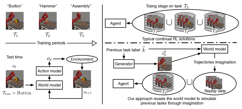
Figure 1: Left: The new problems of continual visual control and forecasting. Top Right: Existing continual RL solutions typically retain large amounts of previous data in a replay buffer to train model-free RL models. Bottom Right: We present a pilot work of MBRL in continual visual control. The key assumption is that a “non-forgetting” world model can be a cornerstone for mitigating the catastrophic forgetting of RL policies.

In this paper, we make an early study of continual learning in the realm of visual control and forecasting. Unlike the previous efforts to integrate standard solutions for catastrophic forgetting into model-free RL methods [7, 8, 9, 10], in our setup with high-dimensional video inputs, it is impractical to retain a large data buffer for each previous task. Instead, we suggest that the key challenge is rooted in combating the distribution shift in dynamics modeling. The basic assumption of our approach is that an ideal world model can be viewed as a natural remedy against catastrophic forgetting in continual RL scenarios, because it can replay the previous environments through “imagination”, allowing multi-task policy optimization.

Therefore, the key is to obtain a “lifelong” world model across sequential tasks with a long-lasting memory for non-stationary spatiotemporal dynamics. To this end, we need to particularly consider a triplet of distribution shift, including covariate shift in input data space [11, 12, 13, 14, 15, 16, 17], the target shift in output space [18, 19, 20, 21, 22], and the dynamics shift in the conditional distribution $P_{{Y}|{X}}$. The first two of them have been well studied in domain-incremental and class-incremental continual learning, while the last one is under-explored but greatly increases the risk of catastrophic forgetting in world models.

To cope with the dynamics shift, we first introduce a new video prediction network named mixture world model, which learns a mixture of Gaussian priors to capture task-specific latent dynamics based on a set of categorical task variables. In visual forecasting scenarios, we sample latent variables to generate future frames; In visual control scenarios, we roll out the latent states, which we call “imagination”, to rebuild the environment simulators of previous tasks, and use them for model-based behavior learning. More importantly, we propose a new training scheme named predictive experience replay, which is tailored for the mixture world model. We train an additional generative model to reproduce the initial video frames in previous tasks and then feed them into the learned world model to generate subsequent image sequences for data rehearsal. The training process alternates between (i) generating rehearsal data with the frozen world model learned on previous tasks, and (ii) training the entire model with both rehearsal data and current real data. This training scheme is memory-efficient compared to retaining large amounts of previous data in the buffer, as it only requires a copy of the world model parameters for predictive replay.

In our previous studies at CVPR’2022 [23], we explored the effectiveness of the mixture world model and predictive experience replay against dynamics shift in the continual learning setup of visual forecasting. We here extend these methods to model-based reinforcement learning (MBRL) by further addressing the value estimation problems that occur in behavior learning. To the best of our knowledge, it provides the first attempt of MBRL for continual visual control. Specifically, we use the mixture world model as the network backbone of the Dream-to-Control framework [5] and perform predictive experience replay in the representation learning of the world model as well as in behavior learning for multi-task imagination of latent state and reward trajectories. However, a straightforward use of the predictive experience replay scheme is less effective. As shown in Fig. 2, in the process of representation learning, the world model may suffer from the overfitting issue due to the under-exploration in the predictive replay, and so the reward predictor may overestimate or underestimate the true reward. In behavior learning, on the other hand, the value network is prone to overestimate the true values of previous tasks due to the limited diversity of replayed data, which is similar to the Q-overestimation problem in offline RL [24, 25, 26].

To solve these issues, we propose the exploratory-conservative behavior learning approach, which improves the aforementioned solution in two aspects. First, in representation learning, we use the $\epsilon$-greedy exploration and action shuffling techniques to augment the replayed observation-action-reward trajectories, thereby preventing the reward predictor from overfitting the narrow distribution of the replayed data. Second, to alleviate value overestimation in behavior learning, we use the value network learned in the previous task to constrain the target of value estimation on the replayed data. This learning strategy balances the exploration and constraints of value functions in historical tasks, i.e., it encourages the agent to learn a conservative policy over a broader distribution of observation-action-reward pairs (see the green curve in Fig. 2.)

We evaluate our approach on both continual visual control and forecasting benchmarks based on DeepMind Control [27], Meta-World [28], and RoboNet [29]. For the DeepMind Control Suite, we construct sequential tasks with different robotic physical or environmental properties. For Meta-World, we collect various tasks with distinct control policies and spatiotemporal data patterns, e.g., pressing the button, opening the window, and picking up a hammer. Experiments on these two benchmarks show that our approach remarkably outperforms the naïve combinations of existing continual learning algorithms and visual MBRL models. Furthermore, we particularly evaluate the effectiveness of the proposed mixture world model and predictive experience replay in overcoming the dynamics shift through the action-conditioned video prediction tasks on RoboNet.

In summary, the main contributions of this paper are as follows:

• We present the mixture world model architecture to learn task-specific Gaussian priors, which lays a foundation for the continual learning of spatiotemporal dynamics.

• We introduce the predictive experience replay for memory-efficient data rehearsal, which is the key to overcoming the catastrophic forgetting for the world model.

• On the basis of the above two techniques, we make a pilot study of MBRL for continual visual control tasks, and propose the exploratory-conservative behavior learning method to improve the value estimation learned from replayed data.

• We show extensive experiments to demonstrate the superiority of our approach over the most advanced methods in visual control and forecasting. The results also indicate that learning a non-forgetting world model is a cornerstone to continual RL.

2 Problem Setup

Given a stream of tasks $\{\mathcal{T}_{1},\ldots,\mathcal{T}_{K}\}$, we formulate continual visual control as a partially observable Markov decision process (POMDP) in sequential domains. At a particular task $\mathcal{T}_{k}$ where $k$ represents the task index, the POMDP contains high-dimensional visual observations and scalar rewards $({o}_{t}^{k},r_{t}^{k})\sim p({o}_{t}^{k},r_{t}^{k}|{o}_{\textless t}^{k},a_{\textless t}^{k})$ that are provided by the environment, and continuous actions $a_{t}^{k}\sim p(a_{t}^{k}|o_{\leq t}^{k},a_{\textless t}^{k})$ that are drawn from the action model. The goal is to maximize the expected total payoff on all tasks $\mathbb{E}_{\pi}(\sum_{k}\sum_{t}r_{t}^{k})$.

Compared to previous RL approaches, we aim to build an agent that can learn the state transitions in different tasks, such that

$$\begin{split}\hat{o}_{t},\hat{z}_{t},\hat{r}_{t}&\sim\mathcal{M}({o}_{t-1},a_{t-1},{k}),\\ {a}_{t}&\sim\mathcal{\pi}(\hat{z}_{t},{k}),\end{split}$$ (1)

where ${\mathcal{M}}$ and $\mathcal{\pi}$ are respectively the world model and the action model, and $\hat{o}_{t}$, $\hat{z}_{t}$ and $\hat{r}_{t}$ are respectively the generated next observation, the extracted latent state, and the predicted reward.

In the continual learning setup of visual forecasting, ${\mathcal{M}}$ is only focused on dynamics modeling and can be simplified as

$$\hat{o}_{T+1:T+H}\sim\mathcal{M}({o}_{1:T},a_{1:T+H-1},\hat{k}),$$ (2)

where ${o}_{1:T}$ and $\hat{o}_{T+1:T+H}$ are respectively the observed images and multi-step future predictions. At test time, $\hat{k}$ represents the task label inferred by the model, and $a_{1:T+H-1}$ represents the optional input actions for action-conditioned video prediction.

We formalize the main challenge in the continual learning of world models as a triplet of distribution shift:

$$\small\begin{split}\text{Covariate shift:}&\ P({o}_{1:T}^{k})\neq P({o}_{1:T}^{k+1})\\ \text{Dynamics shift:}&\ P({o}_{T+1:T+H}^{k}|{o}_{1:T}^{k})\neq P({o}_{T+1:T+H}^{k+1}|{o}_{1:T}^{k+1})\\ \text{Target shift:}&\ P({o}_{T+1:T+H}^{k})\neq P({o}_{T+1:T+H}^{k+1}),\end{split}$$ (3)

where we leave out the action inputs and the reward outputs for simplicity. The setup is in part similar to the class-incremental continual learning of supervised tasks, which assumes $P(X^{k})\neq P(X^{k+1})$, $\{Y^{k}\}=\{Y^{k+1}\}$, $P(Y^{k})\neq P(Y^{k+1})$. Here, $\{X^{k}\}$ is the input data space and $\{Y^{k}\}$ is a constant label set for discriminative models. In contrast, our problem does not assume a fixed target space and therefore suffers from more severe forgetting issues.

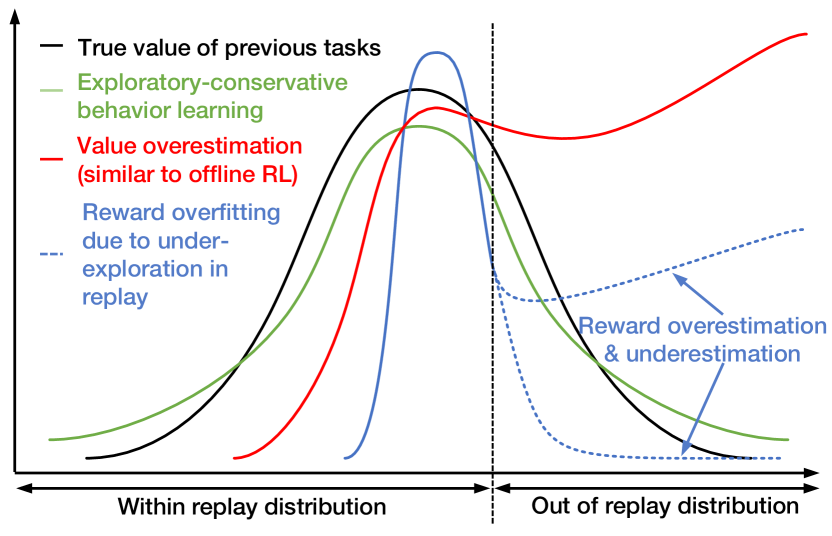
Figure 2: Intuition of the proposed exploratory-conservative behavior learning method, which is to address the value overestimation or underestimation problems caused by the limited diversity of replayed trajectories. It broadens the output distribution in predictive experience replay, while penalizing overestimated state values with a frozen value network learned in the previous task.

3 Approach

In this section, we present the details of our approach. The entire framework is named continual predictive learning with a short acronym of CPL, which mainly consists of three parts:

• Mixture world model: A new probabilistic future prediction network with a mixture of learnable Gaussian priors. It captures multimodal visual dynamics with explicit label inputs.

• Predictive experience replay: A new rehearsal-based training scheme. It trains the world model by generating trajectories of previous tasks to avoid forgetting problems caused by data distribution drift. It is more efficient in memory usage than the existing rehearsal-based continual RL approaches.

• Exploratory-conservative behavior learning: An improved MBRL approach for continual visual control. It handles the reward overestimation or underestimation problems of the RL agent caused by the limited diversity of replayed trajectories.

In Section 3.1, we first discuss the overall pipeline of CPL and its basic motivations. In Section 3.2 to Section 3.4, we respectively introduce the technical details of the three components.

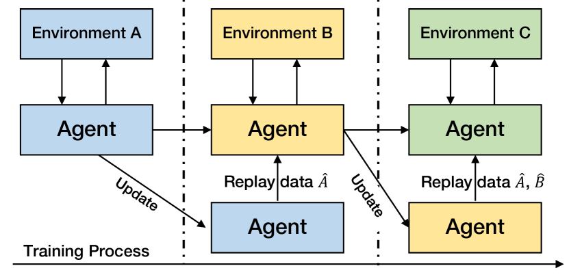
Figure 3: The overall pipeline of learning the mixture world model with predictive experience replay.

3.1 Overall Pipeline

We first briefly revisit the baseline model Dreamer [5] and introduce the overall pipeline of our CPL framework.

Revisiting Dreamer. Dreamer is an MBRL approach that tries to solve visual control tasks on latent imagination. The learning process of Dreamer can be summarized into two iterative stages: (i) world model learning of latent state transitions and reward predictions, and (ii) behavior learning via latent imagination. The world model $\mathcal{M}$ mainly contains four components:

$$\begin{split}\text{Representation module:}&\quad z_{t}\sim q_{\phi}({o}_{t},z_{t-1},a_{t-1})\\ \text{Transition module:}&\quad\hat{z}_{t}\sim p_{\psi}(z_{t-1},a_{t-1})\\ \text{Observation module:}&\quad\hat{o}_{t}=p_{{\theta}_{1}}(z_{t})\\ \text{Reward module:}&\quad\hat{r}_{t}=p_{{\theta}_{2}}(z_{t}).\\ \end{split}$$ (4)

In this stage, trajectory batches are sampled from the dataset of past experience and used to train the world model to predict future rewards and frames from actions and past observations. Then, in the behavior learning stage, Dreamer uses the learned world model to predict latent trajectories to train action and value models:

$$\begin{split}\text{Action model:}&\quad{a}_{t}\sim\pi(z_{t})\\ \text{Value model:}&\quad v(z_{t^{\prime}})\approx\mathbb{E}_{\pi\left(\cdot\mid z_{t^{\prime}},\right)}\sum_{t^{\prime}=t}^{t+L}\gamma^{t^{\prime}-t}r_{t^{\prime}},\end{split}$$ (5)

where $t^{\prime}$ is the time index of the imagined states, $L$ is the imagination time horizon, and $\gamma$ is the reward discount. The value model aims to optimize Bellman consistency for imagined rewards, and the action module is updated by back-propagating the gradients from the value estimation through the learned dynamics. Particularly, behavior learning is purely conducted on the latent trajectories without involving the observation module for image generation, which significantly accelerates the learning process.

Overall continual learning scheme of CPL. To adapt Dreamer to the continual RL setup, we make improvements in three aspects: the world model architecture, the world model learning scheme, and behavior learning. The overall learning pipeline is shown in Fig. 3, where the X-axis represents the training phases of sequential tasks. We first initialize the agent, including the world model $\mathcal{M}$, the actor $\pi$, and the critic $v$, and an initial-frame generator $\mathcal{G}$. Since the agent is not allowed to access real data of previous tasks, we will retain a copy of the current models after finishing the training process of a particular task, termed as $\mathcal{M}^{\prime}$, ${\pi}^{\prime}$, ${v}^{\prime}$, and $\mathcal{G^{\prime}}$. These models will be frozen and used to perform the imagination with image outputs to generate trajectories of previous tasks for replay. In other words, we train the models on sequential tasks but continually update one copy of them to involve increasingly more previous knowledge for rehearsal. This pipeline is at the heart of our approach. For the downstream control tasks, ideally reproducing prior knowledge as latent imagination is a cornerstone for alleviating the forgetting issues in behavior learning. Besides, the requirement of ideally reproducing prior knowledge also guides the detailed world model design.

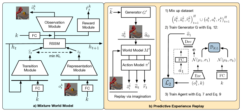
Figure 4: The details of the mixture world model and the predictive experience replay training scheme in the proposed CPL approach. (a) The world model learns representations in the forms of mixture-of-Gaussians based on categorical task variables. It uses a Recurrent State-Space Model (RSSM) [30] to provide deterministic hidden state $h$. (b) In predictive experience replay, we use an additional generative model for initial-frame generation (${\mathcal{G}}$). The models used for the replay are the copy of previously learned world model ${\mathcal{M}}^{\prime}$, action model ${\pi}^{\prime}$, and generative model ${\mathcal{G}}^{\prime}$. We first use ${\mathcal{G}}^{\prime}$ to generate the first frames of previous tasks, then use ${\mathcal{M}}^{\prime}$ and ${\pi}^{\prime}$ to iteratively predict future frames and rewards, and finally combine the rehearsal data and real data to jointly train the agent and the generative model.

3.2 Mixture World Model

The proposed mixture world model may have different encoding and decoding architectures when it is used in specific tasks, but they all follow a unified learning paradigm based on Gaussian mixture representations. Without loss of generality, we here take the network architecture in MBRL as an example to describe its representation learning method. Specifically, we improve the world model ${\mathcal{M}}$ in Dreamer [5] from the perspective of multimodal spatiotemporal modeling, which serves as the cornerstone to overcome catastrophic forgetting in continual visual control. For video prediction tasks, which are focused more on the generation quality in pixel space, we can simply replace the encoder and decoder with a more complex backbone. We provide the specific designs of the world model in sequential visual forecasting tasks in supplementary materials.

As discussed in Section 1, the co-existence of the covariate-dynamics-target shift in non-stationary environments causes the forgetting issue within existing world models. Therefore, the key challenge for the world model lies in how to be aware of the distribution shift and properly distinguish them. To address this challenge, as shown in Fig. 4(a), we exploit mixture-of-Gaussian variables to capture the multimodal distribution of both visual dynamics in the latent space and spatial appearance in the input/output observation space. Accordingly, the world model can be written as:

$$\begin{split}\text{Representation module:}&\quad z_{t}\sim q_{\phi}({o}_{t}^{k},z_{t-1},a_{t-1}^{k},k)\\ \text{Transition module:}&\quad\hat{z}_{t}\sim p_{\psi}(z_{t-1},a_{t-1}^{k},k)\\ \text{Observation module:}&\quad\hat{o}_{t}=p_{{\theta}_{1}}(z_{t},k)\\ \text{Reward module:}&\quad\hat{r}_{t}=p_{{\theta}_{2}}(z_{t},k).\\ \end{split}$$ (6)

The representation module aims to encode observations and actions to infer the latent state $z_{t}$. It also takes the categorical task variable $k\in\{1,\ldots,K\}$ as an extra input to handle the covariate shift in input space. The transition module is also aware of the categorical task variable and tries to predict latent state $\hat{z}_{t}$ to approximate the posterior state $z_{t}$. These modules are jointly optimized with the Kullback-Leibler divergence to learn the posterior and the prior distribution of the latent state $z_{t}$. Finally, the observation and reward modules take the state $z_{t}$ along with the task variable $k$ to reconstruct images and predict corresponding rewards.

In this model, the task-specific latent variables $z_{t}$ and $\hat{z}_{t}$ have the form of Gaussian mixture distributions conditioned on $k$, which shares a similar motivation with the Gaussian mixture priors proposed in existing unsupervised learning methods [31, 32, 33]. Compared with these methods, the mixture world model is an early work to explore the multimodal priors for modeling spatiotemporal dynamics. For task $\mathcal{T}_{k}$, the objective function of the world model combines the reconstruction loss of the input frames, the prediction loss of the rewards, and the KL divergence:

$$\begin{split}{\mathcal{L}}_{{\mathcal{M}}}&=\mathbb{E}\big{[}\sum\limits_{t=1}^{H}-\log p(\hat{o}_{t}\,|\,z_{t},k)-\log p(\hat{r}_{t}\,|\,z_{t},k)\\ &-\alpha D_{KL}(q(z_{t}\,|\,{o}_{t}^{k},z_{t-1},a_{t-1}^{k},k)\,||\,p(\hat{z}_{t}\,|\,z_{t-1},a_{t-1}^{k},k)\big{]},\end{split}$$ (7)

where $\alpha$ equals to $1.0$, and $({o}_{t}^{k},a_{t}^{k},r_{t}^{k})_{t=1}^{H}$ represents a training trajectory sampled from the data buffer in the current task or sampled from the model in predictive experience replay.

3.3 Predictive Experience Replay

In continual learning setups, the dilemma between continual performance and memory consumption is always the inevitable challenge for previous approaches. One popular solution to this challenge is generative replay [34], which exploits an extra generative model to reproduce samples of previous tasks. However, using a single generative model to reproduce high-quality trajectories is extremely difficult, which suggests that the original generative replay method can not be directly used in our setup.

Therefore, we introduce the predictive experience replay scheme, which firmly combines an initial-frame generative model with the agent to efficiently generate the trajectories of previous tasks. To overcome the covariant shift of the image appearance in time-varying environments, the introduced generative model also uses Gaussian mixture distributions to form the latent priors, denoted by $\boldsymbol{e}$. Specifically, as shown in Fig. 4(b), after training on the previous task, we first retain a copy of the generative model ${\mathcal{G}}$, the world model ${\mathcal{M}}$, and the action model $\pi$. These copies are respectively denoted as $\mathcal{G^{\prime}}$, $\mathcal{M^{\prime}}$, and ${\pi}^{\prime}$. Then, for each previous task $\mathcal{T}_{\tilde{k}<k}$, we use $\mathcal{G^{\prime}}$ to generate the initial frames of the rehearsal trajectories. Along with a zero-initialized action $a_{0}$, we iteratively perform $\mathcal{M^{\prime}}$ and $\mathcal{\pi}^{\prime}$ to generate future sequences:

$$\begin{split}\hat{o}^{\tilde{k}}_{0}&\leftarrow\mathcal{G^{\prime}}({\tilde{k}}),\\ \hat{o}_{t}^{\tilde{k}},\hat{z}_{t},\hat{r}_{t}^{\tilde{k}}&\leftarrow\mathcal{M^{\prime}}(\hat{o}^{\tilde{k}}_{t-1},\hat{a}_{t-1}^{\tilde{k}},{\tilde{k}}),\\ \hat{a}_{t}^{\tilde{k}}&\leftarrow\mathcal{\pi}^{\prime}(\hat{z}_{t},{\tilde{k}}).\end{split}$$ (8)

Finally, the replay trajectories $(\hat{o}_{t}^{\tilde{k}},\hat{a}_{t}^{\tilde{k}},\hat{r}_{t}^{\tilde{k}})_{t=1}^{H}$ and the real trajectories at the current task $\mathcal{T}_{k}$ are mixed together to train the generator and the agent in turn, and $\mathcal{G^{\prime}}$, $\mathcal{M^{\prime}}$, and $\mathcal{\pi}^{\prime}$ will be frozen and continually updated until the task stream ends. Since the world model is also involved in the replay process and plays a key role, the proposed predictive experience replay is significantly different from all previous generative replay methods.

During predictive experience replay at task $\mathcal{T}_{k}$, the world model ${\mathcal{M}}$ is trained by minimizing

$$\begin{split}{\mathcal{L}}_{{\mathcal{M}}}=\sum\limits_{\tilde{k}=1}^{k-1}{\mathcal{L}}_{{\mathcal{M}}}^{\tilde{k}}(\hat{o}_{1:H}^{\tilde{k}},\hat{a}_{1:H}^{\tilde{k}},\hat{r}_{1:H}^{\tilde{k}})+{\mathcal{L}}_{{\mathcal{M}}}^{k}(o_{1:H}^{k},a_{1:H}^{k},r_{1:H}).\\ \end{split}$$ (9)

The objective function of the initial-frame generator ${\mathcal{G}}$ can be written as

$$\begin{split}{\mathcal{L}}_{{\mathcal{G}}}&=\ \mathbb{E}_{q(\boldsymbol{e}\,|\,{{o}_{1}^{k},k})}\log p({o}_{1}^{k}\,|\,\boldsymbol{e},k)\\ &\quad-\beta D_{KL}(q(\boldsymbol{e}\,|\,{o}_{1}^{k},k)\,||\,p(\hat{\boldsymbol{e}}\,|\,k))\\ &+\sum\limits_{\tilde{k}=1}^{k-1}\big{[}\mathbb{E}_{q(\boldsymbol{e}\,|\,{\hat{{o}}_{1}^{\tilde{k}},{\tilde{k}}})}\log p(\hat{{o}}_{1}^{\tilde{k}}\,|\,\boldsymbol{e},{\tilde{k}})\\ &\quad-\beta D_{KL}(q(\boldsymbol{e}\,|\,\hat{{o}}_{1}^{\tilde{k}},{\tilde{k}})\,||\,p(\hat{\boldsymbol{e}}\,|\,{\tilde{k}}))\big{]},\\ \end{split}$$ (10)

where we use the $\ell_{2}$ loss for reconstruction and set $\beta$ equals to $10^{-4}$ through an empirical grid search.

3.4 Exploratory-Conservative Behavior Learning

If we simply combine the mixture world model with the predictive experience replay scheme, we will have a naïve solution to handle continual visual control tasks. However, as shown in Fig 5, on the Meta-World benchmark, we can observe that this naïve solution (indicated by the blue bars) can not mitigate the forgetting issue and may even degenerate the control performance on some tasks compared with Dreamer, such as the task Window-open.

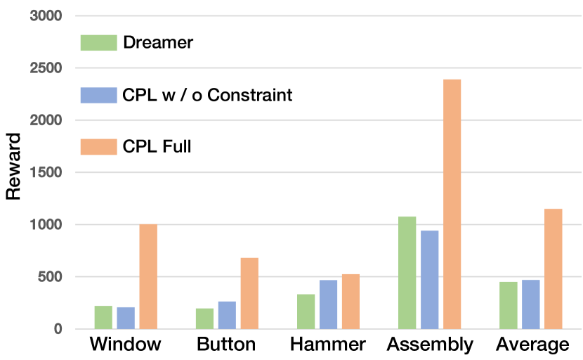
Figure 5: Effect of the proposed behavior learning method. We evaluate the model obtained after the last training task (i.e., Assembly on Meta-World) on each of the tasks represented on the X-axis. The task order is Window-open $\rightarrow$ Button-press $\rightarrow$ Hammer $\rightarrow$ Assembly. “CPL w/o Constraint” represents a baseline model without exploratory-conservative behavior learning.

We find that the performance degeneration is rooted in two closely related overfitting problems that happen respectively in world model learning and behavior learning. Both of them leads to the erroneous estimation of the value functions for previous tasks. As shown in Fig. 6, we use the same trajectory batches from the very first task (i.e., Window-open) to evaluate the outputs of the reward predictor and those of the value network after training these models on each subsequent task (i.e., Button-press $\rightarrow$ Hammer $\rightarrow$ Assembly). We observe that the world model produces inaccurate reward predictions, which can be caused by the narrow distribution of the replayed data. More significantly, we also observe overestimated values. This phenomenon is similar to previous findings in offline RL [25, 26].

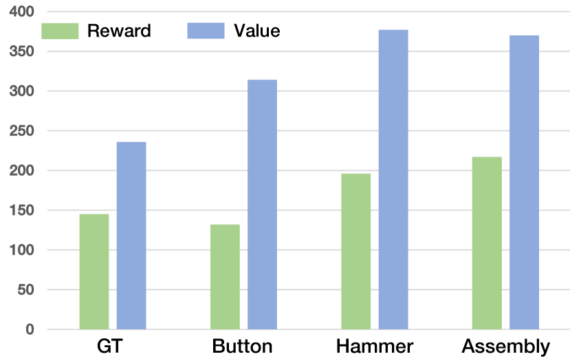
Figure 6: Reward predictions and value estimations in the naïve solution. We use $100$ batches of trajectories of Window-open to evaluate models trained after each subsequent task. We use the model trained on Window-open to calculate the “ground truth” of the state values. The X-axis represents different models that just finished training on corresponding tasks. The values are re-scaled for better visualization.

To tackle these problems, we propose the exploratory-conservative behavior learning method (see Alg. 1) that respectively improves the original predictive experience replay training scheme of the world model and the value estimation objectives for the rehearsal data in the actor-critic algorithm. The key idea is to broaden the output distribution in predictive experience replay and penalize overestimated state values with point-to-point constraints provided by a frozen value network that was learned in the previous task.

First, we introduce specific data argumentation for the reward predictor during predictive experience replay. The key insight lies in that we want the world model to experience more diverse observation-action pairs to keep it from overfitting the limited rehearsal data and thus underperforming for out-of-distribution samples. On one hand, we exploit the $\epsilon$-greedy strategy to improve action exploration to generate trajectories of previous tasks $(\hat{o}_{t}^{k},\hat{a}_{t}^{k},\hat{r}_{t}^{k})_{t=1}^{H}$. On the other hand, we randomly shuffle the generated actions and reuse the learned world model at the previous task ${\mathcal{M}}^{\prime}$ to predict new rewards, which results in a new trajectory $(\hat{o}_{t}^{k},\tilde{a}_{t}^{k},\tilde{r}_{t}^{k})_{t=1}^{H}$. Notably, these augmented trajectories are only used to train the reward predictor. They break the temporal biases in the distribution of rehearsal data and prevent the reward prediction from overfitting issues. We summarize this procedure in Alg. 2. Assuming $\tilde{z}_{t}$ represents the latent state extracted from the augmented data, the objective function of the world model in Eq. (7) can be rewritten as:

$$\begin{split}{\mathcal{L}}_{{\mathcal{M}}}&=\mathbb{E}\big{[}\sum\limits_{t=1}^{H}-\log p(\hat{o}_{t}\,|\,z_{t},k)-\log p(\hat{r}_{t}\,|\,z_{t},k)\\ &-\delta\log p(\tilde{r}_{t}\,|\,\texttt{sg}(\tilde{z}_{t}),k)-\alpha D_{KL}(q(z_{t}\,|\,{o}_{t}^{k},\cdot)\,||\,p(\hat{z}_{t}\,|\,\cdot)\big{]},\end{split}$$ (11)

where sg is the stop-gradient operation and $\delta$ equals to $0.5$ in all experiments.

Algorithm 1 Exploratory-conservative behavior learning

1:Task stream $\mathcal{T}_{1},,\ldots,\mathcal{T}_{K}$

2:World model ${\mathcal{M}}$, generator ${\mathcal{G}}$, and actor $\mathcal{\pi}$

3:Initial buffer $\mathcal{B}_{1}$ at $\mathcal{T}_{1}$ with random episodes

4:while not converged do

5:     Train ${\mathcal{G}}$ at $\mathcal{T}_{1}$ according to Eq. (10) with $k=1$

6:     Perform dynamics learning at $\mathcal{T}_{1}$ according to Eq. (7)

7:     Perform behavior learning at $\mathcal{T}_{1}$ according to Eq. (13)

8:     Add interaction experience to buffer $\mathcal{B}_{1}$

9:end while

10:for $k=2,\ldots,K$ do

11:     Initial buffer $\mathcal{B}_{k}$ at $\mathcal{T}_{k}$ with random episodes

12:     Retain a copy of previous model as $\mathcal{M^{\prime}}$, $\mathcal{G^{\prime}}$, $\mathcal{\pi^{\prime}}$ , and $v^{\prime}$

13:     # Predictive experience replay

14:     Generate replayed trajectory $\tau_{1}$ and augmented data $\tau_{2}$ with Alg. 2

15:     # Mix replayed data at $\mathcal{T}_{1:k-1}$ and real data at $\mathcal{T}_{k}$

16:     $\mathcal{B}_{k}^{\prime}\leftarrow\tau_{1}\cup\mathcal{B}_{k}$

17:     while not converged do

18:         Train ${\mathcal{G}}$ on $\mathcal{B}_{k}^{\prime}$ according to Eq. (10)

19:         Perform dynamics learning on $\mathcal{B}_{k}^{\prime}$ with Eq. (7)

20:         Perform behavior learning on $\mathcal{B}_{k}$ with Eq. (13)

21:         # Use reward augmentation

22:         Train reward module on $\tau_{2}$ with Eq. (11)

23:         # Use conservative value target

24:         Perform behavior learning on on $\tau_{1}$ with Eq. (14)

25:         Append interaction experience to $\mathcal{B}_{k}$

26:     end while

27:end for

Algorithm 2 Predictive experience replay with data augmentation

1:Current task label $k$, world model $\mathcal{M^{\prime}}$, generator $\mathcal{G^{\prime}}$, actor $\mathcal{{\pi}^{\prime}}$, and $\epsilon$ for action exploration in predictive experience replay

2:Replayed trajectories $\tau_{1}$ and $\tau_{2}$

3:Initial $\tau_{1}=\emptyset$, $\tau_{2}=\emptyset$

4:for $\tilde{k}=1,\ldots,k-1$ do

5:     # Replay trajectories (skip the batch size)

6:     $\hat{o}^{\tilde{k}}_{0}\leftarrow\mathcal{G^{\prime}}({\tilde{k}}),\hat{a}_{0}\leftarrow 0$

7:     for $t=1,\ldots,H$ do

8:         $\hat{o}_{t}^{\tilde{k}},\hat{z}_{t},\hat{r}_{t}^{\tilde{k}}\leftarrow\mathcal{M^{\prime}}(\hat{o}^{\tilde{k}}_{t-1},\hat{a}_{t-1}^{\tilde{k}},{\tilde{k}})$

9:         # Perform the $\epsilon$-greedy exploration.

10:         if $\eta\sim\mathcal{U}(0,1)<\epsilon$ then

11:              $\hat{a}_{t}^{\tilde{k}}\sim\mathcal{U}(-1,1)$

12:         else

13:              $\hat{a}_{t}^{\tilde{k}}\leftarrow\mathcal{\pi}^{\prime}(\hat{z}_{t},{\tilde{k}})$

14:         end if

15:     end for

16:     $\tau_{1}=\tau_{1}\cup(\hat{o}_{t}^{\tilde{k}},\hat{a}_{t}^{\tilde{k}},\hat{r}_{t}^{\tilde{k}})_{t=1}^{H}$

17:     # Data augmentation via action shuffling

18:     for $t=1,\ldots,H$ do

19:         Randomly sample actions from task $\tilde{k}$ in $\tau_{1}$ as $\tilde{a}_{t-1}^{\tilde{k}}$

20:         $\tilde{r}_{t}^{\tilde{k}}\leftarrow\mathcal{M^{\prime}}(\hat{o}^{\tilde{k}}_{t-1},\tilde{a}_{t-1}^{\tilde{k}},{\tilde{k}})$

21:     end for

22:     $\tau_{2}=\tau_{2}\cup(\hat{o}_{t}^{\tilde{k}},\tilde{a}_{t}^{\tilde{k}},\tilde{r}_{t}^{\tilde{k}})_{t=1}^{H}$

23:end for

Second, we constrain the target of the value model when performing behavior learning on the replayed data, which is inspired by conservative Q-learning (CQL) [25]. Given the world model that captures the latent dynamics, the behavior learning stage is performed on the task-specific latent imagination. We use $t^{\prime}$ to denote the time index of the imagined states. Starting at the posterior latent state $z_{t}$ inferred from the visual observation, we exploit the transition module, the reward predictor, and the action model to predict the following states and corresponding rewards in imagination, which are all guided by the explicit task label $k$. Then the action model and the value model will be optimized on the imagined trajectories:

$$\begin{split}\text{Action model:}&\quad{a}_{t}^{k}\sim\pi(z_{t},k)\\ \text{Value model:}&\quad v(z_{t^{\prime}},k)\approx\mathbb{E}_{\pi\left(\cdot\mid z_{t^{\prime}},k\right)}\sum_{t^{\prime}=t}^{t+L}\gamma^{t^{\prime}-t}r_{t^{\prime}},\end{split}$$ (12)

where $L$ is the imagination time horizon and $\gamma$ is the reward discount. The action model is optimized to maximize the value estimation, while the value model is optimized to approximate the expected imagined rewards. The training target for the value model on real data is:

$$V_{t}=r_{t}+{\lambda}_{t}\begin{cases}(1-\lambda)v(z_{t+1})+\lambda V_{t+1}&if\quad t<L,\\ v(z_{L})&if\quad t=L,\end{cases}$$ (13)

where $\lambda$ equals to $0.95$. We adopt the objective functions from DreamerV2 [35] to train these models. However, when learning on the replayed data, this objective may result in the overestimation problem as shown in Fig. 6. Therefore, we reuse the learned value model to update the target when training on replayed data. Given a replayed trajectory $(\hat{o}_{t}^{k},\hat{a}_{t}^{k},\hat{r}_{t}^{k})_{t=1}^{H}$, we first calculate the training target $V_{t}$ according to Eq. (13). We then retain a copy of the value model $v^{\prime}$ that was learned on the previous task, and use the same trajectory as above to produce another conservative target $\widetilde{V}_{t}$ with the same function. We use $\widetilde{V}_{t}$ to constrain the current value model to tackle the value overestimation problem for previous tasks. The final target for training the value model on the rehearsal data is

$$V_{t}^{\prime}=\begin{cases}V_{t}&if\quad V_{t}<\widetilde{V}_{t},\\ \widetilde{V}_{t}&if\quad V_{t}>=\widetilde{V}_{t}.\end{cases}$$ (14)

Alg. 1 gives the full training procedure of the exploratory-conservative behavior learning. With the above two improvements, it successfully extends MBRL algorithms to sequential visual control tasks.

4 Experiments

In this section, we validate the effectiveness of CPL on both continual visual control and continual video forecasting tasks.

4.1 Continual Visual Control

4.1.1 Implementation Details

Benchmarks. We exploit two RL platforms with rich visual observations to perform the quantitative and qualitative evaluation for continual visual control tasks:

• DeepMind Control Suite (DMC) [27]. It is a popular RL platform that contains various manually designed control tasks with an articulated-body simulation. We use the Walker as the base agent and construct a task stream including four different tasks, i.e., Walk $\rightarrow$ Uphill $\rightarrow$ Downhill $\rightarrow$ Nofoot. Nofoot represents the task in which we cannot control the right foot of the robot.

• Meta-World [28]. This platform contains 50 distinct robotic manipulation tasks with the same robot agent. We select four different tasks (i.e., Window-open $\rightarrow$ Button-press $\rightarrow$ Hammer $\rightarrow$ Assembly) to form a task stream for evaluation.

We provide some showcases in Fig. 7. We assume that the task label in the test phase is provided for all experiments. We use the same task order for comparisons between different methods, and without loss of generality, our approach is practical to different task orders (see Section 4.3).

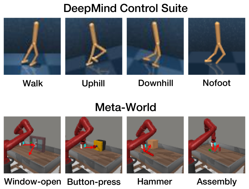
Figure 7: Showcases of the sequential visual control tasks.

Compared methods. We compare CPL with the following baselines and existing approaches:

• Dreamer [5]: It is an MBRL method and is also the baseline model that excludes the Gaussian mixture and the experience replay scheme from CPL. We compare CPL with this model in different setups including single-task training and full tasks continual training.

• CURL [36]: It is a model-free RL framework that exploits unsupervised representation learning to help high-level feature extraction from visual inputs. We use the version that uses SAC [37] for policy optimization.

• EWC [38]: It is a mainstream parameter-constrained continual learning method. We apply it to both Dreamer and CURL.

Training details. In all environments, the input image size is set to $64\times 64$, the batch size is $50$, and the imagination horizon is $50$. For each task in DMC, we train our method for $200$K iterations with action repeat equals to $1$, which results in $200$K environment steps. For each task in Meta-World, we train our method for $500$K iterations with action repeat equals to $2$, which results in $1$M environment steps. The probability in the $\epsilon$-greedy exploration is set to $0.2$ for all experiments. Notably, we find that the performance on the first task will significantly influence the qualities of replay data and the final performance. Therefore we adopt an early-stop strategy at the end of the first training task. The continual learning procedure will be allowed only if the agent achieves comparable performance compared with single-task training on the first task. Otherwise, we will restart the continual learning procedure. Besides, we save $200$ real images for each task to help the learning of the initial-frame generator $\mathcal{G}$. These images are only used to train the generator and do not contain any temporal relationships. More experimental configurations and the network details can be found in our GitHub repository.

Method	DeepMind Control Suite
	Walk	Uphill	Downhill	Nofoot	Average
Dreamer [2]	239 $\pm$ 156	181 $\pm$ 19	444 $\pm$178	936 $\pm$ 32	450
CURL [3]	539 $\pm$ 170	132 $\pm$ 64	133 $\pm$ 63	919 $\pm$ 46	431
Dreamer + EWC (hyper-1) [38]	744 $\pm$ 36	27 $\pm$ 12	70 $\pm$ 29	49 $\pm$ 40	223
Dreamer + EWC (hyper-2) [38]	705 $\pm$ 39	351 $\pm$ 133	292 $\pm$ 139	423 $\pm$ 182	443
CURL + EWC (hyper-3) [38]	206 $\pm$ 125	119 $\pm$ 90	186 $\pm$ 113	433 $\pm$ 322	236
CURL + EWC (hyper-4) [38]	222 $\pm$ 143	101 $\pm$ 59	409 $\pm$ 88	887 $\pm$ 75	405
CPL	606 $\pm$ 365	734 $\pm$ 346	954 $\pm$ 30	951 $\pm$ 19	812
Mixture World Model (Joint training)	951 $\pm$ 16	581 $\pm$ 120	903 $\pm$ 34	950 $\pm$ 16	846
Dreamer (Single training)	759 $\pm$ 24	343 $\pm$ 97	934$\pm$ 24	929 $\pm$ 35	741

TABLE I: Quantitative results of continual visual control on the DeepMind Control Suite. The task order is Walk $\rightarrow$ Uphill $\rightarrow$ Downhill $\rightarrow$ Nofoot, and we evaluate the model on all tasks after training on the last task Nofoot. (Lines 1-2) Existing RL methods with i.i.d. assumption. (Lines 3-6) Combinations of RL models and continual learning approaches, in which we try different hyper-parameters for the EWC method. (Lines 7) Our model that consists of the mixture world model, the predictive experience replay, and the exploratory-conservative behavior learning. (Line 8-9) Two baseline models including the model jointly trained on all tasks, whose results can be roughly viewed as the upper bound of our approach, and the model independently trained on a single task.

Method	Meta-World
	Window-open	Button-press	Hammer	Assembly	Average
Dreamer [2]	220 $\pm$ 33	195 $\pm$ 232	331 $\pm$196	1075 $\pm$ 37	451
CURL [3]	152 $\pm$ 37	51 $\pm$ 9	491 $\pm$ 38	862 $\pm$ 151	389
Dreamer + EWC [38]	549 $\pm$ 990	267 $\pm$ 105	448 $\pm$ 55	206 $\pm$ 10	367
CURL + EWC [38]	462 $\pm$ 450	265 $\pm$ 157	480 $\pm$ 41	202 $\pm$ 17	352
CPL	1004 $\pm$ 1251	681 $\pm$ 546	524 $\pm$ 333	2389 $\pm$ 676	1149
Mixture World Model (Joint training)	2119 $\pm$ 1528	2722 $\pm$ 516	2499 $\pm$ 895	2310 $\pm$ 418	2412
Dreamer (Single training)	3367 $\pm$ 954	2642 $\pm$ 840	950 $\pm$ 109	1283 $\pm$ 66	2060

TABLE II: Quantitative results of continual visual control on the Meta-World. The task order is Window-open $\rightarrow$ Button-press $\rightarrow$ Hammer $\rightarrow$ Assembly, and we evaluate the model on all tasks after training on the last task Assembly.

4.1.2 Quantitative Comparison

We run the continual learning procedure with $3$ seeds and report the mean rewards and standard deviations of $10$ episodes in Table I and Table II. We have the following observations for results on the DMC benchmark in Table I:

First, CPL achieves significant improvements compared with existing model-based and model-free RL approaches on all tasks. For example, CPL performs nearly $2.5\times$ high performance than Dreamer on the first learning task Walk, and the performance on the task Downhill is almost $7\times$ higher than CURL. These results show the CPL can effectively preserve the pre-learned knowledge throughout the continual learning procedure.

Second, CPL generally outperforms naïve combinations of EWC and popular RL approaches. CPL outperforms “CURL+EWC” on all tasks and performs better than “Dreamer+EWC” on three of four tasks. Notably, we find that the performance of EWC is sensitive to hyper-parameters when conducting continual visual control tasks. For each combination, we present the results using two different sets of hyper-parameters termed “hyper-1” to “hyper-4”. We can observe that the performance may change sharply when using different hyper-parameter sets. The reason may lie in that the extra concerns on the feature extraction module from visual inputs make EWC hard to well constrain pre-learned knowledge in parameters.

Third, CPL even outperforms the results of both joint training and single training on three of four tasks. If considering the average rewards on all tasks, CPL outperforms the single training results for a large margin ($811.5$ vs. $741.3$). It shows that our approach not only mitigates catastrophic forgetting issues but also improves the pre-learned tasks.

We can also find similar observations on the Meta-World benchmark in Table II. Our approach consistently outperforms previous RL methods and their naïve combinations with continual learning method EWC on all tasks. For instance, CPL achieves near $3\times$ average rewards compared with Dreamer and about $2.5\times$ average rewards compared with CURL. Notably, the result on the final task Assembly shows that CPL can effectively use the pre-learned knowledge to further improve the performance on the latter tasks. For the Assembly task, CPL outperforms the single training results for a large margin and even outperforms the joint training results. Combined with the results in the DMC benchmark, it seems that our framework has a huge potential in improving the forward transfer performance in continual visual control.

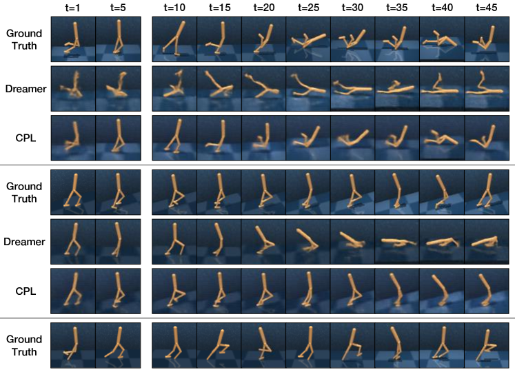
Figure 8: Visual forecasting results on the task Walk (upper) and Uphill (middle) after the model trained on the last task Nofoot (bottom). For each sequence, we use the first $5$ images as context frames and predict the next $45$ frames given actions. The world model in CPL effectively alleviates catastrophic forgetting, while Dreamer makes predictions similar to those in the last task.

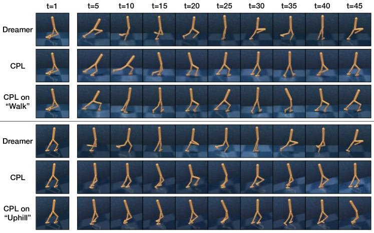
Figure 9: Imagination results on the task Walk (upper) and Uphill (bottom) after the model trained on the last task Nofoot. For each task, we use the same image as the initial frame and perform imagination to obtain the following $49$ frames. The third rows in the upper and the bottom parts respectively represent results from CPL trained on the “Walk” and the “Uphill” tasks.

4.1.3 Qualitative Comparison

We also conduct visual forecasting experiments on the DMC benchmark to explore whether the learned world model can preserve the pre-learned visual dynamics during the continual learning procedure. After training the models on the last task Nofoot, we randomly collect sequences of frames and actions during the test phases of the first two tasks Walk and Uphill. We input the first five frames to the learned world model and ask it to predict the next $45$ frames with actions input. The prediction results are shown in Fig. 8. From these prediction results, we can observe that although these models have been continually trained on different tasks, the world model in CPL still remembers the visual dynamics in previous tasks. It successfully forecasts future frames given the corresponding action inputs without forgetting. On the contrary, the results predicted by Dreamer suffer from severe blur effects and share a similar appearance with trajectories of the last task Nofoot. These results show that the world models in MBRL methods can not handle catastrophic forgetting.

Besides, we provide the imagination results in Fig. 9 to further evaluate the action model after the whole training period. We randomly collect images from the first two training tasks Walk and Uphill. For each task, we use one image as the initial frame and ask models to perform imaginations from this frame to generate the following $49$ frames. Apart from comparing with Dreamer, we also add results from the CPL trained on these two tasks for comparisons, which are termed as “CPL on Walk” and “CPL on Uphill”. These results do not suffer from catastrophic forgetting. From Fig. 9, we have two observations. First, Dreamer fails to generate correct imagination results according to the given initial frames. It can not distinguish different tasks and only produce results that are similar to the last task Nofoot. Second, CPL can generate reasonable imagination results given different input frames from different tasks, and the imagination shares high similarities with that when training on corresponding tasks These results show that CPL successfully overcomes the catastrophic forgetting issues within both world models and action models.

Method	Action-conditioned		Action-free
	PSNR↑	SSIM↑ ($\times 10^{-2}$)	PSNR↑	SSIM↑ ($\times 10^{-2}$)
SVG [2]	18.72 $\pm$ 0.61	68.59 $\pm$ 2.22	18.92 $\pm$0.51	68.08 $\pm$ 2.20
PredRNN [3]	19.45	66.38	19.56	69.92
PhyDNet [39]	19.60	68.68	21.00	75.47
PredRNN + LwF [40]	19.10	64.73	19.79	71.43
PredRNN + EWC [38]	21.15	74.72	21.15	78.02
CPL-base + EWC [38]	21.29 $\pm$ 0.30	75.16 $\pm$ 0.98	21.38 $\pm$ 0.18	76.68 $\pm$ 0.69
CPL-base	19.36 $\pm$ 0.00	63.57 $\pm$ 0.00	20.15 $\pm$ 0.02	71.15 $\pm$ 0.08
CPL-full	23.26 $\pm$ 0.10	80.72 $\pm$ 0.23	22.48 $\pm$ 0.03	78.84 $\pm$ 0.07
CPL-base (Joint training)	24.64 $\pm$ 0.01	83.73 $\pm$ 0.00	22.56 $\pm$ 0.01	79.57 $\pm$ 0.02

TABLE III: Quantitative results on the RoboNet benchmark in both action-conditioned and action-free setups. (Lines 1-3) Existing video prediction models with i.i.d. assumption. (Lines 4-6) Combinations of predictive models and continual learning approaches. (Lines 7-8) The mixture world model and its combinations with the predictive experience replay. (Line 9) A baseline model jointly trained on all tasks throughout the training procedure, whose results can be roughly viewed as the upper bound of our approach.

4.2 Continual Visual Forecasting

4.2.1 Implementation Details

Benchmarks. We construct two real-world benchmarks of sequential visual forecasting tasks:

• RoboNet [29]. The RoboNet dataset collects action-conditioned videos of robotic arms interacting with a variety of objects in various environments. We use the environments as guidance to divide the entire dataset into four tasks (i.e., Berkeley $\rightarrow$ Google $\rightarrow$ Penn $\rightarrow$ Stanford). For each task, we collect about $3{,}840$ training sequences and $960$ testing sequences.

• KTH action [41]. This dataset contains gray-scale videos which include $6$ types of human actions. We directly use the action labels to divide the dataset into $6$ tasks (i.e., Boxing $\rightarrow$ Clapping $\rightarrow$ Waving $\rightarrow$ Walking $\rightarrow$ Jogging $\rightarrow$ Running). For each task, we collect about $1{,}500$ training sequences and $800$ testing sequences on average. The results and related ablation studies on this benchmark are provided in the supplementary materials.

We randomly sample the task orders for the comparison. More experimental configurations and the network details can be found in our previous paper [23] and GitHub repository.

Evaluation criteria. We adopt SSIM and PSNR from previous literature [2, 3] to evaluate the prediction results. We run the continual learning procedure $10$ times and report the mean results and standard deviations in the two metrics.

Compared methods. We compare CPL with the following baselines and existing approaches, including some naïve combinations of popular continual learning methods and forecasting methods:

• CPL-base: A baseline model that excludes the new components of Gaussian mixtures and predictive replay.

• PredRNN [3], SVG [2], PhyDNet [39]: Popular visual forecasting models focused on stochastic, deterministic, and disentangled dynamics modeling respectively.

• LwF [40]: It is a distillation-based continual learning method built on the memory state of PredRNN [3].

• EWC [38]: It is a parameter-constrained continual learning method and we apply it to both PredRNN and CPL-base.

4.2.2 Results on the RoboNet Benchmark

We evaluate CPL on the real-world RoboNet benchmark, in which different continual learning tasks are divided by laboratory environments. Particularly, experiments on RoboNet contain two setups including action-conditioned and action-free visual forecasting. The former follows the common practice [42, 43] to train the world model to predict $10$ future frames from $2$ observations and corresponding action sequence at the $11$ time steps. We use the first $5$ frames in the action-free setup to predict the subsequent $10$ frames.

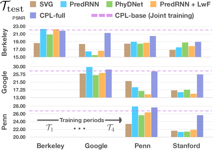
Figure 10: Results on the action-conditioned RoboNet benchmark. The horizontal axis represents the sequential training process, and the vertical axes represent test results on particular tasks after each training period. The purple dashed line indicates the results of the baseline model jointly trained on all tasks.

Quantitative comparison. Table III gives the quantitative results on RoboNet, in which we evaluate the models on the test sets of all $4$ tasks after the training period on the last task. We have the following observations here. First, CPL outperforms existing visual forecasting models by a large margin. For instance, in the action-conditioned setup, it outperforms SVG in PSNR by $24.3\%$, PredRNN by $19.6\%$, and PhyDNet by $18.7\%$. Second, CPL generally achieves better results than previous continual learning methods (i.e., LwF and EWC) combined with visual forecasting backbones. Note that a naïve implementation of LwF on top of PredRNN even leads to a negative effect on the final results. Third, by comparing CPL-full (our final approach) with CPL-base (w/o Gaussian mixture latents or predictive experience replay), we can see that the new technical contributions have a great impact on the performance gain. We provide more detailed ablation studies in Section 4.3. Finally, CPL is shown to effectively mitigate catastrophic forgetting by approaching the results of jointly training the world model on all tasks in the i.i.d. setting ($23.26$ vs. $24.64$ in PSNR). Apart from the average scores for all tasks, in Fig. 10, we provide the test results on particular tasks after individual training periods. As shown in the bar charts right to the main diagonal, CPL performs particularly well on previous tasks, effectively alleviating the forgetting issue.

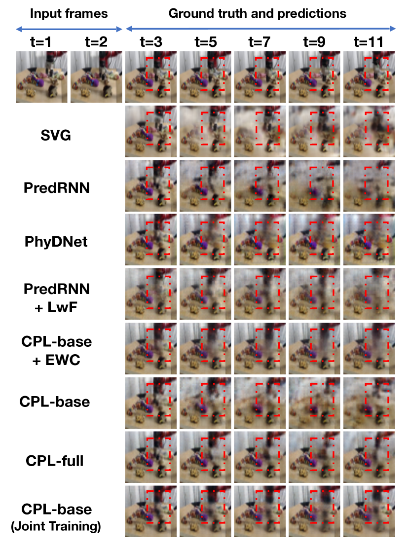
Figure 11: Showcases of action-conditioned visual forecasting in the first environment of RoboNet (i.e., Berkeley) after continually training the models in the last environment (i.e., Stanford).

Qualitative comparison. Fig. 11 shows the qualitative comparisons on the action-conditioned RoboNet benchmark. Specifically, we use the final models after the training period of the last task to make predictions on the first task. We can see from these results that our approach is more accurate in predicting both the future dynamics of the objects as well as the static information of the scene. In contrast, the predicted frames by PredRNN+LwF and CPL-base+EWC suffer from severe blur effect in the moving object or the static (but complex) background, indicating that directly combining existing continual learning algorithms with the world models cannot effectively cope with the dynamics shift in highly non-stationary environments.

4.3 Ablation Study

We conduct ablation studies on the DMC benchmark to evaluate different components in continual visual control. In Table IV, the first line provides the results of the baseline model which only contains the mixture world model, and the bottom line represents our final approach. In the second line, we train the baseline model with the pure predictive experience replay scheme, and we observe that the improvements are limited. As suggested in Section 3.4, the main reason lies in that training on the replay data only will result in overfitting problems on both the reward prediction and the value estimation. Then, as shown in the third line and the fourth line, we further improve the experience replay with the exploration-conservative behavior learning scheme. We gradually introduce the $\epsilon$-greedy exploration strategy and the data augmentation on the frame-action pairs and use them to regularize the learning of the reward module on replay trajectories. We can observe significant improvement compared with the pure replay scheme. Finally, in the bottom line, we reuse the pre-learned value model to introduce the constraint on the value estimation during the behavior learning stage. It also shows a large performance boost. We also experiment with different $\epsilon$ values in the $\epsilon$-greedy exploration and show the average rewards in Fig. 12. On one hand, slightly increasing the probability to introduce random actions can significantly improve the performance. On the other hand, excessively raising the $\epsilon$ value may introduce too many noises and degenerate the performance.

Besides, we additionally train the CPL model in $3$ random task orders on the DMC benchmark to analyze whether CPL can effectively alleviate catastrophic forgetting regardless of the task order. The mean reward with standard deviation is $801\pm 35$, which shows that the proposed techniques including the mixture world model and the predictive experience replay are still effective despite the change of training order. However, we find some tasks from the Meta-World benchmark suffer from huge standard deviations, which influence the robustness to different task orders. One reason may lie in that the environments in Meta-World contain more complex actions and more interactive objects, which makes it difficult to replay high-quality trajectories for rehearsal. We leave this challenge in our future work.

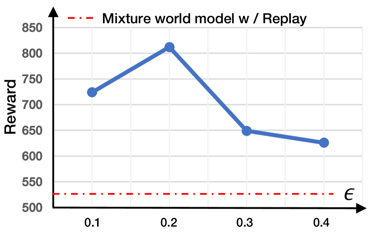
Figure 12: Ablation study of different $\epsilon$ values in the $\epsilon$-greedy exploration on the DMC visual control benchmark.

Replay	$\epsilon$-Greedy	$a$ Aug	$v$ Reg	Reward
✗	✗	✗	✗	450
✓	✗	✗	✗	525
✓	✓	✗	✗	616
✓	✓	✓	✗	788
✓	✓	✓	✓	812

TABLE IV: Ablation studies of each component in CPL on the DMC visual control benchmark. “Replay” denotes the use of predictive experience replay. “$\epsilon$-greedy” denotes the use of $\epsilon$-greedy exploration in collecting rehearsal data. “$a$ Aug” indicates using action augmentation in exploratory-conservative behavior learning. “$v$ Reg” means that the agent takes the previous value modal to constrain the value estimation.

5 Related Work

Continual learning. Continual learning is designed to cope with the continuous information flow, retaining or even optimizing old knowledge while absorbing new knowledge. Most existing approaches are mainly focused on supervised tasks of image data, and mainstream paradigms include regularization, replay, and parameter isolation [44]. The regularization approaches typically tackle catastrophic forgetting [45] by constraining the learned parameters on new tasks with additional loss terms, e.g., EWC [38], or distilling knowledge from old tasks, e.g., LwF [40]. For replay-based approaches, a typical solution is to retain a buffer on earlier tasks of representative data or feature exemplars [46, 47, 48]. Some approaches also use generative networks to encode the previous data distribution and synthesize fictitious data for experience replay, e.g., DGR [34]. The parameter isolation approaches allow the neural networks to dynamically expand when new tasks arrive [49] or encourage the new tasks to use previously “unused” parameter subspaces [50]. Despite the previous literature that discussed unsupervised continual learning [33, 51, 52], our approach is significantly different from these methods as it explores the specific challenges of continual learning of unsupervised video modeling, especially the covariate-dynamics-target shift.

Continual RL. Continual RL has become a hot topic in recent years [53, 54, 7, 9, 55]. To overcome catastrophic forgetting, a straightforward way is to explicitly retain pre-learned knowledge, which includes storage-based approaches that directly save task-dependent parameters [56] or priors [57, 58, 59], distillation based approaches [60, 61, 62] that leverages knowledge distillation [63] to recall previous knowledge, and the rehearsal based approaches that simply save trajectories [64, 65] or compact representations [66] for re-training. Besides, previous approaches [10, 8] mainly consider Markov Decision Process (MDP) with compact state space, which leaves the control tasks with high-dimensional visual inputs unexplored. Compared with these approaches, CPL focuses on the learning of the world model and proposes a new generative framework to tackle the forgetting issues in the context of the model-based RL approach. Instead of saving substantial trajectories, CPL only saves one copy of the model parameters and reuses the world model to perform predictive experience replay to retain previous knowledge, which results in a more effective and efficient approach. Besides knowledge retention, there are also approaches using shared structures to learn non-forgetting RL agents [67, 68].

RL for visual control. In visual control tasks, agents can only access high-dimensional observations. Previous approaches can be roughly summarized into two categories, that is, model-free approaches [69, 36, 70] and model-based approaches [30, 71, 72, 73]. Compared with MFRL approaches, the MBRL approaches explicitly learn the dynamic transitions and generally obtain higher sample efficiency. Ha and Schmidhuber proposed the World Model [4] with a two-stage training procedure that first learns latent transitions of the environment with self-supervision and then performs behavior learning on the states generated by the world model. PlaNet [30] introduces the RSSM network to optimize the policy over its recurrent states. The same architecture is also adopted by Dreamer [5] and DreamerV2 [35], where behavior learning is conducted on the latent imagination of RSSM. Recently, InfoPower [74] and Iso-Dream [6] further explore different ways to produce more robust dynamics representations for MBRL. In this paper, we make three improvements to adapt MBRL to continual visual control, i.e., the world model architecture, the world model learning scheme, and behavior learning.

Visual forecasting. RNN-based models have been widely used for deterministic visual forecasting [75, 76, 77, 78, 3]. Shi et al. [1] proposed ConvLSTM to improve the learning ability of spatial information by combining convolutions with LSTM transitions. Following this line, Wang et al. [75, 3] proposed PredRNN, modeling memory cells in a unified spatial and temporal representation. Stochastic visual forecasting models assume that different plausible outcomes would be equally probable for the same input, and thus incorporate uncertainty in the models using GANs [79] or VAEs [80, 81, 82]. Particularly, Yao et al. proposed to adapt visual forecasting models from multiple source domains to a target domain via distillation [78]. However, it cannot be easily used in our setup, as the number of retained model parameters increases linearly with the number of tasks.

Appendix A Specific Designs for Continual Visual Forecasting

A.1 World Model Architecture

For the continual visual forecasting problem, we propose some specific designs to improve the qualities of pixel-level predictions from two perspectives. On one hand, we remove the reward predictor in the world model and propose a new PredRNN-based [3] recurrent architecture which consists of three components:

$$\begin{split}\text{Representation module:}&\quad z_{t}\sim q_{\phi}({o}_{1:t}^{k},k)\\ \text{Encoding module:}&\quad\hat{z}_{t}\sim p_{\psi}({o}_{1:t-1}^{k},k)\\ \text{Transition module:}&\quad\widehat{o}_{t}=p_{\theta}(o_{1:t-1}^{k},a_{1:t-1}^{k},z_{1:t},k).\\ \end{split}$$ (15)

The representation module aims to infer the latent state $z_{t}$ from the ground truth frames. It takes the categorical task variable $k\in\{1,\ldots,K\}$ as extra input to cope with the target shift in input observation space. The encoding module instead maps the input frames to $\hat{z}_{t}$ to approximate the target state $z_{t}$, which focuses on the covariate shift in latent space. We also modify the transition module to improve the world model to capture the deterministic transition component from inputs and reconstruct target frames. It handles the multi-modal spatiotemporal dynamics by taking the task-specific latent variable $z_{t}$ and corresponding task variable $k$ as extra conditions. These modules are jointly optimized with the Kullback-Leibler divergence to learn the posterior and the prior distribution of the latent representation $z_{t}$. For task $\mathcal{T}_{k}$, the objective function of the world model combines the reconstruction loss and the KL loss:

$$\begin{split}\sum\limits_{t=2}^{T+H}&\big{[}\mathbb{E}_{q(z_{1:t}\,|\,{{o}_{1:t}^{k},k})}\log p({o}_{t}^{k}\,|\,{o}_{1:t-1}^{k},a_{1:t-1}^{k},z_{1:t},k)\\ &-\alpha D_{KL}(q(z_{t}\,|\,{o}_{1:t}^{k},k)\,||\,p(\hat{z}_{t}\,|\,{o}_{1:t-1}^{k},k))\big{]},\\ \end{split}$$ (16)

where $\alpha$ is set to $10^{-4}$ in our experiments. In the test phase, the representation module $q_{\phi}$ is dropped and the dynamics module uses sampled task-specific state $\hat{z}_{t}$ from the encoding module $p_{\psi}$ to predict future frames.

A.2 Non-Parametric Task Inference

On the other hand, we further propose a non-parametric task inference strategy to handle task ambiguity during the test phase. In the mixture world model, the task label plays a key role in not only learning distinguishing priors but also predicting high-quality results. Since it is unknown in the test phase of visual forecasting, a straightforward way is to directly use a video classification model to infer the label from test sequences. Nevertheless, using an extra classification model introduces more parameters and increases the risk of the catastrophic forgetting problem when jointly trained with the world model. To avoid using extra model-based task inference modules, we propose a new non-parametric inference strategy that reuses the learned world model to find the optimal task label.

Algorithm 3 Testing procedure

1:Observation frames $o_{1:T}$, optional actions $a_{1:T+H}$

2:Predicted future frames $\widehat{o}_{T+1:T+H}$

3:# Non-parametric task inference

4:for $k=1,\ldots,K$ do

5:     $\widehat{o}_{T/2+1:T}^{k}\leftarrow{\mathcal{M}}(o_{1:T/2},a_{1:T-1},k)$

6:end for

7:$\hat{k}=\arg\min_{k\in\{1,\ldots,K\}}\sum_{t=T/2+1}^{T}(o_{t}-\widehat{o}_{t}^{k})^{2}$

8:# Test-time adaptation (optional)

9:Optimize $\mathcal{M}$ with ${\mathcal{L}}_{{\mathcal{M}}}^{\hat{k}}({o}_{1:T},a_{1:T-1})$

10:# Model deployment

11:$\widehat{o}_{T+1:T+H}\leftarrow{\mathcal{M}}(o_{1:T},a_{1:T+H-1},\hat{k})$

More precisely, as shown in Alg. 3, we divide each test sequence $o_{1:T}$ to form a new sub-task that uses the first half sequence $o_{1:T/2}$ to predict the following half sequence. We then input $o_{1:T/2}$ along with the enumerated task label $k\in\{1,\ldots,K\}$ to the world model and evaluate its prediction results on the remaining test frames $o_{T/2+1:T}$. Finally, the task label $\hat{k}$ that can result in the best prediction quality will be selected as the final test label.

In addition to using $P(o_{T/2+1:T}|o_{1:T/2})$ for task inference, we also explore this self-supervision to perform test-time adaptation, which enables the model to continue learning after deployment. Through the one-step (or few-steps) online optimization on the inferred task ${\mathcal{T}}_{\hat{k}}$, test-time adaptation effectively recalls the pre-learned knowledge and further alleviates the forgetting issue.

Appendix B Visual Forecasting Results on KTH

Method	PSNR	SSIM ($\times 10^{-2}$)
SVG [2]	22.20 $\pm$ 0.02	69.23 $\pm$ 0.01
PredRNN [3]	23.27	70.47
PhyDNet [39]	23.68	72.97
PredRNN + LwF [40]	24.25	70.93
CPL-base + EWC [38]	24.32 $\pm$ 0.15	69.02 $\pm$ 0.48
CPL-base	22.96 $\pm$ 0.05	68.98 $\pm$ 0.02
CPL-full	29.12 $\pm$ 0.03	84.50 $\pm$ 0.04
CPL-base (Joint train)	28.12 $\pm$ 0.01	82.16 $\pm$ 0.00

TABLE V: Quantitative results on the KTH benchmark.

B.1 Quantitative Comparison

Table V provides the quantitative results on the test sets of all $6$ tasks after the last training period of the models on the last task. We can observe that CPL significantly outperforms the compared visual forecasting methods and continual learning methods in both PSNR and SSIM. Furthermore, an interesting result is that our approach even outperforms the joint training model, as shown in the bottom line in Table V. While we do not know the exact reasons, we state two hypotheses that can be investigated in future work. First, the Gaussian mixture priors enable the world model to better disentangle the representations of visual dynamics learned in different continual learning tasks. Second, the predictive experience replay allows the pre-learned knowledge on previous tasks to facilitate the learning process on new tasks. Fig. 13 shows the intermediate test results on particular tasks after each training period, which further confirms the above conclusions.

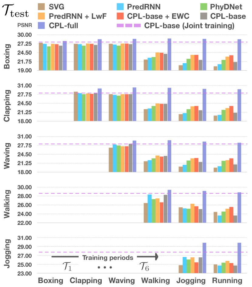
Figure 13: Results on the KTH benchmark. The horizontal axis represents the sequential training process, and the vertical axes represent test results on particular tasks after each training period.

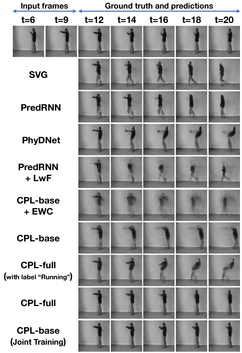
Figure 14: Showcases of predicted frames of the first task (i.e., Boxing) after the training period of the last task (i.e., Running).

B.2 Qualitative Comparison

In Fig. 14, we visualize a sequence of predicted frames on the first task of KTH after the entire continual training period. As shown, all existing visual forecasting models and even the one with LwF generate future frames with the dynamics learned in the last task (i.e., Running) instead of the first task (i.e., Boxing), which clearly demonstrates the influence of the dynamics shift. On the other hand, images generated by CPL-base+EWC suffer from severe blur effects, indicating that the model cannot learn disentangled representations for different dynamics in non-stationary training environments. In comparison, CPL produces more reasonable results. To testify the necessity of task inference, we also provide incorrect task labels for CPL. As shown in the third line from the bottom, the model takes as input the Boxing frames along with an erroneous task label of Running. Interestingly, CPL combines the inherent dynamics of input frames (reflected in the motion of arms) with the dynamics priors from the input task label (reflected in the motion of legs).

Appendix C Ablation Studies for Visual Forecasting

C.1 Effectiveness of Model Components

We conduct ablation studies on the sequential visual forecasting tasks step by step. In Table VI, the first line shows the results of the CPL-base model, and the bottom line corresponds to our final approach. In the second line, we train CPL-base with predictive experience replay only and observe a significant improvement from $22.96$ to $27.21$ in PSNR. In the third line, we improve the world model with mixture-of-Gaussian priors and accordingly perform non-parametric task inference at test time. We observe consistent improvements in both PSNR and SSIM upon the previous version of the model. In the fourth line, we skip the non-parametric task inference during testing and use a random task label instead. We observe that the performance drops from $27.82$ to $26.56$ in PSNR, indicating the importance of task inference to predictive experience replay. Finally, in the bottom line, we introduce the self-supervised test-time adaptation. It shows a remarkable performance boost compared with all the above variants.

Replay	Infer ${k}$	Random ${k}$	Adapt	PSNR	SSIM
✗	✗	✗	✗	22.96	68.98
✓	✗	✗	✗	27.21	79.99
✓	✓	✗	✗	27.82	81.51
✓	✗	✓	✗	26.56	78.64
✓	✓	✗	✓	29.12	84.50

TABLE VI: Ablation study for each component of CPL on the KTH benchmark. “Replay” denotes the use of predictive experience replay. “Infer $k$” indicates the use of non-parametric task inference. “Random $k$” means that the world model takes as input a random task label at test time. “Adapt” means test-time adaptation.

Dataset	PSNR	SSIM ($\times 10^{-2}$)
RoboNet	23.58 $\pm$ 0.28	79.67 $\pm$ 3.75
KTH	28.93 $\pm$ 0.14	83.99 $\pm$ 0.40

TABLE VII: Robustness of CPL on random task orders.

C.2 Robustness to Task Order

As shown in Table VII, we further conduct experiments to analyze whether CPL can effectively alleviate catastrophic forgetting regardless of the task order. We additionally train the CPL model in $3$-$4$ random task orders to obtain these results From the results, we find that the proposed techniques including the mixture world model, predictive experience replay, and non-parametric task inference are still effective despite the change in training order.

References

- [1] X. Shi, Z. Chen, H. Wang, D.-Y. Yeung, W.-K. Wong, and W.-c. Woo, “Convolutional LSTM network: A machine learning approach for precipitation nowcasting,” in NeurIPS, 2015, pp. 802–810.
- [2] E. Denton and R. Fergus, “Stochastic video generation with a learned prior,” in ICML, 2018, pp. 1182–1191.
- [3] Y. Wang, H. Wu, J. Zhang, Z. Gao, J. Wang, S. Y. Philip, and M. Long, “Predrnn: A recurrent neural network for spatiotemporal predictive learning,” IEEE Transactions on Pattern Analysis and Machine Intelligence, vol. 45, no. 2, pp. 2208–2225, 2022.
- [4] D. Ha and J. Schmidhuber, “Recurrent world models facilitate policy evolution,” in NeurIPS, vol. 31, 2018.
- [5] D. Hafner, T. Lillicrap, J. Ba, and M. Norouzi, “Dream to control: Learning behaviors by latent imagination,” in ICLR, 2020.
- [6] M. Pan, X. Zhu, Y. Wang, and X. Yang, “Iso-dream: Isolating and leveraging noncontrollable visual dynamics in world models,” in NeurIPS, 2022.
- [7] M. Wolczyk, M. Zajac, R. Pascanu, L. Kucinski, and P. Milos, “Continual world: A robotic benchmark for continual reinforcement learning,” in NeurIPS, 2021, pp. 28 496–28 510.
- [8] A. Xie and C. Finn, “Lifelong robotic reinforcement learning by retaining experiences,” in Conference on Lifelong Learning Agents, 2022, pp. 838–855.
- [9] S. Powers, E. Xing, E. Kolve, R. Mottaghi, and A. Gupta, “Cora: Benchmarks, baselines, and metrics as a platform for continual reinforcement learning agents,” in Conference on Lifelong Learning Agents, 2022, pp. 705–743.
- [10] W. Zhou, S. Bohez, J. Humplik, N. Heess, A. Abdolmaleki, D. Rao, M. Wulfmeier, and T. Haarnoja, “Forgetting and imbalance in robot lifelong learning with off-policy data,” in Conference on Lifelong Learning Agents, 2022, pp. 294–309.
- [11] H. Shimodaira, “Improving predictive inference under covariate shift by weighting the log-likelihood function,” Journal of statistical planning and inference, vol. 90, no. 2, pp. 227–244, 2000.
- [12] M. Sugiyama, S. Nakajima, H. Kashima, P. Von Buenau, and M. Kawanabe, “Direct importance estimation with model selection and its application to covariate shift adaptation.” in NeurIPS, vol. 7, 2007, pp. 1433–1440.
- [13] A. Gretton, A. Smola, J. Huang, M. Schmittfull, K. Borgwardt, and B. Schölkopf, “Covariate shift by kernel mean matching,” Dataset shift in machine learning, vol. 3, no. 4, p. 5, 2009.
- [14] M. Long, H. Zhu, J. Wang, and M. I. Jordan, “Deep transfer learning with joint adaptation networks,” in ICML, 2017, pp. 2208–2217.
- [15] M. Long, Y. Cao, J. Wang, and M. Jordan, “Learning transferable features with deep adaptation networks,” in ICML, 2015, pp. 97–105.
- [16] M. Long, Z. Cao, J. Wang, and M. I. Jordan, “Conditional adversarial domain adaptation,” in NeurIPS, 2017.
- [17] H. Liu, M. Long, J. Wang, and M. Jordan, “Transferable adversarial training: A general approach to adapting deep classifiers,” in ICML, 2019, pp. 4013–4022.
- [18] K. Zhang, B. Schölkopf, K. Muandet, and Z. Wang, “Domain adaptation under target and conditional shift,” in ICML, 2013, pp. 819–827.
- [19] A. Iyer, S. Nath, and S. Sarawagi, “Maximum mean discrepancy for class ratio estimation: Convergence bounds and kernel selection,” in ICML, 2014, pp. 530–538.
- [20] Z. Lipton, Y.-X. Wang, and A. Smola, “Detecting and correcting for label shift with black box predictors,” in ICML, 2018, pp. 3122–3130.
- [21] K. Azizzadenesheli, A. Liu, F. Yang, and A. Anandkumar, “Regularized learning for domain adaptation under label shifts,” arXiv preprint arXiv:1903.09734, 2019.
- [22] J. Guo, M. Gong, T. Liu, K. Zhang, and D. Tao, “LTF: A label transformation framework for correcting label shift,” in ICML, 2020, pp. 3843–3853.
- [23] G. Chen, W. Zhang, H. Lu, S. Gao, Y. Wang, M. Long, and X. Yang, “Continual predictive learning from videos,” in CVPR, 2022, pp. 10 728–10 737.
- [24] S. Fujimoto, D. Meger, and D. Precup, “Off-policy deep reinforcement learning without exploration,” in ICML, vol. 97, 2019, pp. 2052–2062.
- [25] A. Kumar, A. Zhou, G. Tucker, and S. Levine, “Conservative q-learning for offline reinforcement learning,” in NeurIPS, 2020.
- [26] Z. Wang, A. Novikov, K. Zolna, J. Merel, J. T. Springenberg, S. E. Reed, B. Shahriari, N. Y. Siegel, Ç. Gülçehre, N. Heess, and N. de Freitas, “Critic regularized regression,” in NeurIPS, 2020.
- [27] Y. Tassa, Y. Doron, A. Muldal, T. Erez, Y. Li, D. d. L. Casas, D. Budden, A. Abdolmaleki, J. Merel, A. Lefrancq et al., “Deepmind control suite,” arXiv preprint arXiv:1801.00690, 2018.
- [28] T. Yu, D. Quillen, Z. He, R. Julian, K. Hausman, C. Finn, and S. Levine, “Meta-world: A benchmark and evaluation for multi-task and meta reinforcement learning,” in CoRL, vol. 100, 2019, pp. 1094–1100.
- [29] S. Dasari, F. Ebert, S. Tian, S. Nair, B. Bucher, K. Schmeckpeper, S. Singh, S. Levine, and C. Finn, “Robonet: Large-scale multi-robot learning,” in CoRL, 2019, pp. 885–897.
- [30] D. Hafner, T. Lillicrap, I. Fischer, R. Villegas, D. Ha, H. Lee, and J. Davidson, “Learning latent dynamics for planning from pixels,” in ICML, 2019, pp. 2555–2565.
- [31] N. Dilokthanakul, P. A. Mediano, M. Garnelo, M. C. Lee, H. Salimbeni, K. Arulkumaran, and M. Shanahan, “Deep unsupervised clustering with gaussian mixture variational autoencoders,” arXiv preprint arXiv:1611.02648, 2016.
- [32] Z. Jiang, Y. Zheng, H. Tan, B. Tang, and H. Zhou, “Variational deep embedding: An unsupervised and generative approach to clustering,” in IJCAI, 2017, pp. 1965––1972.
- [33] D. Rao, F. Visin, A. A. Rusu, Y. W. Teh, R. Pascanu, and R. Hadsell, “Continual unsupervised representation learning,” in NeurIPS, 2019.
- [34] H. Shin, J. K. Lee, J. Kim, and J. Kim, “Continual learning with deep generative replay,” in NeurIPS, 2017, pp. 2990–2999.
- [35] D. Hafner, T. P. Lillicrap, M. Norouzi, and J. Ba, “Mastering atari with discrete world models,” in ICLR, 2021.
- [36] M. Laskin, A. Srinivas, and P. Abbeel, “CURL: contrastive unsupervised representations for reinforcement learning,” in ICML, 2020, pp. 5639–5650.
- [37] T. Haarnoja, A. Zhou, P. Abbeel, and S. Levine, “Soft actor-critic: Off-policy maximum entropy deep reinforcement learning with a stochastic actor,” in ICML, vol. 80, 2018, pp. 1856–1865.
- [38] J. Kirkpatrick, R. Pascanu, N. Rabinowitz, J. Veness, G. Desjardins, A. A. Rusu, K. Milan, J. Quan, T. Ramalho, A. Grabska-Barwinska et al., “Overcoming catastrophic forgetting in neural networks,” Proceedings of the national academy of sciences, vol. 114, no. 13, pp. 3521–3526, 2017.
- [39] V. L. Guen and N. Thome, “Disentangling physical dynamics from unknown factors for unsupervised video prediction,” in CVPR, 2020, pp. 11 474–11 484.
- [40] Z. Li and D. Hoiem, “Learning without forgetting,” IEEE transactions on pattern analysis and machine intelligence, vol. 40, no. 12, pp. 2935–2947, 2017.
- [41] C. Schüldt, I. Laptev, and B. Caputo, “Recognizing human actions: A local SVM approach,” in ICPR, 2004, pp. 32–36.
- [42] M. Babaeizadeh, C. Finn, D. Erhan, R. H. Campbell, and S. Levine, “Stochastic variational video prediction,” in ICLR, 2018.
- [43] B. Wu, S. Nair, R. Martín-Martín, L. Fei-Fei, and C. Finn, “Greedy hierarchical variational autoencoders for large-scale video prediction,” in CVPR, 2021, pp. 2318–2328.
- [44] M. Delange, R. Aljundi, M. Masana, S. Parisot, X. Jia, A. Leonardis, G. Slabaugh, and T. Tuytelaars, “A continual learning survey: Defying forgetting in classification tasks,” IEEE Transactions on Pattern Analysis and Machine Intelligence, 2021.
- [45] I. J. Goodfellow, M. Mirza, D. Xiao, A. Courville, and Y. Bengio, “An empirical investigation of catastrophic forgetting in gradient-based neural networks,” arXiv preprint arXiv:1312.6211, 2013.
- [46] S.-A. Rebuffi, A. Kolesnikov, G. Sperl, and C. H. Lampert, “iCaRL: Incremental classifier and representation learning,” in CVPR, 2017, pp. 2001–2010.
- [47] M. Riemer, I. Cases, R. Ajemian, M. Liu, I. Rish, Y. Tu, and G. Tesauro, “Learning to learn without forgetting by maximizing transfer and minimizing interference,” in ICLR, 2019.
- [48] A. Ayub and A. R. Wagner, “EEC: Learning to encode and regenerate images for continual learning,” in ICLR, 2021.
- [49] A. A. Rusu, N. C. Rabinowitz, G. Desjardins, H. Soyer, J. Kirkpatrick, K. Kavukcuoglu, R. Pascanu, and R. Hadsell, “Progressive neural networks,” arXiv preprint arXiv:1606.04671, 2016.
- [50] X. He and H. Jaeger, “Overcoming catastrophic interference using conceptor-aided backpropagation,” in ICLR, 2018.
- [51] H. Cha, J. Lee, and J. Shin, “Co2l: Contrastive continual learning,” in ICCV, 2021, pp. 9516–9525.
- [52] Z. Ke, B. Liu, H. Xu, and L. Shu, “Classic: Continual and contrastive learning of aspect sentiment classification tasks,” in EMNLP, 2021, pp. 6871–6883.
- [53] K. Khetarpal, M. Riemer, I. Rish, and D. Precup, “Towards continual reinforcement learning: A review and perspectives,” Journal of Artificial Intelligence Research, vol. 75, pp. 1401–1476, 2022.
- [54] R. Hadsell, D. Rao, A. A. Rusu, and R. Pascanu, “Embracing change: Continual learning in deep neural networks,” Trends in cognitive sciences, vol. 24, no. 12, pp. 1028–1040, 2020.
- [55] A. Xie, J. Harrison, and C. Finn, “Deep reinforcement learning amidst lifelong non-stationarity,” arXiv preprint arXiv:2006.10701, 2020.
- [56] H. B. Ammar, E. Eaton, P. Ruvolo, and M. Taylor, “Online multi-task learning for policy gradient methods,” in ICML, 2014, pp. 1206–1214.
- [57] G. Shi, K. Azizzadenesheli, M. O’Connell, S.-J. Chung, and Y. Yue, “Meta-adaptive nonlinear control: Theory and algorithms,” in NeurIPS, 2021, pp. 10 013–10 025.
- [58] T. Yu, S. Kumar, A. Gupta, S. Levine, K. Hausman, and C. Finn, “Gradient surgery for multi-task learning,” in NeurIPS, 2020, pp. 5824–5836.
- [59] B. Liu, X. Liu, X. Jin, P. Stone, and Q. Liu, “Conflict-averse gradient descent for multi-task learning,” in NeurIPS, 2021, pp. 18 878–18 890.
- [60] T. Zhang, X. Wang, B. Liang, and B. Yuan, “Catastrophic interference in reinforcement learning: A solution based on context division and knowledge distillation,” IEEE Transactions on Neural Networks and Learning Systems, 2022.
- [61] Q. Lan, Y. Pan, J. Luo, and A. R. Mahmood, “Memory-efficient reinforcement learning with knowledge consolidation,” arXiv preprint arXiv:2205.10868, 2022.
- [62] M. Igl, G. Farquhar, J. Luketina, J. Böhmer, and S. Whiteson, “Transient non-stationarity and generalisation in deep reinforcement learning,” in ICLR, 2021.
- [63] G. Hinton, O. Vinyals, and J. Dean, “Distilling the knowledge in a neural network,” arXiv preprint arXiv:1503.02531, 2015.
- [64] Z. A. Daniels, A. Raghavan, J. Hostetler, A. Rahman, I. Sur, M. Piacentino, A. Divakaran, R. Corizzo, K. Faber, N. Japkowicz et al., “Model-free generative replay for lifelong reinforcement learning: Application to starcraft-2,” in Conference on Lifelong Learning Agents, 2022, pp. 1120–1145.
- [65] P. Liotet, F. Vidaich, A. M. Metelli, and M. Restelli, “Lifelong hyper-policy optimization with multiple importance sampling regularization,” in AAAI, vol. 36, no. 7, 2022, pp. 7525–7533.
- [66] M. Riemer, T. Klinger, D. Bouneffouf, and M. Franceschini, “Scalable recollections for continual lifelong learning,” in AAAI, vol. 33, no. 01, 2019, pp. 1352–1359.
- [67] J. A. Mendez, H. van Seijen, and E. Eaton, “Modular lifelong reinforcement learning via neural composition,” arXiv preprint arXiv:2207.00429, 2022.
- [68] J. A. Mendez and E. Eaton, “How to reuse and compose knowledge for a lifetime of tasks: A survey on continual learning and functional composition,” arXiv preprint arXiv:2207.07730, 2022.
- [69] D. Yarats, A. Zhang, I. Kostrikov, B. Amos, J. Pineau, and R. Fergus, “Improving sample efficiency in model-free reinforcement learning from images,” in AAAI, vol. 35, no. 12, 2021, pp. 10 674–10 681.
- [70] I. Kostrikov, D. Yarats, and R. Fergus, “Image augmentation is all you need: Regularizing deep reinforcement learning from pixels,” arXiv preprint arXiv:2004.13649, 2020.
- [71] N. Hansen, Y. Lin, H. Su, X. Wang, V. Kumar, and A. Rajeswaran, “Modem: Accelerating visual model-based reinforcement learning with demonstrations,” arXiv preprint arXiv:2212.05698, 2022.
- [72] R. Sekar, O. Rybkin, K. Daniilidis, P. Abbeel, D. Hafner, and D. Pathak, “Planning to explore via self-supervised world models,” in ICML, 2020, pp. 8583–8592.
- [73] A. Zhang, R. McAllister, R. Calandra, Y. Gal, and S. Levine, “Learning invariant representations for reinforcement learning without reconstruction,” arXiv preprint arXiv:2006.10742, 2020.
- [74] H. Bharadhwaj, M. Babaeizadeh, D. Erhan, and S. Levine, “Information prioritization through empowerment in visual model-based RL,” in ICLR, 2022.
- [75] Y. Wang, M. Long, J. Wang, Z. Gao, and S. Y. Philip, “PredRNN: Recurrent neural networks for predictive learning using spatiotemporal lstms,” in NeurIPS, 2017, pp. 879–888.
- [76] Y. Wang, L. Jiang, M.-H. Yang, L.-J. Li, M. Long, and L. Fei-Fei, “Eidetic 3D LSTM: A model for video prediction and beyond,” in ICLR, 2019.
- [77] J. Su, W. Byeon, F. Huang, J. Kautz, and A. Anandkumar, “Convolutional tensor-train lstm for spatio-temporal learning,” in NeurIPS, 2020.
- [78] Z. Yao, Y. Wang, M. Long, and J. Wang, “Unsupervised transfer learning for spatiotemporal predictive networks,” in ICML, 2020, pp. 10 778–10 788.
- [79] S. Tulyakov, M.-Y. Liu, X. Yang, and J. Kautz, “MoCoGAN: Decomposing motion and content for video generation,” in CVPR, 2018, pp. 1526–1535.
- [80] A. X. Lee, R. Zhang, F. Ebert, P. Abbeel, C. Finn, and S. Levine, “Stochastic adversarial video prediction,” arXiv preprint arXiv:1804.01523, 2018.
- [81] L. Castrejon, N. Ballas, and A. Courville, “Improved conditional VRNNs for video prediction,” in CVPR, 2019, pp. 7608–7617.
- [82] J.-Y. Franceschi, E. Delasalles, M. Chen, S. Lamprier, and P. Gallinari, “Stochastic latent residual video prediction,” in ICML, 2020, pp. 3233–3246.