Phase Diagram of Initial Condensation for Two-layer Neural Networks

Abstract

The phenomenon of distinct behaviors exhibited by neural networks under varying scales of initialization remains an enigma in deep learning research. In this paper, based on the earlier work by Luo et al. [16], we present a phase diagram of initial condensation for two-layer neural networks. Condensation is a phenomenon wherein the weight vectors of neural networks concentrate on isolated orientations during the training process, and it is a feature in non-linear learning process that enables neural networks to possess better generalization abilities. Our phase diagram serves to provide a comprehensive understanding of the dynamical regimes of neural networks and their dependence on the choice of hyperparameters related to initialization. Furthermore, we demonstrate in detail the underlying mechanisms by which small initialization leads to condensation at the initial training stage.

Keywords— two-layer neural network, phase diagram, dynamical regime, condensation

1 Introduction

In deep learning, one intriguing observation is the distinct behaviors exhibited by Neural Networks (NNs) depending on the scale of initialization. Specifically, in a particular regime, NNs trained with gradient descent can be viewed as a kernel regression predictor known as the Neural Tangent Kernel (NTK)  [11, 5, 10, 15], and Chizat et al. [4] identify it as the lazy training regime in which the parameters of overparameterized NNs trained with gradient based methods hardly varies. However, under a different scaling, the Gradient Flow (GF) of NN shows highly nonlinear features and a mean-field analysis [19, 23, 3, 24] has been established for infinitely wide two-layer networks to analyze its behavior. Additionally, small initialization is proven to give rise to condensation [18, 16, 31, 32], a phenomenon where the weight vectors of NNs concentrate on isolated orientations during the training process. This is significant as NNs with condensed weight vectors are equivalent to “smaller” NNs with fewer parameters, as revealed by the embedding principle (the loss landscape of a DNN “contains” all the critical points of all the narrower DNNs [30, 29]), thus reducing the complexity of the output functions of NNs. As the generalization error can be bounded in terms of the complexity [1], NNs with condensed parameters tend to possess better generalization abilities. In addition, the study of the embedding principle also found the number of the descent directions in a condensed large network is no less than that of the equivalent small effective network, which may lead to easier training of a large network [30, 29].

Taken together, identifying the regime of condensation and understanding the mechanism of condensation are important to understand the non-linear training of neural networks. Our contributions can be categorized into two aspects.

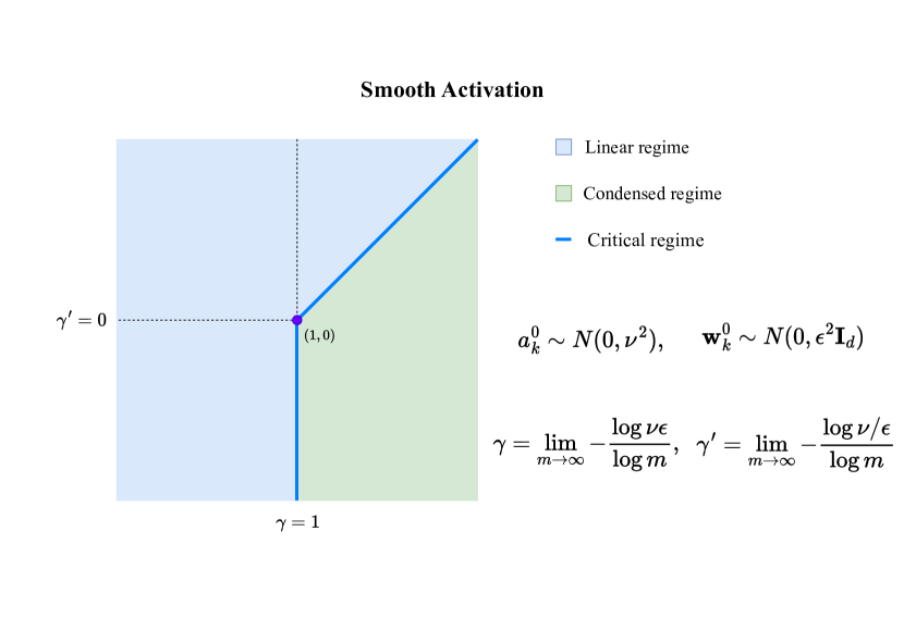
Figure 1: Phase diagram of two-layer NNs.

Firstly, we established the phase diagram of initial condensation for two-layer neural networks (NNs) with a wide class of smooth activation functions, as illustrated Figure 1. Note that the phase diagram drawn in [16] is only for two-layer wide ReLU networks and the phase diagram in [32] is empirical for three-layer wide ReLU networks. The phase diagram of a two-layer neural network refers to a graphical representation of the dynamical behavior of the network as a function of its initialization scales. In this diagram, different regions correspond to different types of behaviors exhibited by NNs, such as the linear regime, where the network behaves like a linear model, and the condensed regime, where the network exhibits the initial condensation phenomenon.

Secondly, we reveal the mechanism of initial condensation for two-layer NNs and identify the directions towards which the weight parameters condense. There has been a flurry of recent papers endeavor to analyze the mechanism underlying the condensation of NNs at the initial training stage under small initialization  [18, 21, 16, 17, 32]. For instance, Maennel et al. [18] uncovered that for two-layer ReLU NNs, the GF limits the weight vectors to a certain number of directions depending sorely on the input data. Zhou et al. [32] showed empirically that condensation is a common feature in non-linear training regime for three-layer ReLU NNs. Theoretically, Maennel et al. [18] argued that GF prefers “simple” functions over “complex” ones, and Zhou et. al. [31] demonstrated that the maximal number of condensed orientations at initial training stage is twice the multiplicity (Definition 1) of the activation function. However, these proofs are heuristic as they do not account for the dynamics of parameters. Pellegrini and Biroli [21] derived a mean-field model demonstrating that two-layer ReLU NNs, when trained with hinge loss and infinite data, lead to a linear classifier. Nonetheless, their analysis does not illustrate how the initial condensation depends on the scale of initialization and does not specify which directions NNs condense on.

The organization of the paper is listed as follows. In Section 2, we discuss some related works. In Section 3, we give some preliminary introduction to our problems. In Section 4, we state our main results and show some empirical evidence. In Section 5, we give out the outline of proofs for our main results, and conclusions are drawn in Section 6. All the details of the proof are deferred to the Appendix.

2 Related Works

There has been a rich literature on the choice of initialization schemes in order to facilitate neural network training [7, 9, 19, 24], and most of the work identified the width $m$ as a hyperparameter, where the kernel regime is reached when the width grows towards infinity [11, 27, 6]. However, with the introduction of lazy training by Chizat et al. [4], instead of the width $m$, one shall take the initialization scale as the relevant hyperparameter. The lazy training refers to the phenomenon in which a heavily over-parameterized NN trained with gradient-based methods could converge exponentially fast to zero training loss with its parameters hardly varying, and such phenomenon can be observed in any non-convex model accompanied by the choice of an appropriate scaling factor of the initialization. Follow-up work by Woodworth et al. [26] focus on how the scale of initialization acts as a controlling quantity for the transition between two very different regimes, namely the kernel regime and the rich regime, for the matrix factorization problems. As for two-layer ReLU NNs, the phase digram in Luo et al. [16] identified three regimes, namely the linear regime, the critical regime and the condensed regime, based on the relative change of input weights as the width $m$ approaches infinity. In summary, the selection of appropriate initialization scales plays a crucial role in the training of NNs.

Several theoretical works studying the dynamical behavior of NNs with small initialization can be connected to implicit regularization effect provided by the weight initialization schemes, and the condensation phenomenon has also been studied under different names. Ji and Telgarsky [12] analyzed the implicit regularization of GF on deep linear networks and observed the matrix alignment phenomena, i.e., weight matrices belonging to different layers share the same direction. The weight quantization effect [18] in training two-layer ReLU NNs with small initialization is really the condensation phenomenon in disguise, and so is the case for the weight cluster effect [2] in learning the MNIST task for a three-layer CNN. Luo et al. [16] focused on how the condensation phenomenon can be clearly detected by the choice of initialization schemes, but they did not show the reason behind it. Zhang et al. [28, 30] proposed a general Embedding Principle of loss landscape of DNNs, showing that a larger DNN can experience critical points with condensed parameter, and its output is the same as that of a much smaller DNN, but their analysis did not involve its dynamical behavior. Zhou et al. [31] presented a theory for the initial direction towards which the weight vector condenses, yet it is far from satisfactory.

3 Preliminaries

3.1 Notations

We begin this section by introducing some notations that will be used in the rest of this paper. We set $n$ for the number of input samples and $m$ for the width of the neural network. We set $\mathcal{N}(\bm{\mu},\Sigma)$ as the normal distribution with mean $\bm{\mu}$ and covariance $\Sigma$. We let $[n]=\{1,2,\ldots,n\}$. We denote vector $L^{2}$ norm as $\left\lVert\cdot\right\rVert_{2}$, vector or function $L_{\infty}$ norm as $\left\lVert\cdot\right\rVert_{\infty}$, matrix spectral (operator) norm as $\left\lVert\cdot\right\rVert_{2\to 2}$, matrix infinity norm as $\left\lVert\cdot\right\rVert_{\infty\to\infty}$, and matrix Frobenius norm as $\left\lVert\cdot\right\rVert_{\mathrm{F}}.$ For a matrix $\mathbf{A}$, we use $\mathbf{A}_{i,j}$ to denote its $(i,j)$-th entry. We will also use $\mathbf{A}_{i,\text{ : }}$ to denote the $i$-th row vector of $\mathbf{A}$ and define $\mathbf{A}_{i,j:k}=$ $\left[\mathbf{A}_{i,j},\mathbf{A}_{i,j+1},\cdots,\mathbf{A}_{i,k}\right]^{\intercal}$ as part of the vector. Similarly, $\mathbf{A}_{:,i}$ is the $i$-th column vector and $\mathbf{A}_{j:k,i}$ is a part of the $i$-th column vector. For a semi-positive-definite matrix $\bm{A},$ we denote its smallest eigenvalue by $\lambda_{\min}(\bm{A}),$ and correspondingly, its largest eigenvalue by $\lambda_{\max}(\bm{A})$. We use $\mathcal{O}(\cdot)$ and $\Omega(\cdot)$ for the standard Big-O and Big-Omega notations. We finally denote the set of continuous functions $f(\cdot):\mathbb{R}\to\mathbb{R}$ possessing continuous derivatives of order up to and including $r$ by $\mathcal{C}^{r}(\mathbb{R})$, the set of analytic functions $f(\cdot):\mathbb{R}\to\mathbb{R}$ by $\mathcal{C}^{\omega}(\mathbb{R})$, and $\left<\cdot,\cdot\right>$ for standard inner product between two vectors.

3.2 Problem Setup

We use almost the same settings in Luo et al. [16] by starting with the original model

$$f_{\bm{\theta}}(\bm{x})=\sum_{k=1}^{m}a_{k}\sigma(\bm{w}_{k}^{\intercal}\bm{x}),$$ (3.1)

whose parameters $\bm{\theta}^{0}:=\mathrm{vec}(\bm{\theta}_{a}^{0},\bm{\theta}_{\bm{w}}^{0})$ are initialized by

$$a_{k}^{0}\sim\mathcal{N}(0,\nu^{2}),\quad\bm{w}_{k}^{0}\sim\mathcal{N}(\bm{0},\varepsilon^{2}\bm{I}_{d}),$$ (3.2)

and the empirical risk is

$$R_{S}(\bm{\theta})=\frac{1}{2n}\sum_{i=1}^{n}{(f_{\bm{\theta}}(\bm{x}_{i})-y_{i})}^{2}.$$ (3.3)

Then the training dynamics based on gradient descent (GD) at the continuous limit obeys the following gradient flow precisely reads: For $k\in[m]$,

$$\frac{\mathrm{d}a_{k}}{\mathrm{d}t} =-\frac{1}{n}\sum_{i=1}^{n}\left(\sum_{k^{\prime}=1}^{m}{a}_{k^{\prime}}{\sigma({\bm{w}}_{k^{\prime}}^{\intercal}\bm{x}_{i})}-y_{i}\right)\sigma(\bm{w}_{k}^{\intercal}\bm{x}_{i}),$$ (3.4)

$$\frac{\mathrm{d}\bm{w}_{k}}{\mathrm{d}t} =-\frac{1}{n}\sum_{i=1}^{n}\left(\sum_{k^{\prime}=1}^{m}{a}_{k^{\prime}}{\sigma({\bm{w}}_{k^{\prime}}^{\intercal}\bm{x}_{i})}-y_{i}\right)a_{k}\sigma^{(1)}(\bm{w}_{k}^{\intercal}\bm{x}_{i})\bm{x}_{i}.$$

We identify the parameters $\bm{\theta}_{a}:=\mathrm{vec}(\{a_{k}\}_{k=1}^{m})$ and $\bm{\theta}_{\bm{w}}:=\mathrm{vec}(\{\bm{w}_{k}\}_{k=1}^{m})$ as variables of order one by setting

$$a_{k}=\nu\bar{a}_{k},\quad\bm{w}_{k}=\varepsilon\bar{\bm{w}}_{k},$$

then the rescaled dynamics can be written as

$$\nu\frac{\mathrm{d}\bar{a}_{k}}{\mathrm{d}{t}} =-\frac{1}{n}\sum_{i=1}^{n}\left(\sum_{k^{\prime}=1}^{m}\nu\varepsilon\bar{a}_{k^{\prime}}\frac{\sigma(\varepsilon\bar{\bm{w}}_{k^{\prime}}^{\intercal}\bm{x}_{i})}{\varepsilon}-y_{i}\right)\varepsilon\frac{\sigma(\varepsilon\bar{\bm{w}}_{k}^{\intercal}\bm{x}_{i})}{\varepsilon},$$ (3.5)

$$\varepsilon\frac{\mathrm{d}\bar{\bm{w}}_{k}}{\mathrm{d}{t}} =-\frac{1}{n}\sum_{i=1}^{n}\left(\sum_{k^{\prime}=1}^{m}\nu\varepsilon\bar{a}_{k^{\prime}}\frac{\sigma(\varepsilon\bar{\bm{w}}_{k^{\prime}}^{\intercal}\bm{x}_{i})}{\varepsilon}-y_{i}\right)\nu\bar{a}_{k}\sigma^{(1)}(\varepsilon\bar{\bm{w}}_{k}^{\intercal}\bm{x}_{i})\bm{x}_{i}.$$

For the case where $\varepsilon\ll 1$ and $\varepsilon\gg 1$, the expressions $\frac{\sigma(\varepsilon\bar{\bm{w}}_{k}^{\intercal}\bm{x}_{i})}{\varepsilon}$ and ${\sigma^{(1)}(\varepsilon\bar{\bm{w}}_{k}^{\intercal}\bm{x}_{i})}$ are hard to handle at first glance. However, in the case where $\varepsilon\ll 1$, under the condition (1) that $\sigma(0)=0$ and $\sigma^{(1)}(0)=1$, we obtain that

$$\frac{\sigma(\varepsilon\bar{\bm{w}}_{k}^{\intercal}\bm{x}_{i})}{\varepsilon}\approx\bar{\bm{w}}_{k}^{\intercal}\bm{x}_{i},\quad{\sigma^{(1)}(\varepsilon\bar{\bm{w}}_{k}^{\intercal}\bm{x}_{i})}\approx 1,$$

hence $\frac{\sigma(\varepsilon\bar{\bm{w}}_{k}^{\intercal}\bm{x}_{i})}{\varepsilon}$ and ${\sigma^{(1)}(\varepsilon\bar{\bm{w}}_{k}^{\intercal}\bm{x}_{i})}$ are of order one.

In the case where $\varepsilon\gg 1$, under the condition (2) that

$$\lim_{x\to-\infty}{\sigma^{(1)}(x)}=a,\quad\lim_{x\to+\infty}{\sigma^{(1)}(x)}=b,$$

we obtain that

$$\frac{\sigma(\varepsilon\bar{\bm{w}}_{k}^{\intercal}\bm{x}_{i})}{\varepsilon}\approx\sigma^{(1)}(\varepsilon\bar{\bm{w}}_{k}^{\intercal}\bm{x}_{i}),$$

hence $\frac{\sigma(\varepsilon\bar{\bm{w}}_{k}^{\intercal}\bm{x}_{i})}{\varepsilon}$ and ${\sigma^{(1)}(\varepsilon\bar{\bm{w}}_{k}^{\intercal}\bm{x}_{i})}$ are also of order one. Under these two aforementioned conditions, $\sigma(\cdot)$ acts like a linear activation in the case where $\varepsilon\ll 1$, and acts like a leaky-ReLU activation activation in the case where $\varepsilon\gg 1$, both of which are homogeneous functions. Hence the above dynamics can be simplified into

$$\frac{\mathrm{d}\bar{a}_{k}}{\mathrm{d}{t}} =-\frac{1}{n}\sum_{i=1}^{n}\left(\sum_{k^{\prime}=1}^{m}\nu\varepsilon\bar{a}_{k^{\prime}}\frac{\sigma(\varepsilon\bar{\bm{w}}_{k^{\prime}}^{\intercal}\bm{x}_{i})}{\varepsilon}-y_{i}\right)\frac{\varepsilon}{\nu}\frac{\sigma(\varepsilon\bar{\bm{w}}_{k}^{\intercal}\bm{x}_{i})}{\varepsilon},$$ (3.6)

$$\frac{\mathrm{d}\bar{\bm{w}}_{k}}{\mathrm{d}{t}} =-\frac{1}{n}\sum_{i=1}^{n}\left(\sum_{k^{\prime}=1}^{m}\nu\varepsilon\bar{a}_{k^{\prime}}\frac{\sigma(\varepsilon\bar{\bm{w}}_{k^{\prime}}^{\intercal}\bm{x}_{i})}{\varepsilon}-y_{i}\right)\frac{\nu}{\varepsilon}\bar{a}_{k}\sigma^{(1)}(\varepsilon\bar{\bm{w}}_{k}^{\intercal}\bm{x}_{i})\bm{x}_{i}.$$

We hereby introduce two scaling parameters

$$\kappa:={\nu\varepsilon},\quad\kappa^{\prime}:=\frac{\nu}{\varepsilon},$$ (3.7)

then the dynamics (3.6) can be written as a normalized flow

$$\frac{\mathrm{d}\bar{a}_{k}}{\mathrm{d}{t}} =-\frac{1}{n}\sum_{i=1}^{n}\left(\sum_{k^{\prime}=1}^{m}\kappa\bar{a}_{k^{\prime}}\frac{\sigma(\varepsilon\bar{\bm{w}}_{k^{\prime}}^{\intercal}\bm{x}_{i})}{\varepsilon}-y_{i}\right)\frac{1}{\kappa^{\prime}}\frac{\sigma(\varepsilon\bar{\bm{w}}_{k}^{\intercal}\bm{x}_{i})}{\varepsilon},$$ (3.8)

$$\frac{\mathrm{d}\bar{\bm{w}}_{k}}{\mathrm{d}{t}} =-\frac{1}{n}\sum_{i=1}^{n}\left(\sum_{k^{\prime}=1}^{m}\kappa\bar{a}_{k^{\prime}}\frac{\sigma(\varepsilon\bar{\bm{w}}_{k^{\prime}}^{\intercal}\bm{x}_{i})}{\varepsilon}-y_{i}\right)\kappa^{\prime}\bar{a}_{k}\sigma^{(1)}(\varepsilon\bar{\bm{w}}_{k}^{\intercal}\bm{x}_{i})\bm{x}_{i}.$$

with the following initialization

$$\bar{a}_{k}^{0}\sim\mathcal{N}(0,1),\quad\bar{\bm{w}}_{k}^{0}\sim\mathcal{N}(\bm{0},\bm{I}_{d}).$$ (3.9)

In the following discussion throughout this paper, we always refer to this rescaled model (3.8) and drop all the “bar”s of $\{a_{k}\}_{k=1}^{m}$ and $\{\bm{w}_{k}\}_{k=1}^{m}$ for notational simplicity.

As $\kappa$ and $\kappa^{\prime}$ are always in specific power-law relations to the width $m$, we introduce two independent coordinates

$$\gamma:=\lim_{m\to\infty}-\frac{\log\kappa}{\log m},\quad\gamma^{\prime}:=\lim_{m\to\infty}-\frac{\log\kappa^{\prime}}{\log m},$$ (3.10)

which meet all the guiding principles [16] for finding the coordinates of a phase diagram.

Before we end this section, we list out some commonly-used initialization methods with their scaling parameters as shown in Table 1.

Name	$\nu$	$\varepsilon$	$\kappa~{}(\nu\varepsilon)$	$\kappa^{\prime}~{}({\nu}/{\varepsilon})$	$\gamma$	$\gamma^{\prime}$
LeCun [14]	$\sqrt{\frac{1}{m}}$	$\sqrt{\frac{1}{d}}$	$\sqrt{\frac{1}{md}}$	$\sqrt{\frac{d}{m}}$	$\frac{1}{2}$	$\frac{1}{2}$
He [8]	$\sqrt{\frac{2}{m}}$	$\sqrt{\frac{2}{d}}$	$\sqrt{\frac{4}{md}}$	$\sqrt{\frac{d}{m}}$	$\frac{1}{2}$	$\frac{1}{2}$
Xavier [7]	$\sqrt{\frac{2}{m+1}}$	$\sqrt{\frac{2}{m+d}}$	$\sqrt{\frac{4}{(m+1)(d+1)}}$	$\sqrt{\frac{m+d}{m+1}}$	$1$	$0$
Huang [10]	$1$	$\sqrt{\frac{1}{m}}$	$\sqrt{\frac{1}{m}}$	$\sqrt{m}$	$\frac{1}{2}$	$-\frac{1}{2}$

Table 1: Initialization methods with their scaling parameters

4 Main Results

4.1 Activation function and input

In this part, we shall impose some technical conditions on the activation function and input samples. We start with a technical condition [31, Definition 1] on the activation function $\sigma(\cdot)$

Definition 1 (Multiplicity $p$).

$\sigma(\cdot):\mathbb{R}\to\mathbb{R}$ has multiplicity $p$ if there exists an integer $p\geq 1$, such that for all $0\leq s\leq p-1$, the $s$-th order derivative satisfies $\sigma^{(s)}(0)=0$, and $\sigma^{(p)}(0)\neq 0$.

We list out some examples of activation functions with different multiplicity.

Remark 1.

• $tanh(x):=\frac{\exp(x)-\exp(-x)}{\exp(x)+\exp(-x)}$ is with multiplicity $p=1$;
  

• $SiLU(x):=\frac{x}{1+\exp(-x)}$ is with multiplicity $p=1$;
  

• $xtanh(x):=\frac{x\exp(x)-x\exp(-x)}{\exp(x)+\exp(-x)}$ is with multiplicity $p=2$.

Assumption 1 (Multiplicity $1$).

The activation function $\sigma\in\mathcal{C}^{2}(\mathbb{R})$, and there exists a universal constant $C_{L}>0$, such that its first and second derivatives satisfy

$$\left\lVert\sigma^{(1)}(\cdot)\right\rVert_{\infty}\leq C_{L},\quad\left\lVert\sigma^{(2)}(\cdot)\right\rVert_{\infty}\leq C_{L}.$$ (4.1)

Moreover,

$$\sigma(0)=0,\quad\sigma^{(1)}(0)=1.$$ (4.2)

Remark 2.

We remark that $\sigma$ has multiplicity $1$. $\sigma^{(1)}(0)=1$ can be replaced by $\sigma^{(1)}(0)\neq 0$, and we set $\sigma^{(1)}(0)=1$ for simplicity, and it can be easily satisfied by replacing the original activation $\sigma(\cdot)$ with $\frac{\sigma(\cdot)}{\sigma^{(1)}(0)}$.

We note that 1 can be satisfied by using the tanh activation:

$$\sigma(x)=\frac{\exp(x)-\exp(-x)}{\exp(x)+\exp(-x)},$$

and the scaled SiLU activation

$$\sigma(x)=\frac{2x}{1+\exp(-x)}.$$

Assumption 2.

The activation function $\sigma\in\mathcal{C}^{\omega}(\mathbb{R})$ and is not a polynomial function, also its function value at $0$ satisfy

$${\sigma(0)}=0,$$ (4.3)

also there exists a universal constant $C_{L}>0$, such that its first and second derivatives satisfy

$${\sigma^{(1)}(0)}=1,\quad\left\lVert\sigma^{(1)}(\cdot)\right\rVert_{\infty}\leq C_{L},\quad\left\lVert\sigma^{(2)}(\cdot)\right\rVert_{\infty}\leq C_{L}.$$ (4.4)

Moreover,

$$\lim_{x\to-\infty}{\sigma^{(1)}(x)}=a,\quad\lim_{x\to+\infty}{\sigma^{(1)}(x)}=b,$$ (4.5)

and $a\neq b$.

Remark 3.

We note that 2 can be satisfied by by using the scaled SiLU activation:

$$\sigma(x)=\frac{2x}{1+\exp(-x)},$$

where $a=0$ and $b=2$.

Some other functions also satisfy this assumption, for instance, the modified scaled softplus activation:

$$\sigma(x)=2\left(\log(1+\exp(x))-\log 2\right),$$

where $a=0$ and $b=2$.

Assumption 3 (Non-degenerate data).

The training inputs and labels $\mathcal{S}=\{(\bm{x}_{i},y_{i})\}_{i=1}^{n}$ satisfy that there exists a universal constant $c>0$, such that for all $i\in[n]$,

$$\frac{1}{c}\leq\left\lVert\bm{x}_{i}\right\rVert_{2},\quad\left\lvert y_{i}\right\rvert\leq c,$$

and

$$\sum_{i=1}^{n}y_{i}{\bm{x}}_{i}\neq\mathbf{0}.$$ (4.6)

We denote by

$$\bm{z}:=\frac{1}{n}\sum_{i=1}^{n}y_{i}{\bm{x}}_{i},$$ (4.7)

and assume further that for some universal constant $c>0$, the following holds

$$\frac{1}{c}\leq\left\lVert\bm{z}\right\rVert_{2}\leq c,$$ (4.8)

and its unit vector

$$\hat{\bm{z}}:=\frac{\sum_{i=1}^{n}y_{i}{\bm{x}}_{i}}{\left\lVert\sum_{i=1}^{n}y_{i}{\bm{x}}_{i}\right\rVert_{2}}.$$ (4.9)

Assumption 4.

The training inputs and labels $\mathcal{S}=\{(\bm{x}_{i},y_{i})\}_{i=1}^{n}$ satisfy that there exists a universal constant $c>0$, such that for all $i\in[n]$,

$$\frac{1}{c}\leq\left\lVert\bm{x}_{i}\right\rVert_{2},\quad\left\lvert y_{i}\right\rvert\leq c,$$

and all training inputs are non-parallel with each other, i.e., for any $i\neq j$ and $i,j\in[n]$,

$$\bm{x}_{i}\nparallel\bm{x}_{j}.$$

We remark that the requirements in 3 are easier to meet compared with 4, and both assumptions impose the input sample $\mathcal{S}=\{(\bm{x}_{i},y_{i})\}_{i=1}^{n}$ to be of order one.

Assumption 5.

The following limit exists

$${\gamma}_{1}:=\lim_{m\to\infty}-\frac{\log\nu}{\log m},\quad{\gamma}_{2}:=\lim_{m\to\infty}-\frac{\log\varepsilon}{\log m},$$ (4.10)

then by definition

$$\gamma=\lim_{m\to\infty}-\frac{\log\nu\varepsilon}{\log m}={\gamma}_{1}+\gamma_{2},\quad\gamma^{\prime}=\lim_{m\to\infty}-\frac{\log\frac{\nu}{\varepsilon}}{\log m}={\gamma}_{1}-\gamma_{2}.$$

4.2 Regime Characterization at Initial Stage

Before presenting our theory that establishes a consistent boundary to separate the diagram into two distinct areas, namely the linear regime area and the condensed regime area, we introduce a quantity that has proven to be valuable in the analysis of NNs.

It is known that the output of a two-layer NN is linear with respect to $\bm{\theta}_{a}$, hence if the set of parameter $\bm{\theta}_{\bm{w}}$ remain stuck to its initialization throughout the whole training process, then the training dynamics of a two-layer NN can be linearized around the initialization. In the phase diagram, the linear regime area precisely corresponds to the region where the output function of a two-layer NN can be well approximated by its linearized model, i.e., in the linear regime area, the following holds

$$f_{\bm{\theta}}(\bm{x}) \approx f\left(\bm{x},\bm{\theta}(0)\right)+\left<\nabla_{\bm{\theta}_{a}}f\left(\bm{x},\bm{\theta}(0)\right),\bm{\theta}_{a}(t)-\bm{\theta}_{a}(0)\right>$$ (4.11)

$$~{}~{}~{}~{}~{}~{}~{}~{}~{}~{}~{}~{}~{}~{}~{}~{}~{}~{}+\left<\nabla_{\bm{\theta}_{\bm{w}}}f\left(\bm{x},\bm{\theta}(0)\right),\bm{\theta}_{\bm{w}}(t)-\bm{\theta}_{\bm{w}}(0)\right>.$$

In general, this linear approximation holds only when $\bm{\theta}_{\bm{w}}(t)$ remains within a small neighbourhood of $\bm{\theta}_{\bm{w}}(0)$. Since the size of this neighbourhood scales with $\lVert\bm{\theta}_{\bm{w}}(0)\rVert_{2}$, therefore we use the following quantity as an indicator of how far $\bm{\theta}_{\bm{w}}(t)$ deviates away from $\bm{\theta}_{\bm{w}}(0)$ throughout the training process

$$\sup\limits_{t\in[0,+\infty)}\mathrm{RD}(\bm{\theta}_{\bm{w}}(t))=\frac{\left\lVert\bm{\theta}_{\bm{w}}(t)-\bm{\theta}_{\bm{w}}(0)\right\rVert_{2}}{\lVert\bm{\theta}_{\bm{w}}(0)\rVert_{2}}.$$ (4.12)

We demonstrate that as $m\to\infty$, under suitable choice of the initialization scales (the blue area in Figure 1), the NN training dynamics fall into the linear regime (Theorem 1), and for large enough $m$,

$$\sup\limits_{t\in[0,+\infty)}\mathrm{RD}(\bm{\theta}_{\bm{w}}(t))\to 0.$$

We also demonstrate that under some other choices of the initialization scales (the green area in Figure 1), the NN training dynamics fall into the condensed regime (Theorem 2), where

$$\sup\limits_{t\in[0,+\infty)}\mathrm{RD}(\bm{\theta}_{\bm{w}}(t))\to+\infty,$$

and the phenomenon of condensation can be observed, and $\bm{\theta}_{\bm{w}}$ condense toward the direction of $\bm{z}$. We observe that in both cases, as $\bm{\theta}_{\bm{w}}$ deviates far away from initialization, the approximation (4.11) fails, and NN training dynamics is essentially nonlinear with respect to $\bm{\theta}_{\bm{w}}$.

Moreover, under the remaining choice of the initialization scales (the solid blue line in Figure 1), the NN training dynamics fall into the critical regime area, and we conjecture that

$$\sup\limits_{t\in[0,+\infty)}\mathrm{RD}(\bm{\theta}_{\bm{w}}(t))\to\mathcal{O}(1),$$

whose study is beyond the scope of this paper.

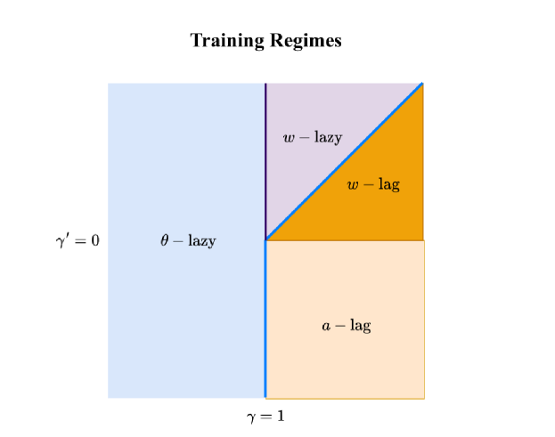
Figure 2: Different training regimes in the phase diagram.

Theorem 1 (Linear regime).

Given any $\delta\in(0,1)$, under 2, 4 and 5, if $\gamma<1$ or $\gamma^{\prime}>\gamma-1$, then with probability at least $1-\delta$ over the choice of $\bm{\theta}^{0}$,

$$\lim_{m\to\infty}\sup\limits_{t\in[0,+\infty)}\frac{\lVert\bm{\theta}_{\bm{w}}(t)-\bm{\theta}_{\bm{w}}(0)\rVert_{2}}{\lVert\bm{\theta}_{\bm{w}}(0)\rVert_{2}}=0.$$ (4.13)

Remark 4.

The linear regime area is split into two parts, one is termed the $\bm{\theta}$-lazy area (blue area in Figure 2), where $\gamma<1$, the other is termed the $\bm{w}$-lazy area (pink area in Figure 2), where $\gamma\geq 1$ and $\gamma^{\prime}>\gamma-1>0$.

In the $\bm{\theta}$-lazy area, the following relation holds

$$\lim_{m\to\infty}\sup\limits_{t\in[0,+\infty)}\frac{\lVert\bm{\theta}(t)-\bm{\theta}(0)\rVert_{2}}{\lVert\bm{\theta}(0)\rVert_{2}}=0,$$ (4.14)

whose detailed reasoning can be found in Section B.2, and in the $\bm{w}$-lazy area, relation (4.14) does not hold.

Theorem 2 (Condensed regime).

Given any $\delta\in(0,1)$, under 1, 3 and 5, if $\gamma>1$ and $\gamma^{\prime}<\gamma-1$, then with probability at least $1-\delta$ over the choice of $\bm{\theta}^{0}$, there exists $T>0$, such that

$$\lim_{m\to\infty}\sup\limits_{t\in[0,T]}\frac{\lVert\bm{\theta}_{\bm{w}}(t)-\bm{\theta}_{\bm{w}}(0)\rVert_{2}}{\lVert\bm{\theta}_{\bm{w}}(0)\rVert_{2}}=+\infty,$$ (4.15)

and

$$\lim_{m\to\infty}\sup\limits_{t\in[0,T]}\frac{\left\lVert\bm{\theta}_{\bm{w},\bm{z}}(t)\right\rVert_{2}}{\left\lVert\bm{\theta}_{\bm{w}}(t)\right\rVert_{2}}=1,$$ (4.16)

where $\bm{\theta}_{\bm{w},\bm{z}}(t):=\left[\left<\bm{w}_{1},\hat{\bm{z}}\right>,\left<\bm{w}_{2},\hat{\bm{z}}\right>,\cdots,\left<\bm{w}_{m},\hat{\bm{z}}\right>\right]^{\intercal}$.

Remark 5.

The condensed regime area is split into two parts, one is termed the $\bm{w}$-lag area (orange area in Figure 2), where $\gamma>1$ and $0\leq\gamma^{\prime}<\gamma-1$, the other is termed the $a$-lag area (yellow area in Figure 2), where $\gamma>1$ and $\gamma^{\prime}<0$.

In the $\bm{w}$-lag regime area, as illustrated in (5.14), $\bm{\theta}_{\bm{w}}$ waits for a period of time of order one until $\bm{\theta}_{a}$ attains a magnitude that is commensurate with that of $\bm{\theta}_{\bm{w}}$, and the time $T$ in Theorem 2 satisfies that

$$T\geq\log\left(\frac{1}{4}\right)+{\frac{\gamma-\gamma^{\prime}-1}{8}}\log(m),$$ (4.17)

and as $m\to\infty$, $T\to\infty$.

In the $a$-lag regime area, as illustrated in (5.14), $\bm{\theta}_{a}$ waits for a period of time of order one until $\bm{\theta}_{\bm{w}}$ attains a magnitude that is commensurate with that of $\bm{\theta}_{a}$, and it is exactly during this interval of time that the phenomenon of initial condensation can be observed. Hence for some $\alpha>0$, the time $T$ in Theorem 2 can be chosen as

$$m^{-\alpha}\leq T\leq 2m^{-\alpha},$$ (4.18)

which is obviously of order one, see Section C.4 for more details.

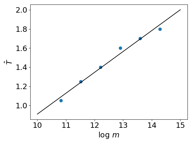
(a) $\gamma=1.4,~{}~{}R^{2}=0.983$

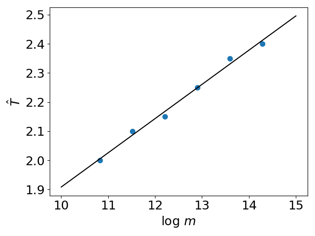
(b) $\gamma=1.6,~{}~{}R^{2}=0.991$

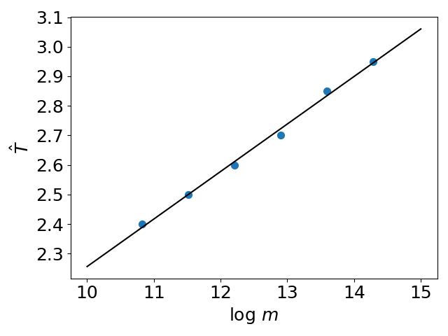
(c) $\gamma=1.8,~{}~{}R^{2}=0.995$

Figure 3: $\hat{T}$ (ordinate) vs $\log m$ (abscissa) with different values of $\gamma$ but fixed $\gamma^{\prime}=0$ for two-layer NNs with tanh activation indicated by blue dots. The black line is a linear fit, and $R^{2}$ is the coefficient of determination that provides information about the goodness of fit of a linear regression. The closer $R^{2}$ is to $1$, the better the model fits the data.

4.3 Experimental Demonstration

In order to distinguish between the $\bm{w}$-lag regime and $a$-lag regime, it is necessary to estimate the time $T$ in Remark 5, which is also a reasonale way to empirically validate our theoretical analysis. An empirical approximation of $T$ can be obtained by determining the time interval $\hat{T}$, starting from the initial stage at $t=0$, up to the point at which the quantity $\frac{\left\lVert\bm{\theta}_{\bm{w},\bm{z}}(t)\right\rVert_{2}}{\left\lVert\bm{\theta}_{\bm{w}}(t)\right\rVert_{2}}$ reaches its climax for sufficiently large values of $m$ ($m=50000,100000,200000,400000,800000,1600000$), as we are unable to run experiments at $m\to\infty$.

4.3.1 $\bm{w}$-lag regime

We validate the effectiveness of our estimates by performing a simple linear regression to visualize the relation (4.17), where $\hat{T}$ is set as the response variable and $\log m$ as the single independent variable. Figure 3 shows that NNs with different values of $\gamma$ but fixed $\gamma^{\prime}$ satisfy the relation (4.17), thereby demonstrating the accuracy and reliability of our estimates.

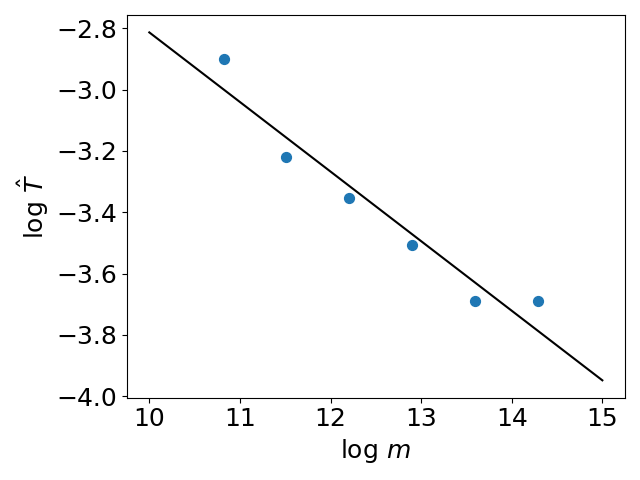
(a) $\gamma=1.2,~{}~{}R^{2}=0.936$

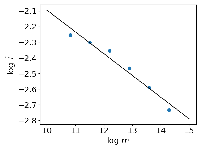
(b) $\gamma=1.4,~{}~{}R^{2}=0.977$

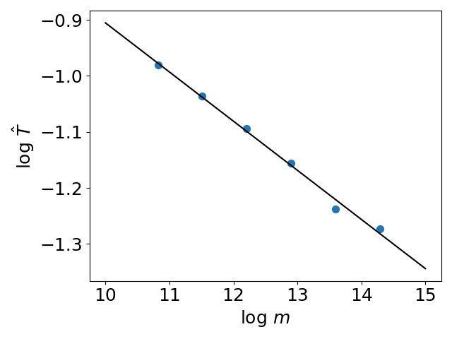
(c) $\gamma=1.6,~{}~{}R^{2}=0.993$

Figure 4: $\log\hat{T}$ (ordinate) vs $\log m$ (abscissa) with different values of $\gamma$ but fixed $\gamma^{\prime}=-0.4$ for two-layer NNs with tanh activation indicated by blue dots. The black line is a linear fit, and $R^{2}$ is the coefficient of determination.

4.3.2 $a$-lag regime

We repeat the strategy in Section 4.3.1 except that in one hand we are hereby to visualize the relation (4.18) in Figure 4, and in the other, $\log\hat{T}$ is set as the response variable and $\gamma^{\prime}$ is no longer $0$. We can still see a good agreement between the experimental data and its linear fitting, thus, validating the relation (4.18).

5 Technique Overview

In this part, we describe some technical tools and present the sketch of proofs for the above two theorems. Before we proceed, a rigorous description of the updated notations and definitions is required.

We start by a two-layer normalized NN model

$$f_{\bm{\theta}}(\bm{x})=\sum_{k=1}^{m}\nu\varepsilon a_{k}\frac{\sigma(\varepsilon\bm{w}_{k}^{\intercal}\bm{x})}{\varepsilon},$$ (5.1)

with the normalized parameters $\bm{\theta}^{0}:=\mathrm{vec}(\bm{\theta}_{a}^{0},\bm{\theta}_{\bm{w}}^{0})$ initialized by

$$a^{0}_{k} :=a_{k}(0)\sim\mathcal{N}(0,1),$$

$$\bm{w}_{k}^{0} :=\bm{w}_{k}(0)\sim\mathcal{N}(\bm{0},\bm{I}_{d}).$$

For all $i\in[n]$, we denote hereafter that

$$e_{i}:=e_{i}(\bm{\theta}):=f_{\bm{\theta}}(\bm{x}_{i})-y_{i},$$

and

$$\bm{e}:=\bm{e}(\bm{\theta}):={[e_{1}(\bm{\theta}),e_{2}(\bm{\theta}),\ldots,e_{n}(\bm{\theta})]}^{\intercal}.$$

Then the normalized flow reads: For all $k\in[m]$,

$$\frac{\mathrm{d}{a}_{k}}{\mathrm{d}{t}} =-\frac{\varepsilon}{\nu}\frac{1}{n}\sum_{i=1}^{n}e_{i}\frac{\sigma(\varepsilon{\bm{w}}_{k}^{\intercal}\bm{x}_{i})}{\varepsilon},$$ (5.2)

$$\frac{\mathrm{d}{\bm{w}}_{k}}{\mathrm{d}{t}} =-\frac{\nu}{\varepsilon}\frac{1}{n}\sum_{i=1}^{n}e_{i}{a}_{k}\sigma^{(1)}(\varepsilon{\bm{w}}_{k}^{\intercal}\bm{x}_{i})\bm{x}_{i}.$$

5.1 Linear Regime

We define the normalized kernels as follows

$$k^{[a]}(\bm{x},\bm{x}^{\prime}) :=\frac{1}{\varepsilon^{2}}\mathbb{E}_{\bm{w}}{\sigma(\varepsilon\bm{w}^{\intercal}\bm{x})\sigma(\varepsilon\bm{w}^{\intercal}\bm{x}^{\prime})},$$ (5.3)

$$k^{[\bm{w}]}(\bm{x},\bm{x}^{\prime}) :=\mathbb{E}_{(a,\bm{w})}a^{2}\sigma^{(1)}(\varepsilon\bm{w}^{\intercal}\bm{x})\sigma^{(1)}(\varepsilon\bm{w}^{\intercal}\bm{x}^{\prime})\left<\bm{x},\bm{x}^{\prime}\right>,$$

thus, the components of the Gram matrices $\bm{K}^{[a]}$ and $\bm{K}^{[\bm{w}]}$ of at infinite width respectively reads: For any $i,j\in[n]$,

$$\bm{K}^{[a]} :=\left[K_{ij}^{[a]}\right]_{n\times n},$$ (5.4)

$$K^{[a]}_{ij} :=k^{[a]}(\bm{x}_{i},\bm{x}_{j}),$$

$$\bm{K}^{[\bm{w}]} :=\left[K_{ij}^{[\bm{w}]}\right]_{n\times n},$$

$$K^{[\bm{w}]}_{ij} :=k^{[\bm{w}]}(\bm{x}_{i},\bm{x}_{j}),$$

we conclude that under 2 and 4, $\bm{K}^{[a]}$ and $\bm{K}^{[\bm{w}]}$ are strictly positive definite, and both of their least eigenvalues are of order one (Theorem 4).

We define the normalized Gram matrices $\bm{G}^{[a]}(\bm{\theta})$, $\bm{G}^{[\bm{w}]}(\bm{\theta})$, and $\bm{G}(\bm{\theta})$ for a finite width two-layer network as follows: For any $i,j\in[n]$,

$$\bm{G}^{[a]}(\bm{\theta}) :=\left[G_{ij}^{[a]}(\bm{\theta})\right]_{n\times n},$$ (5.5)

$$G^{[a]}_{ij}(\bm{\theta}) :=\frac{1}{m}\sum_{k=1}^{m}\left<\nabla_{a_{k}}f_{\bm{\theta}}(\bm{x}_{i}),\frac{\varepsilon}{\nu}\nabla_{a_{k}}f_{\bm{\theta}}(\bm{x}_{j})\right>$$

$$=\frac{\nu^{2}}{m}\frac{\varepsilon}{\nu}\sum_{k=1}^{m}\sigma(\varepsilon\bm{w}_{k}^{\intercal}\bm{x}_{i})\sigma(\varepsilon\bm{w}_{k}^{\intercal}\bm{x}_{j})$$

$$=\frac{\nu\varepsilon^{3}}{m}\sum_{k=1}^{m}\frac{1}{\varepsilon^{2}}\sigma(\varepsilon\bm{w}_{k}^{\intercal}\bm{x}_{i})\sigma(\varepsilon\bm{w}_{k}^{\intercal}\bm{x}_{j}),$$

$$\bm{G}^{[\bm{w}]}(\bm{\theta}) :=\left[G_{ij}^{[\bm{w}]}(\bm{\theta})\right]_{n\times n},$$

$$G^{[\bm{w}]}_{ij}(\bm{\theta}) :=\frac{1}{m}\sum_{k=1}^{m}\left<\nabla_{\bm{w}_{k}}f_{\bm{\theta}}(\bm{x}_{i}),\frac{\nu}{\varepsilon}\nabla_{\bm{w}_{k}}f_{\bm{\theta}}(\bm{x}_{j})\right>$$

$$=\frac{\nu^{3}\varepsilon}{m}\sum_{k=1}^{m}a_{k}^{2}\sigma^{(1)}(\varepsilon\bm{w}_{k}^{\intercal}\bm{x}_{i})\sigma^{(1)}(\varepsilon\bm{w}_{k}^{\intercal}\bm{x}_{j})\left<\bm{x}_{i},\bm{x}_{j}\right>,$$

and

$$\bm{G}(\bm{\theta}):=\bm{G}^{[a]}(\bm{\theta})+\bm{G}^{[\bm{w}]}(\bm{\theta}).$$ (5.6)

Remark 6.

We conclude that

$$\lambda_{\min}\left(\bm{G}^{[a]}\left(\bm{\theta}^{0}\right)\right)\sim\Omega(\nu\varepsilon^{3}),\quad\lambda_{\min}\left(\bm{G}^{[\bm{w}]}\left(\bm{\theta}^{0}\right)\right)\sim\Omega(\nu^{3}\varepsilon),$$ (5.7)

and it has been rigorously achieved by Proposition 2 located in Section B.1.

Finally, we obtain that

$$\frac{\mathrm{d}}{\mathrm{d}t}R_{S}(\bm{\theta}) =-\left(\sum_{k=1}^{m}\frac{\varepsilon}{\nu}\left<\nabla_{a_{k}}R_{S}(\bm{\theta}),\nabla_{a_{k}}R_{S}(\bm{\theta})\right>+\sum_{k=1}^{m}\frac{\nu}{\varepsilon}\left<\nabla_{\bm{w}_{k}}R_{S}(\bm{\theta}),\nabla_{\bm{w}_{k}}R_{S}(\bm{\theta})\right>\right)$$

$$=-\frac{m}{n^{2}}\bm{e}^{\intercal}\left(\bm{G}^{[a]}(\bm{\theta})+\bm{G}^{[\bm{w}]}(\bm{\theta})\right)\bm{e}.$$

In the case where $\gamma<1$ ($\bm{\theta}$-lazy regime), the following holds for all $t>0$:

$$\lambda_{\min}\left(\bm{G}^{[a]}(\bm{\theta}(t))\right)\geq\frac{1}{2}\nu\varepsilon^{3}\lambda,\quad\lambda_{\min}\left(\bm{G}^{[\bm{w}]}(\bm{\theta}(t))\right)\geq\frac{1}{2}\nu^{3}\varepsilon\lambda,$$

for some universal constant $\lambda>0$. Hence, we obtain that

$$\frac{\mathrm{d}}{\mathrm{d}t}R_{S}(\bm{\theta}(t)) =-\frac{m}{n^{2}}\bm{e}^{\intercal}\left(\bm{G}^{[a]}(\bm{\theta}(t))+\bm{G}^{[\bm{w}]}(\bm{\theta}(t))\right)\bm{e}$$

$$\leq-\frac{2m}{n}\lambda_{\min}\left(\bm{G}(\bm{\theta}(t))\right)R_{S}(\bm{\theta}(t))$$

$$\leq-\frac{m}{n}\nu^{2}\varepsilon^{2}\left(\frac{\varepsilon}{\nu}\lambda+\frac{\nu}{\varepsilon}\lambda\right)R_{S}(\bm{\theta}(t)),$$

then

$$R_{S}(\bm{\theta}(t))\leq\exp\left(-\frac{m}{n}\nu^{2}\varepsilon^{2}\left(\frac{\varepsilon}{\nu}\lambda+\frac{\nu}{\varepsilon}\lambda\right)t\right)R_{S}(\bm{\theta}(0)).$$ (5.8)

The following relation

$$\lim_{m\to\infty}\sup\limits_{t\in[0,+\infty)}\frac{\lVert\bm{\theta}(t)-\bm{\theta}(0)\rVert_{2}}{\lVert\bm{\theta}(0)\rVert_{2}}=0,$$ (5.9)

is illustrated through an intuitive scaling analysis. Since

$$\frac{\mathrm{d}}{\mathrm{d}t}R_{S}(\bm{\theta}(t))=-\frac{\varepsilon}{\nu}\left\lVert\nabla_{\bm{\theta}_{a}}R_{S}(\bm{\theta}(t))\right\rVert_{2}^{2}-\frac{\nu}{\varepsilon}\left\lVert\nabla_{\bm{\theta}_{\bm{w}}}R_{S}(\bm{\theta}(t))\right\rVert_{2}^{2}\sim-\frac{m}{n}\nu^{2}\varepsilon^{2}\left(\frac{\varepsilon}{\nu}\lambda+\frac{\nu}{\varepsilon}\lambda\right)R_{S}(\bm{\theta}(t)),$$

then we have that

$$R_{S}(\bm{\theta}(t))\sim\exp\left(-{\frac{m}{n}\nu^{2}\varepsilon^{2}\left(\frac{\varepsilon}{\nu}\lambda+\frac{\nu}{\varepsilon}\lambda\right)}t\right){R_{S}(\bm{\theta}(0))},$$

and

$$\left\lVert\nabla_{\bm{\theta}_{a}}R_{S}(\bm{\theta}(t))\right\rVert_{2} \sim\sqrt{\frac{m}{n}\nu^{3}\varepsilon\left(\frac{\varepsilon}{\nu}\lambda+\frac{\nu}{\varepsilon}\lambda\right)}\sqrt{R_{S}(\bm{\theta}(t))}$$

$$\sim\sqrt{\frac{m}{n}\nu^{3}\varepsilon\left(\frac{\varepsilon}{\nu}\lambda+\frac{\nu}{\varepsilon}\lambda\right)}\exp\left(-{\frac{m}{2n}\nu^{2}\varepsilon^{2}\left(\frac{\varepsilon}{\nu}\lambda+\frac{\nu}{\varepsilon}\lambda\right)}t\right)\sqrt{R_{S}(\bm{\theta}(0))},$$

$$\left\lVert\nabla_{\bm{\theta}_{\bm{w}}}R_{S}(\bm{\theta}(t))\right\rVert_{2} \sim\sqrt{\frac{m}{n}\nu\varepsilon^{3}\left(\frac{\varepsilon}{\nu}\lambda+\frac{\nu}{\varepsilon}\lambda\right)}\sqrt{R_{S}(\bm{\theta}(t))}$$

$$\sim\sqrt{\frac{m}{n}\nu\varepsilon^{3}\left(\frac{\varepsilon}{\nu}\lambda+\frac{\nu}{\varepsilon}\lambda\right)}\exp\left(-{\frac{m}{2n}\nu^{2}\varepsilon^{2}\left(\frac{\varepsilon}{\nu}\lambda+\frac{\nu}{\varepsilon}\lambda\right)}t\right)\sqrt{R_{S}(\bm{\theta}(0))},$$

both holds, hence

$${\lVert\bm{\theta}(t)-\bm{\theta}(0)\rVert_{2}} \leq{\lVert\bm{\theta}_{a}(t)-\bm{\theta}_{a}(0)\rVert_{2}}+{\lVert\bm{\theta}_{\bm{w}}(t)-\bm{\theta}_{\bm{w}}(0)\rVert_{2}}$$

$$\leq\frac{\varepsilon}{\nu}\int_{0}^{t}\left\lVert\nabla_{\bm{\theta}_{a}}R_{S}(\bm{\theta}(s))\right\rVert_{2}\mathrm{d}s+\frac{\nu}{\varepsilon}\int_{0}^{t}\left\lVert\nabla_{\bm{\theta}_{\bm{w}}}R_{S}(\bm{\theta}(s))\right\rVert_{2}\mathrm{d}s$$

$$\leq\frac{\varepsilon}{\nu}\int_{0}^{\infty}\left\lVert\nabla_{\bm{\theta}_{a}}R_{S}(\bm{\theta}(s))\right\rVert_{2}\mathrm{d}s+\frac{\nu}{\varepsilon}\int_{0}^{\infty}\left\lVert\nabla_{\bm{\theta}_{\bm{w}}}R_{S}(\bm{\theta}(s))\right\rVert_{2}\mathrm{d}s$$

$$\lesssim\left(\sqrt{\frac{\varepsilon}{\nu}}+\sqrt{\frac{\nu}{\varepsilon}}\right)\sqrt{\frac{n}{{m}\nu^{2}\varepsilon^{2}\left(\frac{\varepsilon}{\nu}\lambda+\frac{\nu}{\varepsilon}\lambda\right)}}\sqrt{R_{S}(\bm{\theta}(0))},$$

and

$$\left\lVert\bm{\theta}(0)\right\rVert_{2}\sim\sqrt{m},$$

hence

$$\frac{{\lVert\bm{\theta}(t)-\bm{\theta}(0)\rVert_{2}}}{\left\lVert\bm{\theta}(0)\right\rVert_{2}} \lesssim\left(\sqrt{\frac{\varepsilon}{\nu}}+\sqrt{\frac{\nu}{\varepsilon}}\right)\sqrt{\frac{n}{{m}^{2}\nu^{2}\varepsilon^{2}\left(\frac{\varepsilon}{\nu}\lambda+\frac{\nu}{\varepsilon}\lambda\right)}}\sqrt{R_{S}(\bm{\theta}(0))}$$ (5.10)

$$\lesssim\sqrt{\frac{n}{{m}^{2}\nu^{2}\varepsilon^{2}}}\sqrt{R_{S}(\bm{\theta}(0))}.$$

The rigorous statements of relations (5.8) and (5.9) are given in Theorem 5.

In the case where $\gamma\geq 1$ and $\gamma^{\prime}>\gamma-1$ ($\bm{w}$-lazy regime), the following holds for all $t>0$:

$$\lambda_{\min}\left(\bm{G}^{[a]}(\bm{\theta}(t))\right)\geq\frac{1}{2}\nu\varepsilon^{3}\lambda,$$

for some universal constant $\lambda>0$. Hence, we have

$$\frac{\mathrm{d}}{\mathrm{d}t}R_{S}(\bm{\theta}(t)) =-\frac{m}{n^{2}}\bm{e}^{\intercal}\left(\bm{G}^{[a]}(\bm{\theta}(t))+\bm{G}^{[\bm{w}]}(\bm{\theta}(t))\right)\bm{e}$$

$$\leq-\frac{2m}{n}\lambda_{\min}\left(\bm{G}^{[a]}(\bm{\theta}(t))\right)R_{S}(\bm{\theta}(t))$$

$$\leq-\frac{m}{n}\nu^{2}\varepsilon^{2}\frac{\varepsilon}{\nu}\lambda R_{S}(\bm{\theta}(t))$$

$$=-\frac{m}{n}\nu\varepsilon^{3}\lambda R_{S}(\bm{\theta}(t)),$$

thus the following holds

$$R_{S}(\bm{\theta}(t))\leq\exp\left(-\frac{m\nu\varepsilon^{3}\lambda t}{n}\right)R_{S}(\bm{\theta}(0)),$$

and (5.9) does not hold anymore. However, we still have

$$\lim_{m\to\infty}\sup\limits_{t\in[0,+\infty)}\frac{\lVert\bm{\theta}_{\bm{w}}(t)-\bm{\theta}_{\bm{w}}(0)\rVert_{2}}{\lVert\bm{\theta}_{\bm{w}}(0)\rVert_{2}}=0,$$ (5.11)

and it can also be illustrated through an intuitive scaling analysis. Since

$$\frac{\mathrm{d}}{\mathrm{d}t}R_{S}(\bm{\theta}(t))=-\frac{\varepsilon}{\nu}\left\lVert\nabla_{\bm{\theta}_{a}}R_{S}(\bm{\theta}(t))\right\rVert_{2}^{2}-\frac{\nu}{\varepsilon}\left\lVert\nabla_{\bm{\theta}_{\bm{w}}}R_{S}(\bm{\theta}(t))\right\rVert_{2}^{2}\sim-\frac{m}{n}\nu\varepsilon^{3}\lambda R_{S}(\bm{\theta}(t)),$$

then

$$\left\lVert\nabla_{\bm{\theta}_{\bm{w}}}R_{S}(\bm{\theta}(t))\right\rVert_{2} \sim\sqrt{\frac{m}{n}\varepsilon^{4}\lambda}\sqrt{R_{S}(\bm{\theta}(t))}$$

$$\sim\sqrt{\frac{m}{n}\varepsilon^{4}\lambda}\exp\left(-\frac{m\nu\varepsilon^{3}\lambda t}{2n}\right)\sqrt{R_{S}(\bm{\theta}(0))},$$

hence

$${\lVert\bm{\theta}_{\bm{w}}(t)-\bm{\theta}_{\bm{w}}(0)\rVert_{2}} \leq\frac{\nu}{\varepsilon}\int_{0}^{t}\left\lVert\nabla_{\bm{\theta}_{\bm{w}}}R_{S}(\bm{\theta}(s))\right\rVert_{2}\mathrm{d}s$$

$$\leq\frac{\nu}{\varepsilon}\int_{0}^{\infty}\left\lVert\nabla_{\bm{\theta}_{\bm{w}}}R_{S}(\bm{\theta}(s))\right\rVert_{2}\mathrm{d}s$$

$$\lesssim\sqrt{\frac{n}{{m}\varepsilon^{4}\lambda}}\sqrt{R_{S}(\bm{\theta}(0))},$$

and as

$$\left\lVert\bm{\theta}_{\bm{w}}(0)\right\rVert_{2}\sim\sqrt{m},$$

then

$$\frac{{\lVert\bm{\theta}_{\bm{w}}(t)-\bm{\theta}_{\bm{w}}(0)\rVert_{2}}}{\left\lVert\bm{\theta}_{\bm{w}}(0)\right\rVert_{2}} \lesssim\sqrt{\frac{n}{{m}^{2}\varepsilon^{4}\lambda}}\sqrt{R_{S}(\bm{\theta}(0))}$$ (5.12)

$$\lesssim\sqrt{\frac{n}{{m}^{2}\varepsilon^{4}}}\sqrt{R_{S}(\bm{\theta}(0))}.$$

The rigorous statements of relation (5.11) are given in Theorem 6. To end this part, we provide a sketch of the proofs for Theorem 1, see Figure 5.

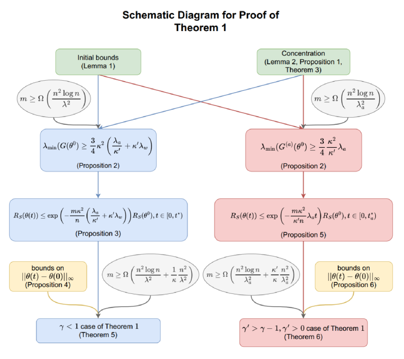
Figure 5: Sketch of proof for Theorem 1.

5.2 Condensed Regime

We remark that the $\{a_{k},\bm{w}_{k}\}_{k=1}^{m}$ dynamics

$$\frac{\mathrm{d}{a}_{k}}{\mathrm{d}{t}} =-\frac{\varepsilon}{\nu}\frac{1}{n}\sum_{i=1}^{n}e_{i}\frac{\sigma(\varepsilon{\bm{w}}_{k}^{\intercal}\bm{x}_{i})}{\varepsilon},$$ (5.13)

$$\frac{\mathrm{d}{\bm{w}}_{k}}{\mathrm{d}{t}} =-\frac{\nu}{\varepsilon}\frac{1}{n}\sum_{i=1}^{n}e_{i}{a}_{k}\sigma^{(1)}(\varepsilon{\bm{w}}_{k}^{\intercal}\bm{x}_{i})\bm{x}_{i},$$

is coupled in the sense that the solution of at least one of the equations in the system depends on knowing one of the other solutions in the system, and a coupled system is usually hard to solve.

However, in the condense regime, as $\varepsilon\ll 1$ and $\varepsilon\nu\ll\frac{1}{m}$, the evolution of $\{e_{i}\}_{i=1}^{n}$ is slow enough so that it remains close to $\{-y_{i}\}_{i=1}^{n}$ over a period of time $T>0$ at the initial stage, hence (5.13) approximately reads

$$\frac{\mathrm{d}a_{k}}{\mathrm{d}t} \approx\frac{\varepsilon}{\nu}\frac{1}{n}\sum_{i=1}^{n}y_{i}\bm{w}_{k}^{\intercal}\bm{x}_{i}=\frac{\varepsilon}{\nu}\bm{w}_{k}^{\intercal}\bm{z},$$ (5.14)

$$\frac{\mathrm{d}\bm{w}_{k}}{\mathrm{d}t} \approx\frac{\nu}{\varepsilon}\frac{1}{n}\sum_{i=1}^{n}y_{i}a_{k}\sigma^{(1)}(0)\bm{x}_{i}=\frac{\nu}{\varepsilon}a_{k}\bm{z},$$

and the coupled dynamics is reduced to linear dynamics.

We are able to solve out the linear dynamics (5.14) (Proposition 7), whose solutions read: For each $k\in[m]$, under the initial condition $\left[\nu a_{k}(0),\varepsilon\bm{w}_{k}^{\intercal}(0)\right]^{\intercal}=\left[\nu a_{k}^{0},(\varepsilon\bm{w}_{k}^{0})^{\intercal}\right]^{\intercal}$, we obtain that

$$\nu a_{k}(t) =\nu\left(\frac{1}{{2}}\exp(\lVert\bm{z}\rVert_{2}t)+\frac{1}{{2}}\exp(-\lVert\bm{z}\rVert_{2}t)\right)a_{k}^{0}$$ (5.15)

$$~{}~{}+{\varepsilon}\left(\frac{1}{{2}}\exp(\lVert\bm{z}\rVert_{2}t)-\frac{1}{{2}}\exp(-\lVert\bm{z}\rVert_{2}t)\right)\left<\bm{w}_{k}^{0},\hat{\bm{z}}\right>,$$

$$\varepsilon\bm{w}_{k}(t) ={\nu}\left(\frac{1}{{2}}\exp(\lVert\bm{z}\rVert_{2}t)-\frac{1}{{2}}\exp(-\lVert\bm{z}\rVert_{2}t)\right)a_{k}^{0}\hat{\bm{z}}$$

$$~{}~{}+{\varepsilon}\left(\frac{1}{{2}}\exp(\lVert\bm{z}\rVert_{2}t)+\frac{1}{{2}}\exp(-\lVert\bm{z}\rVert_{2}t)\right)\left<\bm{w}_{k}^{0},\hat{\bm{z}}\right>\hat{\bm{z}}$$

$$~{}~{}-{\varepsilon}\left<\bm{w}_{k}^{0},\hat{\bm{z}}\right>\hat{\bm{z}}+{\varepsilon}\bm{w}_{k}^{0}.$$

We remark that $\{a_{k},\bm{w}_{k}\}_{k=1}^{m}$ are the normalized parameters, then $\{\nu a_{k},\varepsilon\bm{w}_{k}\}_{k=1}^{m}$ corresponds to the original parameters in (3.4).

In the case where $\gamma>1$ and $0\leq\gamma^{\prime}<\gamma-1$ ($\bm{w}$-lag regime), as $\varepsilon\gg\nu$, then the magnitude of $\{\varepsilon\bm{w}_{k}\}_{k=1}^{m}$ is much larger than that of $\{\nu a_{k}\}_{k=1}^{m}$ at $t=0$. Based on (5.15), it can be observed that $\{\varepsilon\bm{w}_{k}\}_{k=1}^{m}$ remains dormant until $\{\nu a_{k}\}_{k=1}^{m}$ attain a magnitude that is commensurate with that of $\{\varepsilon\bm{w}_{k}\}_{k=1}^{m}$, and only then do the magnitudes of $\{\varepsilon\bm{w}_{k}\}_{k=1}^{m}$ and $\{\nu a_{k}\}_{k=1}^{m}$ experience exponential growth simultaneously. In order for the initial condensation of $\bm{\theta}_{\bm{w}}$ to be observed, one has to wait for some growth in the magnitude of $\{\varepsilon\bm{w}_{k}\}_{k=1}^{m}$, hence $T\sim\Omega(\log(m))$. More importantly, compared with the $\bm{w}$-lazy regime, the condition $\gamma^{\prime}<\gamma-1$ enforces $\varepsilon\ll\frac{1}{\sqrt{m}}$, thus providing enough room for $\{\varepsilon\bm{w}_{k}\}_{k=1}^{m}$ to grow in the $\bm{z}$-direction before $\{e_{i}\}_{i=1}^{n}$ deviates away from $\{-y_{i}\}_{i=1}^{m}$.

In the case where $\gamma>1$ and $\gamma^{\prime}<0$ ($a$-lag regime), as $\varepsilon\ll\nu$, then the initial magnitudes of $\{\varepsilon\bm{w}_{k}\}_{k=1}^{m}$ is much smaller than that of $\{\nu a_{k}\}_{k=1}^{m}$. Based on (5.15), it takes only $T\sim\Omega(1)$ for $\{\varepsilon\bm{w}_{k}\}_{k=1}^{m}$ to attain a magnitude comparable to $\{\nu a_{k}\}_{k=1}^{m}$, and this rapid growth leads to the observation of initial condensation towards the $\bm{z}$-direction, where $\gamma>1$ impose $\{e_{i}\}_{i=1}^{n}$ to a small neighbourhood of $\{-y_{i}\}_{i=1}^{m}$ for a period of time which is at least of order one. To end this part, we provide a sketch of the proofs for Theorem 2, see Figure 6.

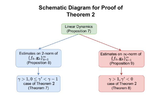
Figure 6: Sketch of proof for Theorem 2.

6 Conclusions

In this paper, we present the phase diagram of initial condensation for two-layer NNs with a wide class of smooth activation functions. We demonstrate the distinct features exhibited by NNs in the linear regime area and condensed regime area, and we provide a complete and detailed analysis for the transition across the boundary (critical regime) in the phase diagram. Moreover, in comparison with the work of Luo et al. [16], we identify the direction towards which the weight parameters condense, and we draw estimates on the time required for initial condensation to occur in contrast to the work of Zhou et al. [31]. The phase diagram at initial stage is crucial in that it is a valuable tool for understanding the implicit regularization effect provided by weight initialization schemes, and it serves as a cornerstone upon which future works can be done to provide thorough characterization of the dynamical behavior of general NNs at each of the identified regime.

In future, we endeavor to establish a framework for the analysis of initial condensation by a series of papers. In our upcoming publication, we plan to extend this formalism to Convolutional Neural Network (CNN) [20], and apply it to investigate the phenomenon of condensation for a wide range of NN architectures, including fully-connected deep network (DNN) and Residual Network (ResNet) [9].

Appendix A Several Estimates on the Initialization

We begin this part by an estimate on standard Gaussian vectors.

Lemma 1 (Bounds on initial parameters).

Given any $\delta\in(0,1)$, we have with probability at least $1-\delta$ over the choice of $\bm{\theta}^{0}$,

$$\max\limits_{k\in[m]}\left\{\lvert a_{k}^{0}\rvert,\;\lVert\bm{w}_{k}^{0}\rVert_{\infty}\right\}\leq\sqrt{2\log\frac{2m(d+1)}{\delta}},$$ (A.1)

Proof.

If $\textnormal{X}\sim\mathcal{N}(0,1)$, then for any $\eta>0$,

$$\mathbb{P}(\lvert\textnormal{X}\rvert>\eta)\leq 2\exp\left(-\frac{1}{2}\eta^{2}\right).$$

Since for $k\in[m]$,

$${a}_{k}^{0}\sim\mathcal{N}(0,1),\quad{\bm{w}}_{k}^{0}\sim\mathcal{N}(\bm{0},\bm{I}_{d}),$$

where

$${\bm{w}}_{k}^{0}:=\left[\left({w}_{k}^{0}\right)_{1},\left({w}_{k}^{0}\right)_{2},\cdots,\left({w}_{k}^{0}\right)_{d}\right]^{\intercal},$$

then for any $j\in[d]$,

$$\left({w}_{k}^{0}\right)_{j}\sim\mathcal{N}(0,1),$$

and they are all independent with each other. As we set

$$\eta=\sqrt{2\log\frac{2m(d+1)}{\delta}},$$

we obtain that

$$~{}~{}\mathbb{P}\left(\max\limits_{k\in[m]}\left\{\lvert a_{k}^{0}\rvert,\;\lVert\bm{w}_{k}^{0}\rVert_{\infty}\right\}>\eta\right)$$

$$=\mathbb{P}\left(\max\limits_{k\in[m],j\in[d]}\left\{\lvert a_{k}^{0}\rvert,\;\lvert{(w^{0}_{k})}_{j}\rvert\right\}>\eta\right)$$

$$=\mathbb{P}\left(\bigcup\limits_{k=1}^{m}\left[\left(\lvert a_{k}^{0}\rvert>\eta\right)\bigcup\left(\bigcup\limits_{j=1}^{d}\left(\lvert{(w_{k}^{0})}_{j}\rvert>\eta\right)\right)\right]\right)$$

$$\leq\sum_{k=1}^{m}\mathbb{P}\left(\lvert a_{k}^{0}\rvert>\eta\right)+\sum_{k=1}^{m}\sum_{j=1}^{d}\mathbb{P}\left(\lvert{(w^{0}_{k})}_{j}\rvert>\eta\right)$$

$$\leq 2m\exp\left(-\frac{1}{2}\eta^{2}\right)+2md\exp\left(-\frac{1}{2}\eta^{2}\right)$$

$$=2m(d+1)\exp\left({-\frac{1}{2}\eta^{2}}\right)=\delta.$$

∎

Next we would like to introduce the sub-exponential norm [25] of a random variable and Bernstein’s Inequality.

Definition 2 (Sub-exponential norm).

The sub-exponential norm of a random variable X is defined as

$$\lVert\textnormal{X}\rVert_{\psi_{1}}:=\inf\left\{s>0\mid\mathbb{E}_{\textnormal{X}}\left[\exp\left(\frac{\lvert\textnormal{X}\rvert}{s}\right)\right]\leq 2\right\}.$$ (A.2)

In particular, we denote $\textnormal{X}:=\chi^{2}(d)$ as a chi-square distribution with $d$ degrees of freedom [13], and its sub-exponential norm by

$$C_{\psi,d}:=\lVert\textnormal{X}\rVert_{\psi_{1}}.$$

Remark 7.

As the probability density function of $\textnormal{X}=\chi^{2}(d)$ reads

$$f_{\textnormal{X}}(z):=\frac{1}{2^{\frac{d}{2}}\Gamma(\frac{d}{2})}z^{\frac{d}{2}-1}\exp\left({-\frac{z}{2}}\right),\quad z\geq 0,$$

we note that

$$\mathbb{E}_{\textnormal{X}\sim\chi^{2}(1)}\exp\left(\frac{\lvert\textnormal{X}\rvert}{s}\right) =\int_{0}^{+\infty}\frac{1}{2^{\frac{1}{2}}\Gamma(\frac{1}{2})}z^{-\frac{1}{2}}\exp\left(-\left({\frac{1}{2}-\frac{1}{s}}\right)z\right)\mathop{}\!\mathrm{d}{z}=\frac{1}{\sqrt{1-\frac{2}{s}}},$$

Then we obtain that

$$\frac{8}{3}\leq C_{\psi,1}<3.$$

Moreover, we notice that

$$\mathbb{E}_{\textnormal{X}\sim\chi^{2}(d)}\exp\left(\frac{\lvert\textnormal{X}\rvert}{s}\right) =\left(\mathbb{E}_{\textnormal{Y}\sim\chi^{2}(1)}\exp\left(\frac{\lvert\textnormal{Y}\rvert}{s}\right)\right)^{d},$$

as we set

$$\frac{1}{\sqrt{1-\frac{2}{s}}}=2^{\frac{1}{d}},$$

then

$$s=\frac{2}{1-2^{-\frac{2}{d}}},$$

hence

$$\frac{2}{1-2^{-\frac{2}{d}}}\leq C_{\psi,d}<3,$$

and

$$C_{\psi,d}\geq C_{\psi,1},$$

for $d\geq 1$.

Lemma 2.

Given $\left\lVert\bm{x}\right\rVert_{2}\leq 1$ and $\left\lVert\bm{y}\right\rVert_{2}\leq 1$ equipped with $\sigma(\cdot):\mathbb{R}\to\mathbb{R}$, with $\sigma\in\mathcal{C}^{1}(\mathbb{R})$, satisfying

$$\sigma(0)=0,$$

and

$$\left\lVert\sigma^{(1)}(\cdot)\right\rVert_{\infty}\leq 1.$$

Under the condition that

$${a}\sim\mathcal{N}(0,1),\quad{\bm{w}}\sim\mathcal{N}(0,\bm{I}_{d}),$$

then for any $\varepsilon>0$,

• if

  $$\textnormal{X}_{1}:=\frac{1}{\varepsilon^{2}}\sigma(\varepsilon\bm{w}^{\intercal}\bm{x})\sigma(\varepsilon\bm{w}^{\intercal}\bm{y}),$$

  then

  $$\lVert\textnormal{X}_{1}\rVert_{\psi_{1}}\leq C_{\psi,d},$$

• and if

  $$\textnormal{X}_{2}:=a^{2}\sigma^{(1)}(\varepsilon\bm{w}^{\intercal}\bm{x})\sigma^{(1)}(\varepsilon\bm{w}^{\intercal}\bm{y})\left<\bm{x},\bm{y}\right>,$$

  then

  $$\lVert\textnormal{X}_{2}\rVert_{\psi_{1}}\leq C_{\psi,1}.$$

Proof.

Let

$$\textnormal{Z}:=\lVert\bm{w}\rVert^{2}_{2}\sim\chi^{2}(d).$$

Since

$$\left\lvert\textnormal{X}_{1}\right\rvert\leq\left\lvert\bm{w}^{\intercal}\bm{x}\right\rvert\left\lvert\bm{w}^{\intercal}\bm{y}\right\rvert=\lVert\bm{w}\rVert^{2}_{2},$$

then by definition,

$$\lVert\textnormal{X}_{1}\rVert_{\psi_{1}} =\inf\left\{s>0\mid\mathbb{E}_{\textnormal{X}_{1}}\exp\left(\frac{\left\lvert\textnormal{X}_{1}\right\rvert}{s}\right)\leq 2\right\}$$

$$=\inf\left\{s>0\mid\mathbb{E}_{\bm{w}}\exp\left(\frac{\left\lvert\sigma(\bm{w}^{\intercal}\bm{x})\sigma(\bm{w}^{\intercal}\bm{y})\right\rvert}{s}\right)\leq 2\right\}$$

$$\leq\inf\left\{s>0\mid\mathbb{E}_{\bm{w}}\exp\left(\frac{\lVert\bm{w}\rVert^{2}_{2}}{s}\right)\leq 2\right\},$$

hence

$$\lVert\textnormal{X}_{1}\rVert_{\psi_{1}}\leq C_{\psi,d}.$$ (A.3)

By similar reasoning, as

$$\left\lvert\textnormal{X}_{2}\right\rvert\leq a^{2},$$

hence

$$\lVert\textnormal{X}_{2}\rVert_{\psi_{1}}\leq C_{\psi,1}.$$ (A.4)

∎

We state an important theorem without proof, details of which can be found in [25].

Theorem 3 (Bernstein’s inequality).

Let $\{\textnormal{X}_{k}\}_{k=1}^{m}$ be i.i.d. sub-exponential random variables satisfying

$$\mathbb{E}\textnormal{X}_{1}=\mu,$$

then for any $\eta\geq 0$, we have

$$\mathbb{P}\left(\left\lvert\frac{1}{m}\sum_{k=1}^{m}\textnormal{X}_{k}-\mu\right\rvert\geq\eta\right)\leq 2\exp\left(-C_{0}m\min\left(\frac{\eta^{2}}{\lVert\textnormal{X}_{1}\rVert^{2}_{\psi_{1}}},\frac{\eta}{\lVert\textnormal{X}_{1}\rVert_{\psi_{1}}}\right)\right),$$

for some absolute constant $C_{0}$.

Proposition 1 (Upper and lower bounds of initial parameters).

Given any $\delta\in(0,1)$, if

$$m=\Omega\left(\log\frac{4}{\delta}\right),$$

then with probability at least $1-\delta$ over the choice of $\bm{\theta}^{0}$,

$$\sqrt{\frac{m}{2}} \leq\lVert\bm{\theta}_{a}^{0}\rVert_{2}\leq\sqrt{\frac{3m}{2}},$$ (A.5)

$$\sqrt{\frac{md}{2}} \leq\lVert\bm{\theta}_{\bm{w}}^{0}\rVert_{2}\leq\sqrt{\frac{3md}{2}},$$ (A.6)

and

$$\sqrt{\frac{m(d+1)}{2}}\leq\lVert\bm{\theta}^{0}\rVert_{2}\leq\sqrt{\frac{3m(d+1)}{2}}.$$ (A.7)

Proof.

Since

$$\left(a_{1}^{0}\right)^{2},\left(a_{2}^{0}\right)^{2},\cdots,\left(a_{m}^{0}\right)^{2}\sim\chi^{2}(1)$$

are i.i.d. sub-exponential random variables with

$$\mathbb{E}\left(a_{1}^{0}\right)^{2}=1.$$

By application of Theorem 3, we have

$$\mathbb{P}\left(\left\lvert\frac{1}{m}\sum_{k=1}^{m}\left(a_{k}^{0}\right)^{2}-1\right\rvert\geq\eta\right)\leq 2\exp\left(-C_{0}m\min\left(\frac{\eta^{2}}{C^{2}_{\psi,1}},\frac{\eta}{C_{\psi,1}}\right)\right),$$

since $C_{\psi,1}\geq\frac{8}{3}>2$, then for any $0\leq\eta\leq 2$, it is obvious that

$$\min\left(\frac{\eta^{2}}{C^{2}_{\psi,1}},\frac{\eta}{C_{\psi,1}}\right)=\frac{\eta^{2}}{C^{2}_{\psi,1}}.$$

We set

$$2\exp\left(-C_{0}m\frac{\eta^{2}}{C^{2}_{\psi,1}}\right)=\frac{\delta}{2},$$

and consequently,

$$\eta=\sqrt{\frac{C^{2}_{\psi,1}}{mC_{0}}\log\frac{4}{\delta}},$$

then with probability at least $1-\frac{\delta}{2}$ over the choice of $\bm{\theta}^{0}$,

$$m\left(1-\sqrt{\frac{C^{2}_{\psi,1}}{mC_{0}}\log\frac{4}{\delta}}\right)\leq\lVert\bm{\theta}_{a}^{0}\rVert^{2}_{2}\leq m\left(1+\sqrt{\frac{C^{2}_{\psi,1}}{mC_{0}}\log\frac{4}{\delta}}\right),$$ (A.8)

by choosing

$$m\geq{\frac{4C^{2}_{\psi,1}}{C_{0}}\log\frac{4}{\delta}},$$

we obtain that

$$\sqrt{\frac{m}{2}}\leq\lVert\bm{\theta}_{a}^{0}\rVert_{2}\leq\sqrt{\frac{3m}{2}}.$$

As for $\bm{\theta}_{\bm{w}}^{0}$, by application of Theorem 3,

$$\mathbb{P}\left(\left\lvert\frac{1}{md}\sum_{k=1}^{md}\left(w_{k}^{0}\right)^{2}-1\right\rvert\geq\eta\right)\leq 2\exp\left(-C_{0}md\min\left(\frac{\eta^{2}}{C^{2}_{\psi,1}},\frac{\eta}{C_{\psi,1}}\right)\right).$$

We set

$$2\exp\left(-C_{0}md\frac{\eta^{2}}{C^{2}_{\psi,1}}\right)=\frac{\delta}{2},$$

and consequently,

$$\eta=\sqrt{\frac{C^{2}_{\psi,1}}{mdC_{0}}\log\frac{4}{\delta}},$$

then with probability at least $1-\frac{\delta}{2}$ over the choice of $\bm{\theta}^{0}$,

$$md\left(1-\sqrt{\frac{C^{2}_{\psi,1}}{mdC_{0}}\log\frac{4}{\delta}}\right)\leq\lVert\bm{\theta}_{\bm{w}}^{0}\rVert^{2}_{2}\leq md\left(1+\sqrt{\frac{C^{2}_{\psi,1}}{mdC_{0}}\log\frac{4}{\delta}}\right),$$ (A.9)

by choosing

$$m\geq{\frac{4C^{2}_{\psi,1}}{dC_{0}}\log\frac{4}{\delta}},$$

we obtain that

$$\sqrt{\frac{md}{2}}\leq\lVert\bm{\theta}_{\bm{w}}^{0}\rVert_{2}\leq\sqrt{\frac{3md}{2}}.$$

Finally, as

$$\lVert\bm{\theta}^{0}\rVert_{2}^{2}=\lVert\bm{\theta}_{a}^{0}\rVert^{2}_{2}+\lVert\bm{\theta}_{\bm{w}}^{0}\rVert^{2}_{2},$$

then with probability at least $1-\delta$,

$$\sqrt{\frac{m(d+1)}{2}}\leq\lVert\bm{\theta}^{0}\rVert_{2}\leq\sqrt{\frac{3m(d+1)}{2}}.$$

∎

Appendix B Linear Regime

B.1 Full Rankness of the Gram matrices

We shall state two lemmas concerning full rankness of the Gram matrices, which have been stated as Lemma $\mathrm{F.1.}$ and Lemma $\mathrm{F.2.}$ in Du et al. [5].

Lemma 3.

Assume $\sigma(\cdot)$ is analytic and not a polynomial function. Consider input data set as $\mathcal{Z}=\{\bm{z}_{1},\bm{z}_{2},\dots,\bm{z}_{n}\}$, and non-parallel with each other, i.e., for any $j\neq k$,

$$\bm{z}_{j}\notin\mathrm{span}\left(\bm{z}_{k}\right),$$

we define

$$\bm{G}(\mathcal{Z}):=\left[\bm{G}(\mathcal{Z})_{ij}\right],$$ (B.1)

$$\bm{G}(\mathcal{Z})_{ij} :=\mathbb{E}_{\bm{w}\sim\mathcal{N}\left(\bm{0},\bm{I}\right)}\left[\sigma(\bm{w}^{\intercal}\bm{z}_{i})\sigma(\bm{w}^{\intercal}\bm{z}_{j})\right],$$

then $\lambda_{\min}\left(\bm{G}(\mathcal{Z})\right)>0.$

Similar to Lemma 3, we have another Lemma.

Lemma 4.

Assume $\sigma(\cdot)$ is analytic and not a polynomial function. Consider input data set as $\mathcal{Z}=\{\bm{z}_{1},\bm{z}_{2},\dots,\bm{z}_{n}\}$, and non-parallel with each other, we define

$$\bm{G}(\mathcal{Z}) :=\left[\bm{G}(\mathcal{Z})_{ij}\right],$$ (B.2)

$$\bm{G}(\mathcal{Z})_{ij} :=\mathbb{E}_{\bm{w}\sim\mathcal{N}\left(\bm{0},\bm{I}\right)}\left[\sigma^{(1)}(\bm{w}^{\intercal}\bm{z}_{i})\sigma^{(1)}(\bm{w}^{\intercal}\bm{z}_{j})\left<\bm{z}_{i},\bm{z}_{j}\right>\right],$$

then $\lambda_{\min}\left(\bm{G}(\mathcal{Z})\right)>0.$

We state an important theorem concerning the least eigenvalue of the normalized Gram matrices $\bm{K}^{[a]}$ and $\bm{K}^{[\bm{w}]}$ at infinite width limit. Recall that

$$K_{ij}^{[a]} =\frac{1}{\varepsilon^{2}}\mathbb{E}_{\bm{w}\sim\mathcal{N}\left(\bm{0},\bm{I}_{d}\right)}{\sigma(\varepsilon\bm{w}^{\intercal}\bm{x}_{i})\sigma(\varepsilon\bm{w}^{\intercal}\bm{x}_{j})},$$ (B.3)

$$K_{ij}^{[\bm{w}]} =\mathbb{E}_{(a,\bm{w})\sim\mathcal{N}\left(\bm{0},\bm{I}_{d+1}\right)}a^{2}\sigma^{(1)}(\varepsilon\bm{w}^{\intercal}\bm{x}_{i})\sigma^{(1)}(\varepsilon\bm{w}^{\intercal}\bm{x}_{j})\left<\bm{x}_{i},\bm{x}_{j}\right>.$$

Theorem 4 (Least eigenvalue of Gram matrices at infinite width).

Under 2 and 4, the normalized Gram matrices $\bm{K}^{[a]}$ and $\bm{K}^{[\bm{w}]}$ are strictly positive definite, and both of their least eigenvalues are of order $1$.

In other words, if we denote

$$\lambda:=\min\{\lambda_{a},\lambda_{\bm{w}}\}>0,$$

where

$$\lambda_{a}:=\lambda_{\min}\left(\bm{K}^{[a]}\right),\quad\lambda_{\bm{w}}:=\lambda_{\min}\left(\bm{K}^{[\bm{w}]}\right),$$ (B.4)

then

$$\lambda>0,$$

and

$$\lambda\sim\Omega(1).$$

Proof.

Since the following limit exists

$${\gamma}_{2}=\lim_{m\to\infty}-\frac{\log\varepsilon}{\log m},$$

then we conclude that

$$\lim_{m\to\infty}\varepsilon=0,$$

or

$$\lim_{m\to\infty}\varepsilon=1,$$

or

$$\lim_{m\to\infty}\varepsilon=+\infty,$$

and the normalized matrices $\bm{K}^{[a]}=\left[K_{ij}^{[a]}\right]_{n\times n}$ and $\bm{K}^{[\bm{w}]}=\left[K_{ij}^{[\bm{w}]}\right]_{n\times n}$ read

$$K_{ij}^{[a]} =\frac{1}{\varepsilon^{2}}\mathbb{E}_{\bm{w}\sim\mathcal{N}\left(\bm{0},\bm{I}_{d}\right)}{\sigma(\varepsilon\bm{w}^{\intercal}\bm{x}_{i})\sigma(\varepsilon\bm{w}^{\intercal}\bm{x}_{j})},$$

$$K_{ij}^{[\bm{w}]} =\mathbb{E}_{(a,\bm{w})\sim\mathcal{N}\left(\bm{0},\bm{I}_{d+1}\right)}a^{2}\sigma^{(1)}(\varepsilon\bm{w}^{\intercal}\bm{x}_{i})\sigma^{(1)}(\varepsilon\bm{w}^{\intercal}\bm{x}_{j})\left<\bm{x}_{i},\bm{x}_{j}\right>$$

$$=\mathbb{E}_{\bm{w}\sim\mathcal{N}\left(\bm{0},\bm{I}_{d}\right)}\sigma^{(1)}(\varepsilon\bm{w}^{\intercal}\bm{x}_{i})\sigma^{(1)}(\varepsilon\bm{w}^{\intercal}\bm{x}_{j})\left<\bm{x}_{i},\bm{x}_{j}\right>.$$

For the case where $\lim_{m\to\infty}\varepsilon=1$, by direct application of Lemma 3 and Lemma 4, $\lambda\sim\Omega(1)$ can be easily achieved.

For the case where $\lim_{m\to\infty}\varepsilon=0$, the normalized matrices read

$$K_{ij}^{[a]} =\lim_{m\to\infty}\frac{1}{\varepsilon^{2}}\mathbb{E}_{\bm{w}\sim\mathcal{N}\left(\bm{0},\bm{I}_{d}\right)}{\sigma(\varepsilon\bm{w}^{\intercal}\bm{x}_{i})\sigma(\varepsilon\bm{w}^{\intercal}\bm{x}_{j})}$$

$$=\mathbb{E}_{\bm{w}\sim\mathcal{N}\left(\bm{0},\bm{I}_{d}\right)}(\bm{w}^{\intercal}\bm{x}_{i})(\bm{w}^{\intercal}\bm{x}_{j}),$$

$$K_{ij}^{[\bm{w}]} =\lim_{m\to\infty}\mathbb{E}_{\bm{w}\sim\mathcal{N}\left(\bm{0},\bm{I}_{d}\right)}\sigma^{(1)}(\varepsilon\bm{w}^{\intercal}\bm{x}_{i})\sigma^{(1)}(\varepsilon\bm{w}^{\intercal}\bm{x}_{j})\left<\bm{x}_{i},\bm{x}_{j}\right>$$

$$=\mathbb{E}_{\bm{w}\sim\mathcal{N}\left(\bm{0},\bm{I}_{d}\right)}\left[\sigma^{(1)}(0)^{2}\right]\left<\bm{x}_{i},\bm{x}_{j}\right>$$

$$=\left<\bm{x}_{i},\bm{x}_{j}\right>.$$

hence both $\bm{K}^{[a]}$ and $\bm{K}^{[\bm{w}]}$ are independent of $\bm{\theta}_{\bm{w}}$ and $\bm{\theta}_{\bm{w}}$, and depend merely on the input sample $\mathcal{S}$. Consequently, $\lambda\sim\Omega(1)$.

For the case where $\lim_{m\to\infty}\varepsilon=+\infty$, the normalized matrices read

$$K_{ij}^{[a]} =\lim_{m\to\infty}\frac{1}{\varepsilon^{2}}\mathbb{E}_{\bm{w}\sim\mathcal{N}\left(\bm{0},\bm{I}_{d}\right)}{\sigma(\varepsilon\bm{w}^{\intercal}\bm{x}_{i})\sigma(\varepsilon\bm{w}^{\intercal}\bm{x}_{j})}$$

$$=\lim_{m\to\infty}\mathbb{E}_{\bm{w}\sim\mathcal{N}\left(\bm{0},\bm{I}_{d}\right)}\sigma^{(1)}(\varepsilon\bm{w}^{\intercal}\bm{x}_{i})\sigma^{(1)}(\varepsilon\bm{w}^{\intercal}\bm{x}_{j}),$$

$$K_{ij}^{[\bm{w}]} =\lim_{m\to\infty}\mathbb{E}_{\bm{w}\sim\mathcal{N}\left(\bm{0},\bm{I}_{d}\right)}\sigma^{(1)}(\varepsilon\bm{w}^{\intercal}\bm{x}_{i})\sigma^{(1)}(\varepsilon\bm{w}^{\intercal}\bm{x}_{j})\left<\bm{x}_{i},\bm{x}_{j}\right>,$$

where the entries of the matrix $\bm{K}^{[a]}$ exhibit leaky-ReLU-like behaviors. It has been proven in Du et al. [6] that under the unit data and nonparallel assumption, $\bm{K}^{[a]}$ is positive definite. Moreover, its expression can be explicitly computed, see [22]. As for the matrix $\bm{K}^{[\bm{w}]}$, we define a function $\bm{G}:\mathbb{R}^{n\times n}\to\mathbb{R}^{n\times n},$ such that

$$\bm{G}(\bm{K})_{ij}:={\bm{K}}_{ij}\mathbb{E}_{(u,v)^{\intercal}\sim\mathcal{N}\left(\bm{0},\begin{pmatrix}{\bm{K}}_{ii}&{\bm{K}}_{ij}\\ {\bm{K}}_{ji}&{\bm{K}}_{jj}\end{pmatrix}\right)}\sigma^{(1)}(u)\sigma^{(1)}(v).$$

We denote that $\bm{A}\succeq\bm{B}$ if and only if $\bm{A}-\bm{B}$ is a semi-positive definite matrix, and $\bm{A}\succ\bm{B}$ if and only if $\bm{A}-\bm{B}$ is a strictly positive definite matrix. Consequently, a scalar function $g(t)$ is defined as

$$g(t):=\min_{\bm{K}:\bm{K}\succ 0,~{}\frac{1}{c}\leq\bm{K}_{ii}\leq c,~{}\lambda_{\min}\left(\bm{K}\right)\geq t}\lambda_{\min}\left(\bm{G}(\bm{K})\right).$$

Then Lemma 4 guarantees that

$$g(\lambda_{0})>0,$$

and $\lambda\sim\Omega(1)$. ∎

Finally, we are hereby to show that the Gram matrix $\bm{G}$ at $t=0$ is also positive definite. Recall that

$$\bm{G}^{[a]}(\bm{\theta}) =\frac{\nu\varepsilon^{3}}{m}\sum_{k=1}^{m}\frac{1}{\varepsilon^{2}}\sigma(\varepsilon\bm{w}_{k}^{\intercal}\bm{x}_{i})\sigma(\varepsilon\bm{w}_{k}^{\intercal}\bm{x}_{j}),$$ (B.5)

$$\bm{G}^{[\bm{w}]}(\bm{\theta}) =\frac{\nu^{3}\varepsilon}{m}\sum_{k=1}^{m}a_{k}^{2}\sigma^{(1)}(\varepsilon\bm{w}_{k}^{\intercal}\bm{x}_{i})\sigma^{(1)}(\varepsilon\bm{w}_{k}^{\intercal}\bm{x}_{j})\left<\bm{x}_{i},\bm{x}_{j}\right>,$$

Proposition 2 (Least eigenvalue of initial Gram matrices).

Given any $\delta\in(0,1)$, under 2, 4 and 5, if

$$m=\Omega\left(\frac{n^{2}}{\lambda^{2}}\log\frac{4n^{2}}{\delta}\right),$$

where $\lambda=\min\{\lambda_{a},\lambda_{\bm{w}}\}$, whose definition can be found in Theorem 4. Then with probability at least $1-\delta$ over the choice of $\bm{\theta}^{0}$, we have

$$\lambda_{\min}\left(\bm{G}\left(\bm{\theta}^{0}\right)\right)\geq\frac{3}{4}\nu^{2}\varepsilon^{2}\left(\frac{\varepsilon}{\nu}\lambda_{a}+\frac{\nu}{\varepsilon}\lambda_{\bm{w}}\right).$$ (B.6)

Proof.

For any $\eta>0$ and all $i,j\in[n]$, we define the events

$$\Omega_{ij}^{[a]} :=\left\{\bm{\theta}^{0}\mid\left\lvert\frac{1}{\nu\varepsilon^{3}}G^{[a]}_{ij}\left(\bm{\theta}^{0}\right)-K^{[a]}_{ij}\right\rvert\leq\frac{\eta}{n}\right\},$$

$$\Omega_{ij}^{[\bm{w}]} :=\left\{\bm{\theta}^{0}\mid\left\lvert\frac{1}{\nu^{3}\varepsilon}G^{[\bm{w}]}_{ij}\left(\bm{\theta}^{0}\right)-K^{[\bm{w}]}_{ij}\right\rvert\leq\frac{\eta}{n}\right\}.$$

By application of Lemma 2 and Theorem 3, we obtain that for sufficiently small $\eta>0$, the following holds

$$\mathbb{P}(\Omega^{[a]}_{ij}) \geq 1-2\exp\left(-\frac{mC_{0}\eta^{2}}{n^{2}C_{\psi,d}^{2}}\right)$$

$$\mathbb{P}(\Omega^{[\bm{w}]}_{ij}) \geq 1-2\exp\left(-\frac{mC_{0}\eta^{2}}{n^{2}C_{\psi,1}^{2}}\right)\geq 1-2\exp\left(-\frac{mC_{0}\eta^{2}}{n^{2}C_{\psi,d}^{2}}\right),$$

hence with probability at least $1-4n^{2}\exp\left(-\frac{mC_{0}\eta^{2}}{n^{2}C_{\psi,d}^{2}}\right)$ over the choice of $\bm{\theta}^{0}$, we have

$$\left\lVert\frac{1}{\nu\varepsilon^{3}}\bm{G}^{[a]}\left(\bm{\theta}^{0}\right)-\bm{K}^{[a]}\right\rVert_{\mathrm{F}} \leq n\left\lVert\frac{1}{\nu\varepsilon^{3}}\bm{G}^{[a]}\left(\bm{\theta}^{0}\right)-\bm{K}^{[a]}\right\rVert_{\infty}\leq\eta,$$

$$\left\lVert\frac{1}{\nu^{3}\varepsilon}\bm{G}^{[\bm{w}]}\left(\bm{\theta}^{0}\right)-\bm{K}^{[\bm{w}]}\right\rVert_{\mathrm{F}} \leq n\left\lVert\frac{1}{\nu^{3}\varepsilon}\bm{G}^{[\bm{w}]}\left(\bm{\theta}^{0}\right)-\bm{K}^{[\bm{w}]}\right\rVert_{\infty}\leq\eta.$$

By taking $\eta=\frac{\lambda}{4}$,

$$\delta=4n^{2}\exp\left(-\frac{mC_{0}\lambda^{2}}{16n^{2}C_{\psi,d}^{2}}\right),$$

and we conclude that

$$\lambda_{\min}\left(\bm{G}\left(\bm{\theta}^{0}\right)\right) \geq\lambda_{\min}\left(\bm{G}^{[a]}\left(\bm{\theta}^{0}\right)\right)+\lambda_{\min}\left(\bm{G}^{[\bm{w}]}\left(\bm{\theta}^{0}\right)\right)$$

$$\geq{\nu\varepsilon^{3}}\lambda_{a}-{\nu\varepsilon^{3}}\left\lVert\frac{1}{\nu\varepsilon^{3}}\bm{G}^{[a]}\left(\bm{\theta}^{0}\right)-\bm{K}^{[a]}\right\rVert_{\mathrm{F}}$$

$$\quad+{\nu^{3}\varepsilon}\lambda_{\bm{w}}-{\nu^{3}\varepsilon}\left\lVert\frac{1}{\nu^{3}\varepsilon}\bm{G}^{[\bm{w}]}\left(\bm{\theta}^{0}\right)-\bm{K}^{[\bm{w}]}\right\rVert_{\mathrm{F}}$$

$$\geq{\nu\varepsilon^{3}}(\lambda_{a}-\eta)+{\nu^{3}\varepsilon}(\lambda_{\bm{w}}-\eta)$$

$$\geq\frac{3}{4}\nu^{2}\varepsilon^{2}\left(\frac{\varepsilon}{\nu}\lambda_{a}+\frac{\nu}{\varepsilon}\lambda_{\bm{w}}\right).$$

∎

B.2 $\bm{\theta}$-lazy Regime

In the rest of the paper, we define two quantities

$$\alpha(t):=\max\limits_{k\in[m],s\in[0,t]}\lvert a_{k}(s)\rvert,\quad\omega(t):=\max\limits_{k\in[m],s\in[0,t]}\lVert\bm{w}_{k}(s)\rVert_{\infty},$$ (B.7)

and we denote

$$t^{\ast}=\inf\{t\mid\bm{\theta}(t)\notin\mathcal{N}\left(\bm{\theta}^{0}\right)\},$$ (B.8)

where the event is defined as

$$\mathcal{N}\left(\bm{\theta}^{0}\right):=\left\{\bm{\theta}\mid\lVert\bm{G}(\bm{\theta})-\bm{G}\left(\bm{\theta}^{0}\right)\rVert_{\mathrm{F}}\leq\frac{1}{4}\nu^{2}\varepsilon^{2}\left(\frac{\varepsilon}{\nu}\lambda_{a}+\frac{\nu}{\varepsilon}\lambda_{\bm{w}}\right)\right\}.$$ (B.9)

We observe immediately that the event $\mathcal{N}\left(\bm{\theta}^{0}\right)\neq\varnothing$, since $\bm{\theta}^{0}\in\mathcal{N}\left(\bm{\theta}^{0}\right)$. Recall that $\lambda=\min\{\lambda_{a},\lambda_{\bm{w}}\}$, where

$$\lambda_{a}=\lambda_{\min}\left(\bm{K}^{[a]}\right),\quad\lambda_{\bm{w}}=\lambda_{\min}\left(\bm{K}^{[\bm{w}]}\right),$$

whose definition can be found in Theorem 4. Then we have the following lemma.

Proposition 3.

Given any $\delta\in(0,1)$, under 2, 4 and 5, if

$$m=\Omega\left(\frac{n^{2}}{\lambda^{2}}\log\frac{4n^{2}}{\delta}\right),$$

then with probability at least $1-\delta$ over the choice of $\bm{\theta}^{0}$, we have for any time $t\in[0,t^{\ast})$,

$$R_{S}(\bm{\theta}(t))\leq\exp\left(-\frac{m}{n}\nu^{2}\varepsilon^{2}\left(\frac{\varepsilon}{\nu}\lambda_{a}+\frac{\nu}{\varepsilon}\lambda_{\bm{w}}\right)t\right)R_{S}\left(\bm{\theta}^{0}\right).$$ (B.10)

Proof.

Proposition 2 implies that for any $\delta\in(0,1)$, with probability at least $1-\delta$ over the choice of $\bm{\theta}^{0}$ and for any $\bm{\theta}\in\mathcal{N}\left(\bm{\theta}^{0}\right)$, we have

$$\lambda_{\min}\left(\bm{G}(\bm{\theta})\right) \geq\lambda_{\min}\left(\bm{G}\left(\bm{\theta}^{0}\right)\right)-\lVert\bm{G}(\bm{\theta})-\bm{G}\left(\bm{\theta}^{0}\right)\rVert_{\mathrm{F}}$$

$$\geq\frac{3}{4}\nu^{2}\varepsilon^{2}\left(\frac{\varepsilon}{\nu}\lambda_{a}+\frac{\nu}{\varepsilon}\lambda_{\bm{w}}\right)-\frac{1}{4}\nu^{2}\varepsilon^{2}\left(\frac{\varepsilon}{\nu}\lambda_{a}+\frac{\nu}{\varepsilon}\lambda_{\bm{w}}\right)$$

$$=\frac{1}{2}\nu^{2}\varepsilon^{2}\left(\frac{\varepsilon}{\nu}\lambda_{a}+\frac{\nu}{\varepsilon}\lambda_{\bm{w}}\right).$$

Note that

$$G_{ij}(\bm{\theta}) =G_{ij}^{[a]}(\bm{\theta})+G^{[\bm{w}]}_{ij}(\bm{\theta})$$

$$=\frac{\nu\varepsilon^{3}}{m}\sum_{k=1}^{m}\frac{1}{\varepsilon^{2}}\sigma(\varepsilon\bm{w}_{k}^{\intercal}\bm{x}_{i})\sigma(\varepsilon\bm{w}_{k}^{\intercal}\bm{x}_{j})+\frac{\nu^{3}\varepsilon}{m}\sum_{k=1}^{m}a_{k}^{2}\sigma^{(1)}(\varepsilon\bm{w}_{k}^{\intercal}\bm{x}_{i})\sigma^{(1)}(\varepsilon\bm{w}_{k}^{\intercal}\bm{x}_{j})\left<\bm{x}_{i},\bm{x}_{j}\right>,$$

and the normalized flow

$$\nabla_{a_{k}}R_{S}(\bm{\theta}) ={\nu\varepsilon}\frac{1}{n}\sum_{i=1}^{n}e_{i}\frac{\sigma(\varepsilon{\bm{w}}_{k}^{\intercal}\bm{x}_{i})}{\varepsilon},$$

$$\nabla_{\bm{w}_{k}}R_{S}(\bm{\theta}) ={\nu\varepsilon}\frac{1}{n}\sum_{i=1}^{n}e_{i}{a}_{k}\sigma^{(1)}(\varepsilon{\bm{w}}_{k}^{\intercal}\bm{x}_{i})\bm{x}_{i}.$$

Finally, we obtain that

$$\frac{\mathrm{d}}{\mathrm{d}t}R_{S}(\bm{\theta}) =-\left(\sum_{k=1}^{m}\frac{\varepsilon}{\nu}\left<\nabla_{a_{k}}R_{S}(\bm{\theta}),\nabla_{a_{k}}R_{S}(\bm{\theta})\right>+\sum_{k=1}^{m}\frac{\nu}{\varepsilon}\left<\nabla_{\bm{w}_{k}}R_{S}(\bm{\theta}),\nabla_{\bm{w}_{k}}R_{S}(\bm{\theta})\right>\right)$$

$$=-\frac{m}{n^{2}}\bm{e}^{\intercal}\bm{G}(\bm{\theta})\bm{e}$$

$$\leq-\frac{2m}{n}\lambda_{\min}\left(\bm{G}(\bm{\theta})\right)R_{S}(\bm{\theta})$$

$$\leq-\frac{m}{n}\nu^{2}\varepsilon^{2}\left(\frac{\varepsilon}{\nu}\lambda_{a}+\frac{\nu}{\varepsilon}\lambda_{\bm{w}}\right)R_{S}(\bm{\theta}),$$

and immediate integration yields the result. ∎

Proposition 4.

Given any $\delta\in(0,1)$, under 2, 4 and 5, if $\gamma<1$, and

$$m=\max\left(\Omega\left(\frac{n^{2}}{\lambda^{2}}\log\frac{8n^{2}}{\delta}\right),\Omega\left(\left(\frac{n\sqrt{R_{S}\left(\bm{\theta}^{0}\right)}}{\lambda}\right)^{\frac{1}{1-\gamma}}\right)\right),$$

then with probability at least $1-\delta$ over the choice of $\bm{\theta}^{0}$, for any time $t\in[0,t^{\ast})$ and for any $k\in[m]$, both

$$\max\limits_{k\in[m]}\lvert a_{k}(t)-a_{k}(0)\rvert \leq 2\max\left\{\frac{\varepsilon}{\nu},1\right\}\sqrt{2\log\frac{4m(d+1)}{\delta}}p,$$ (B.11)

$$\max\limits_{k\in[m]}\lVert\bm{w}_{k}(t)-\bm{w}_{k}(0)\rVert_{\infty} \leq 2\max\left\{\frac{\nu}{\varepsilon},1\right\}\sqrt{2\log\frac{4m(d+1)}{\delta}}p,$$

and

$$\max\limits_{k\in[m]}\{\lvert a_{k}(0)\rvert,\;\lVert\bm{w}_{k}(0)\rVert_{\infty}\}\leq\sqrt{2\log\frac{4m(d+1)}{\delta}},$$ (B.12)

hold, where

$$p:=\frac{2\sqrt{2}dn\sqrt{R_{S}\left(\bm{\theta}^{0}\right)}}{m\nu\varepsilon\left(\frac{\varepsilon}{\nu}\lambda_{a}+\frac{\nu}{\varepsilon}\lambda_{\bm{w}}\right)}.$$

Proof.

Since

$$\alpha(t)=\max\limits_{k\in[m],s\in[0,t]}\left\lvert a_{k}(s)\right\rvert,\quad\omega(t)=\max\limits_{k\in[m],s\in[0,t]}\left\lVert\bm{w}_{k}(s)\right\rVert_{\infty},$$

we obtain

$$\left\lvert\nabla_{a_{k}}R_{S}\right\rvert^{2} =\left\lvert\frac{1}{n}\sum_{i=1}^{n}e_{i}\nu\sigma(\varepsilon\bm{w}_{k}^{\intercal}\bm{x}_{i})\right\rvert^{2}\leq 2\lVert\varepsilon\bm{w}_{k}\rVert^{2}_{1}\nu^{2}R_{S}(\bm{\theta})\leq 2d^{2}(\omega(t))^{2}\nu^{2}\varepsilon^{2}R_{S}(\bm{\theta}),$$

$$\lVert\nabla_{\bm{w}_{k}}R_{S}\rVert^{2} =\left\lVert\frac{1}{n}\sum_{i=1}^{n}e_{i}\nu\varepsilon a_{k}\sigma^{(1)}(\varepsilon\bm{w}_{k}^{\intercal}\bm{x}_{i})\bm{x}_{i}\right\rVert^{2}_{\infty}\leq 2\lvert a_{k}\rvert^{2}\nu^{2}\varepsilon^{2}R_{S}(\bm{\theta})\leq 2(\alpha(t))^{2}\nu^{2}\varepsilon^{2}R_{S}(\bm{\theta}).$$

By Proposition 2 and Proposition 3, we have if

$$m\geq\frac{16n^{2}C_{\psi,d}^{2}}{\lambda^{2}C_{0}}\log\frac{8n^{2}}{\delta},$$

then with probability at least $1-\frac{\delta}{2}$ over the choice of $\bm{\theta}^{0}$, we have that

$$\left\lvert a_{k}(t)-a_{k}(0)\right\rvert \leq\frac{\varepsilon}{\nu}\int_{0}^{t}\lvert\nabla_{a_{k}}R_{S}(\bm{\theta}(s))\rvert\mathop{}\!\mathrm{d}{s}$$

$$\leq{\sqrt{2}d\varepsilon^{2}}\int_{0}^{t}\omega(s)\sqrt{R_{S}(\bm{\theta}(s))}\mathop{}\!\mathrm{d}{s}$$

$$\leq{\sqrt{2}d\varepsilon^{2}}\omega(t)\int_{0}^{t}\sqrt{R_{S}\left(\bm{\theta}^{0}\right)}\exp\left(-\frac{m}{2n}\nu^{2}\varepsilon^{2}\left(\frac{\varepsilon}{\nu}\lambda_{a}+\frac{\nu}{\varepsilon}\lambda_{\bm{w}}\right)t\right)\mathop{}\!\mathrm{d}{s}$$

$$\leq{\sqrt{2}d\varepsilon^{2}}\omega(t)\int_{0}^{\infty}\sqrt{R_{S}\left(\bm{\theta}^{0}\right)}\exp\left(-\frac{m}{2n}\nu^{2}\varepsilon^{2}\left(\frac{\varepsilon}{\nu}\lambda_{a}+\frac{\nu}{\varepsilon}\lambda_{\bm{w}}\right)t\right)\mathop{}\!\mathrm{d}{s}$$

$$=\frac{2\sqrt{2}dn\sqrt{R_{S}\left(\bm{\theta}^{0}\right)}}{m\nu^{2}\left(\frac{\varepsilon}{\nu}\lambda_{a}+\frac{\nu}{\varepsilon}\lambda_{\bm{w}}\right)}\omega(t)=\frac{\varepsilon}{\nu}{p}\omega(t),$$

and

$$\left\lVert\bm{w}_{k}(t)-\bm{w}_{k}(0)\right\rVert_{\infty} \leq\frac{\nu}{\varepsilon}\int_{0}^{t}\left\lVert\nabla_{\bm{w}_{k}}R_{S}(\bm{\theta}(s))\right\rVert_{\infty}\mathop{}\!\mathrm{d}{s}$$

$$\leq\sqrt{2}\nu^{2}\int_{0}^{t}\alpha(s)\sqrt{R_{S}(\bm{\theta}(s))}\mathop{}\!\mathrm{d}{s}$$

$$\leq\sqrt{2}\nu^{2}\alpha(t)\int_{0}^{t}\sqrt{R_{S}\left(\bm{\theta}^{0}\right)}\exp\left(-\frac{m}{2n}\nu^{2}\varepsilon^{2}\left(\frac{\varepsilon}{\nu}\lambda_{a}+\frac{\nu}{\varepsilon}\lambda_{\bm{w}}\right)t\right)\mathop{}\!\mathrm{d}{s}$$

$$\leq\sqrt{2}\nu^{2}\alpha(t)\int_{0}^{\infty}\sqrt{R_{S}\left(\bm{\theta}^{0}\right)}\exp\left(-\frac{m}{2n}\nu^{2}\varepsilon^{2}\left(\frac{\varepsilon}{\nu}\lambda_{a}+\frac{\nu}{\varepsilon}\lambda_{\bm{w}}\right)t\right)\mathop{}\!\mathrm{d}{s}$$

$$=\frac{2\sqrt{2}n\sqrt{R_{S}\left(\bm{\theta}^{0}\right)}}{m\varepsilon^{2}\left(\frac{\varepsilon}{\nu}\lambda_{a}+\frac{\nu}{\varepsilon}\lambda_{\bm{w}}\right)}\alpha(t)\leq\frac{2\sqrt{2}dn\sqrt{R_{S}\left(\bm{\theta}^{0}\right)}}{m\varepsilon^{2}\left(\frac{\varepsilon}{\nu}\lambda_{a}+\frac{\nu}{\varepsilon}\lambda_{\bm{w}}\right)}\alpha(t)=\frac{\nu}{\varepsilon}p\alpha(t).$$

Thus

$$\alpha(t) \leq\alpha(0)+\frac{\varepsilon}{\nu}{p}\omega(t),$$

$$\omega(t) \leq\omega(0)+\frac{\nu}{\varepsilon}p\alpha(t),$$

moreover, by Lemma 1, we have with probability at least $1-\frac{\delta}{2}$ over the choice of $\bm{\theta}^{0}$, as

$$\max\limits_{k\in[m]}\{\lvert a_{k}(0)\rvert,\;\lVert\bm{w}_{k}(0)\rVert_{\infty}\}\leq\sqrt{2\log\frac{4m(d+1)}{\delta}},$$

then

$$\alpha(0)\leq\sqrt{2\log\frac{4m(d+1)}{\delta}},\quad\omega(0)\leq\sqrt{2\log\frac{4m(d+1)}{\delta}}$$

Hence if

$$m\geq\left(\frac{2\sqrt{2}dn\sqrt{R_{S}\left(\bm{\theta}^{0}\right)}}{\lambda}\right)^{\frac{1}{1-\gamma}},$$

we have

$$p=\frac{2\sqrt{2}dn\sqrt{R_{S}\left(\bm{\theta}^{0}\right)}}{m\nu\varepsilon\left(\frac{\varepsilon}{\nu}\lambda_{a}+\frac{\nu}{\varepsilon}\lambda_{\bm{w}}\right)}\leq\frac{\sqrt{2}dn\sqrt{R_{S}\left(\bm{\theta}^{0}\right)}}{m\nu\varepsilon\lambda}\leq\frac{1}{2}.$$

Thus

$$\alpha(t)\leq\alpha(0)+\frac{\varepsilon}{\nu}p\omega(0)+p^{2}\alpha(t),$$

hence

$$\alpha(t)\leq\frac{4}{3}\alpha(0)+\frac{2}{3}\frac{\varepsilon}{\nu}\omega(0).$$

Therefore

$$\alpha(t)\leq 2\max\left\{\frac{\varepsilon}{\nu},1\right\}\sqrt{2\log\frac{4m(d+1)}{\delta}}.$$

Similarly, one can obtain the estimate of $\omega(t)$ as

$$\omega(t)\leq 2\max\left\{\frac{\nu}{\varepsilon},1\right\}\sqrt{2\log\frac{4m(d+1)}{\delta}}.$$

To sum up, for any $t\in[0,t^{\ast})$, with probability at least $1-\delta$ over the choice of $\bm{\theta}^{0}$,

$$\max\limits_{k\in[m]}\left\lvert a_{k}(t)-a_{k}(0)\right\rvert \leq 2\max\left\{\frac{\varepsilon}{\nu},1\right\}\sqrt{2\log\frac{4m(d+1)}{\delta}}p,$$

$$\max\limits_{k\in[m]}\left\lVert\bm{w}_{k}(t)-\bm{w}_{k}(0)\right\rVert_{\infty} \leq 2\max\left\{\frac{\nu}{\varepsilon},1\right\}\sqrt{2\log\frac{4m(d+1)}{\delta}}p.$$

∎

Theorem 5.

Given any $\delta\in(0,1)$, under 2, 4 and 5, if $\gamma<1$ and

$$m=\max\Bigg{(} \Omega\left(\frac{n^{2}}{\lambda^{2}}\log\frac{16n^{2}}{\delta}\right),\Omega\left(\left(\frac{n\sqrt{R_{S}\left(\bm{\theta}^{0}\right)}}{\lambda}\right)^{\frac{1}{1-\gamma}}\right),$$ (B.13)

$$\Omega\left(\left(\frac{n^{2}\sqrt{R_{S}\left(\bm{\theta}^{0}\right)}}{\lambda^{2}}\right)^{\frac{1}{1-\gamma}}\right),\Omega\left(\log\frac{8}{\delta}\right)\Bigg{)},$$

then with probability at least $1-\frac{\delta}{2}$ over the choice of $\bm{\theta}^{0}$, we have for all time $t>0$,

$$R_{S}(\bm{\theta}(t))\leq\exp\left(-\frac{2m\nu^{2}\varepsilon^{2}\lambda t}{n}\right)R_{S}\left(\bm{\theta}^{0}\right),$$ (B.14)

and with probability at least $1-\delta$ over the choice of $\bm{\theta}^{0}$,

$$\lim_{m\to\infty}\sup\limits_{t\in[0,+\infty)}\frac{\lVert\bm{\theta}_{\bm{w}}(t)-\bm{\theta}_{\bm{w}}(0)\rVert_{2}}{\lVert\bm{\theta}_{\bm{w}}(0)\rVert_{2}}=0.$$ (B.15)

Remark 8.

In this scenario, we also obtain that with probability at least $1-\delta$ over the choice of $\bm{\theta}^{0}$,

$$\lim_{m\to\infty}\sup\limits_{t\in[0,+\infty)}\frac{\lVert\bm{\theta}(t)-\bm{\theta}(0)\rVert_{2}}{\lVert\bm{\theta}(0)\rVert_{2}}=0.$$ (B.16)

Proof.

According to Proposition 4, it suffices to show that $t^{\ast}=\infty$.

(i). Firstly, from Proposition 3, we have with probability at least $1-\frac{\delta}{2}$ over the choice of $\bm{\theta}^{0}$, for any $t\in[0,t^{\ast})$, the following holds

$$\left\lvert a_{k}(t)-a_{k}(0)\right\rvert \leq\frac{\varepsilon}{\nu}p\omega(t)\leq 2\max\left\{\frac{\varepsilon}{\nu},1\right\}\xi p,$$

$$\left\lVert\bm{w}_{k}(t)-\bm{w}_{k}(0)\right\rVert_{\infty} \leq\frac{\nu}{\varepsilon}p\alpha(t)\leq 2\max\left\{\frac{\nu}{\varepsilon},1\right\}\xi p,$$

where

$$p=\frac{2\sqrt{2}dn\sqrt{R_{S}\left(\bm{\theta}^{0}\right)}}{m\nu\varepsilon\left(\frac{\varepsilon}{\nu}\lambda_{a}+\frac{\nu}{\varepsilon}\lambda_{\bm{w}}\right)},$$

and

$$\xi:=\sqrt{2\log\frac{8m(d+1)}{\delta}}.$$

For $m$ large enough, i.e.,

$$m\geq\left(\frac{2\sqrt{2}dn\sqrt{R_{S}\left(\bm{\theta}^{0}\right)}}{\lambda}\right)^{\frac{1}{1-\gamma}},$$

then we have

$$p=\frac{2\sqrt{2}dn\sqrt{R_{S}\left(\bm{\theta}^{0}\right)}}{m\nu\varepsilon\left(\frac{\varepsilon}{\nu}\lambda_{a}+\frac{\nu}{\varepsilon}\lambda_{\bm{w}}\right)}\leq\frac{\sqrt{2}dn\sqrt{R_{S}\left(\bm{\theta}^{0}\right)}}{m\nu\varepsilon\lambda}\leq\frac{1}{2}.$$

It is noteworthy to emphasize that the demonstration of (B.14) requires solely the utilization of the aforementioned relations.

(ii). Let

$$g^{[a]}_{ij}(\bm{w}):=\frac{1}{\varepsilon^{2}}\sigma(\varepsilon\bm{w}^{\intercal}\bm{x}_{i})\sigma(\varepsilon\bm{w}^{\intercal}\bm{x}_{j}),$$

then

$$\left\lvert G_{ij}^{[a]}(\bm{\theta}(t))-G_{ij}^{[a]}(\bm{\theta}(0))\right\rvert\leq\frac{\nu\varepsilon^{3}}{m}\sum_{k=1}^{m}\left\lvert g^{[a]}_{ij}(\bm{w}_{k}(t))-g^{[a]}_{ij}(\bm{w}_{k}(0))\right\rvert.$$

By mean value theorem, for some $c\in(0,1)$,

$$\left\lvert g^{[a]}_{ij}(\bm{w}_{k}(t))-g^{[a]}_{ij}(\bm{w}_{k}(0))\right\rvert\leq\left\lVert\nabla_{\bm{w}}g^{[a]}_{ij}\left(c\bm{w}_{k}(t)+(1-c)\bm{w}_{k}(0)\right)\right\rVert_{\infty}\lVert\bm{w}_{k}(t)-\bm{w}_{k}(0)\rVert_{1},$$

where

$$\nabla_{\bm{w}}g_{ij}^{[a]}(\bm{w})=\frac{1}{\varepsilon}\sigma^{(1)}(\varepsilon\bm{w}^{\intercal}\bm{x}_{i})\sigma(\varepsilon\bm{w}^{\intercal}\bm{x}_{j})\bm{x}_{i}+\frac{1}{\varepsilon}\sigma(\varepsilon\bm{w}^{\intercal}\bm{x}_{i})\sigma^{(1)}(\varepsilon\bm{w}^{\intercal}\bm{x}_{j})\bm{x}_{j},$$

and

$$\left\lVert\nabla_{\bm{w}}g_{ij}^{[a]}(\bm{w})\right\rVert_{\infty}\leq 2\lVert\bm{w}\rVert_{1}.$$

then

$$\left\lVert\bm{w}_{k}(t)-\bm{w}_{k}(0)\right\rVert_{1}\leq 2d\max\left\{\frac{\nu}{\varepsilon},1\right\}\xi p,$$

thus, we have

$$\left\lVert c\bm{w}_{k}(t)+(1-c)\bm{w}_{k}(0)\right\rVert_{1} \leq d\left(\lVert\bm{w}_{k}(0)\rVert_{\infty}+\lVert\bm{w}_{k}(t)-\bm{w}_{k}(0)\rVert_{\infty}\right)$$

$$\leq d\left(\xi+2\max\left\{\frac{\nu}{\varepsilon},1\right\}\xi p\right)$$

$$\leq d\left(\xi+\max\left\{\frac{\nu}{\varepsilon},1\right\}\xi\right)$$

$$\leq 2\max\left\{\frac{\nu}{\varepsilon},1\right\}d\xi,$$

hence

$$\left\lvert G_{ij}^{[a]}(\bm{\theta}(t))-G_{ij}^{[a]}(\bm{\theta}(0))\right\rvert \leq\frac{\nu\varepsilon^{3}}{m}\sum_{k=1}^{m}\left\lvert g^{[a]}_{ij}(\bm{w}_{k}(t))-g^{[a]}_{ij}(\bm{w}_{k}(0))\right\rvert$$

$$\leq 8d^{2}{\nu^{2}\varepsilon^{2}}\xi^{2}\max\left\{\frac{\nu}{\varepsilon},\frac{\varepsilon}{\nu}\right\}p,$$

then by using the same technique in Proposition 2,

$$\left\lVert\bm{G}^{[a]}(\bm{\theta}(t))-\bm{G}^{[a]}(\bm{\theta}(0))\right\rVert_{\mathrm{F}}$$

$$~{}~{}\leq 8d^{2}n{\nu^{2}\varepsilon^{2}}\max\left\{\frac{\nu}{\varepsilon},\frac{\varepsilon}{\nu}\right\}\left(2\log\frac{8m(d+1)}{\delta}\right)\frac{2\sqrt{2}dn\sqrt{R_{S}\left(\bm{\theta}^{0}\right)}}{m\nu\varepsilon\left(\frac{\varepsilon}{\nu}\lambda_{a}+\frac{\nu}{\varepsilon}\lambda_{\bm{w}}\right)}$$

$$\leq\nu\varepsilon\max\left\{\frac{\nu}{\varepsilon},\frac{\varepsilon}{\nu}\right\}\frac{32\sqrt{2}d^{3}n^{2}\left(\log\frac{8m(d+1)}{\delta}\right)\sqrt{R_{S}\left(\bm{\theta}^{0}\right)}}{m\left(\frac{\varepsilon}{\nu}\lambda_{a}+\frac{\nu}{\varepsilon}\lambda_{\bm{w}}\right)}.$$

We shall notice that as

$$\frac{1}{\lambda^{2}} \geq 16\left(\frac{1}{27}\right)^{\frac{1}{2}}\frac{1}{\left(\left(\frac{\varepsilon}{\nu}\right)^{\frac{3}{2}}\lambda_{a}+\left(\frac{\nu}{\varepsilon}\right)^{\frac{1}{2}}\lambda_{\bm{w}}\right)^{2}}$$

$$=16\left(\frac{1}{27}\right)^{\frac{1}{2}}\frac{\nu}{\varepsilon}\frac{1}{\left(\frac{\varepsilon}{\nu}\lambda_{a}+\frac{\nu}{\varepsilon}\lambda_{\bm{w}}\right)^{2}},$$

and

$$\frac{1}{\lambda^{2}} \geq 16\left(\frac{1}{27}\right)^{\frac{1}{2}}\frac{1}{\left(\left(\frac{\varepsilon}{\nu}\right)^{\frac{1}{2}}\lambda_{a}+\left(\frac{\nu}{\varepsilon}\right)^{\frac{3}{2}}\lambda_{\bm{w}}\right)^{2}}$$

$$=16\left(\frac{1}{27}\right)^{\frac{1}{2}}\frac{\varepsilon}{\nu}\frac{1}{\left(\frac{\varepsilon}{\nu}\lambda_{a}+\frac{\nu}{\varepsilon}\lambda_{\bm{w}}\right)^{2}}.$$

As $\gamma<1$, then we may choose $m$ large enough, such that

$$m\nu\varepsilon \geq\frac{96\sqrt{2}d^{3}n^{2}\left(\log\frac{8m(d+1)}{\delta}\right)\sqrt{R_{S}\left(\bm{\theta}^{0}\right)}}{\lambda^{2}}$$

$$\geq\frac{256\sqrt{2}d^{3}n^{2}\left(\log\frac{8m(d+1)}{\delta}\right)\sqrt{R_{S}\left(\bm{\theta}^{0}\right)}}{16\left(\frac{1}{27}\right)^{\frac{1}{2}}\lambda^{2}}$$

$$\geq\max\left\{\frac{\nu}{\varepsilon},\frac{\varepsilon}{\nu}\right\}\frac{256\sqrt{2}d^{3}n^{2}\left(\log\frac{8m(d+1)}{\delta}\right)\sqrt{R_{S}\left(\bm{\theta}^{0}\right)}}{\left(\frac{\varepsilon}{\nu}\lambda_{a}+\frac{\nu}{\varepsilon}\lambda_{\bm{w}}\right)^{2}}.$$

Then for any $t\in[0,t^{\ast})$,

$$\left\lVert\bm{G}^{[a]}(\bm{\theta}(t))-\bm{G}^{[a]}(\bm{\theta}(0))\right\rVert_{\mathrm{F}}\leq\frac{1}{8}\nu^{2}\varepsilon^{2}\left(\frac{\varepsilon}{\nu}\lambda_{a}+\frac{\nu}{\varepsilon}\lambda_{\bm{w}}\right).$$ (B.17)

(iii). As for $\bm{G}^{[\bm{w}]}(\bm{\theta}(t))$, we observe that directly from Proposition 3, for any $t\in[0,t^{\ast})$, the following holds

$$\left\lvert G^{[\bm{w}]}_{ij}(\bm{\theta}(t))-G^{[\bm{w}]}_{ij}(\bm{\theta}(0))\right\rvert$$

$$\leq\frac{\nu^{3}\varepsilon\left\lvert\left<\bm{x}_{i},\bm{x}_{j}\right>\right\rvert}{m}\Bigg{(}\sum_{k=1}^{m}\Big{|}a_{k}^{2}(t)\sigma^{(1)}\left(\left<\bm{w}_{k}(t),\bm{x}_{i}\right>\right)\sigma^{(1)}\left(\left<\bm{w}_{k}(t),\bm{x}_{j}\right>\right)$$

$$~{}~{}~{}~{}~{}~{}~{}~{}~{}~{}~{}~{}~{}~{}~{}~{}~{}~{}~{}~{}~{}~{}~{}~{}~{}~{}~{}~{}~{}~{}-a_{k}^{2}(0)\sigma^{(1)}\left(\left<\bm{w}_{k}(0),\bm{x}_{i}\right>\right)\sigma^{(1)}\left(\left<\bm{w}_{k}(0),\bm{x}_{j}\right>\right)\Big{|}\Bigg{)},$$

we define a new quantity

$$D_{k,i,j}(t):=\sigma^{(1)}\left(\left<\bm{w}_{k}(t),\bm{x}_{i}\right>\right)\sigma^{(1)}\left(\left<\bm{w}_{k}(t),\bm{x}_{j}\right>\right)-\sigma^{(1)}\left(\left<\bm{w}_{k}(0),\bm{x}_{i}\right>\right)\sigma^{(1)}\left(\left<\bm{w}_{k}(0),\bm{x}_{j}\right>\right),$$

then we obtain that

$$\left\lvert G^{[\bm{w}]}_{ij}(\bm{\theta}(t))-G^{[\bm{w}]}_{ij}(\bm{\theta}(0))\right\rvert$$

$$\leq\frac{\nu^{3}\varepsilon}{m}\sum_{k=1}^{m}\left(a_{k}^{2}(t)D_{k,i,j}(t)+\left\lvert a_{k}^{2}(t)-a_{k}^{2}(0)\right\rvert\right).$$

We shall make an estimate on the quantity $D_{k,i,j}(t)$:

$$D_{k,i,j}(t) =\sigma^{(1)}\left(\left<\bm{w}_{k}(t),\bm{x}_{i}\right>\right)\sigma^{(1)}\left(\left<\bm{w}_{k}(t),\bm{x}_{j}\right>\right)-\sigma^{(1)}\left(\left<\bm{w}_{k}(t),\bm{x}_{i}\right>\right)\sigma^{(1)}\left(\left<\bm{w}_{k}(0),\bm{x}_{j}\right>\right)$$

$$~{}~{}+\sigma^{(1)}\left(\left<\bm{w}_{k}(t),\bm{x}_{i}\right>\right)\sigma^{(1)}\left(\left<\bm{w}_{k}(0),\bm{x}_{j}\right>\right)-\sigma^{(1)}\left(\left<\bm{w}_{k}(0),\bm{x}_{i}\right>\right)\sigma^{(1)}\left(\left<\bm{w}_{k}(0),\bm{x}_{j}\right>\right)$$

$$\leq\left\lvert\left<\bm{w}_{k}(t),\bm{x}_{i}\right>-\left<\bm{w}_{k}(0),\bm{x}_{i}\right>\right\rvert+\left\lvert\left<\bm{w}_{k}(t),\bm{x}_{j}\right>-\left<\bm{w}_{k}(0),\bm{x}_{j}\right>\right\rvert$$

$$\leq 2\left\lVert\bm{w}_{k}(t)-\bm{w}_{k}(0)\right\rVert_{1}\leq 2d\left\lVert\bm{w}_{k}(t)-\bm{w}_{k}(0)\right\rVert_{\infty}$$

$$\leq 4d\max\left\{\frac{\nu}{\varepsilon},1\right\}\xi p.$$

Hence, we observe that

$$\left\lvert a_{k}^{2}(t)-a_{k}^{2}(0)\right\rvert \leq\left\lvert a_{k}(t)-a_{k}(0)\right\rvert^{2}+2\left\lvert a_{k}(0)\right\rvert\left\lvert a_{k}(t)-a_{k}(0)\right\rvert$$

$$\leq\left(2\max\left\{\frac{\varepsilon}{\nu},1\right\}\xi p\right)^{2}+2\xi\left(2\max\left\{\frac{\varepsilon}{\nu},1\right\}\xi p\right)$$

$$\leq 6\max\left\{\left(\frac{\varepsilon}{\nu}\right)^{2},1\right\}\xi^{2}p,$$

and consequently

$$a_{k}(t)^{2} \leq\left\lvert a_{k}^{2}(t)-a_{k}^{2}(0)\right\rvert+a_{k}^{2}(0)$$

$$\leq 6\xi^{2}\max\left\{\left(\frac{\varepsilon}{\nu}\right)^{2},1\right\}p+\xi^{2}$$

$$\leq 3\xi^{2}\max\left\{\left(\frac{\varepsilon}{\nu}\right)^{2},1\right\}+\xi^{2}$$

$$\leq 4\max\left\{\left(\frac{\varepsilon}{\nu}\right)^{2},1\right\}\xi^{2}.$$

Thus, we have

$$\left\lvert G^{[\bm{w}]}_{ij}(\bm{\theta}(t))-G^{[\bm{w}]}_{ij}(\bm{\theta}(0))\right\rvert$$

$$\leq\frac{\nu^{3}\varepsilon}{m}\sum_{k=1}^{m}\left(a_{k}^{2}(t)D_{k,i,j}(t)+\left\lvert a_{k}^{2}(t)-a_{k}^{2}(0)\right\rvert\right)$$

$$\leq\nu^{3}\varepsilon\left(16d\max\left\{\left(\frac{\varepsilon}{\nu}\right)^{2},\frac{\nu}{\varepsilon}\right\}\xi^{3}p+6\max\left\{\left(\frac{\varepsilon}{\nu}\right)^{2},1\right\}\xi^{2}p\right)$$

$$\leq\nu^{3}\varepsilon\left(16d\max\left\{\left(\frac{\varepsilon}{\nu}\right)^{2},\frac{\nu}{\varepsilon}\right\}\xi^{3}p+6d\max\left\{\left(\frac{\varepsilon}{\nu}\right)^{2},1\right\}\xi^{2}p\right)$$

$$\leq 24\nu^{2}\varepsilon^{2}d\left(2\log\frac{8m(d+1)}{\delta}\right)^{\frac{3}{2}}\max\left\{\left(\frac{\nu}{\varepsilon}\right)^{2},\frac{\varepsilon}{\nu}\right\}p,$$

then by using the same technique in Proposition 2,

$$\left\lVert G^{[\bm{w}]}(\bm{\theta}(t))-G^{[\bm{w}]}(\bm{\theta}(0))\right\rVert_{\mathrm{F}}$$

$$\leq n\left\lVert G^{[\bm{w}]}_{ij}(\bm{\theta}(t))-G^{[\bm{w}]}_{ij}(\bm{\theta}(0))\right\rVert_{\infty}$$

$$\leq 24\nu^{2}\varepsilon^{2}d\left(2\log\frac{8m(d+1)}{\delta}\right)^{\frac{3}{2}}\max\left\{\left(\frac{\nu}{\varepsilon}\right)^{2},\frac{\varepsilon}{\nu}\right\}np$$

$$=\nu\varepsilon\max\left\{\left(\frac{\nu}{\varepsilon}\right)^{2},\frac{\varepsilon}{\nu}\right\}\frac{96d^{2}n^{2}\left(\log\frac{8m(d+1)}{\delta}\right)^{\frac{3}{2}}\sqrt{R_{S}\left(\bm{\theta}^{0}\right)}}{m\left(\frac{\varepsilon}{\nu}\lambda_{a}+\frac{\nu}{\varepsilon}\lambda_{\bm{w}}\right)},$$

We notice that as

$$\frac{1}{\lambda^{2}} \geq\frac{\left(\frac{\nu}{\varepsilon}\right)^{2}}{\left(\frac{\nu}{\varepsilon}\lambda_{\bm{w}}\right)^{2}}=\left(\frac{\nu}{\varepsilon}\right)^{2}\frac{1}{\left(\frac{\varepsilon}{\nu}\lambda_{a}+\frac{\nu}{\varepsilon}\lambda_{\bm{w}}\right)^{2}},$$

and

$$\frac{1}{\lambda^{2}} \geq 16\left(\frac{1}{27}\right)^{\frac{1}{2}}\frac{1}{\left(\left(\frac{\varepsilon}{\nu}\right)^{\frac{1}{2}}\lambda_{a}+\left(\frac{\nu}{\varepsilon}\right)^{\frac{3}{2}}\lambda_{\bm{w}}\right)^{2}}$$

$$=16\left(\frac{1}{27}\right)^{\frac{1}{2}}\frac{\varepsilon}{\nu}\frac{1}{\left(\frac{\varepsilon}{\nu}\lambda_{a}+\frac{\nu}{\varepsilon}\lambda_{\bm{w}}\right)^{2}}.$$

As $\gamma<1$, then we may choose $m$ large enough, such that

$$m\nu\varepsilon \geq\frac{384d^{2}n^{2}\left(\log\frac{8m(d+1)}{\delta}\right)^{\frac{3}{2}}\sqrt{R_{S}\left(\bm{\theta}^{0}\right)}}{\lambda^{2}}$$

$$\geq\max\left\{\frac{384d^{2}n^{2}\left(\log\frac{8m(d+1)}{\delta}\right)^{\frac{3}{2}}\sqrt{R_{S}\left(\bm{\theta}^{0}\right)}}{\lambda^{2}},\frac{384d^{2}n^{2}\left(\log\frac{8m(d+1)}{\delta}\right)^{\frac{3}{2}}\sqrt{R_{S}\left(\bm{\theta}^{0}\right)}}{16\left(\frac{1}{27}\right)^{\frac{1}{2}}\lambda^{2}}\right\}$$

$$\geq\max\left\{\left(\frac{\nu}{\varepsilon}\right)^{2},\frac{\varepsilon}{\nu}\right\}\frac{d^{2}n^{2}\left(\log\frac{8m(d+1)}{\delta}\right)^{\frac{3}{2}}\sqrt{R_{S}\left(\bm{\theta}^{0}\right)}}{\left(\frac{\varepsilon}{\nu}\lambda_{a}+\frac{\nu}{\varepsilon}\lambda_{\bm{w}}\right)^{2}}.$$

Then for any $t\in[0,t^{\ast})$,

$$\left\lVert\bm{G}^{[\bm{w}]}(\bm{\theta}(t))-\bm{G}^{[\bm{w}]}(\bm{\theta}(0))\right\rVert_{\mathrm{F}}\leq\frac{1}{8}\nu^{2}\varepsilon^{2}\left(\frac{\varepsilon}{\nu}\lambda_{a}+\frac{\nu}{\varepsilon}\lambda_{\bm{w}}\right).$$ (B.18)

To sum up, for $t\in[0,t^{\ast})$, the following holds

$$R_{S}(\bm{\theta}(t))\leq\exp\left(-\frac{m}{n}\nu^{2}\varepsilon^{2}\left(\frac{\varepsilon}{\nu}\lambda_{a}+\frac{\nu}{\varepsilon}\lambda_{\bm{w}}\right)t\right)R_{S}\left(\bm{\theta}^{0}\right).$$

Suppose we have $t^{\ast}<+\infty$, then one can take the limit $t\to t^{\ast}$ in (B.17) and (B.18), which leads to a contradiction with the definition of $t^{\ast}$. Therefore $t^{\ast}=+\infty$.

Directly from Proposition 1, we have with probability at least $1-\frac{\delta}{2}$ over the choice of $\bm{\theta}^{0}$,

$$\left\lVert\bm{\theta}_{\bm{w}}^{0}\right\rVert_{2}\geq\sqrt{\frac{md}{2}},$$

thus we have

$$\sup\limits_{t\in[0,+\infty)}\frac{\lVert\bm{\theta}_{\bm{w}}(t)-\bm{\theta}_{\bm{w}}(0)\rVert_{2}}{\lVert\bm{\theta}_{\bm{w}}(0)\rVert_{2}} \leq\sqrt{\frac{2}{md}}\sup\limits_{t\in[0,+\infty)}\left\lVert\bm{\theta}_{\bm{w}}(t)-\bm{\theta}_{\bm{w}}(0)\right\rVert_{2},$$

via Proposition 4, with probability at least $1-\frac{\delta}{2}$ over the choice of $\bm{\theta}^{0}$,

$$\max\limits_{k\in[m]}\left\lVert\bm{w}_{k}(t)-\bm{w}_{k}(0)\right\rVert_{\infty} \leq 2\max\left\{\frac{\nu}{\varepsilon},1\right\}\xi p,$$

then

$$\left\lVert\bm{\theta}_{\bm{w}}(t)-\bm{\theta}_{\bm{w}}(0)\right\rVert_{2} \leq\left[\sum_{k=1}^{m}\left(\left\lVert\bm{w}_{k}(t)-\bm{w}_{k}(0)\right\rVert_{\infty}^{2}\right)\right]^{\frac{1}{2}}$$

$$\leq 2\max\left\{\frac{\nu}{\varepsilon},1\right\}\sqrt{md}\xi p$$

$$\leq 2\max\left\{\frac{\nu}{\varepsilon},1\right\}\sqrt{md}\sqrt{2\log\frac{8m(d+1)}{\delta}}\frac{2\sqrt{2}dn\sqrt{R_{S}\left(\bm{\theta}^{0}\right)}}{m\nu\varepsilon\left(\frac{\varepsilon}{\nu}\lambda_{a}+\frac{\nu}{\varepsilon}\lambda_{\bm{w}}\right)}$$

$$\leq 8\max\left\{\frac{\nu}{\varepsilon},1\right\}\sqrt{\log\frac{8m(d+1)}{\delta}}\frac{d^{\frac{3}{2}}n\sqrt{R_{S}\left(\bm{\theta}^{0}\right)}}{\sqrt{m}\nu\varepsilon\left(\frac{\varepsilon}{\nu}\lambda_{a}+\frac{\nu}{\varepsilon}\lambda_{\bm{w}}\right)},$$

hence

$$\sup\limits_{t\in[0,+\infty)}\frac{\lVert\bm{\theta}_{\bm{w}}(t)-\bm{\theta}_{\bm{w}}(0)\rVert_{2}}{\lVert\bm{\theta}_{\bm{w}}(0)\rVert_{2}} \leq\sqrt{\frac{2}{md}}\sup\limits_{t\in[0,+\infty)}\left\lVert\bm{\theta}_{\bm{w}}(t)-\bm{\theta}_{\bm{w}}(0)\right\rVert_{2}$$

$$\leq 8\sqrt{2}\max\left\{\frac{\nu}{\varepsilon},1\right\}\sqrt{\log\frac{8m(d+1)}{\delta}}\frac{dn\sqrt{R_{S}\left(\bm{\theta}^{0}\right)}}{{m}\nu\varepsilon\left(\frac{\varepsilon}{\nu}\lambda_{a}+\frac{\nu}{\varepsilon}\lambda_{\bm{w}}\right)}$$

$$\leq 4\sqrt{2}\sqrt{\log\frac{8m(d+1)}{\delta}}\frac{dn\sqrt{R_{S}\left(\bm{\theta}^{0}\right)}}{{m}\nu\varepsilon\lambda},$$

as $\gamma<1$, then we obtain that

$$\sup\limits_{t\in[0,+\infty)}\frac{\lVert\bm{\theta}_{\bm{w}}(t)-\bm{\theta}_{\bm{w}}(0)\rVert_{2}}{\lVert\bm{\theta}_{\bm{w}}(0)\rVert_{2}}\lesssim\frac{\sqrt{\log\frac{8m(d+1)}{\delta}}}{m^{1-\gamma}},$$ (B.19)

hence

$$\lim_{m\to\infty}\sup\limits_{t\in[0,+\infty)}\frac{\lVert\bm{\theta}_{\bm{w}}(t)-\bm{\theta}_{\bm{w}}(0)\rVert_{2}}{\lVert\bm{\theta}_{\bm{w}}(0)\rVert_{2}}=0.$$ (B.20)

Similarly, directly from Proposition 1, we have with probability at least $1-\frac{\delta}{2}$ over the choice of $\bm{\theta}^{0}$,

$$\left\lVert\bm{\theta}^{0}\right\rVert_{2}\geq\sqrt{\frac{m(d+1)}{2}},$$

thus we have

$$\sup\limits_{t\in[0,+\infty)}\frac{\lVert\bm{\theta}(t)-\bm{\theta}(0)\rVert_{2}}{\lVert\bm{\theta}(0)\rVert_{2}} \leq\sqrt{\frac{2}{m(d+1)}}\sup\limits_{t\in[0,+\infty)}\left\lVert\bm{\theta}(t)-\bm{\theta}(0)\right\rVert_{2},$$

via Proposition 4, with probability at least $1-\frac{\delta}{2}$ over the choice of $\bm{\theta}^{0}$,

$$\max\limits_{k\in[m]}\left\lvert a_{k}(t)-a_{k}(0)\right\rvert \leq 2\max\left\{\frac{\varepsilon}{\nu},1\right\}\xi p,$$

$$\max\limits_{k\in[m]}\left\lVert\bm{w}_{k}(t)-\bm{w}_{k}(0)\right\rVert_{\infty} \leq 2\max\left\{\frac{\nu}{\varepsilon},1\right\}\xi p,$$

then

$$\left\lVert\bm{\theta}(t)-\bm{\theta}(0)\right\rVert_{2} \leq\left[\sum_{k=1}^{m}\left(\left\lvert a_{k}(t)-a_{k}(0)\right\rvert^{2}+\left\lVert\bm{w}_{k}(t)-\bm{w}_{k}(0)\right\rVert_{\infty}^{2}\right)\right]^{\frac{1}{2}}$$

$$\leq 2\max\left\{\frac{\varepsilon}{\nu},\frac{\nu}{\varepsilon}\right\}\sqrt{m(d+1)}\xi p$$

$$\leq 2\max\left\{\frac{\varepsilon}{\nu},\frac{\nu}{\varepsilon}\right\}\sqrt{m(d+1)}\sqrt{2\log\frac{8m(d+1)}{\delta}}\frac{2\sqrt{2}dn\sqrt{R_{S}\left(\bm{\theta}^{0}\right)}}{m\nu\varepsilon\left(\frac{\varepsilon}{\nu}\lambda_{a}+\frac{\nu}{\varepsilon}\lambda_{\bm{w}}\right)}$$

$$\leq 8\max\left\{\frac{\varepsilon}{\nu},\frac{\nu}{\varepsilon}\right\}\sqrt{\log\frac{8m(d+1)}{\delta}}\frac{\sqrt{d+1}dn\sqrt{R_{S}\left(\bm{\theta}^{0}\right)}}{\sqrt{m}\nu\varepsilon\left(\frac{\varepsilon}{\nu}\lambda_{a}+\frac{\nu}{\varepsilon}\lambda_{\bm{w}}\right)},$$

hence

$$\sup\limits_{t\in[0,+\infty)}\frac{\lVert\bm{\theta}(t)-\bm{\theta}(0)\rVert_{2}}{\lVert\bm{\theta}(0)\rVert_{2}} \leq\sqrt{\frac{2}{m(d+1)}}\sup\limits_{t\in[0,+\infty)}\left\lVert\bm{\theta}(t)-\bm{\theta}(0)\right\rVert_{2}$$

$$\leq 8\sqrt{2}\max\left\{\frac{\varepsilon}{\nu},\frac{\nu}{\varepsilon}\right\}\sqrt{\log\frac{8m(d+1)}{\delta}}\frac{dn\sqrt{R_{S}\left(\bm{\theta}^{0}\right)}}{{m}\nu\varepsilon\left(\frac{\varepsilon}{\nu}\lambda_{a}+\frac{\nu}{\varepsilon}\lambda_{\bm{w}}\right)}$$

$$\leq 8\sqrt{2}\sqrt{\log\frac{8m(d+1)}{\delta}}\frac{dn\sqrt{R_{S}\left(\bm{\theta}^{0}\right)}}{{m}\nu\varepsilon\lambda},$$

as $\gamma<1$, then we obtain that

$$\sup\limits_{t\in[0,+\infty)}\frac{\lVert\bm{\theta}(t)-\bm{\theta}(0)\rVert_{2}}{\lVert\bm{\theta}(0)\rVert_{2}}\lesssim\frac{\sqrt{\log\frac{8m(d+1)}{\delta}}}{m^{1-\gamma}},$$ (B.21)

moreover,

$$\lim_{m\to\infty}\sup\limits_{t\in[0,+\infty)}\frac{\lVert\bm{\theta}(t)-\bm{\theta}(0)\rVert_{2}}{\lVert\bm{\theta}(0)\rVert_{2}}=0.$$ (B.22)

∎

B.3 $\bm{w}$-lazy Regime

We denote

$$t_{a}^{\ast}=\inf\{t\mid\bm{\theta}(t)\notin\mathcal{N}\left(\bm{\theta}^{0}\right)\},$$ (B.23)

where the event is defined as

$$\mathcal{N}_{a}\left(\bm{\theta}^{0}\right):=\left\{\bm{\theta}\mid\lVert\bm{G}^{[a]}(\bm{\theta})-\bm{G}^{[a]}\left(\bm{\theta}^{0}\right)\rVert_{\mathrm{F}}\leq\frac{1}{4}\nu\varepsilon^{3}\lambda_{a}\right\}.$$ (B.24)

We observe immediately that the event $\mathcal{N}_{a}\left(\bm{\theta}^{0}\right)\neq\varnothing$, since $\bm{\theta}^{0}\in\mathcal{N}_{a}\left(\bm{\theta}^{0}\right)$. Recall that

$$\lambda_{a}=\lambda_{\min}\left(\bm{K}^{[a]}\right),$$

whose definition can be found in Theorem 4.

Proposition 5.

Given any $\delta\in(0,1)$, under 2, 4 and 5, if

$$m=\Omega\left(\frac{n^{2}}{\lambda_{a}^{2}}\log\frac{4n^{2}}{\delta}\right),$$

then with probability at least $1-\delta$ over the choice of $\bm{\theta}^{0}$, we have for any time $t\in[0,t_{a}^{\ast})$,

$$R_{S}(\bm{\theta}(t))\leq\exp\left(-\frac{m}{n}\nu\varepsilon^{3}\lambda_{a}t\right)R_{S}\left(\bm{\theta}^{0}\right).$$ (B.25)

Proof.

Similar to the proof in Proposition 3, with probability at least $1-\delta$ over the choice of $\bm{\theta}^{0}$ and for any $\bm{\theta}\in\mathcal{N}\left(\bm{\theta}^{0}\right)$, we have

$$\lambda_{\min}\left(\bm{G}(\bm{\theta})\right) \geq\lambda_{\min}\left(\bm{G}^{[a]}(\bm{\theta})\right)$$

$$\geq\lambda_{\min}\left(\bm{G}^{[a]}\left(\bm{\theta}^{0}\right)\right)-\lVert\bm{G}^{[a]}(\bm{\theta})-\bm{G}^{[a]}\left(\bm{\theta}^{0}\right)\rVert_{\mathrm{F}}$$

$$\geq\frac{1}{2}\nu^{3}\varepsilon\lambda_{a}.$$

Finally, we obtain that

$$\frac{\mathrm{d}}{\mathrm{d}t}R_{S}(\bm{\theta}(t)) =-\frac{m}{n^{2}}\bm{e}^{\intercal}\bm{G}(\bm{\theta}(t))\bm{e}$$

$$\leq-\frac{2m}{n}\lambda_{\min}\left(\bm{G}(\bm{\theta}(t))\right)R_{S}(\bm{\theta}(t))$$

$$\leq-\frac{m}{n}\nu^{3}\varepsilon\lambda_{a}R_{S}(\bm{\theta}(t)),$$

and immediate integration yields the result. ∎

Proposition 6.

Given any $\delta\in(0,1)$, under 2, 4 and 5, if $\gamma>1$, $\gamma^{\prime}>\gamma-1$, and

$$m=\max\left(\Omega\left(\frac{n^{2}}{\lambda_{a}^{2}}\log\frac{8n^{2}}{\delta}\right),\Omega\left(\frac{n\sqrt{R_{S}\left(\bm{\theta}^{0}\right)}}{\lambda_{a}}\right)^{\frac{1}{1-\gamma+\gamma^{\prime}}}\right),$$

then with probability at least $1-\delta$ over the choice of $\bm{\theta}^{0}$, for any time $t\in[0,t_{a}^{\ast})$ and for any $k\in[m]$, both

$$\max\limits_{k\in[m]}\lvert a_{k}(t)-a_{k}(0)\rvert \leq 2\frac{\varepsilon}{\nu}\sqrt{2\log\frac{4m(d+1)}{\delta}}p_{a},$$ (B.26)

$$\max\limits_{k\in[m]}\lVert\bm{w}_{k}(t)-\bm{w}_{k}(0)\rVert_{\infty} \leq 2\sqrt{2\log\frac{4m(d+1)}{\delta}}p_{a},$$

and

$$\max\limits_{k\in[m]}\{\lvert a_{k}(0)\rvert,\;\lVert\bm{w}_{k}(0)\rVert_{\infty}\}\leq\sqrt{2\log\frac{4m(d+1)}{\delta}},$$ (B.27)

hold, where

$$p_{a}:=\frac{2\sqrt{2}dn\sqrt{R_{S}\left(\bm{\theta}^{0}\right)}}{m\varepsilon^{2}\lambda_{a}}.$$

Proof.

Since

$$\alpha(t)=\max\limits_{k\in[m],s\in[0,t]}\left\lvert a_{k}(s)\right\rvert,\quad\omega(t)=\max\limits_{k\in[m],s\in[0,t]}\left\lVert\bm{w}_{k}(s)\right\rVert_{\infty},$$

we obtain

$$\left\lvert\nabla_{a_{k}}R_{S}\right\rvert^{2} =\left\lvert\frac{1}{n}\sum_{i=1}^{n}e_{i}\nu\sigma(\varepsilon\bm{w}_{k}^{\intercal}\bm{x}_{i})\right\rvert^{2}\leq 2\lVert\varepsilon\bm{w}_{k}\rVert^{2}_{1}\nu^{2}R_{S}(\bm{\theta})\leq 2d^{2}(\omega(t))^{2}\nu^{2}\varepsilon^{2}R_{S}(\bm{\theta}),$$

$$\lVert\nabla_{\bm{w}_{k}}R_{S}\rVert^{2} =\left\lVert\frac{1}{n}\sum_{i=1}^{n}e_{i}\nu\varepsilon a_{k}\sigma^{(1)}(\varepsilon\bm{w}_{k}^{\intercal}\bm{x}_{i})\bm{x}_{i}\right\rVert^{2}_{\infty}\leq 2\lvert a_{k}\rvert^{2}\nu^{2}\varepsilon^{2}R_{S}(\bm{\theta})\leq 2(\alpha(t))^{2}\nu^{2}\varepsilon^{2}R_{S}(\bm{\theta}).$$

By Proposition 5, we have if

$$m\geq\frac{16n^{2}d^{2}C_{\psi,d}^{2}}{\lambda^{2}C_{0}}\log\frac{8n^{2}}{\delta},$$

then with probability at least $1-\frac{\delta}{2}$ over the choice of $\bm{\theta}^{0}$, we have that

$$\left\lvert a_{k}(t)-a_{k}(0)\right\rvert \leq\frac{\varepsilon}{\nu}\int_{0}^{t}\lvert\nabla_{a_{k}}R_{S}(\bm{\theta}(s))\rvert\mathop{}\!\mathrm{d}{s}$$

$$\leq{\sqrt{2}d\varepsilon^{2}}\int_{0}^{t}\omega(s)\sqrt{R_{S}(\bm{\theta}(s))}\mathop{}\!\mathrm{d}{s}$$

$$\leq{\sqrt{2}d\varepsilon^{2}}\omega(t)\int_{0}^{t}\sqrt{R_{S}\left(\bm{\theta}^{0}\right)}\exp\left(-\frac{m}{2n}\nu^{2}\varepsilon^{2}\left(\frac{\varepsilon}{\nu}\lambda_{a}+\frac{\nu}{\varepsilon}\lambda_{\bm{w}}\right)t\right)\mathop{}\!\mathrm{d}{s}$$

$$\leq{\sqrt{2}d\varepsilon^{2}}\omega(t)\int_{0}^{\infty}\sqrt{R_{S}\left(\bm{\theta}^{0}\right)}\exp\left(-\frac{m}{2n}\nu^{2}\varepsilon^{2}\left(\frac{\varepsilon}{\nu}\lambda_{a}+\frac{\nu}{\varepsilon}\lambda_{\bm{w}}\right)t\right)\mathop{}\!\mathrm{d}{s}$$

$$=\frac{2\sqrt{2}dn\sqrt{R_{S}\left(\bm{\theta}^{0}\right)}}{m\nu^{2}\left(\frac{\varepsilon}{\nu}\lambda_{a}+\frac{\nu}{\varepsilon}\lambda_{\bm{w}}\right)}\omega(t)$$

$$\leq\frac{2\sqrt{2}dn\sqrt{R_{S}\left(\bm{\theta}^{0}\right)}}{m\nu\varepsilon\lambda_{a}}\omega(t)$$

$$\leq\frac{\varepsilon}{\nu}p_{a}\omega(t),$$

and similarly

$$\left\lVert\bm{w}_{k}(t)-\bm{w}_{k}(0)\right\rVert_{\infty} \leq\frac{\nu}{\varepsilon}\int_{0}^{t}\left\lVert\nabla_{\bm{w}_{k}}R_{S}(\bm{\theta}(s))\right\rVert_{\infty}\mathop{}\!\mathrm{d}{s}$$

$$\leq\sqrt{2}\nu^{2}\int_{0}^{t}\alpha(s)\sqrt{R_{S}(\bm{\theta}(s))}\mathop{}\!\mathrm{d}{s}$$

$$\leq\sqrt{2}\nu^{2}\alpha(t)\int_{0}^{t}\sqrt{R_{S}\left(\bm{\theta}^{0}\right)}\exp\left(-\frac{m}{2n}\nu^{2}\varepsilon^{2}\left(\frac{\varepsilon}{\nu}\lambda_{a}+\frac{\nu}{\varepsilon}\lambda_{\bm{w}}\right)t\right)\mathop{}\!\mathrm{d}{s}$$

$$\leq\sqrt{2}\nu^{2}\alpha(t)\int_{0}^{\infty}\sqrt{R_{S}\left(\bm{\theta}^{0}\right)}\exp\left(-\frac{m}{2n}\nu^{2}\varepsilon^{2}\left(\frac{\varepsilon}{\nu}\lambda_{a}+\frac{\nu}{\varepsilon}\lambda_{\bm{w}}\right)t\right)\mathop{}\!\mathrm{d}{s}$$

$$=\frac{2\sqrt{2}n\sqrt{R_{S}\left(\bm{\theta}^{0}\right)}}{m\varepsilon^{2}\left(\frac{\varepsilon}{\nu}\lambda_{a}+\frac{\nu}{\varepsilon}\lambda_{\bm{w}}\right)}\alpha(t)$$

$$\leq\frac{2\sqrt{2}dn\sqrt{R_{S}\left(\bm{\theta}^{0}\right)}}{m\frac{\varepsilon^{3}}{\nu}\lambda_{a}}\alpha(t)$$

$$\leq\frac{\nu}{\varepsilon}p_{a}\alpha(t).$$

Thus

$$\alpha(t) \leq\alpha(0)+\frac{\varepsilon}{\nu}p_{a}\omega(t),$$

$$\omega(t) \leq\omega(0)+\frac{\nu}{\varepsilon}p_{a}\alpha(t),$$

moreover, by Lemma 1, with probability at least $1-\frac{\delta}{2}$ over the choice of $\bm{\theta}^{0}$,

$$\max\limits_{k\in[m]}\{\lvert a_{k}(0)\rvert,\;\lVert\bm{w}_{k}(0)\rVert_{\infty}\}\leq\sqrt{2\log\frac{4m(d+1)}{\delta}}.$$

Then, if

$$m\geq\left(\frac{4\sqrt{2}dn\sqrt{R_{S}\left(\bm{\theta}^{0}\right)}}{\lambda_{a}}\right)^{\frac{1}{1-\gamma+\gamma^{\prime}}},$$

we have

$$p_{a}=\frac{2\sqrt{2}dn\sqrt{R_{S}\left(\bm{\theta}^{0}\right)}}{m\varepsilon^{2}\lambda_{a}}\leq\frac{1}{2}.$$

Therefore

$$\alpha(t)\leq 2\max\left\{\frac{\varepsilon}{\nu},1\right\}\sqrt{2\log\frac{4m(d+1)}{\delta}}=2\frac{\varepsilon}{\nu}\sqrt{2\log\frac{4m(d+1)}{\delta}}.$$

Similarly, one can obtain the estimate of $\omega(t)$ as

$$\omega(t)\leq 2\max\left\{\frac{\nu}{\varepsilon},1\right\}\sqrt{2\log\frac{4m(d+1)}{\delta}}=2\sqrt{2\log\frac{4m(d+1)}{\delta}}.$$

Hence, for any $t\in[0,t_{a}^{\ast})$, with probability at least $1-\delta$ over the choice of $\bm{\theta}^{0}$,

$$\max\limits_{k\in[m]}\left\lvert a_{k}(t)-a_{k}(0)\right\rvert \leq 2\frac{\varepsilon}{\nu}\sqrt{2\log\frac{4m(d+1)}{\delta}}p_{a},$$

$$\max\limits_{k\in[m]}\left\lVert\bm{w}_{k}(t)-\bm{w}_{k}(0)\right\rVert_{\infty} \leq 2\sqrt{2\log\frac{4m(d+1)}{\delta}}p_{a}.$$

∎

Theorem 6.

Given any $\delta\in(0,1)$, under 2, 4 and 5, if $\gamma\geq 1$, $\gamma^{\prime}>\gamma-1$, and

$$m=\max\Bigg{(} \Omega\left(\frac{n^{2}}{\lambda_{a}^{2}}\log\frac{16n^{2}}{\delta}\right),\Omega\left(\left(\frac{n\sqrt{R_{S}\left(\bm{\theta}^{0}\right)}}{\lambda_{a}}\right)^{\frac{1}{1-\gamma+\gamma^{\prime}}}\right),$$ (B.28)

$$\Omega\left(\left(\frac{n^{2}\sqrt{R_{S}\left(\bm{\theta}^{0}\right)}}{\lambda_{a}^{2}}\right)^{\frac{1}{1-\gamma+\gamma^{\prime}}}\right),\Omega\left(\log\frac{8}{\delta}\right)\Bigg{)},$$

then with probability at least $1-\frac{\delta}{2}$ over the choice of $\bm{\theta}^{0}$, we have for all time $t>0$,

$$R_{S}(\bm{\theta}(t))\leq\exp\left(-\frac{m\nu\varepsilon^{3}\lambda_{a}t}{n}\right)R_{S}\left(\bm{\theta}^{0}\right),$$ (B.29)

and with probability at least $1-\delta$ over the choice of $\bm{\theta}^{0}$,

$$\lim_{m\to\infty}\sup\limits_{t\in[0,+\infty)}\frac{\lVert\bm{\theta}_{\bm{w}}(t)-\bm{\theta}_{\bm{w}}(0)\rVert_{2}}{\lVert\bm{\theta}_{\bm{w}}(0)\rVert_{2}}=0.$$ (B.30)

Proof.

According to Proposition 6, it suffices to show that $t_{a}^{\ast}=\infty$.

(i). Firstly, from Proposition 5, we have with probability at least $1-\frac{\delta}{2}$ over the choice of $\bm{\theta}^{0}$, for any $t\in[0,t_{a}^{\ast})$, the following holds

$$\left\lvert a_{k}(t)-a_{k}(0)\right\rvert \leq 2\frac{\varepsilon}{\nu}\xi p_{a},$$

$$\left\lVert\bm{w}_{k}(t)-\bm{w}_{k}(0)\right\rVert_{\infty} \leq 2\xi p_{a},$$

where

$$p_{a}=\frac{2\sqrt{2}dn\sqrt{R_{S}\left(\bm{\theta}^{0}\right)}}{m\varepsilon^{2}\lambda_{a}},$$

and

$$\xi=\sqrt{2\log\frac{8m(d+1)}{\delta}}.$$

For $m$ large enough, i.e.,

$$m\geq\left(\frac{4\sqrt{2}dn\sqrt{R_{S}\left(\bm{\theta}^{0}\right)}}{\lambda_{a}}\right)^{\frac{1}{1-\gamma+\gamma^{\prime}}},$$

we have

$$p_{a}=\frac{2\sqrt{2}dn\sqrt{R_{S}\left(\bm{\theta}^{0}\right)}}{m\varepsilon^{2}\lambda_{a}}\leq\frac{1}{2}.$$

We inherit the proof in Theorem 5 and obtain that

$$\left\lvert G_{ij}^{[a]}(\bm{\theta}(t))-G_{ij}^{[a]}(\bm{\theta}(0))\right\rvert \leq\frac{\nu\varepsilon^{3}}{m}\sum_{k=1}^{m}\left\lvert g^{[a]}_{ij}(\bm{w}_{k}(t))-g^{[a]}_{ij}(\bm{w}_{k}(0))\right\rvert$$

$$\leq 8d^{2}{\nu^{2}\varepsilon^{2}}\xi^{2}\max\left\{\frac{\nu}{\varepsilon},\frac{\varepsilon}{\nu}\right\}p_{a}$$

$$\leq 8d^{2}\nu\varepsilon^{3}\xi^{2}p_{a},$$

by using the same technique in Proposition 2,

$$\left\lVert\bm{G}^{[a]}(\bm{\theta}(t))-\bm{G}^{[a]}(\bm{\theta}(0))\right\rVert_{\mathrm{F}}$$

$$~{}~{}\leq 8d^{2}n\nu\varepsilon^{3}\left(2\log\frac{8m(d+1)}{\delta}\right)\frac{2\sqrt{2}dn\sqrt{R_{S}\left(\bm{\theta}^{0}\right)}}{m\varepsilon^{2}\lambda_{a}}$$

$$\leq\nu\varepsilon^{3}\frac{32\sqrt{2}d^{3}n^{2}\left(\log\frac{8m(d+1)}{\delta}\right)\sqrt{R_{S}\left(\bm{\theta}^{0}\right)}}{m\varepsilon^{2}\lambda_{a}}.$$

As $\gamma\geq 1$, and $\gamma^{\prime}>\gamma-1$, then we may choose $m$ large enough, such that

$$m\varepsilon^{2} \geq\frac{128\sqrt{2}d^{3}n^{2}\left(\log\frac{8m(d+1)}{\delta}\right)\sqrt{R_{S}\left(\bm{\theta}^{0}\right)}}{\lambda_{a}^{2}},$$

then for any $t\in[0,t_{a}^{\ast})$,

$$\left\lVert\bm{G}^{[a]}(\bm{\theta}(t))-\bm{G}^{[a]}(\bm{\theta}(0))\right\rVert_{\mathrm{F}}\leq\frac{1}{4}\nu\varepsilon^{3}\lambda_{a}.$$ (B.31)

Hence, for $t\in[0,t_{a}^{\ast})$, the following holds

$$R_{S}(\bm{\theta}(t))\leq\exp\left(-\frac{m}{n}\nu\varepsilon^{3}\lambda_{a}t\right)R_{S}\left(\bm{\theta}^{0}\right).$$

Suppose we have $t_{a}^{\ast}<+\infty$, then one can take the limit $t\to t_{a}^{\ast}$ in (B.31), which leads to a contradiction with the definition of $t_{a}^{\ast}$. Therefore $t_{a}^{\ast}=+\infty$.

Directly from Proposition 1, we have with probability at least $1-\frac{\delta}{2}$ over the choice of $\bm{\theta}^{0}$,

$$\left\lVert\bm{\theta}_{\bm{w}}^{0}\right\rVert_{2}\geq\sqrt{\frac{md}{2}},$$

thus we have

$$\sup\limits_{t\in[0,+\infty)}\frac{\lVert\bm{\theta}_{\bm{w}}(t)-\bm{\theta}_{\bm{w}}(0)\rVert_{2}}{\lVert\bm{\theta}_{\bm{w}}(0)\rVert_{2}} \leq\sqrt{\frac{2}{md}}\sup\limits_{t\in[0,+\infty)}\left\lVert\bm{\theta}_{\bm{w}}(t)-\bm{\theta}_{\bm{w}}(0)\right\rVert_{2},$$

via Proposition 6, with probability at least $1-\frac{\delta}{2}$ over the choice of $\bm{\theta}^{0}$,

$$\max\limits_{k\in[m]}\left\lVert\bm{w}_{k}(t)-\bm{w}_{k}(0)\right\rVert_{\infty} \leq 2\xi p_{a},$$

then

$$\left\lVert\bm{\theta}_{\bm{w}}(t)-\bm{\theta}_{\bm{w}}(0)\right\rVert_{2} \leq\left[\sum_{k=1}^{m}\left(\left\lVert\bm{w}_{k}(t)-\bm{w}_{k}(0)\right\rVert_{\infty}^{2}\right)\right]^{\frac{1}{2}}$$

$$\leq 2\sqrt{md}\xi p_{a}$$

$$\leq 2\sqrt{md}\sqrt{2\log\frac{8m(d+1)}{\delta}}\frac{2\sqrt{2}dn\sqrt{R_{S}\left(\bm{\theta}^{0}\right)}}{m\varepsilon^{2}\lambda_{a}}$$

$$\leq 8\sqrt{\log\frac{8m(d+1)}{\delta}}\frac{d^{\frac{3}{2}}n\sqrt{R_{S}\left(\bm{\theta}^{0}\right)}}{\sqrt{m}\varepsilon^{2}\lambda_{a}},$$

hence

$$\sup\limits_{t\in[0,+\infty)}\frac{\lVert\bm{\theta}_{\bm{w}}(t)-\bm{\theta}_{\bm{w}}(0)\rVert_{2}}{\lVert\bm{\theta}_{\bm{w}}(0)\rVert_{2}} \leq\sqrt{\frac{2}{md}}\sup\limits_{t\in[0,+\infty)}\left\lVert\bm{\theta}_{\bm{w}}(t)-\bm{\theta}_{\bm{w}}(0)\right\rVert_{2}$$

$$\leq 8\sqrt{2}\sqrt{\log\frac{8m(d+1)}{\delta}}\frac{dn\sqrt{R_{S}\left(\bm{\theta}^{0}\right)}}{{m}\varepsilon^{2}\lambda_{a}},$$

as $\gamma\geq 1$, and $\gamma^{\prime}>\gamma-1$, then we obtain that

$$\sup\limits_{t\in[0,+\infty)}\frac{\lVert\bm{\theta}_{\bm{w}}(t)-\bm{\theta}_{\bm{w}}(0)\rVert_{2}}{\lVert\bm{\theta}_{\bm{w}}(0)\rVert_{2}}\lesssim\frac{\sqrt{\log\frac{8m(d+1)}{\delta}}}{m^{1-\gamma+\gamma^{\prime}}},$$ (B.32)

hence

$$\lim_{m\to\infty}\sup\limits_{t\in[0,+\infty)}\frac{\lVert\bm{\theta}_{\bm{w}}(t)-\bm{\theta}_{\bm{w}}(0)\rVert_{2}}{\lVert\bm{\theta}_{\bm{w}}(0)\rVert_{2}}=0.$$ (B.33)

∎

Appendix C Condensed Regime

C.1 Effective Linear Dynamics

As the normalized flow reads

$$\frac{\mathrm{d}{a}_{k}}{\mathrm{d}{t}} =\frac{\varepsilon}{\nu}\left(-\frac{1}{n}\sum_{i=1}^{n}e_{i}\frac{\sigma(\varepsilon{\bm{w}}_{k}^{\intercal}\bm{x}_{i})}{\varepsilon}\right),$$ (C.1)

$$\frac{\mathrm{d}{\bm{w}}_{k}}{\mathrm{d}{t}} =\frac{\nu}{\varepsilon}\left(-\frac{1}{n}\sum_{i=1}^{n}e_{i}{a}_{k}\sigma^{(1)}(\varepsilon{\bm{w}}_{k}^{\intercal}\bm{x}_{i})\bm{x}_{i}\right),$$

since $e_{i}\approx-y_{i}$, and by means of perturbation expansion with respect to $\varepsilon$ and keep the order $1$ term, we obtain that

$$\frac{\mathrm{d}{a}_{k}}{\mathrm{d}{t}} \approx\frac{\varepsilon}{\nu}\frac{1}{n}\sum_{i=1}^{n}y_{i}\sigma^{(1)}(0){\bm{w}}_{k}^{\intercal}\bm{x}_{i}=\frac{\varepsilon}{\nu}\frac{1}{n}\sum_{i=1}^{n}y_{i}{\bm{w}}_{k}^{\intercal}\bm{x}_{i},$$

$$\frac{\mathrm{d}{\bm{w}}_{k}}{\mathrm{d}{t}} \approx\frac{\nu}{\varepsilon}\frac{1}{n}\sum_{i=1}^{n}y_{i}{a}_{k}\sigma^{(1)}(0)\bm{x}_{i}=\frac{\nu}{\varepsilon}\frac{1}{n}\sum_{i=1}^{n}y_{i}{a}_{k}\bm{x}_{i},$$

so the normalized flow approximately reads

$$\frac{\mathrm{d}{a}_{k}}{\mathrm{d}{t}} =\frac{\varepsilon}{\nu}\frac{1}{n}\sum_{i=1}^{n}y_{i}{\bm{w}}_{k}^{\intercal}\bm{x}_{i}=\frac{\varepsilon}{\nu}{\bm{w}}_{k}^{\intercal}\bm{z},$$ (C.2)

$$\frac{\mathrm{d}{\bm{w}}_{k}}{\mathrm{d}{t}} =\frac{\nu}{\varepsilon}\frac{1}{n}\sum_{i=1}^{n}y_{i}{a}_{k}\bm{x}_{i}=\frac{\nu}{\varepsilon}{a}_{k}\bm{z}.$$

We observe that (C.2) reveals that the training dynamics of two-layer NNs at initial stage has a close relationship to power iteration of a matrix that only depends on the input sample $\mathcal{S}$. We denote by

$$\bm{A}:=\left[\begin{array}[]{cc}0&\bm{z}^{\intercal}\\ \bm{z}&\bm{0}_{d\times d}\end{array}\right],$$ (C.3)

where

$$\bm{z}=\frac{1}{n}\sum_{i=1}^{n}y_{i}{\bm{x}}_{i},$$

whose definition can be traced back to 3, and (C.2) can be written into

$$\frac{\mathrm{d}\bm{q}_{k}}{\mathrm{d}{t}} =\bm{A}\bm{q}_{k},$$ (C.4)

where

$$\bm{q}_{k}:=\left[\frac{\nu}{\varepsilon}a_{k},\bm{w}_{k}\right]^{\intercal}.$$

Moreover, simple linear algebra shows that $\bm{A}$ has two nonzero eigenvalues $\lambda_{1}=\left\lVert\bm{z}\right\rVert_{2}$ and $\lambda_{2}=-\left\lVert\bm{z}\right\rVert_{2}$. Moreover, the unit eigenvector for $\lambda_{1}=\left\lVert\bm{z}\right\rVert_{2}$ is

$$\bm{u}_{1}:=\left[\frac{1}{\sqrt{2}},\frac{1}{\sqrt{2}}\hat{\bm{z}}^{\intercal}\right]^{\intercal},$$

where

$$\hat{\bm{z}}=\frac{\sum_{i=1}^{n}y_{i}{\bm{x}}_{i}}{\left\lVert\sum_{i=1}^{n}y_{i}{\bm{x}}_{i}\right\rVert_{2}}.$$

whose definition can be traced back to 3. We obtain further that the unit eigenvector for $\lambda_{2}=-\left\lVert\bm{z}\right\rVert_{2}$ is

$$\bm{u}_{2}:=\left[-\frac{1}{\sqrt{2}},\frac{1}{\sqrt{2}}\hat{\bm{z}}^{\intercal}\right]^{\intercal},$$

and $\left<\bm{u}_{1},\bm{u}_{2}\right>=0$.

We also observe that the rest of the eigenvalues for $\bm{A}$ is all zero, i.e.,

$$\lambda_{3}=\lambda_{4}=\dots=\lambda_{d+1}=0,$$

and their eigenvectors $\{\bm{u}_{k}\}_{k=3}^{d+1}$ read,

$$\bm{u}_{k}:=\left[0,\bm{b}_{k}^{\intercal}\right]^{\intercal},\quad\bm{b}_{k}\in\bm{z}^{\perp},$$

and

$$\mathrm{span}\left\{\bm{b}_{k}\right\}_{k=3}^{d+1}=\bm{z}^{\perp},$$

whose first component is zero, and the rest of the components spans the orthogonal complement of $\bm{z}$, i.e.,

$$\bm{z}^{\perp}=\{\bm{x}\in\mathbb{R}^{d}\mid\left<\bm{z},\bm{x}\right>=0,~{}~{}\forall\bm{x}\in\mathbb{R}^{d}\},$$

since

$$\mathrm{dim}\left(\mathrm{span}\left\{\bm{b}_{k}\right\}_{k=3}^{d+1}\right)=\mathrm{dim}\left(\bm{z}^{\perp}\right)=d-1.$$

We hereafter denote that: For $t\geq 0$,

$$r(t):=\exp\left(\frac{1}{2}\left\lVert\bm{z}\right\rVert_{2}t\right),$$

and since

$$\frac{1}{c}\leq\left\lVert\bm{z}\right\rVert_{2}\leq c,$$

for some universal constant $c>0$, then we obtain that for some universal constants $c_{1}>0$ and $c_{2}>0$,

$$\exp(c_{1}t)\leq r(t)\leq\exp(c_{2}t).$$

Proposition 7.

The solution to the linear differential equation

$$\frac{\mathrm{d}\bm{q}}{\mathrm{d}{t}}=\bm{A}\bm{q},\quad\bm{q}(0)=\bm{q}^{0},$$ (C.5)

where

$$\bm{q}(t):=\left[a(t),\left(\bm{w}(t)\right)^{\intercal}\right]^{\intercal},\quad\bm{q}^{0}:=\left[a^{0},\left(\bm{w}^{0}\right)^{\intercal}\right]^{\intercal},$$

reads

$$a(t) =\left(\frac{1}{{2}}r^{2}(t)+\frac{1}{{2}}r^{-2}(t)\right)a^{0}+\left(\frac{1}{{2}}r^{2}(t)-\frac{1}{{2}}r^{-2}(t)\right)\left<\bm{w}^{0},\hat{\bm{z}}\right>,$$ (C.6)

$$\bm{w}(t) =\left(\frac{1}{{2}}r^{2}(t)-\frac{1}{{2}}r^{-2}(t)\right)a^{0}\hat{\bm{z}}+\left(\frac{1}{{2}}r^{2}(t)+\frac{1}{{2}}r^{-2}(t)\right)\left<\bm{w}^{0},\hat{\bm{z}}\right>\hat{\bm{z}}$$

$$~{}~{}-\left<\bm{w}^{0},\hat{\bm{z}}\right>\hat{\bm{z}}+\bm{w}^{0},$$

where $r(t)=\exp\left(\frac{1}{2}\left\lVert\bm{z}\right\rVert_{2}t\right).$

Proof.

We only need to solve out the matrix exponential for $\bm{A}$, as $\bm{A}$ is symmetric, then it can be diagonalized by an orthogonal matrix $\bm{P}$, where

$$\bm{P}:=\left[\bm{u}_{1},\bm{u}_{2},\dots,\bm{u}_{d+1}\right],$$

and

$$\bm{A}=\bm{P}\bm{J}\bm{P}^{\intercal},$$

where

$$\bm{J}:=\begin{bmatrix}\lVert\bm{z}\rVert_{2}&&\\ &-\lVert\bm{z}\rVert_{2}&\\ &&\ddots&\\ &&&0\end{bmatrix},$$

since

$$\exp\left(t\bm{A}\right)=\bm{P}\exp\left(t\bm{J}\right)\bm{P}^{\intercal},$$

then

$$\begin{pmatrix}a(t)\\ \bm{w}(t)\end{pmatrix} =\exp\left(t\bm{A}\right)\begin{pmatrix}a^{0}\\ \bm{w}^{0}\end{pmatrix},$$

thus, we obtain that

$$a(t) =\left(\frac{1}{{2}}\exp(\lVert\bm{z}\rVert_{2}t)+\frac{1}{{2}}\exp(-\lVert\bm{z}\rVert_{2}t)\right)a^{0}$$

$$~{}~{}+\left(\frac{1}{{2}}\exp(\lVert\bm{z}\rVert_{2}t)-\frac{1}{{2}}\exp(-\lVert\bm{z}\rVert_{2}t)\right)\left<\bm{w}^{0},\hat{\bm{z}}\right>,$$

$$\bm{w}(t) =\left(\frac{1}{{2}}\exp(\lVert\bm{z}\rVert_{2}t)-\frac{1}{{2}}\exp(-\lVert\bm{z}\rVert_{2}t)\right)a^{0}\hat{\bm{z}}$$

$$~{}~{}+\left(\frac{1}{{2}}\exp(\lVert\bm{z}\rVert_{2}t)+\frac{1}{{2}}\exp(-\lVert\bm{z}\rVert_{2}t)\right)\left<\bm{w}^{0},\hat{\bm{z}}\right>\hat{\bm{z}}$$

$$~{}~{}-\left<\bm{w}^{0},\hat{\bm{z}}\right>\hat{\bm{z}}+\bm{w}^{0}.$$

∎

Remark 9.

It is noteworthy that $\bm{w}$ has two components, one is the projection of $\bm{w}^{0}$ into the direction of $\bm{z}$:

$$\left(\frac{1}{{2}}r^{2}(t)-\frac{1}{{2}}r^{-2}(t)\right)a^{0}\hat{\bm{z}}+\left(\frac{1}{{2}}r^{2}(t)+\frac{1}{{2}}r^{-2}(t)\right)\left<\bm{w}^{0},\hat{\bm{z}}\right>\hat{\bm{z}},$$

which evolves with respect to $t$. The other is the projection of $\bm{w}^{0}$ onto $\bm{z}^{\perp}$:

$$\bm{w}^{0}-\left<\bm{w}^{0},\hat{\bm{z}}\right>\hat{\bm{z}},$$

which remains frozen as $t$ evolves.

C.2 Difference between Real and Linear Dynamics

We observe that the real dynamics can be written into

$$\frac{\nu}{\varepsilon}\frac{\mathrm{d}{a}_{k}}{\mathrm{d}{t}} =\left(-\frac{1}{n}\sum_{i=1}^{n}e_{i}\frac{\sigma(\varepsilon{\bm{w}}_{k}^{\intercal}\bm{x}_{i})}{\varepsilon}-\frac{1}{n}\sum_{i=1}^{n}y_{i}{\bm{w}}_{k}^{\intercal}\bm{x}_{i}+\bm{w}_{k}^{\intercal}\bm{z}\right),$$ (C.7)

$$\frac{\mathrm{d}{\bm{w}}_{k}}{\mathrm{d}{t}} =\frac{\nu}{\varepsilon}\left(-\frac{1}{n}\sum_{i=1}^{n}e_{i}{a}_{k}\sigma^{(1)}(\varepsilon{\bm{w}}_{k}^{\intercal}\bm{x}_{i})\bm{x}_{i}-\frac{1}{n}\sum_{i=1}^{n}y_{i}{a}_{k}\bm{x}_{i}+a_{k}\bm{z}\right),$$

hence the difference between the real and linear dynamics is characterized by $\{f_{k},\bm{g}_{k}\}_{k=1}^{m}$, where

$$f_{k} :=\frac{1}{n}\sum_{i=1}^{n}\left(e_{i}\frac{\sigma(\varepsilon{\bm{w}}_{k}^{\intercal}\bm{x}_{i})}{\varepsilon}+y_{i}{\bm{w}}_{k}^{\intercal}\bm{x}_{i}\right),$$

$$\bm{g}_{k} :=\frac{1}{n}\sum_{i=1}^{n}\left(e_{i}{a}_{k}\sigma^{(1)}(\varepsilon{\bm{w}}_{k}^{\intercal}\bm{x}_{i})\bm{x}_{i}+y_{i}a_{k}\bm{x}_{i}\right).$$

In other words, the real dynamics can be written into

$$\frac{\mathrm{d}\begin{pmatrix}\frac{\nu}{\varepsilon}a_{k}\\ \bm{w}_{k}\end{pmatrix}}{\mathrm{d}t}=\bm{A}\begin{pmatrix}\frac{\nu}{\varepsilon}a_{k}\\ \bm{w}_{k}\end{pmatrix}+\begin{pmatrix}f_{k}\\ \frac{\nu}{\varepsilon}\bm{g}_{k}\end{pmatrix},\quad\begin{pmatrix}\frac{\nu}{\varepsilon}a_{k}(0)\\ \bm{w}_{k}(0)\end{pmatrix}=\begin{pmatrix}\frac{\nu}{\varepsilon}a_{k}^{0}\\ \bm{w}_{k}^{0}\end{pmatrix},$$ (C.8)

and its solution reads

$$\begin{pmatrix}\frac{\nu}{\varepsilon}a_{k}\\ \bm{w}_{k}\end{pmatrix}=\exp\left(t\bm{A}\right)\begin{pmatrix}\frac{\nu}{\varepsilon}a_{k}^{0}\\ \bm{w}_{k}^{0}\end{pmatrix}+\int_{0}^{t}\exp\left((t-s)\bm{A}\right)\begin{pmatrix}f_{k}(s)\\ \frac{\nu}{\varepsilon}\bm{g}_{k}(s)\end{pmatrix}\mathrm{d}s.$$ (C.9)

C.3 $\bm{w}$-lag regime

Definition 3 (Neuron $2$-energy, $\bm{w}$-lag regime).

In real dynamics, we define the $2$-energy at time $t$ for each single neuron, i.e., for each $k\in[m]$,

$$q_{k}(t):=\left(\frac{\nu^{2}}{\varepsilon^{2}}\left\lvert a_{k}(t)\right\rvert^{2}+\left\lVert\bm{w}_{k}(t)\right\rVert_{2}^{2}\right)^{\frac{1}{2}}.$$ (C.10)

We denote

$$q_{\max}(t):=\max_{k\in[m]}q_{k}(t).$$ (C.11)

For simplicity, we hereafter drop the $(t)$s for all $q_{k}(t)$ and $q_{\max}(t)$. Then the estimates on $\{f_{k},\bm{g}_{k}\}_{k=1}^{m}$ read

Proposition 8.

For any time $t>0$,

$$\left\lvert f_{k}\right\rvert \leq m\varepsilon^{2}q_{\max}^{2}\left\lVert{\bm{w}}_{k}\right\rVert_{2}+\varepsilon\left\lVert{\bm{w}}_{k}\right\rVert_{2}^{2},$$ (C.12)

$$\left\lVert\bm{g}_{k}\right\rVert_{2} \leq m\varepsilon^{2}q_{\max}^{2}\left\lvert a_{k}\right\rvert+\varepsilon\left\lVert{\bm{w}}_{k}\right\rVert_{2}\left\lvert a_{k}\right\rvert.$$

Proof.

We obtain that

$$\left\lvert f_{k}\right\rvert =\left\lvert\frac{1}{n}\sum_{i=1}^{n}\left((e_{i}+y_{i})\frac{\sigma(\varepsilon{\bm{w}}_{k}^{\intercal}\bm{x}_{i})}{\varepsilon}+y_{i}{\bm{w}}_{k}^{\intercal}\bm{x}_{i}-y_{i}\frac{\sigma(\varepsilon{\bm{w}}_{k}^{\intercal}\bm{x}_{i})}{\varepsilon}\right)\right\rvert$$

$$=\left\lvert\frac{1}{n}\sum_{i=1}^{n}\left(\left(\sum_{k=1}^{m}\nu a_{k}\sigma(\varepsilon{\bm{w}}_{k}^{\intercal}\bm{x}_{i})\right)\frac{\sigma(\varepsilon{\bm{w}}_{k}^{\intercal}\bm{x}_{i})}{\varepsilon}+y_{i}{\bm{w}}_{k}^{\intercal}\bm{x}_{i}-y_{i}\frac{\sigma(\varepsilon{\bm{w}}_{k}^{\intercal}\bm{x}_{i})}{\varepsilon}\right)\right\rvert$$

$$\leq\frac{1}{n}\sum_{i=1}^{n}\left(\left(\sum_{k=1}^{m}\nu\varepsilon\left\lvert a_{k}\right\rvert\left\lVert{\bm{w}}_{k}\right\rVert_{2}\right)\left\lVert{\bm{w}}_{k}\right\rVert_{2}+\varepsilon({\bm{w}}_{k}^{\intercal}\bm{x}_{i})^{2}\right)$$

$$\leq\frac{1}{2n}\sum_{i=1}^{n}\left(\nu\varepsilon\left(\sum_{k=1}^{m}\left(\frac{\nu}{\varepsilon}\left\lvert a_{k}\right\rvert^{2}+\frac{\varepsilon}{\nu}\left\lVert{\bm{w}}_{k}\right\rVert_{2}^{2}\right)\right)\left\lVert{\bm{w}}_{k}\right\rVert_{2}+\varepsilon({\bm{w}}_{k}^{\intercal}\bm{x}_{i})^{2}\right)$$

$$\leq\frac{1}{2n}\sum_{i=1}^{n}\left(\left(\sum_{k=1}^{m}\varepsilon^{2}q_{k}^{2}\right)\left\lVert{\bm{w}}_{k}\right\rVert_{2}+\varepsilon({\bm{w}}_{k}^{\intercal}\bm{x}_{i})^{2}\right)$$

$$\leq\frac{1}{2n}\sum_{i=1}^{n}\left(\left(\sum_{k=1}^{m}\varepsilon^{2}q_{k}^{2}\right)\left\lVert{\bm{w}}_{k}\right\rVert_{2}+\varepsilon\left\lVert{\bm{w}}_{k}\right\rVert_{2}^{2}\right)$$

$$\leq m\varepsilon^{2}q_{\max}^{2}\left\lVert{\bm{w}}_{k}\right\rVert_{2}+\varepsilon\left\lVert{\bm{w}}_{k}\right\rVert_{2}^{2},$$

and

$$\left\lVert\bm{g}_{k}\right\rVert_{2} =\left\lVert\frac{1}{n}\sum_{i=1}^{n}\left((e_{i}+y_{i}){a}_{k}\sigma^{(1)}(\varepsilon{\bm{w}}_{k}^{\intercal}\bm{x}_{i})\bm{x}_{i}+y_{i}{a}_{k}\bm{x}_{i}-y_{i}{a}_{k}\sigma^{(1)}(\varepsilon{\bm{w}}_{k}^{\intercal}\bm{x}_{i})\bm{x}_{i}\right)\right\rVert_{2}$$

$$=\left\lVert\frac{1}{n}\sum_{i=1}^{n}\left(\left(\sum_{k=1}^{m}\nu a_{k}\sigma(\varepsilon{\bm{w}}_{k}^{\intercal}\bm{x}_{i})\right){a}_{k}\sigma^{(1)}(\varepsilon{\bm{w}}_{k}^{\intercal}\bm{x}_{i})\bm{x}_{i}+y_{i}{a}_{k}\bm{x}_{i}-y_{i}{a}_{k}\sigma^{(1)}(\varepsilon{\bm{w}}_{k}^{\intercal}\bm{x}_{i})\bm{x}_{i}\right)\right\rVert_{2}$$

$$\leq\frac{1}{n}\sum_{i=1}^{n}\left(\left(\sum_{k=1}^{m}\nu\varepsilon\left\lvert a_{k}\right\rvert\left\lVert{\bm{w}}_{k}\right\rVert_{2}\right)\left\lvert a_{k}\right\rvert+\varepsilon\left\lVert{\bm{w}}_{k}\right\rVert_{2}\left\lvert a_{k}\right\rvert\right)$$

$$\leq\frac{1}{2n}\sum_{i=1}^{n}\left(\left(\sum_{k=1}^{m}\varepsilon^{2}q_{k}^{2}\right)\left\lvert a_{k}\right\rvert+\varepsilon\left\lVert{\bm{w}}_{k}\right\rVert_{2}\left\lvert a_{k}\right\rvert\right)$$

$$\leq m\varepsilon^{2}q_{\max}^{2}\left\lvert a_{k}\right\rvert+\varepsilon\left\lVert{\bm{w}}_{k}\right\rVert_{2}\left\lvert a_{k}\right\rvert.$$

∎

We denote a useful quantity

$$\phi(t):=\sup_{0\leq s\leq t}{q}_{\max}(s).$$ (C.13)

Then directly from Lemma 1, we have with probability at least $1-\delta$ over the choice of $\bm{\theta}^{0}$,

$$\max\limits_{k\in[m]}\left\{\lvert a_{k}^{0}\rvert,\;\lVert\bm{w}_{k}^{0}\rVert_{\infty}\right\}\leq\sqrt{2\log\frac{2m(d+1)}{\delta}},$$ (C.14)

hence

$$\phi(0)\leq\sqrt{2(d+1)\log\frac{2m(d+1)}{\delta}}.$$ (C.15)

We define

$$T_{\mathrm{eff}}:=\inf\left\{t>0\mid m\varepsilon^{2}\phi^{3}(t)>m^{-\tau},\quad\tau=\frac{\gamma-\gamma^{\prime}-1}{4}\right\},$$ (C.16)

then for $m$ large enough, as $\gamma-\gamma^{\prime}>1$, based on (C.15),

$$m\varepsilon^{2}\phi^{3}(0)\leq m\varepsilon^{2}\left(2(d+1)\log\frac{2m(d+1)}{\delta}\right)^{\frac{3}{2}}\leq m^{-\frac{\gamma-\gamma^{\prime}-1}{2}},$$ (C.17)

hence $T_{\mathrm{eff}}\geq 0$.

We observe further that by taking the $2$-norm on both sides of (C.9), the following holds

$$q_{k}(t) \leq\exp\left(t\left\lVert\bm{A}\right\rVert_{2\to 2}\right)q_{k}(0)+\int_{0}^{t}\exp\left((t-s)\left\lVert\bm{A}\right\rVert_{2\to 2}\right)\left(m\varepsilon^{2}q_{\max}^{2}(s)+\varepsilon q_{\max}(s)\right)q_{k}(s)\mathrm{d}s,$$

and by taking supreme over the index $k$ and time $0\leq t\leq T_{\mathrm{eff}}$ on both sides, and for large enough $m$, the following holds

$$\phi(t) \leq\phi(0)\exp(t)+2m^{-\min\left\{\frac{1}{2},\tau\right\}}\int_{0}^{t}\exp(t-s)\mathrm{d}s$$ (C.18)

$$\leq\phi(0)\exp(t)+2m^{-\min\left\{\frac{1}{2},\tau\right\}}\left(\exp(t)-1\right)$$

$$\leq\phi(0)\exp(t)+2m^{-\min\left\{\frac{1}{2},\tau\right\}}\exp(t),$$

then based on (C.15), we have with probability $1-\delta$ over the choice of $\bm{\theta}^{0}$, for sufficiently large $m$,

$$\phi(t) \leq\phi(0)\exp(t)+2m^{-\min\left\{\frac{1}{2},\tau\right\}}\exp(t)$$ (C.19)

$$\leq 2\phi(0)\exp(t)\leq 2\sqrt{2(d+1)\log\frac{2m(d+1)}{\delta}}\exp(t),$$

we set $t_{0}$ as the time satisfying

$$2\sqrt{2(d+1)\log\frac{2m(d+1)}{\delta}}\exp(t_{0})=\frac{1}{2}m^{\frac{\gamma-\gamma^{\prime}-1}{4}},$$ (C.20)

then we obtain that, for any $\eta_{0}>\frac{\gamma-\gamma^{\prime}-1}{100}>0$,

$$T_{\mathrm{eff}}\geq t_{0}>\log\left(\frac{1}{4}\right)+\left({\frac{\gamma-\gamma^{\prime}-1}{4}}-\eta_{0}\right)\log(m).$$ (C.21)

Theorem 7 (Condensed regime, $\bm{w}$-lag regime).

Given any $\delta\in(0,1)$, under 1, 3 and 5, if $\gamma>1$ and $0\leq\gamma^{\prime}<\gamma-1$, then with probability at least $1-\delta$ over the choice of $\bm{\theta}^{0}$, we have

$$\lim_{m\to+\infty}\sup\limits_{t\in[0,T_{\mathrm{eff}}]}\mathrm{RD}(\bm{\theta}_{\bm{w}}(t))=+\infty,$$ (C.22)

and

$$\lim_{m\to+\infty}\sup\limits_{t\in[0,T_{\mathrm{eff}}]}\frac{\left\lVert\bm{\theta}_{\bm{w},\bm{z}}(t)\right\rVert_{2}}{\left\lVert\bm{\theta}_{\bm{w}}(t)\right\rVert_{2}}=1.$$ (C.23)

Proof.

Since we have

$$\frac{\mathrm{d}\begin{pmatrix}\frac{\nu}{\varepsilon}a_{k}\\ \bm{w}_{k}\end{pmatrix}}{\mathrm{d}t}=\bm{A}\begin{pmatrix}\frac{\nu}{\varepsilon}a_{k}\\ \bm{w}_{k}\end{pmatrix}+\begin{pmatrix}f_{k}\\ \frac{\nu}{\varepsilon}\bm{g}_{k}\end{pmatrix},\quad\begin{pmatrix}\frac{\nu}{\varepsilon}a_{k}(0)\\ \bm{w}_{k}(0)\end{pmatrix}=\begin{pmatrix}\frac{\nu}{\varepsilon}a_{k}^{0}\\ \bm{w}_{k}^{0}\end{pmatrix},$$

and its solution reads

$$\begin{pmatrix}\frac{\nu}{\varepsilon}a_{k}\\ \bm{w}_{k}\end{pmatrix} =\exp\left(t\bm{A}\right)\begin{pmatrix}\frac{\nu}{\varepsilon}a_{k}^{0}\\ \bm{w}_{k}^{0}\end{pmatrix}+\int_{0}^{t}\exp\left((t-s)\bm{A}\right)\begin{pmatrix}f_{k}\\ \frac{\nu}{\varepsilon}\bm{g}_{k}\end{pmatrix}\mathrm{d}s.$$

As we notice that for any $k\in[m]$, $\begin{pmatrix}\frac{\nu}{\varepsilon}a_{k}\\ \bm{w}_{k}\end{pmatrix}$ can be written into two parts, the first one is the linear part, the second one is the residual part. For simplicity of proof, we need to introduce some further notations.

As we already identify the parameters $\bm{\theta}_{a}=\mathrm{vec}(\{a_{k}\}_{k=1}^{m})$ and $\bm{\theta}_{\bm{w}}=\mathrm{vec}(\{\bm{w}_{k}\}_{k=1}^{m})$, with some slight misuse of notations, we denote $\bm{\theta}_{a}:=\mathrm{vec}(\left\{\frac{\nu}{\varepsilon}a_{k}\right\}_{k=1}^{m})$. From the observations above,

$$\bm{\theta}:=\mathrm{vec}\left(\bm{\theta}_{a},\bm{\theta}_{\bm{w}}\right)=\mathrm{vec}\left(\left\{\frac{\nu}{\varepsilon}a_{k}\right\}_{k=1}^{m},\{\bm{w}_{k}\}_{k=1}^{m}\right),$$

and $\bm{\theta}_{a}$ and $\bm{\theta}_{\bm{w}}$ can be written into

$$\bm{\theta}_{a}(t) =\bar{\bm{\theta}}_{a}(t)+\widetilde{\bm{\theta}}_{a}(t),$$

$$\bm{\theta}_{\bm{w}}(t) =\bar{\bm{\theta}}_{\bm{w}}(t)+\widetilde{\bm{\theta}}_{\bm{w}}(t),$$

where the $k$-th component of $\bar{\bm{\theta}}_{a}$ and $\bar{\bm{\theta}}_{\bm{w}}$ respectively reads

$$\left(\bar{\bm{\theta}}_{a}\right)_{k} :=\frac{\nu}{\varepsilon}\left(\frac{1}{{2}}r^{2}(t)+\frac{1}{{2}}r^{-2}(t)\right)a_{k}^{0}+\left(\frac{1}{{2}}r^{2}(t)-\frac{1}{{2}}r^{-2}(t)\right)\left<\bm{w}_{k}^{0},\hat{\bm{z}}\right>,$$

$$\left(\bar{\bm{\theta}}_{\bm{w}}\right)_{k} :=\frac{\nu}{\varepsilon}\left(\frac{1}{{2}}r^{2}(t)-\frac{1}{{2}}r^{-2}(t)\right)a_{k}^{0}\hat{\bm{z}}+\left(\frac{1}{{2}}r^{2}(t)+\frac{1}{{2}}r^{-2}(t)\right)\left<\bm{w}_{k}^{0},\hat{\bm{z}}\right>\hat{\bm{z}}$$

$$~{}~{}-\left<\bm{w}_{k}^{0},\hat{\bm{z}}\right>\hat{\bm{z}}+\bm{w}_{k}^{0},$$

and the $k$-th component of $\widetilde{\bm{\theta}}_{a}$ and $\widetilde{\bm{\theta}}_{\bm{w}}$ altogether reads

$$\begin{pmatrix}\left(\widetilde{\bm{\theta}}_{a}(t)\right)_{k}\\ \left(\widetilde{\bm{\theta}}_{\bm{w}}(t)\right)_{k}\end{pmatrix} :=\int_{0}^{t}\exp\left((t-s)\bm{A}\right)\begin{pmatrix}f_{k}\\ \frac{\nu}{\varepsilon}\bm{g}_{k}\end{pmatrix}\mathrm{d}s.$$

Moreover, we observe that ${\bm{\theta}}_{\bm{w}}$ can be decomposed into two parts, one is the projection of $\bm{w}^{0}$ into the direction of $\bm{z}$, i.e., ${\bm{\theta}}_{\bm{w},\bm{z}}$ , and the other is the projection of $\bm{w}^{0}$ onto $\bm{z}^{\perp},$ i.e., ${\bm{\theta}}_{\bm{w},\bm{z}^{\perp}}$. As $\bar{\bm{\theta}}_{\bm{w}}$ and $\widetilde{\bm{\theta}}_{\bm{w}}$ inherits the same structure as ${\bm{\theta}}_{\bm{w}}$, we may apply the same decomposition to $\bar{\bm{\theta}}_{\bm{w}}$ and $\widetilde{\bm{\theta}}_{\bm{w}}$. Hence, we obtain that

$${\bm{\theta}}_{\bm{w},\bm{z}}(t) =\bar{\bm{\theta}}_{\bm{w},\bm{z}}(t)+\widetilde{\bm{\theta}}_{\bm{w},\bm{z}}(t),$$

$${\bm{\theta}}_{\bm{w},\bm{z}^{\perp}}(t) =\bar{\bm{\theta}}_{\bm{w},\bm{z}^{\perp}}(t)+\widetilde{\bm{\theta}}_{\bm{w},\bm{z}^{\perp}}(t),$$

and these relations concerning $2$-norm hold simultaneously for any $t\geq 0$,

$$\left\lVert{\bm{\theta}}_{\bm{w}}(t)\right\rVert_{2}^{2} =\left\lVert{\bm{\theta}}_{\bm{w},\bm{z}}(t)\right\rVert_{2}^{2}+\left\lVert{\bm{\theta}}_{\bm{w},\bm{z}^{\perp}}(t)\right\rVert_{2}^{2},$$

$$\left\lVert\bar{\bm{\theta}}_{\bm{w}}(t)\right\rVert_{2}^{2} =\left\lVert\bar{\bm{\theta}}_{\bm{w},\bm{z}}(t)\right\rVert_{2}^{2}+\left\lVert\bar{\bm{\theta}}_{\bm{w},\bm{z}^{\perp}}(t)\right\rVert_{2}^{2},$$

$$\left\lVert\widetilde{\bm{\theta}}_{\bm{w}}(t)\right\rVert_{2}^{2} =\left\lVert\widetilde{\bm{\theta}}_{\bm{w},\bm{z}}(t)\right\rVert_{2}^{2}+\left\lVert\widetilde{\bm{\theta}}_{\bm{w},\bm{z}^{\perp}}(t)\right\rVert_{2}^{2},$$

and the $k$-th component of $\bar{\bm{\theta}}_{\bm{w},\bm{z}}$ and $\bar{\bm{\theta}}_{\bm{w},\bm{z}^{\perp}}$ altogether reads

$$\left(\bar{\bm{\theta}}_{\bm{w},\bm{z}}\right)_{k} :=\frac{\nu}{\varepsilon}\left(\frac{1}{{2}}r^{2}(t)-\frac{1}{{2}}r^{-2}(t)\right)a_{k}^{0}\hat{\bm{z}}+\left(\frac{1}{{2}}r^{2}(t)+\frac{1}{{2}}r^{-2}(t)\right)\left<\bm{w}_{k}^{0},\hat{\bm{z}}\right>\hat{\bm{z}},$$

$$\left(\bar{\bm{\theta}}_{\bm{w},\bm{z}^{\perp}}\right)_{k} :=\bm{w}_{k}^{0}-\left<\bm{w}_{k}^{0},\hat{\bm{z}}\right>\hat{\bm{z}},$$

and finally, based on the relations concerning $2$-norm above, for any $t\geq 0$,

$$\left\lVert\widetilde{\bm{\theta}}_{\bm{w},\bm{z}}(t)\right\rVert_{2} \leq\left\lVert\widetilde{\bm{\theta}}_{\bm{w}}(t)\right\rVert_{2},$$

$$\left\lVert\widetilde{\bm{\theta}}_{\bm{w},\bm{z}^{\perp}}(t)\right\rVert_{2} \leq\left\lVert\widetilde{\bm{\theta}}_{\bm{w}}(t)\right\rVert_{2}.$$

We are hereby to prove (C.22). Firstly, we observe that

$${\bm{\theta}}_{\bm{w}}(0)=\bar{\bm{\theta}}_{\bm{w}}(0),$$

hence

$$\left\lVert\bm{\theta}_{\bm{w}}(t)-\bm{\theta}_{\bm{w}}(0)\right\rVert_{2}^{2}$$

$$= \left\lVert\bm{\theta}_{\bm{w}}(t)-\bar{\bm{\theta}}_{\bm{w}}(0)\right\rVert^{2}_{2}$$

$$= \left\lVert\bm{\theta}_{\bm{w},\bm{z}}(t)-\bar{\bm{\theta}}_{\bm{w},\bm{z}}(0)+\bm{\theta}_{\bm{w},\bm{z}^{\perp}}(t)-\bar{\bm{\theta}}_{\bm{w},\bm{z}^{\perp}}(0)\right\rVert_{2}$$

$$= \left\lVert\bar{\bm{\theta}}_{\bm{w},\bm{z}}(t)-\bar{\bm{\theta}}_{\bm{w},\bm{z}}(0)+\widetilde{\bm{\theta}}_{\bm{w},\bm{z}}(t)\right\rVert^{2}_{2}+\left\lVert\bar{\bm{\theta}}_{\bm{w},\bm{z}^{\perp}}(t)-\bar{\bm{\theta}}_{\bm{w},\bm{z}^{\perp}}(0)+\widetilde{\bm{\theta}}_{\bm{w},\bm{z}^{\perp}}(t)\right\rVert^{2}_{2},$$

by choosing $\eta_{0}=\frac{\gamma-\gamma^{\prime}-1}{8}$, then for time $0\leq t\leq\bar{t}_{0}:=\left({\frac{\gamma-\gamma^{\prime}-1}{8}}\right)\log(m)-\log(2)$,

$$\left\lVert\int_{0}^{t}\exp\left((t-s)\bm{A}\right)\begin{pmatrix}f_{k}\\ \frac{\nu}{\varepsilon}\bm{g}_{k}\end{pmatrix}\mathrm{d}s\right\rVert_{2}$$

$$\leq\left(m\varepsilon^{2}\phi^{3}(t)+\varepsilon\phi^{2}(t)\right)\int_{0}^{t}\exp((t-s)\left\lVert\bm{z}\right\rVert_{2})\mathrm{d}s$$

$$\leq 2m^{-\min\left\{\tau,\frac{1}{2}\right\}}\int_{0}^{t}\exp((t-s))\mathrm{d}s$$

$$\leq 2m^{-\frac{\gamma-\gamma^{\prime}-1}{4}}\exp(t)\leq 2m^{-\frac{\gamma-\gamma^{\prime}-1}{4}}\exp(\bar{t}_{0})=m^{-\frac{\gamma-\gamma^{\prime}-1}{8}}.$$

We conclude that for $t\leq\bar{t}_{0}$, the following holds

$$\left\lVert\widetilde{\bm{\theta}}_{\bm{w}}(t)\right\rVert_{2} \leq\sqrt{m}\left\lVert\int_{0}^{t}\exp\left((t-s)\bm{A}\right)\begin{pmatrix}f_{k}\\ \frac{\nu}{\varepsilon}\bm{g}_{k}\end{pmatrix}\mathrm{d}s\right\rVert_{2}\leq\sqrt{m}m^{-\frac{\gamma-\gamma^{\prime}-1}{8}},$$

since the $k$-th component of $\bar{\bm{\theta}}_{\bm{w},\bm{z}^{\perp}}$ reads

$$\bar{\bm{\theta}}_{\bm{w},\bm{z}^{\perp}}(t) =\bm{w}_{k}^{0}-\left<\bm{w}_{k}^{0},\hat{\bm{z}}\right>\hat{\bm{z}},$$

we observe that since the RHS is independent of time $t$, hence we have

$$\bar{\bm{\theta}}_{\bm{w},\bm{z}^{\perp}}(t)=\bar{\bm{\theta}}_{\bm{w},\bm{z}^{\perp}}(0),$$

so we obtain that

$$\left\lVert\bm{\theta}_{\bm{w}}(t)-\bm{\theta}_{\bm{w}}(0)\right\rVert^{2}_{2}$$

$$= \left\lVert\bar{\bm{\theta}}_{\bm{w},\bm{z}}(t)-\bar{\bm{\theta}}_{\bm{w},\bm{z}}(0)+\widetilde{\bm{\theta}}_{\bm{w},\bm{z}}(t)\right\rVert^{2}_{2}+\left\lVert\bar{\bm{\theta}}_{\bm{w},\bm{z}^{\perp}}(t)-\bar{\bm{\theta}}_{\bm{w},\bm{z}^{\perp}}(0)+\widetilde{\bm{\theta}}_{\bm{w},\bm{z}^{\perp}}(t)\right\rVert^{2}_{2}$$

$$= \left\lVert\bar{\bm{\theta}}_{\bm{w},\bm{z}}(t)-\bar{\bm{\theta}}_{\bm{w},\bm{z}}(0)+\widetilde{\bm{\theta}}_{\bm{w},\bm{z}}(t)\right\rVert^{2}_{2}+\left\lVert\widetilde{\bm{\theta}}_{\bm{w},\bm{z}^{\perp}}(t)\right\rVert^{2}_{2}.$$

thus the ratio reads

$$\left(\frac{\left\lVert{\bm{\theta}}_{\bm{w}}(t)-{\bm{\theta}}_{\bm{w}}(0)\right\rVert_{2}}{\left\lVert{\bm{\theta}}_{\bm{w}}(0)\right\rVert_{2}}\right)^{2} =\frac{\left\lVert\bar{\bm{\theta}}_{\bm{w},\bm{z}}(t)-\bar{\bm{\theta}}_{\bm{w},\bm{z}}(0)+\widetilde{\bm{\theta}}_{\bm{w},\bm{z}}(t)\right\rVert^{2}_{2}+\left\lVert\widetilde{\bm{\theta}}_{\bm{w},\bm{z}^{\perp}}(t)\right\rVert^{2}_{2}}{\left\lVert{\bm{\theta}}_{\bm{w}}(0)\right\rVert_{2}^{2}}$$

$$=\frac{\left\lVert\bar{\bm{\theta}}_{\bm{w},\bm{z}}(t)-\bar{\bm{\theta}}_{\bm{w},\bm{z}}(0)+\widetilde{\bm{\theta}}_{\bm{w},\bm{z}}(t)\right\rVert_{2}^{2}}{\left\lVert{\bm{\theta}}_{\bm{w}}(0)\right\rVert_{2}^{2}}+\frac{\left\lVert\widetilde{\bm{\theta}}_{\bm{w},\bm{z}^{\perp}}(t)\right\rVert^{2}_{2}}{\left\lVert{\bm{\theta}}_{\bm{w}}(0)\right\rVert_{2}^{2}}.$$

As

$$\left\lVert{{\bm{\theta}}}_{\bm{w}}(0)\right\rVert_{2}^{2}=\left\lVert{{\bm{\theta}}}_{\bm{w}}^{0}\right\rVert_{2}^{2}=\sum_{k=1}^{m}\left(\bm{w}_{k}^{0}\right)^{2},$$

and we observe that since $\bm{w}^{0}_{k}\sim\mathcal{N}(\bm{0},\bm{I}_{d})$, then $\left<\bm{w}_{k}^{0},\hat{\bm{z}}\right>\sim\mathcal{N}(0,1)$. Moreover, $\left\{a_{k}^{0},\left<\bm{w}_{k}^{0},\hat{\bm{z}}\right>\right\}_{k=1}^{m}\sim\mathcal{N}(0,1)$ are i.i.d. Gaussian variables. Hence, by application of Theorem 3, with probability $1-\frac{\delta}{4}$ over the choice of $\bm{\theta}^{0}$, for $m$ large enough,

$$\frac{d}{2}\leq\frac{1}{m}\left\lVert{\bm{\theta}}_{\bm{w}}^{0}\right\rVert_{2}^{2}\leq\frac{3d}{2},$$

and with probability $1-\frac{\delta}{4}$ over the choice of $\bm{\theta}^{0}$, for $m$ large enough,

$$\frac{1}{2}\leq\frac{1}{m}\sum_{k=1}^{m}\left(a_{k}^{0}\right)^{2}\leq\frac{3}{2},$$

and with probability $1-\frac{\delta}{4}$ over the choice of $\bm{\theta}^{0}$, for $m$ large enough,

$$\frac{1}{2}\leq\frac{1}{m}\sum_{k=1}^{m}\left(\left<\bm{w}_{k}^{0},\hat{\bm{z}}\right>\right)^{2}\leq\frac{3}{2},$$

and with probability $1-\frac{\delta}{4}$ over the choice of $\bm{\theta}^{0}$, for $m$ large enough,

$$-\frac{1}{4}\leq\frac{1}{m}a_{k}^{0}\left<\bm{w}_{k}^{0},\hat{\bm{z}}\right>\leq\frac{1}{4}.$$

To sum up, the ratio

$$\left(\frac{\left\lVert{\bm{\theta}}_{\bm{w}}(t)-{\bm{\theta}}_{\bm{w}}(0)\right\rVert_{2}}{\left\lVert{\bm{\theta}}_{\bm{w}}(0)\right\rVert_{2}}\right)^{2} =\frac{\left\lVert\bar{\bm{\theta}}_{\bm{w},\bm{z}}(t)-\bar{\bm{\theta}}_{\bm{w},\bm{z}}(0)+\widetilde{\bm{\theta}}_{\bm{w},\bm{z}}(t)\right\rVert_{2}^{2}}{\left\lVert{\bm{\theta}}_{\bm{w}}(0)\right\rVert_{2}^{2}}+\frac{\left\lVert\widetilde{\bm{\theta}}_{\bm{w},\bm{z}^{\perp}}(t)\right\rVert^{2}_{2}}{\left\lVert{\bm{\theta}}_{\bm{w}}(0)\right\rVert_{2}^{2}},$$

for the first part of the RHS:

$$\frac{\left\lVert\bar{\bm{\theta}}_{\bm{w},\bm{z}}(t)-\bar{\bm{\theta}}_{\bm{w},\bm{z}}(0)+\widetilde{\bm{\theta}}_{\bm{w},\bm{z}}(t)\right\rVert_{2}}{\left\lVert{\bm{\theta}}_{\bm{w}}(0)\right\rVert_{2}}$$

$$\geq\frac{\left\lVert\bar{\bm{\theta}}_{\bm{w},\bm{z}}(t)-\bar{\bm{\theta}}_{\bm{w},\bm{z}}(0)\right\rVert_{2}-\left\lVert\widetilde{\bm{\theta}}_{\bm{w},\bm{z}}(t)\right\rVert_{2}}{\left\lVert{\bm{\theta}}_{\bm{w}}(0)\right\rVert_{2}}$$

$$=\frac{\left\lVert\bar{\bm{\theta}}_{\bm{w},\bm{z}}(t)-\bar{\bm{\theta}}_{\bm{w},\bm{z}}(0)\right\rVert_{2}}{{\left\lVert{\bm{\theta}}_{\bm{w}}(0)\right\rVert_{2}}}-\frac{\left\lVert\widetilde{\bm{\theta}}_{\bm{w},\bm{z}}(t)\right\rVert_{2}}{\left\lVert{\bm{\theta}}_{\bm{w}}(0)\right\rVert_{2}},$$

and

$$~{}~{}\frac{1}{m}\left\lVert\bar{\bm{\theta}}_{\bm{w},\bm{z}}(t)-\bar{\bm{\theta}}_{\bm{w},\bm{z}}(0)\right\rVert_{2}^{2}$$

$$=\sum_{k=1}^{m}\left[\frac{1}{2}\left(r^{2}(t)-{r^{-2}(t)}\right)\frac{\nu}{\varepsilon}a_{k}^{0}+\frac{1}{2}\left(r^{2}(t)+{r^{-2}(t)}-2\right)\left<\bm{w}_{k}^{0},\hat{\bm{z}}\right>\right]^{2}$$

$$=\frac{1}{4}\left(r(t)-{r^{-1}(t)}\right)^{2}\sum_{k=1}^{m}\left[\left(r(t)+{r^{-1}(t)}\right)\frac{\nu}{\varepsilon}a_{k}^{0}+\left(r(t)-{r^{-1}(t)}\right)\left<\bm{w}_{k}^{0},\hat{\bm{z}}\right>\right]^{2}$$

$$=\frac{1}{4}\left(r(t)-{r^{-1}(t)}\right)^{2}\sum_{k=1}^{m}\Bigg{\{}\left[\left(r(t)+{r^{-1}(t)}\right)^{2}\left(\frac{\nu}{\varepsilon}a_{k}^{0}\right)^{2}+\left(r(t)-{r^{-1}(t)}\right)^{2}\left(\left<\bm{w}_{k}^{0},\hat{\bm{z}}\right>\right)^{2}\right]$$

$$~{}~{}~{}~{}~{}~{}~{}~{}~{}~{}~{}~{}~{}~{}~{}~{}~{}~{}~{}~{}~{}~{}~{}~{}~{}~{}~{}~{}~{}~{}~{}~{}+2\left(r^{2}(t)-{r^{-2}(t)}\right)\frac{\nu}{\varepsilon}a_{k}^{0}\left<\bm{w}_{k}^{0},\hat{\bm{z}}\right>\Bigg{\}}$$

$$\geq\frac{1}{4}\left(r(t)-{r^{-1}(t)}\right)^{2}\Bigg{[}\left(r(t)+{r^{-1}(t)}\right)^{2}\left(\frac{\nu}{\varepsilon}\right)^{2}\frac{1}{2}+\left(r(t)-{r^{-1}(t)}\right)^{2}\frac{1}{2}$$

$$~{}~{}~{}~{}~{}~{}~{}~{}~{}~{}~{}~{}~{}~{}~{}~{}~{}~{}~{}~{}~{}~{}~{}~{}~{}~{}~{}~{}~{}~{}~{}~{}~{}-\left(r^{2}(t)-{r^{-2}(t)}\right)\frac{\nu}{\varepsilon}\frac{1}{2}\Bigg{]}$$

$$\geq\frac{3}{32}\left(r(t)-{r^{-1}(t)}\right)^{2}\left(r(t)-{r^{-1}(t)}\right)^{2}=\frac{3}{32}\left(r(t)-{r^{-1}(t)}\right)^{4}.$$

Then with probability at least $1-\delta$ over the choice of $\bm{\theta}^{0}$ and large enough $m$, for any $0\leq t\leq\bar{t}_{0}=\left({\frac{\gamma-\gamma^{\prime}-1}{8}}\right)\log(m)-\log(2)$, the following holds:

$$\frac{\left\lVert\bar{\bm{\theta}}_{\bm{w},\bm{z}}(t)-\bar{\bm{\theta}}_{\bm{w},\bm{z}}(0)+\widetilde{\bm{\theta}}_{\bm{w},\bm{z}}(t)\right\rVert_{2}}{\left\lVert{\bm{\theta}}_{\bm{w}}(0)\right\rVert_{2}}$$

$$\geq\frac{\left\lVert\bar{\bm{\theta}}_{\bm{w},\bm{z}}(t)-\bar{\bm{\theta}}_{\bm{w},\bm{z}}(0)\right\rVert_{2}}{{\left\lVert{\bm{\theta}}_{\bm{w}}(0)\right\rVert_{2}}}-\frac{\left\lVert\widetilde{\bm{\theta}}_{\bm{w}}(t)\right\rVert_{2}}{\left\lVert{\bm{\theta}}_{\bm{w}}(0)\right\rVert_{2}}$$

$$\geq\sqrt{\frac{2}{3md}}\sqrt{\frac{3m}{32}}\left(r(t)-{r^{-1}(t)}\right)^{2}-\sqrt{\frac{2}{d}}m^{-\frac{\gamma-\gamma^{\prime}-1}{8}}.$$

Specifically, if we choose $t=\bar{t}_{0}$,

$$\frac{\left\lVert\bar{\bm{\theta}}_{\bm{w},\bm{z}}(t_{0})-\bar{\bm{\theta}}_{\bm{w},\bm{z}}(0)+\widetilde{\bm{\theta}}_{\bm{w},\bm{z}}(t_{0})\right\rVert_{2}}{\left\lVert{\bm{\theta}}_{\bm{w}}(0)\right\rVert_{2}}$$

$$\geq\sqrt{\frac{1}{16d}}\left(r^{2}(t_{0})+r^{-2}(t_{0})-2\right)-\sqrt{\frac{2}{d}}m^{-\frac{\gamma-\gamma^{\prime}-1}{8}}$$

$$\gtrsim m^{\frac{\gamma-\gamma^{\prime}-1}{8}}-m^{-\frac{\gamma-\gamma^{\prime}-1}{8}}.$$

By taking limit, we obtain that

$$\lim_{m\to\infty}\frac{\left\lVert\bar{\bm{\theta}}_{\bm{w},\bm{z}}(t_{0})-\bar{\bm{\theta}}_{\bm{w},\bm{z}}(0)+\widetilde{\bm{\theta}}_{\bm{w},\bm{z}}(t_{0})\right\rVert_{2}}{\left\lVert{\bm{\theta}}_{\bm{w}}(0)\right\rVert_{2}}=+\infty.$$

For the second part of the RHS:

$$\frac{\left\lVert\widetilde{\bm{\theta}}_{\bm{w},\bm{z}^{\perp}}(t)\right\rVert_{2}}{\left\lVert{\bm{\theta}}_{\bm{w}}(0)\right\rVert_{2}}\leq\frac{\left\lVert\widetilde{\bm{\theta}}_{\bm{w}}(t)\right\rVert_{2}}{\left\lVert{\bm{\theta}}_{\bm{w}}(0)\right\rVert_{2}},$$

then with probability at least $1-\delta$ over the choice of $\bm{\theta}^{0}$ and large enough $m$, for any $0\leq t\leq\bar{t}_{0}=\left({\frac{\gamma-\gamma^{\prime}-1}{8}}\right)\log(m)-\log(2)$, the following holds:

$$\frac{\left\lVert\widetilde{\bm{\theta}}_{\bm{w},\bm{z}^{\perp}}(t)\right\rVert_{2}}{\left\lVert{\bm{\theta}}_{\bm{w}}(0)\right\rVert_{2}}\leq\frac{\left\lVert\widetilde{\bm{\theta}}_{\bm{w}}(t)\right\rVert_{2}}{\left\lVert{\bm{\theta}}_{\bm{w}}(0)\right\rVert_{2}}\leq\sqrt{\frac{2}{d}}m^{-\frac{\gamma-\gamma^{\prime}-1}{8}}.$$

By taking limit, we obtain that

$$\lim_{m\to\infty}\frac{\left\lVert\widetilde{\bm{\theta}}_{\bm{w},\bm{z}^{\perp}}(t)\right\rVert_{2}}{\left\lVert{\bm{\theta}}_{\bm{w}}(0)\right\rVert_{2}}=0.$$

To sum up, since $t_{0}\leq T_{\mathrm{eff}}$, we have that

$$\lim_{m\to+\infty}\sup\limits_{t\in[0,T_{\mathrm{eff}}]}\mathrm{RD}(\bm{\theta}_{\bm{w}}(t))=+\infty+0=+\infty,$$ (C.24)

which finishes the proof of (C.22).

In order to prove (C.23), firstly we have

$$\frac{\left\lVert\bm{\theta}_{\bm{w},\bm{z}}(t)\right\rVert_{2}}{\left\lVert\bm{\theta}_{\bm{w}}(t)\right\rVert_{2}}\leq 1,$$

moreover, we observe that

$$\left(\frac{\left\lVert\bm{\theta}_{\bm{w},\bm{z}}(t)\right\rVert_{2}}{\left\lVert\bm{\theta}_{\bm{w}}(t)\right\rVert_{2}}\right)^{2} =\frac{\left\lVert\bm{\theta}_{\bm{w},\bm{z}}(t)\right\rVert^{2}_{2}}{\left\lVert\bm{\theta}_{\bm{w}}(t)\right\rVert^{2}_{2}}=\frac{\left\lVert\bm{\theta}_{\bm{w},\bm{z}}(t)\right\rVert^{2}_{2}}{\left\lVert\bm{\theta}_{\bm{w},\bm{z}}(t)\right\rVert^{2}_{2}+\left\lVert\bm{\theta}_{\bm{w},\bm{z}^{\perp}}(t)\right\rVert^{2}_{2}}$$

$$=\frac{\left\lVert\bar{\bm{\theta}}_{\bm{w},\bm{z}}(t)+\widetilde{\bm{\theta}}_{\bm{w},\bm{z}}(t)\right\rVert^{2}_{2}}{{\left\lVert\bar{\bm{\theta}}_{\bm{w},\bm{z}}(t)+\widetilde{\bm{\theta}}_{\bm{w},\bm{z}}(t)\right\rVert^{2}_{2}}+\left\lVert\bar{\bm{\theta}}_{\bm{w},\bm{z}^{\perp}}(t)+\widetilde{\bm{\theta}}_{\bm{w},\bm{z}^{\perp}}(t)\right\rVert^{2}_{2}}.$$

Then with probability at least $1-\delta$ over the choice of $\bm{\theta}^{0}$ and large enough $m$, for any $0\leq t\leq\bar{t}_{0}=\left({\frac{\gamma-\gamma^{\prime}-1}{8}}\right)\log(m)-\log(2)$, the following holds:

$$\left\lVert\bar{\bm{\theta}}_{\bm{w},\bm{z}}(t)+\widetilde{\bm{\theta}}_{\bm{w},\bm{z}}(t)\right\rVert_{2} \geq\left\lVert\bar{\bm{\theta}}_{\bm{w},\bm{z}}(t)-\bar{\bm{\theta}}_{\bm{w},\bm{z}}(0)+\widetilde{\bm{\theta}}_{\bm{w},\bm{z}}(t)\right\rVert_{2}-\left\lVert\bar{\bm{\theta}}_{\bm{w},\bm{z}}(0)\right\rVert_{2}$$

$$\geq\sqrt{\frac{3m}{32}}\left(r(t)-{r^{-1}(t)}\right)^{2}-\left\lVert\widetilde{\bm{\theta}}_{\bm{w}}(t)\right\rVert_{2}-\left\lVert\bar{\bm{\theta}}_{\bm{w}}(0)\right\rVert_{2}$$

$$\geq\sqrt{\frac{3m}{32}}\left(r(t)-{r^{-1}(t)}\right)^{2}-\sqrt{m}m^{-\frac{\gamma-\gamma^{\prime}-1}{8}}-\sqrt{\frac{3md}{2}},$$

$$\left\lVert\bar{\bm{\theta}}_{\bm{w},\bm{z}^{\perp}}(t)+\widetilde{\bm{\theta}}_{\bm{w},\bm{z}^{\perp}}(t)\right\rVert_{2} \leq\left\lVert\bar{\bm{\theta}}_{\bm{w},\bm{z}^{\perp}}(t)-\bar{\bm{\theta}}_{\bm{w},\bm{z}^{\perp}}(0)+\widetilde{\bm{\theta}}_{\bm{w},\bm{z}^{\perp}}(t)\right\rVert_{2}+\left\lVert\bar{\bm{\theta}}_{\bm{w},\bm{z}^{\perp}}(0)\right\rVert_{2}$$

$$\leq\left\lVert\widetilde{\bm{\theta}}_{\bm{w}}(t)\right\rVert_{2}+\left\lVert\bar{\bm{\theta}}_{\bm{w}}(0)\right\rVert_{2}$$

$$\leq\sqrt{m}m^{-\frac{\gamma-\gamma^{\prime}-1}{8}}+\sqrt{\frac{3md}{2}}.$$

By taking $t=\bar{t}_{0}$, we observe that $\left\lVert\bar{\bm{\theta}}_{\bm{w},\bm{z}}(t)+\widetilde{\bm{\theta}}_{\bm{w},\bm{z}}(t)\right\rVert_{2}$ is of order at least $\sqrt{m}m^{\frac{\gamma-\gamma^{\prime}-1}{8}}$, while $\left\lVert\bar{\bm{\theta}}_{\bm{w},\bm{z}^{\perp}}(t)+\widetilde{\bm{\theta}}_{\bm{w},\bm{z}^{\perp}}(t)\right\rVert_{2}$ is of order at most $\sqrt{m}$, which finishes the proof of (C.23). ∎

C.4 $a$-lag regime

Recall the real dynamics,

$$\frac{\mathrm{d}\begin{pmatrix}\frac{\nu}{\varepsilon}a_{k}\\ \bm{w}_{k}\end{pmatrix}}{\mathrm{d}t}=\bm{A}\begin{pmatrix}\frac{\nu}{\varepsilon}a_{k}\\ \bm{w}_{k}\end{pmatrix}+\begin{pmatrix}f_{k}\\ \frac{\nu}{\varepsilon}\bm{g}_{k}\end{pmatrix},\quad\begin{pmatrix}\frac{\nu}{\varepsilon}a_{k}(0)\\ \bm{w}_{k}(0)\end{pmatrix}=\begin{pmatrix}\frac{\nu}{\varepsilon}a_{k}^{0}\\ \bm{w}_{k}^{0}\end{pmatrix},$$

and its solution (C.8) reads

$$\begin{pmatrix}\frac{\nu}{\varepsilon}a_{k}\\ \bm{w}_{k}\end{pmatrix}=\exp\left(t\bm{A}\right)\begin{pmatrix}\frac{\nu}{\varepsilon}a_{k}^{0}\\ \bm{w}_{k}^{0}\end{pmatrix}+\int_{0}^{t}\exp\left((t-s)\bm{A}\right)\begin{pmatrix}f_{k}(s)\\ \frac{\nu}{\varepsilon}\bm{g}_{k}(s)\end{pmatrix}\mathrm{d}s.$$

Then, for any $\bm{u}\in\bm{z}^{\perp}$, and $\left\lVert\bm{u}\right\rVert_{2}=1$, we obtain that

$$\frac{\mathrm{d}\left<\bm{w}_{k},\bm{u}\right>}{\mathrm{d}t} =\frac{\nu}{\varepsilon}\left<\bm{z},\bm{u}\right>+\frac{\nu}{\varepsilon}\left<\bm{g}_{k},\bm{u}\right>$$

$$=\frac{\nu}{\varepsilon}\left<\bm{g}_{k},\bm{u}\right>,$$

and as

$$\bm{\theta}_{\bm{w},\bm{z}^{\perp}}=\bar{\bm{\theta}}_{\bm{w},\bm{z}^{\perp}}+\widetilde{\bm{\theta}}_{\bm{w},\bm{z}^{\perp}}$$

hence the $k$-th component of $\bm{\theta}_{\bm{w},\bm{z}^{\perp}}$, $\bar{\bm{\theta}}_{\bm{w},\bm{z}^{\perp}}$ and $\widetilde{\bm{\theta}}_{\bm{w},\bm{z}^{\perp}}$ altogether reads

$$\left(\bar{\bm{\theta}}_{\bm{w},\bm{z}^{\perp}}\right)_{k} =\bm{w}_{k}^{0}-\left<\bm{w}_{k}^{0},\hat{\bm{z}}\right>\hat{\bm{z}},$$

$$\left(\widetilde{\bm{\theta}}_{\bm{w},\bm{z}^{\perp}}\right)_{k} =\frac{\nu}{\varepsilon}\int_{0}^{t}\left[\bm{g}_{k}(s)-\left<\bm{g}_{k}(s),\hat{\bm{z}}\right>\hat{\bm{z}}\right]\mathrm{d}s,$$

$$\left({\bm{\theta}}_{\bm{w},\bm{z}^{\perp}}\right)_{k} =\bm{w}_{k}^{0}-\left<\bm{w}_{k}^{0},\hat{\bm{z}}\right>\hat{\bm{z}}+\frac{\nu}{\varepsilon}\int_{0}^{t}\left[\bm{g}_{k}(s)-\left<\bm{g}_{k}(s),\hat{\bm{z}}\right>\hat{\bm{z}}\right]\mathrm{d}s.$$

Moreover, the real dynamics can also be written as

$$\frac{\mathrm{d}\begin{pmatrix}\frac{\nu}{\varepsilon}a_{k}\\ \left<\bm{w}_{k},\hat{\bm{z}}\right>\end{pmatrix}}{\mathrm{d}t}=\bm{B}\begin{pmatrix}\frac{\nu}{\varepsilon}a_{k}\\ \left<\bm{w}_{k},\hat{\bm{z}}\right>\end{pmatrix}+\begin{pmatrix}f_{k}\\ \frac{\nu}{\varepsilon}\left<\bm{g}_{k},\hat{\bm{z}}\right>\end{pmatrix},\quad\begin{pmatrix}\frac{\nu}{\varepsilon}a_{k}(0)\\ \left<\bm{w}_{k},\hat{\bm{z}}\right>(0)\end{pmatrix}=\begin{pmatrix}\frac{\nu}{\varepsilon}a_{k}^{0}\\ \left<\bm{w}_{k}^{0},\hat{\bm{z}}\right>\end{pmatrix},$$

where

$$\bm{B}:=\begin{pmatrix}0&\left\lVert\bm{z}\right\rVert_{2}\\ \left\lVert\bm{z}\right\rVert_{2}&0\end{pmatrix}=\left\lVert\bm{z}\right\rVert_{2}\begin{pmatrix}0&1\\ 1&0\end{pmatrix},$$

since $\bm{B}$ is a full rank matrix, the solution to the above dyanmics can be explicitly written out as

$$\begin{pmatrix}\frac{\nu}{\varepsilon}a_{k}\\ \left<\bm{w}_{k},\hat{\bm{z}}\right>\end{pmatrix} =\exp\left(t\bm{B}\right)\begin{pmatrix}\frac{\nu}{\varepsilon}a_{k}^{0}\\ \left<\bm{w}_{k}^{0},\hat{\bm{z}}\right>\end{pmatrix}+\int_{0}^{t}\exp\left((t-s)\bm{B}\right)\begin{pmatrix}f_{k}(s)\\ \frac{\nu}{\varepsilon}\left<\bm{g}_{k}(s),\hat{\bm{z}}\right>\end{pmatrix}\mathrm{d}s$$

$$=\begin{pmatrix}\frac{1}{{2}}r^{2}(t)+\frac{1}{{2}}r^{-2}(t)&\frac{1}{{2}}r^{2}(t)-\frac{1}{{2}}r^{-2}(t)\\ \frac{1}{{2}}r^{2}(t)-\frac{1}{{2}}r^{-2}(t)&\frac{1}{{2}}r^{2}(t)+\frac{1}{{2}}r^{-2}(t)\end{pmatrix}\begin{pmatrix}\frac{\nu}{\varepsilon}a_{k}^{0}\\ \left<\bm{w}_{k}^{0},\hat{\bm{z}}\right>\end{pmatrix}$$

$$~{}~{}+\int_{0}^{t}\begin{pmatrix}\frac{1}{{2}}r^{2}(t-s)+\frac{1}{{2}}r^{-2}(t-s)&\frac{1}{{2}}r^{2}(t-s)-\frac{1}{{2}}r^{-2}(t-s)\\ \frac{1}{{2}}r^{2}(t-s)-\frac{1}{{2}}r^{-2}(t-s)&\frac{1}{{2}}r^{2}(t-s)+\frac{1}{{2}}r^{-2}(t-s)\end{pmatrix}\begin{pmatrix}f_{k}(s)\\ \frac{\nu}{\varepsilon}\left<\bm{g}_{k}(s),\hat{\bm{z}}\right>\end{pmatrix}\mathrm{d}s,$$

hence we obtain that

$$\left(\bm{\theta}_{a}\right)_{k} =\bm{a}_{k}=\left(\frac{1}{{2}}r^{2}(t)+\frac{1}{{2}}r^{-2}(t)\right)a_{k}^{0}+\frac{\varepsilon}{\nu}\left(\frac{1}{{2}}r^{2}(t)-\frac{1}{{2}}r^{-2}(t)\right)\left<\bm{w}_{k}^{0},\hat{\bm{z}}\right>$$

$$~{}~{}+\frac{\varepsilon}{\nu}\int_{0}^{t}\left(\frac{1}{{2}}r^{2}(t-s)+\frac{1}{{2}}r^{-2}(t-s)\right)f_{k}(s)\mathrm{d}s$$

$$~{}~{}+\int_{0}^{t}\left(\frac{1}{{2}}r^{2}(t-s)-\frac{1}{{2}}r^{-2}(t-s)\right)\left<\bm{g}_{k}(s),\hat{\bm{z}}\right>\mathrm{d}s,$$

$$\left(\bm{\theta}_{\bm{w}}\right)_{k} =\bm{w}_{k}=\frac{\nu}{\varepsilon}\left(\frac{1}{{2}}r^{2}(t)-\frac{1}{{2}}r^{-2}(t)\right)a_{k}^{0}\hat{\bm{z}}+\left(\frac{1}{{2}}r^{2}(t)+\frac{1}{{2}}r^{-2}(t)\right)\left<\bm{w}_{k}^{0},\hat{\bm{z}}\right>\hat{\bm{z}}$$

$$~{}~{}+\int_{0}^{t}\left(\frac{1}{{2}}r^{2}(t-s)-\frac{1}{{2}}r^{-2}(t-s)\right)f_{k}(s)\mathrm{d}s\hat{\bm{z}}$$

$$~{}~{}+\frac{\nu}{\varepsilon}\int_{0}^{t}\left(\frac{1}{{2}}r^{2}(t-s)+\frac{1}{{2}}r^{-2}(t-s)\right)\left<\bm{g}_{k}(s),\hat{\bm{z}}\right>\mathrm{d}s\hat{\bm{z}}$$

$$~{}~{}-\left<\bm{w}_{k}^{0},\hat{\bm{z}}\right>\hat{\bm{z}}+\bm{w}_{k}^{0}+\frac{\nu}{\varepsilon}\int_{0}^{t}\left[\bm{g}_{k}(s)-\left<\bm{g}_{k}(s),\hat{\bm{z}}\right>\hat{\bm{z}}\right]\mathrm{d}s.$$

Definition 4 (Neuron $\infty$-energy, $a$-lag regime).

In real dynamics, we define the $\infty$-energy at time $t$ for each single neuron, i.e., for each $k\in[m]$,

$$p_{k}(t):=\max_{k\in[m]}\left\{\left\lvert a_{k}(t)\right\rvert,\left\lVert\bm{w}_{k}(t)\right\rVert_{\infty}\right\}.$$ (C.25)

We denote

$$p_{\max}(t):=\max_{k\in[m]}p_{k}(t).$$ (C.26)

For simplicity, we hereafter drop the $(t)$s for all $p_{k}(t)$ and $p_{\max}(t)$. Then the estimates on $\{f_{k},\bm{g}_{k}\}_{k=1}^{m}$ read

Proposition 9.

For any time $t>0$,

$$\left\lvert f_{k}\right\rvert \leq dm\nu\varepsilon p_{\max}^{2}\left\lVert{\bm{w}}_{k}\right\rVert_{\infty}+\varepsilon d\left\lVert{\bm{w}}_{k}\right\rVert_{\infty}^{2},$$ (C.27)

$$\left\lVert\bm{g}_{k}\right\rVert_{\infty} \leq\sqrt{d}m\nu\varepsilon p_{\max}^{2}\left\lvert a_{k}\right\rvert+\varepsilon\sqrt{d}\left\lVert{\bm{w}}_{k}\right\rVert_{\infty}\left\lvert a_{k}\right\rvert.$$

Proof.

We obtain that

$$\left\lvert f_{k}\right\rvert =\left\lvert\frac{1}{n}\sum_{i=1}^{n}\left((e_{i}+y_{i})\frac{\sigma(\varepsilon{\bm{w}}_{k}^{\intercal}\bm{x}_{i})}{\varepsilon}+y_{i}{\bm{w}}_{k}^{\intercal}\bm{x}_{i}-y_{i}\frac{\sigma(\varepsilon{\bm{w}}_{k}^{\intercal}\bm{x}_{i})}{\varepsilon}\right)\right\rvert$$

$$=\left\lvert\frac{1}{n}\sum_{i=1}^{n}\left(\left(\sum_{k=1}^{m}\nu a_{k}\sigma(\varepsilon{\bm{w}}_{k}^{\intercal}\bm{x}_{i})\right)\frac{\sigma(\varepsilon{\bm{w}}_{k}^{\intercal}\bm{x}_{i})}{\varepsilon}+y_{i}{\bm{w}}_{k}^{\intercal}\bm{x}_{i}-y_{i}\frac{\sigma(\varepsilon{\bm{w}}_{k}^{\intercal}\bm{x}_{i})}{\varepsilon}\right)\right\rvert$$

$$\leq\frac{1}{n}\sum_{i=1}^{n}\left(\left(\sum_{k=1}^{m}\nu\varepsilon\left\lvert a_{k}\right\rvert\left\lVert{\bm{w}}_{k}\right\rVert_{2}\right)\left\lVert{\bm{w}}_{k}\right\rVert_{2}+\varepsilon({\bm{w}}_{k}^{\intercal}\bm{x}_{i})^{2}\right)$$

$$\leq\frac{1}{n}\sum_{i=1}^{n}\left(\left(\sum_{k=1}^{m}\nu\varepsilon\left\lvert a_{k}\right\rvert\sqrt{d}\left\lVert{\bm{w}}_{k}\right\rVert_{\infty}\right)\sqrt{d}\left\lVert{\bm{w}}_{k}\right\rVert_{\infty}+\varepsilon d\left\lVert{\bm{w}}_{k}\right\rVert_{\infty}^{2}\right)$$

$$\leq dm\nu\varepsilon r_{\max}^{2}\left\lVert{\bm{w}}_{k}\right\rVert_{\infty}+\varepsilon d\left\lVert{\bm{w}}_{k}\right\rVert_{\infty}^{2},$$

and

$$\left\lVert\bm{g}_{k}\right\rVert_{\infty} =\left\lVert\frac{1}{n}\sum_{i=1}^{n}\left((e_{i}+y_{i}){a}_{k}\sigma^{(1)}(\varepsilon{\bm{w}}_{k}^{\intercal}\bm{x}_{i})\bm{x}_{i}+y_{i}{a}_{k}\bm{x}_{i}-y_{i}{a}_{k}\sigma^{(1)}(\varepsilon{\bm{w}}_{k}^{\intercal}\bm{x}_{i})\bm{x}_{i}\right)\right\rVert_{\infty}$$

$$=\left\lVert\frac{1}{n}\sum_{i=1}^{n}\left(\left(\sum_{k=1}^{m}\nu a_{k}\sigma(\varepsilon{\bm{w}}_{k}^{\intercal}\bm{x}_{i})\right){a}_{k}\sigma^{(1)}(\varepsilon{\bm{w}}_{k}^{\intercal}\bm{x}_{i})\bm{x}_{i}+y_{i}{a}_{k}\bm{x}_{i}-y_{i}{a}_{k}\sigma^{(1)}(\varepsilon{\bm{w}}_{k}^{\intercal}\bm{x}_{i})\bm{x}_{i}\right)\right\rVert_{\infty}$$

$$\leq\frac{1}{n}\sum_{i=1}^{n}\left(\left(\sum_{k=1}^{m}\nu\varepsilon\left\lvert a_{k}\right\rvert\left\lVert{\bm{w}}_{k}\right\rVert_{2}\right)\left\lvert a_{k}\right\rvert+\varepsilon\left\lVert{\bm{w}}_{k}\right\rVert_{2}\left\lvert a_{k}\right\rvert\right)$$

$$\leq\frac{1}{n}\sum_{i=1}^{n}\left(\left(\sum_{k=1}^{m}\nu\varepsilon\left\lvert a_{k}\right\rvert\sqrt{d}\left\lVert{\bm{w}}_{k}\right\rVert_{\infty}\right)\left\lvert a_{k}\right\rvert+\varepsilon\sqrt{d}\left\lVert{\bm{w}}_{k}\right\rVert_{\infty}\left\lvert a_{k}\right\rvert\right)$$

$$\leq\sqrt{d}m\nu\varepsilon r_{\max}^{2}\left\lvert a_{k}\right\rvert+\varepsilon\sqrt{d}\left\lVert{\bm{w}}_{k}\right\rVert_{\infty}\left\lvert a_{k}\right\rvert.$$

∎

We denote a useful quantity

$$\psi(t):=\sup_{0\leq s\leq t}{p}_{\max}(s).$$ (C.28)

Then directly from Lemma 1, we have with probability at least $1-\delta$ over the choice of $\bm{\theta}^{0}$,

$$\max\limits_{k\in[m]}\left\{\lvert a_{k}^{0}\rvert,\;\lVert\bm{w}_{k}^{0}\rVert_{\infty}\right\}\leq\sqrt{2\log\frac{2m(d+1)}{\delta}},$$ (C.29)

hence

$$\psi(0)\leq\sqrt{2(d+1)\log\frac{2m(d+1)}{\delta}},$$ (C.30)

and for all $k\in[m]$ and any time $t>0$,

$$\left\lvert f_{k}\right\rvert \leq dm\nu\varepsilon\psi^{3}(t)+\varepsilon d\psi^{2}(t),$$

$$\left\lVert\bm{g}_{k}\right\rVert_{\infty} \leq\sqrt{d}m\nu\varepsilon\psi^{3}(t)+\varepsilon\sqrt{d}\psi^{2}(t).$$

We are hereby to conduct some simple calculations. Let $\alpha>0$, and there exists $t_{\alpha}>0$, such that

$$r^{2}(t_{\alpha})-r^{-2}(t_{\alpha})=2m^{-\alpha},$$

then we obtain immediately that

$$r^{2}(t_{\alpha}) =\exp(\left\lVert\bm{z}\right\rVert_{2}t_{\alpha})=\sqrt{1+m^{-\alpha}}+m^{-\alpha},$$

and

$$t_{\alpha}\lesssim\log(\sqrt{1+m^{-\alpha}}+m^{-\alpha})\sim\frac{3}{2}m^{-\alpha}\sim\mathcal{O}(1),$$

with

$$t_{\alpha}\gtrsim\log(\sqrt{1+m^{-\alpha}}+m^{-\alpha})\sim\frac{3}{2}m^{-\alpha}\sim\Omega(1).$$

Moreover,

$$\frac{1}{{2}}r^{2}(t_{\alpha})+\frac{1}{{2}}r^{-2}(t_{\alpha}) =\sqrt{1+m^{-\alpha}},$$

$$\frac{1}{{2}}r^{2}(t_{\alpha})-\frac{1}{{2}}r^{-2}(t_{\alpha}) =m^{-\alpha},$$

$$\int_{0}^{t_{\alpha}}\frac{1}{{2}}r^{2}(t_{\alpha}-s)+\frac{1}{{2}}r^{-2}(t_{\alpha}-s)\mathrm{d}s =\frac{m^{-\alpha}}{\left\lVert\bm{z}\right\rVert_{2}},$$

$$\int_{0}^{t_{\alpha}}\frac{1}{{2}}r^{2}(t_{\alpha}-s)-\frac{1}{{2}}r^{-2}(t_{\alpha}-s)\mathrm{d}s =\frac{\sqrt{1+m^{-\alpha}}-1}{\left\lVert\bm{z}\right\rVert_{2}},$$

hence

$$\left\lvert a_{k}\right\rvert \leq\psi(0)+m^{-\alpha}\left(m\nu\varepsilon\psi^{3}(t_{\alpha})+\varepsilon\psi^{2}(t_{\alpha})\right),$$ (C.31)

$$\left\lVert\bm{w}_{k}\right\rVert_{\infty} \leq\frac{\nu}{\varepsilon}m^{-\alpha}\psi(0)+\frac{\nu}{\varepsilon}m^{-\alpha}\left(m\nu\varepsilon\psi^{3}(t_{\alpha})+\varepsilon\psi^{2}(t_{\alpha})\right),$$

For some $\beta>1$, we define

$$\widetilde{T}_{\mathrm{eff},\beta}:=\inf\left\{t>0\mid m\nu\varepsilon\psi^{3}(t)+\varepsilon\psi^{2}(t)>m^{-\widetilde{\tau}},\quad\widetilde{\tau}=-\frac{\gamma^{\prime}}{\beta}\right\},$$ (C.32)

then for $m$ large enough, as $\gamma>1$, based on (C.30), we choose $\beta$ satisfying

$$\min\left\{\gamma-1,\frac{1}{2}\right\}>-\frac{\gamma^{\prime}}{\beta},$$

then, we obtain that

$$m\nu\varepsilon\psi^{3}(0)+\varepsilon\psi^{2}(0)\leq m\nu\varepsilon\left(2(d+1)\log\frac{2m(d+1)}{\delta}\right)^{\frac{3}{2}}+m^{-\frac{1}{2}}\left(2(d+1)\log\frac{2m(d+1)}{\delta}\right)\leq m^{-\frac{\gamma-1}{2\beta}},$$

hence $\widetilde{T}_{\mathrm{eff},\beta}\geq 0$.

We observe further that by taking the $\infty$-norm on both sides of (C.31), and by taking supreme over the index $k$ and time $0\leq t\leq\min\left\{t_{\alpha},\widetilde{T}_{\mathrm{eff},\beta}\right\}$ on both sides, and for large enough $m$, the following holds

$$\psi(t)\leq\frac{\nu}{\varepsilon}m^{-\alpha}\psi(0)+\frac{\nu}{\varepsilon}m^{-\alpha}m^{-\frac{\gamma^{\prime}}{\beta}}\leq m^{-\gamma^{\prime}-\alpha}\sqrt{2(d+1)\log\frac{2m(d+1)}{\delta}},$$

now we shall choose $\alpha>0$ and $\beta>1$, such that

$$t_{\alpha}\leq\widetilde{T}_{\mathrm{eff},\beta},$$

which is equivalent to solve out the relation

$$m^{1-\gamma}m^{-3\gamma^{\prime}-3\alpha}+m^{-\frac{1}{2}}m^{-2\gamma^{\prime}-2\alpha}\leq m^{\frac{\gamma^{\prime}}{\beta}}.$$

Then, we choose $\alpha$ satisfying

$$0<\gamma^{\prime}-\alpha\leq\min\left\{\frac{1}{3}\left(\gamma-1+\frac{\gamma^{\prime}}{\beta}\right),\frac{1}{2}\left(\frac{1}{2}+\frac{\gamma^{\prime}}{\beta}\right)\right\},$$

the existence of $\alpha$ can be guaranteed since $\gamma^{\prime}>0,$ and

$$\min\left\{\frac{1}{3}\left(\gamma-1+\frac{\gamma^{\prime}}{\beta}\right),\frac{1}{2}\left(\frac{1}{2}+\frac{\gamma^{\prime}}{\beta}\right)\right\}\geq\frac{\gamma^{\prime}}{6\beta}>0.$$

We observe that

$$\widetilde{T}_{\mathrm{eff},\beta}\geq t_{\alpha},\quad\widetilde{T}_{\mathrm{eff},\beta}\sim\Omega(1).$$ (C.33)

WLOG, we choose $\bar{\beta}:=\max\left\{-1024\frac{\gamma^{\prime}}{\gamma-1},-512\gamma^{\prime}\right\}$, and $\bar{\alpha}$ accordingly, and finally we have

Theorem 8 (Condensed regime, $a$-lag regime).

Given any $\delta\in(0,1)$, under 1, 3 and 5, if $\gamma>1$ and $\gamma^{\prime}<0$, then with probability at least $1-\delta$ over the choice of $\bm{\theta}^{0}$, we have

$$\lim_{m\to+\infty}\sup\limits_{t\in[0,\widetilde{T}_{\mathrm{eff},\bar{\beta}}]}\mathrm{RD}(\bm{\theta}_{\bm{w}}(t))=+\infty,$$ (C.34)

and

$$\lim_{m\to+\infty}\sup\limits_{t\in[0,\widetilde{T}_{\mathrm{eff},\bar{\beta}}]}\frac{\left\lVert\bm{\theta}_{\bm{w},\bm{z}}(t)\right\rVert_{2}}{\left\lVert\bm{\theta}_{\bm{w}}(t)\right\rVert_{2}}=1.$$ (C.35)

As the details are almost the same as the ones in Theorem 7, the proof of Theorem 8 is written in a slightly sketchy way.

Proof.

We observe that

$$~{}~{}\left(\bm{\theta}_{\bm{w}}(t_{\bar{\alpha}})-\bm{\theta}_{\bm{w}}(0)\right)_{k}$$

$$=\frac{\nu}{\varepsilon}\left(\frac{1}{{2}}r^{2}(t_{\bar{\alpha}})-\frac{1}{{2}}r^{-2}(t_{\bar{\alpha}})\right)a_{k}^{0}\hat{\bm{z}}+\left(\frac{1}{{2}}r^{2}(t_{\bar{\alpha}})+\frac{1}{{2}}r^{-2}(t_{\bar{\alpha}})-1\right)\left<\bm{w}_{k}^{0},\hat{\bm{z}}\right>\hat{\bm{z}}$$

$$~{}~{}+\int_{0}^{t_{\bar{\alpha}}}\left(\frac{1}{{2}}r^{2}(t_{\bar{\alpha}}-s)-\frac{1}{{2}}r^{-2}(t_{\bar{\alpha}}-s)\right)f_{k}(s)\mathrm{d}s\hat{\bm{z}}$$

$$~{}~{}+\frac{\nu}{\varepsilon}\int_{0}^{t_{\bar{\alpha}}}\left(\frac{1}{{2}}r^{2}(t_{\bar{\alpha}}-s)+\frac{1}{{2}}r^{-2}(t_{\bar{\alpha}}-s)\right)\left<\bm{g}_{k}(s),\hat{\bm{z}}\right>\mathrm{d}s\hat{\bm{z}}$$

$$~{}~{}+\frac{\nu}{\varepsilon}\int_{0}^{t_{\bar{\alpha}}}\left[\bm{g}_{k}(s)-\left<\bm{g}_{k}(s),\hat{\bm{z}}\right>\hat{\bm{z}}\right]\mathrm{d}s,$$

so we obtain that with probability at least $1-\delta$ over the choice of $\bm{\theta}^{0}$ and large enough $m$, for any $0\leq t\leq{t}_{\bar{\alpha}}$, the following holds:

$$~{}~{}\frac{1}{m}\left\lVert\bm{\theta}_{\bm{w}}(t)-\bm{\theta}_{\bm{w}}(0)\right\rVert^{2}_{2}$$

$$\geq m^{-\gamma^{\prime}-\bar{\alpha}}\left(\frac{1}{2}-\sqrt{d}\max_{k\in[m]}\left\lVert\bm{g}_{k}\right\rVert_{\infty}\right)-\left(\sqrt{1+m^{-\bar{\alpha}}}-1\right)\left(\frac{3d}{2}+\sqrt{d}\max_{k\in[m]}\left\lvert f_{k}\right\rvert\right)$$

$$\geq m^{-\gamma^{\prime}-\bar{\alpha}}\left(\frac{1}{2}-\sqrt{d}m^{-\widetilde{\tau}}\right)-\frac{1}{2}m^{-\bar{\alpha}}\left(\frac{3d}{2}+\sqrt{d}m^{-\widetilde{\tau}}\right),$$

hence the ratio

$$~{}~{}\left(\frac{\left\lVert{\bm{\theta}}_{\bm{w}}(t)-{\bm{\theta}}_{\bm{w}}(0)\right\rVert_{2}}{\left\lVert{\bm{\theta}}_{\bm{w}}(0)\right\rVert_{2}}\right)^{2}=\frac{\frac{1}{m}\left\lVert{\bm{\theta}}_{\bm{w}}(t)-{\bm{\theta}}_{\bm{w}}(0)\right\rVert^{2}_{2}}{\frac{1}{m}\left\lVert{\bm{\theta}}_{\bm{w}}(0)\right\rVert_{2}^{2}}$$

$$\geq\frac{2}{3d}\left[{m^{-\gamma^{\prime}-\bar{\alpha}}\left(\frac{1}{2}-\sqrt{d}m^{-\widetilde{\tau}}\right)-\frac{1}{2}m^{-\bar{\alpha}}\left(\frac{3d}{2}+\sqrt{d}m^{-\widetilde{\tau}}\right)}\right],$$

by taking limit, we obtain that for any $0\leq t\leq{t}_{\bar{\alpha}}$

$$\lim_{m\to\infty}\frac{\left\lVert{\bm{\theta}}_{\bm{w}}(t)-{\bm{\theta}}_{\bm{w}}(0)\right\rVert_{2}}{\left\lVert{\bm{\theta}}_{\bm{w}}(0)\right\rVert_{2}}=+\infty.$$

Moreover, since

$$\left(\bm{\theta}_{\bm{w},\bm{z}}(t_{\bar{\alpha}})\right)_{k} =\frac{\nu}{\varepsilon}\left(\frac{1}{{2}}r^{2}(t_{\bar{\alpha}})-\frac{1}{{2}}r^{-2}(t_{\bar{\alpha}})\right)a_{k}^{0}+\left(\frac{1}{{2}}r^{2}(t_{\bar{\alpha}})+\frac{1}{{2}}r^{-2}(t_{\bar{\alpha}})\right)\left<\bm{w}_{k}^{0},\hat{\bm{z}}\right>$$

$$~{}~{}+\int_{0}^{t_{\bar{\alpha}}}\left(\frac{1}{{2}}r^{2}(t_{\bar{\alpha}}-s)-\frac{1}{{2}}r^{-2}(t_{\bar{\alpha}}-s)\right)f_{k}(s)\mathrm{d}s$$

$$~{}~{}+\frac{\nu}{\varepsilon}\int_{0}^{t_{\bar{\alpha}}}\left(\frac{1}{{2}}r^{2}(t_{\bar{\alpha}}-s)+\frac{1}{{2}}r^{-2}(t_{\bar{\alpha}}-s)\right)\left<\bm{g}_{k}(s),\hat{\bm{z}}\right>\mathrm{d}s,$$

$$\left(\bm{\theta}_{\bm{w},\bm{z}^{\perp}}(t_{\bar{\alpha}})\right)_{k} =\bm{w}_{k}^{0}-\left<\bm{w}_{k}^{0},\hat{\bm{z}}\right>\hat{\bm{z}}+\frac{\nu}{\varepsilon}\int_{0}^{t}\left[\bm{g}_{k}(s)-\left<\bm{g}_{k}(s),\hat{\bm{z}}\right>\hat{\bm{z}}\right]\mathrm{d}s,$$

so we obtain that with probability at least $1-\delta$ over the choice of $\bm{\theta}^{0}$ and large enough $m$, for any $0\leq t\leq{t}_{\bar{\alpha}}$, the following holds:

$$\frac{1}{m}\left\lVert\bm{\theta}_{\bm{w},\bm{z}}(t)\right\rVert^{2}_{2} \geq m^{-\gamma^{\prime}-\bar{\alpha}}\left(\frac{1}{2}-\sqrt{d}\max_{k\in[m]}\left\lVert\bm{g}_{k}\right\rVert_{\infty}\right)-\sqrt{1+m^{-\bar{\alpha}}}\left(\frac{3d}{2}+\sqrt{d}\max_{k\in[m]}\left\lvert f_{k}\right\rvert\right)$$

$$\geq m^{-\gamma^{\prime}-\bar{\alpha}}\left(\frac{1}{2}-\sqrt{d}m^{-\widetilde{\tau}}\right)-2\left(\frac{3d}{2}+\sqrt{d}m^{-\widetilde{\tau}}\right),$$

$$\frac{1}{m}\left\lVert\bm{\theta}_{\bm{w},\bm{z}^{\perp}}(t)\right\rVert^{2}_{2} \leq\frac{3d}{2}+m^{-\gamma^{\prime}-{\bar{\alpha}}}\sqrt{d}\max_{k\in[m]}\left\lVert\bm{g}_{k}\right\rVert_{\infty}\leq\frac{3d}{2}+m^{-\gamma^{\prime}-{\bar{\alpha}}}\sqrt{d}m^{-\widetilde{\tau}}.$$

By taking $t={t}_{\bar{\alpha}}$, we observe that $\frac{1}{m}\left\lVert{\bm{\theta}}_{\bm{w},\bm{z}}(t)\right\rVert^{2}_{2}$ is of order at least $m^{{-\gamma^{\prime}-\bar{\alpha}}}$, while $\frac{1}{m}\left\lVert{\bm{\theta}}_{\bm{w},\bm{z}^{\perp}}(t)\right\rVert^{2}_{2}$ is of order at most one, which finishes the proof. ∎

References

- [1] P. L. Bartlett and S. Mendelson, Rademacher and gaussian complexities: Risk bounds and structural results, Journal of Machine Learning Research, 3 (2002), pp. 463–482.
- [2] A. Brutzkus and A. Globerson, Why do larger models generalize better? a theoretical perspective via the xor problem, in International Conference on Machine Learning, PMLR, 2019, pp. 822–830.
- [3] L. Chizat and F. Bach, On the global convergence of gradient descent for over-parameterized models using optimal transport, Advances in neural information processing systems, 31 (2018).
- [4] L. Chizat, E. Oyallon, and F. Bach, On lazy training in differentiable programming, Advances in Neural Information Processing Systems, 32 (2019).
- [5] S. Du, J. Lee, H. Li, L. Wang, and X. Zhai, Gradient descent finds global minima of deep neural networks, in Proceedings of the 36th International Conference on Machine Learning, K. Chaudhuri and R. Salakhutdinov, eds., vol. 97 of Proceedings of Machine Learning Research, PMLR, 09–15 Jun 2019, pp. 1675–1685.
- [6] S. S. Du, X. Zhai, B. Póczos, and A. Singh, Gradient descent provably optimizes over-parameterized neural networks, in 7th International Conference on Learning Representations, ICLR 2019, New Orleans, LA, USA, May 6-9, 2019, OpenReview.net, 2019.
- [7] X. Glorot and Y. Bengio, Understanding the difficulty of training deep feedforward neural networks, in Proceedings of the thirteenth international conference on artificial intelligence and statistics, JMLR Workshop and Conference Proceedings, 2010, pp. 249–256.
- [8] K. He, X. Zhang, S. Ren, and J. Sun, Delving deep into rectifiers: Surpassing human-level performance on imagenet classification, in Proceedings of the IEEE international conference on computer vision, 2015, pp. 1026–1034.
- [9] K. He, X. Zhang, S. Ren, and J. Sun, Deep residual learning for image recognition, in 2016 IEEE Conference on Computer Vision and Pattern Recognition (CVPR), 2016, pp. 770–778.
- [10] J. Huang and H.-T. Yau, Dynamics of deep neural networks and neural tangent hierarchy, in Proceedings of the 37th International Conference on Machine Learning, H. D. III and A. Singh, eds., vol. 119 of Proceedings of Machine Learning Research, PMLR, 13–18 Jul 2020, pp. 4542–4551.
- [11] A. Jacot, F. Gabriel, and C. Hongler, Neural Tangent Kernel: Convergence and Generalization in Neural Networks, in Advances in neural information processing systems, 2018, pp. 8571–8580.
- [12] Z. Ji and M. Telgarsky, Gradient descent aligns the layers of deep linear networks, arXiv preprint arXiv:1810.02032, (2018).
- [13] B. Laurent and P. Massart, Adaptive Estimation of a Quadratic Functional by Model Selection, Annals of Statistics, (2000), pp. 1302–1338.
- [14] Y. A. LeCun, L. Bottou, G. B. Orr, and K.-R. Müller, Efficient backprop, Neural networks: Tricks of the trade: Second edition, (2012), pp. 9–48.
- [15] Y. Li, T. Luo, and N. K. Yip, Towards an understanding of residual networks using neural tangent hierarchy (nth), CSIAM Transactions on Applied Mathematics, 3 (2022), pp. 692–760.
- [16] T. Luo, Z.-Q. J. Xu, Z. Ma, and Y. Zhang, Phase diagram for two-layer relu neural networks at infinite-width limit, Journal of Machine Learning Research, 22 (2021), pp. 1–47.
- [17] K. Lyu, Z. Li, R. Wang, and S. Arora, Gradient descent on two-layer nets: Margin maximization and simplicity bias, Advances in Neural Information Processing Systems, 34 (2021), pp. 12978–12991.
- [18] H. Maennel, O. Bousquet, and S. Gelly, Gradient descent quantizes relu network features, arXiv preprint arXiv:1803.08367, (2018).
- [19] S. Mei, A. Montanari, and P.-M. Nguyen, A Mean Field View of the Landscape of Two-layer Neural Networks, Proceedings of the National Academy of Sciences, 115 (2018), pp. E7665–E7671.
- [20] K. O’Shea and R. Nash, An introduction to convolutional neural networks, arXiv preprint arXiv:1511.08458, (2015).
- [21] F. Pellegrini and G. Biroli, An analytic theory of shallow networks dynamics for hinge loss classification, Journal of Statistical Mechanics: Theory and Experiment, 2021 (2021), p. 124005.
- [22] A. Radhakrishnan, Lecture 4: Nngp, dual activations, and over-parameterization, 2022.
- [23] G. Rotskoff and E. Vanden-Eijnden, Parameters as interacting particles: long time convergence and asymptotic error scaling of neural networks, Advances in neural information processing systems, 31 (2018).
- [24] J. Sirignano and K. Spiliopoulos, Mean field analysis of neural networks: A central limit theorem, Stochastic Processes and their Applications, 130 (2020), pp. 1820–1852.
- [25] R. Vershynin, Introduction to the Non-asymptotic Analysis of Random Matrices, arXiv preprint arXiv:1011.3027, (2010).
- [26] B. Woodworth, S. Gunasekar, J. D. Lee, E. Moroshko, P. Savarese, I. Golan, D. Soudry, and N. Srebro, Kernel and rich regimes in overparametrized models, in Conference on Learning Theory, PMLR, 2020, pp. 3635–3673.
- [27] G. Yang, Scaling Limits of Wide Neural Networks with Weight Sharing: Gaussian Process Behavior, Gradient Independence, and Neural Tangent Kernel Derivation, arXiv preprint arXiv:1902.04760, (2019).
- [28] C. Zhang, S. Bengio, M. Hardt, B. Recht, and O. Vinyals, Understanding deep learning (still) requires rethinking generalization, Communications of the ACM, 64 (2021), pp. 107–115.
- [29] Y. Zhang, Y. Li, Z. Zhang, T. Luo, and Z.-Q. J. Xu, Embedding principle: a hierarchical structure of loss landscape of deep neural networks, Journal of Machine Learning vol, 1 (2022), pp. 1–45.
- [30] Y. Zhang, Z. Zhang, T. Luo, and Z. J. Xu, Embedding principle of loss landscape of deep neural networks, Advances in Neural Information Processing Systems, 34 (2021), pp. 14848–14859.
- [31] H. Zhou, T. Luo, Y. Zhang, and Z.-Q. J. Xu, Towards understanding the condensation of two-layer neural networks at initial training, arXiv preprint arXiv:2105.11686, (2021).
- [32] H. Zhou, Q. Zhou, Z. Jin, T. Luo, Y. Zhang, and Z.-Q. J. Xu, Empirical phase diagram for three-layer neural networks with infinite width, arXiv preprint arXiv:2205.12101, (2022).