2pt \cellspacebottomlimit4pt
Optimal Control Duality and the Douglas–Rachford Algorithm
Abstract
We explore the relationship between the dual of a weighted minimum-energy control problem, a special case of linear-quadratic optimal control problems, and the Douglas–Rachford (DR) algorithm. We obtain an expression for the fixed point of the DR operator as applied to solving the optimal control problem, which in turn devises a certificate of optimality that can be employed for numerical verification. The fixed point and the optimality check are illustrated in two example optimal control problems.
Keywords: Certification of optimality, Duality, Douglas–Rachford algorithm, Numerical methods, Optimal control, Double integrator, Machine tool manipulator.
Mathematical Subject Classification: 49N10; 49N15; 49M29
1 Introduction
Linear–quadratic (LQ) optimal control problems constitute an important class encountered in many theoretical studies and areas of applications—see for example [1, 11, 13, 2, 24, 25, 12, 22]. These problems are typically concerned with the minimization of a quadratic functional subject to linear differential equations and further affine constraints. In this paper, we consider control-constrained weighted minimum-energy control problems111From a physics viewpoint, it is not neccessary to minimize the “true” energy of a dynamical system here. The main concern is rather to minimize the “energy of the control or signal” or the “energy of the force.” Elaborations of this subtle difference in terminology can also be found in [3, Section 6.17], [20, Section 5.5], [21, Section 2.9] and [33, page 118]., which are a special class of LQ optimal control problems.
The Douglas–Rachford (DR) algorithm is an operator splitting method which has recently been applied to solving this special class of optimal control problems [5, 10]. In this paper, we explore the relationship between the dual of the optimal control problem and the DR algorithm. In particular, we find an expression for the fixed point of the DR operator as applied to solving the optimal control problem (see Theorem 2), which devises a certificate of optimality for a numerical solution.
A traditional approach to solving an LQ optimal control problem is to discretize the problem via some Runge–Kutta scheme and then apply a finite-dimensional large-scale optimization software, for example the AMPL–Ipopt suite [10, 15, 35]. The studies in [5, 10] have shown that the application of the DR algorithm to the original infinite-dimensional problem (even for relatively simple instances) outperforms the traditional direct discretization approach. Previously the DR algorithm has also been applied to solving discrete-time optimal control problems [27]; however, our main focus here will be the continuous-time (i.e., infinite dimensional) optimal control problem.
Duality theory for optimal control problems has been studied since the 1970s by Rockafellar [29, 30, 31]. In particular, [31] deals with general LQ control problems with state and control constraints. Later [17] and [9] used the classical Lagrangian function to derive the dual problem for optimal control problems. Relatively recently the Fenchel dual of general LQ control problems has been derived in [11] in view of directly discretizing the dual problem and then applying the AMPL–Ipopt suite. Most of our theoretical framework is similar to the duality approach in [11], except that our formulation of the primal and dual problems is slightly modified so as to have primal and dual variables belonging to the same Hilbert space.
To apply the DR splitting algorithm we write the primal problem as the problem of minimizing the sum of two convex functions. The DR algorithm is employed to solve the monotone inclusion of finding a zero of the sum of the subdifferential operators of these functions. Of particular interest from a duality perspective is the fact that the DR splitting operator is self-dual, i.e., the splitting operator for the primal problem is the same as that for the dual problem (see [16, Lemma 3.6 on page 133]).
In the present paper, we consider the application of the DR algorithm to the dual of the control-constrained weighted minimum-energy control problem. We derive an expression for the fixed point of the DR operator specific to optimal control (see Theorem 2). Then we use this expression in the verification of the optimality condition on the numerical solutions of two problems: one involving the double integrator, which is a simple but rich enough instance, and the machine tool manipulator, which is a more challenging instance. To the authors’ best knowledge this interplay between the DR algorithm and duality of (infinite dimensional) optimal control problems has not been previously explored.
The paper is organized as follows. In Section 2 we provide the preliminaries, where we introduce the mathematical model of the optimal control problem, split the constraints into an affine set and a box, and prove results about the projection onto the affine set. We also present in this section the optimality conditions for the control problem. In Section 3, we introduce the dual of the optimal control problem and transform it into a new form suitable for our remaining analysis. We derive the proximity operators and deduce that the new form is the Fenchel dual of the primal problem. In Section 4, we introduce the DR operator, derive its fixed point, and provide the algorithm we propose to use for the optimal control problem. The latter algorithm generates both primal and dual sequences. In Section 5 we perform computations to illustrate the algorithm and the convergence of the primal and dual iterates, via problems involving the double integrator and a machine tool manipulator. Furthermore we verify the optimality conditions using the certificate we devised in Section 4, for the same problems. Finally, in Section 6 we provide some concluding remarks.
2 Preliminaries
In the weighted minimum-energy control problem, the aim is to find a control which minimizes the quadratic objective functional
| (1) |
subject to the linear differential equation constraints
| (2) |
with , and the boundary conditions
| (3) |
We define the state variable vector and the control variable with . The time-varying matrices and are continuous, and is not the zero vector. We also assume that is continuous. The vector function , with , is affine. Without loss of generality the time horizon in (1)–(3) is set to be unless stated otherwise.
Although a vast majority of the studies on LQ control in the optimal control literature deal with the above problem with no constraints imposed on the control variable , it is much more realistic, especially in practical situations, to consider restrictions on the values that is allowed to take. In many applications, it is common practice to impose simple bounds on the components of ; namely,
| (4) |
where, respectively, the lower and upper bound functions are continuous and , for all . In other words, we formally state
as an expression alternative but equivalent to (4).
The objective functional in (1) and the constraints in (2)–(4) can be put together to present the control-constrained weighted minimum-energy control problem as follows.
We pose the primal variable in (P) as , since every given generates a unique via the ODE system.
In Problem (P), the control variable can in general be a vector, namely with components, , with lower and upper bounds imposed on each of the control variables. For clarity and neatness of the expressions, we only consider a single (or scalar) control variable (for ). Otherwise, the results in this paper easily extend to the case of multiple control variables, thanks to the separability of the projections.
2.1 Constraint splitting
We split the constraints of Problem (P) into two sets:
where is the Sobolev space of absolutely continuous functions, namely,
We assume that the control system is controllable [32]. The latter means that there exists a (possibly not unique) such that, when this is substituted, the boundary-value problem given in has a solution . In other words, controllability is equivalent to . Also, clearly, . We observe that the constraint set is an affine subspace and a box, constituting two convex sets in a Hilbert space. In particular, we note that is closed in .
In the following we set
| (5) |
where is the orthogonal projection onto the nonempty closed and convex set .
We now prove the following useful lemma which we shall use in the sequel.
Lemma 1
The following hold:
-
1.
.
-
2.
.
-
3.
.
Proof. (1): Because is an affine subspace, we can simply write it as for any and observe that is a linear subspace. In particular, we can set .
2.2 Optimality conditions
In what follows we will derive the necessary conditions of optimality for Problem (P), using the maximum principle. Various forms of the maximum principle and their proofs can be found in a number of reference books—see, for example, [28, Theorem 1], [18, Chapter 7], [34, Theorem 6.4.1], [26, Theorem 6.37], and [14, Theorem 22.2]. We will state the maximum principle suitably utilizing these references for our setting and notation.
First, define the Hamiltonian function for Problem (P) as
where is the adjoint variable (or costate) vector such that
i.e.,
| (6) |
where the transversality conditions involving and depend on the boundary condition , but are not needed for our purposes and therefore omitted.
3 Reformulation of the Dual Problem
In what follows, we suppress/omit the dependence on of the specified data in the problem whenever it is convenient for clarity. For example we write as , as , and so on.
3.1 Dual Problem
The dual of a control-constrained LQ control problem was first given in [11] for a single control variable. Then a generalization to multiple control variables was carried out in a straightforward manner in [1]. For simplicity of exposition, suppose that the boundary condition vector is given as
| (9) |
where . All theoretical results below can be easily extended to the case of a general affine function ; for example as in [1]. Now, using [11], the dual of Problem (P) can subsequently be presented as follows.
where
| (10) |
for all . In the case of multiple controls, in the dual objective functional is replaced by , in (10) by , and by , .
We note that is the optimization variable of Problem (D1). We recall that the saddle-point property and the strong duality results given in [11, Theorem 2], as well as the hypothesis in the same theorem, imply that , where is the adjoint variable of Problem (P) satisfying (6).
For the analysis of the dual problem (D1), we need the gradient of , which we consider next.
Remark 1
The objective functional in Problem (D1) is in the so-called Bolza form, which contains both an integral term and a term involving endpoints, and can be converted into the Lagrange form, which contains only an integral term. In the following proposition, we convert the initial and terminal costs in the objective function into the Lagrange form, by using the differential equations for and in Problems (P) and (D1), respectively.
Proposition 1
Consider the notation of problem (D1). Fix and take as the corresponding solution of the ODE system in with boundary conditions (9). Let be such that it verifies the constraints of (D1) (i.e., ). Then,
| (13) |
In particular, we have that
| (14) |
for every s.t. . Consequently, the objective functional of (D1) can be rewritten as
| (15) |
where
| (16) |
Proof. Equation (14) will follow from (13) and the fact that, by its definition (see (5)), . Thus, we proceed now to establish (13). Indeed, using (9) and the Fundamental Theorem of Calculus gives
where we used the fact that , the definition of , and the fact that verifies the constraints of (D1). This proves (13).
Now, using (12), the objective functional of (D1) can equivalently be written in the Lagrange form as in
(15).
Finally (16)
follows from (11).
Next we collect the previous results to derive a simple form for the dual, where the min in (D1) was replaced by max in order to avoid negative signs in the objective function.
Corollary 1
Problem (D1) in the so-called Lagrange form is
where
The optimization variable of Problems (D1) or (D1neat) is not the dual variable per se since it does not live in the same space as . We propose as the dual variable (in the same space as ) such that
| (17) |
Corollary 2
We can re-write the dual problem (D1) as
where, after omitting dependence on again for clarity in appearance, gives
| (18) |
Proof.
Substitution of (17) into (D1) furnishes the corollary.
3.2 Proximity operators and verification of (D) as the dual of (P)
Let be a nonempty closed convex subset of . Recall that is the indicator function of given by
and the normal cone to is given by , the subdifferential of . The shortest distance from a point to the set is given by .
Observe that problem (P) can be written in a concise form as
| (19) |
where
| (20) |
Let (respectively ) denote the Fenchel conjugate of (respectively ), defined by
| (21) |
Recall that the Fenchel dual of Problem (P) is (see, e.g., [8, Definition 15.10])
| (22) |
where
| (23) |
. The formula for can be deduced from [8, Examples 12.21 and 13.4], while the formula for can be deduced from [8, Example 13.3(iii) and Proposition 13.23(iii)].
Recall that the proximity operator, or proximity mapping, of a functional is defined by [8, Definition 12.23]:
| (24) |
for any ).
The next lemma extends [5, Proposition 2.1]. The quoted proposition addresses the particular case of the double integrator, i.e., when , and the ODE system has and .
Lemma 2
Proof.
Using the functional in (20) and the definition in (24),
In other words, finding is finding that solves the problem
The solution to Problem (Pf) is simply given by
which then, after straightforward manipulations, yields (25). The proximity operator of can similarly be computed, using the functional in (20) and (24):
for any . In this case, finding is finding that solves the problem
Problem (Pg) is a classical optimal control problem with the state variable vector and the scalar control variable. Define the Hamiltonian function:
where is the adjoint variable, defined as in Section 2.2 as . The necessary and sufficient condition of optimality for Problem (Pg) is then given by
which, when solved for , yields (26).
Remark 2
We note that Problem (Pg) is nothing but the problem of finding a projection of onto ; namely that . We also note from (25) that
| (27) |
Therefore, with , one recovers the projection onto the -ball; namely,
| (28) |
We also observe that is piecewise-, namely piecewise-linear and continuous, in .
We start by providing an alternative formula for which will be useful in the sequel.
Lemma 3
Proof. It follows from (23) that
| (30a) | ||||
| (30b) | ||||
| (30c) | ||||
| (30d) | ||||
| (30e) | ||||
In the next result, we provide a concrete formula for . As a byproduct, we obtain a formula for .
Theorem 1
Set
| (31) | |||||
and set
| (32) |
where solves , and and . Then the following hold:
-
1.
we have
(33) -
2.
.
-
3.
.
Proof.
(1):
Note that (33) follows directly from (14) and the definition of .
(2):
Using the functional in (32) and the definition in (24) we write
So, by using the definition of in (31), finding becomes finding that solves the problem
Hence,
where , and Lemma 2 was used with replaced by in the second to last equality. In the last equality, we used [8, Equation (24.4)]. Therefore, we deduce that and by [8, Corollary 24.7] we obtain
| (34) |
where is a constant. Consequently, we deduce that . Combining this fact with (23) then (32) yields
| (35) |
(3): It follows from (34), (33) and (35) that
| (36) |
We claim that .
Indeed,
since . Hence our claim holds.
This completes the proof.
As a consequence, we have the following proposition which verifies that (D) is the Fenchel dual of (P).
Proposition 2
The dual problem (D) is the Fenchel dual of Problem (P).
4 Douglas–Rachford Algorithm
In this section, we introduce the Douglas–Rachford operator and derive its fixed point for the optimal control problem. We also present the DR algorithm generating both the primal and dual sequences for an optimal control problem.
4.1 Douglas–Rachford operator and its fixed point
Let . The Douglas–Rachford operator associated with the ordered pair is defined by
| (37) |
Set . Then it follows from, e.g., [8, Example 24.8(i) and Example 23.4] that and . Therefore, (37) becomes
| (38) |
Observe that under appropriate constraint qualifications, e.g., , it is well-known that solving (19) is equivalent to solving the inclusion:
| (39) |
Similarly, solving (22) is equivalent to solving the Attouch–Théra dual problem of (39); namely
| (40) |
Set
| (41) |
and set
| (42) |
We use to denote the fixed point set of defined by .
Interestingly, the fixed point set of can be expressed using the sets and . This is summarized in the following fact.
Fact 1
Let be the Douglas–Rachford operator defined in (38). Then
| (43) |
Proof.
See [7, Corollary 5.5(iii)].
The following fact provides a sufficient condition for the existence of a fixed point of the DR operator.
Fact 2
Let and be defined as in (20). Then is strongly convex. Suppose that . Then
| (44) |
Moreover, if then is a singleton.
Proof.
The claim that is strongly convex is clear.
We now turn to (44).
The first equivalence
follows from combining [8, Corollary 16.48(ii)]
and [4, Corollary 3.2]
or [6, Theorem 7.1].
The second equivalence
is a direct consequence of (43)
and the first equivalence.
Finally, suppose that .
Because
is strongly convex,
the result now follows from,
e.g., [8, Corollary 28.3(v)].
Fact 1 describes the structure of the set of fixed points of the Douglas–Rachford operator. Together with Fact 2, these two results imply that the sum of a primal solution and a dual solution produce a fixed point of , as long as a primal solution exists. The following theorem provides the particular structure of for the case of Problem (P). It also reconfirms the result in Fact 1.
Theorem 2
If is a fixed point of , then
| (45) |
where is the (unique) solution of the primal problem (P) and is a solution of the dual problem (D).
Proof. Suppose that is a fixed point of . Then and (38) can be re-written as
In other words, the problem is one of finding the fixed point which solves the system of equations
| (46) | |||||
| (47) |
Note we can rewrite Equation (46) using (47) as . From (26) in Lemma 2 and Remark 2 we have , with . Therefore,
and, re-arranging,
| (48) |
It is straightforward to write down the projection in Equation (47) onto the box as
Using , becomes
Substituting this into (48),
Solving for in the second equation above, we derive
and substituting in the domain expressions,
where . Then a minor manipulation yields the right-hand side expression in (45). The fact that and facilitates , the (unique) solution of the primal problem (P) and a solution of the dual problem (D), as the left-hand side expression in (45).
4.2 The Algorithm
Suppose that . The DR operator in (38) can be employed in an algorithm with clear steps (see Fact (3) below). Each time the operator is applied it results in the primal iterate (update) in Step 5. The dual iterate (update) is given in Step 4.
Algorithm 1
(Douglas–Rachford)
- Step 1
-
(Initialization) Choose a parameter and the initial iterate arbitrarily. Choose a small parameter , and set .
- Step 2
-
(Projection onto ) Set . Compute .
- Step 3
-
(Projection onto ) Set . Compute .
- Step 4
-
(Dual update) .
- Step 5
-
(Primal update) Set .
- Step 6
-
(Stopping criterion) If , then RETURN and STOP. Otherwise, set and go to Step 2.
The following fact establishes strong convergence of the primal iterates and weak convergence of the dual iterates in Algorithm 1.
Fact 3
Remark 3
The iterates in Algorithm 1 are functions, and in a numerical implementation of the algorithm, it is not possible to perform addition or scalar multiplication of functions. Therefore these function iterates are represented by their discrete approximations, where each iterate, for example, , is given as a vector in , with components , and , , , . One should note however that this is different from the direct discretization of the problem, where the problem itself is discretized and the discretized problem is dealt with as a finite-dimensional one, instead of the infinite-dimensional one here. In Step 6 of the algorithm the norm is used to measure the closeness of two consecutive iterates as the norm is a better (or realistic) norm to use for example than the norm in measuring the closeness of functions.
Remark 4
Controllability of the dynamical system subject to the bounds on the control variable ensures that a solution exists from any point to any other point in the state space. This implies that the intersection of the sets and the interior of is nonempty. In the case when the bounds on the control are too restricted, this intersection will be empty, which is also a realistic situation encountered in engineering problems, for example the motor torque being too small to achieve a target state, which requires a special treatment in finding a control approximate in some sense. The latter (i.e., the infeasible case) is a subject of future investigation.
5 Numerical Experiments
5.1 Double integrator
The double integrator is modelled as a special instance of (2) with
and . Although Problem (P) appears in a simple form with these choices for and , since the control variable is constrained, it is not possible to get a solution analytically. Indeed, numerical methods, such as the one we discuss in this paper, are needed to obtain an approximate solution. The double integrator problem is simple and yet rich enough to study when introducing and illustrating many basic and new concepts or when testing new numerical approaches in optimal control—see, for example [5, 19], including the text book [23].
The following two facts provide the projectors onto and for the minimum-energy control of the double integrator (see [5, Proposition 2.1 and Proposition 2.2]).
Fact 4 (Projection onto )
The projection of onto the constraint set is given by
for all , where
We note that the integrals appearing in the expressions for and can only be evaluated numerically.
Fact 5 (Projection onto )
The projection of onto the constraint set is given by
for all .
Using in (8), one can re-write the optimal control (the primal variable) in terms of the dual variable for the double integrator problem as
| (49) |
in other words, .
Consider the case (as in [5]) when , , , , (i.e., ). From empirical evidence in Figure 1.3(a) in [5] provides optimal performance for this problem. Application of Algorithm 1 yields the graphical solutions as shown in Figure 1. With and , the algorithm has converged in 127 iterations. The solid (blue) plot in Figure 1 is the optimal primal control solution denoted by and the dotted (yellow) plot is the fixed point of the DR operator denoted by . Recall by Theorem 2 that , which is reconfirmed by the solution curves in Figure 1. Finally, a close inspection of the plots reveals that the optimality condition (49) is verified, reconfirming the optimality of . This check is something that was not possible to do in [5].
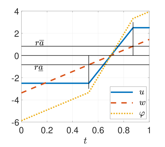
We note that the optimal primal solution is unique, no matter what the value of , or , is, of course (see Fact 2). On the other hand, the optimal dual solution depends on the parameter : as changes the slope of the line representing the graph of changes with the -intercept remaining the same. The fixed point also evolves to obey . For a fixed we cannot prove that is unique but after running Algorithm 1 with using randomly generated starting points we always converged to the same .
5.2 Machine tool manipulator
A machine tool manipulator is a machine used to simulate human hand movements usually found in manufacturing. In [13, 11] this is modelled as an optimal control problem of the form in (2) with
, , . We alter the objective function given in the previously mentioned references to be the minimum-energy control as in [10]. As with the double integrator problem we cannot solve this problem analytically hence the need for a numerical method such as the one in this paper. The projector onto is as given in Fact 5 with . Due to the large number of state variables involved in this problem it is not feasible to give the projector onto in closed form so we implement a numerical approach to approximate the projector. The numerical algorithm and expression for the projector onto are given in [10].
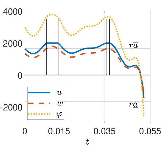
For this problem let , , (i.e., ). The value of will not impact the solution but from experiments in [10], had the fastest performance. With and Algorithm 1 converged in 249 iterations. From Figure 2 we can again observe that, as stated in Theorem 2, . We can also see that Condition (49) is verified by the plots in Figure 2 which once more confirms the optimality of .
6 Conclusion
We have explored relationships between the primal and dual optimal control problems as the DR algorithm is applied to solve them. We derived the Fenchel dual to the primal problem. We provided an explicit expression of the set of fixed points of the DR operator as the Minkowski sum of the sets of primal and dual solutions. We showed that the fixed point expression can be used as a certificate of optimality in that the optimality conditions for optimal control obtained numerically can be checked.
As an example, we first chose the minimum-energy control of the double integrator, which is simple yet rich enough to illustrate the concepts we developed and the results we obtained. We also applied our methodology to the minimum-energy control of a machine tool manipulator model which is numerically more challenging to solve than the double integrator.
In the future, the work we did here should be extended to general LQ optimal control problems, also involving constraints on the state variables. We considered only constraints on the control variables in the present paper. The inclusion of state variable constraints is well known to create theoretical and numerical challenges. The derivation of the dual of LQ control problems, albeit in a space different to that of the primal, done in [1, 11] involves only constraints on the control variables, so the work there needs to be extended first.
Acknowledgments
The authors are indebted to the two anonymous reviewers whose comments and suggestions improved the paper. The research of BIC is supported by an Australian Government Research Training Program Scholarship, as well as by the funding provided by the Universities of South Australia and Waterloo for her three-month visit to the University of Waterloo. The research of WMM is supported by the Natural Sciences and Engineering Research Council of Canada Discovery Grant and the Ontario Early Researcher Award.
References
- [1] W. Alt, C. Y. Kaya, and C. Schneider, Dualization and discretization of linear-quadratic problems with bang–bang solutions. EURO J. Comput. Optim., 4 (2016), 47–77.
- [2] H. M. Amman, D. A. Kendrick, Computing the steady state of linear quadratic optimization models with rational expectations. Econ. Lett., 58(2), 185–191, 1998.
- [3] M. Athans and P. Falb, Optimal Control: An Introduction to the Theory and Its Applications. McGraw-Hill, Inc., New York, 1966.
- [4] H. Attouch, M. Thera, A general duality principle for the sum of two operators. J. Convex Anal. 3 (1996), 1–24.
- [5] H. H. Bauschke, R. S. Burachik, and C. Y. Kaya, Constraint splitting and projection methods for optimal control of double integrator. In: H. H. Bauschke, R. S. Burachik and D. R. Luke, “Splitting Algorithms, Modern Operator Theory, and Applications,” Springer Nature, Switzerland, pp. 45–68, 2019.
- [6] H. H. Bauschke, W. L. Hare, and W. M. Moursi, Generalized solutions for the sum of two maximally monotone operators. SIAM J. Control Optim., 52 (2014), 1034–1047.
- [7] H. H. Bauschke, R. I. Boţ, W. L. Hare, and W. M. Moursi, Attouch–Thera duality revisited: paramonotonicity and operator splitting. J. Approx. Theory, 164 (2012), 1065–1084.
- [8] H. H. Bauschke and P. L. Combettes, Convex Analysis and Monotone Operator Theory in Hilbert Spaces. 2nd edition, Springer, 2017.
- [9] A. V., Bulatov and V. F. Krotov, On dual problems of optimal control. Automat. Rem. Contr., 69 (2008), pp. 1653–1662.
- [10] R. S. Burachik, B. I. Caldwell, and C. Y. Kaya, Projection methods for control-constrained minimum-energy control problems. arXiv:2210.17279v1, https://arxiv.org/abs/2210.17279.
- [11] R. S. Burachik, C. Y. Kaya, and S. N. Majeed, A duality approach for solving control-constrained linear-quadratic optimal control problems. SIAM J. Control Optim., 52 (2014), 1771–1782.
- [12] C. Büskens, H. Maurer, SQP-methods for solving optimal control problems with control and state constraints: Adjoint variables, sensitivity analysis and real-time control. J. Comput. Appl. Math., 120(1), 85–108, 2000.
- [13] B. Christiansen, H. Maurer, and O. Zirn, Optimal control of machine tool manipulators. Recent Advances in Optimization and its Applications in Engineering, Springer-Verlag, Berlin, Heidelberg, 2010.
- [14] F. Clarke, Functional Analysis, Calculus of Variations and Optimal Control. Springer-Verlag, London, 2013.
- [15] R. Fourer, D. M. Gay, and B. W. Kernighan, AMPL: A Modeling Language for Mathematical Programming, Second Edition. Brooks/Cole Publishing Company / Cengage Learning, 2003.
- [16] J. Eckstein, Splitting Methods for Monotone Operators with Applications to Parallel Optimization. Ph.D. thesis, MIT, 1989.
- [17] W. W. Hager and G. D. Ianculescu, Dual approximations in optimal control. SIAM J. Control Optim., 22 (1984), 423–465.
- [18] M. R. Hestenes, Calculus of Variations and Optimal Control Theory. John Wiley & Sons, New York, 1966.
- [19] C. Y. Kaya, Optimal control of the double integrator with minimum total variation. J. Optim. Theory Appl., 185 (2020), 966–981.
- [20] D. E. Kirk, Optimal Control Theory: An Introduction. Prentice-Hall, Inc., New Jersey, 1970.
- [21] J. Klamka, Controllability and Minimum Energy Control. Springer, Cham, Switzerland, 2019.
- [22] B. Kugelmann, H. J. Pesch, New general guidance method in constrained optimal control, part 1: Numerical method. J. Optim. Theory Appl., 67(3), 421–435, 1990.
- [23] A. Locatelli, Optimal Control of a Double Integrator: A Primer on Maximum Principle. Springer, Switzerland, 2017.
- [24] H. Maurer, H. J. Oberle, Second order sufficient conditions for optimal control problems with free final time: The Riccati approach. SIAM J. Control Optim., 41 (2), 380–403, 2003.
- [25] T. Mouktonglang, Innate immune response via perturbed LQ-control problem. Adv. Stud. Biol., 3, 327–332, 2011.
- [26] B. S. Mordukhovich, Variational Analysis and Generalized Differentiation II: Applications. Springer-Verlag, Berlin, Heidelberg, 2006.
- [27] B. O’Donoghue, G. Stathopoulos, and S. Boyd, A splitting method for optimal control. IEEE Trans. Contr. Sys. Tech., 21, 2432–2442, 2013.
- [28] L. S. Pontryagin, V. G. Boltyanskii, R. V. Gamkrelidze, and E. F. Mishchenko, The Mathematical Theory of Optimal Processes. John Wiley & Sons, New York, 1962.
- [29] R. T. Rockafellar, Conjugate convex functions in optimal control and the calculus of variations. J. Convex Anal. Appl., 32 (1970), 174–222.
- [30] R. T. Rockafellar, Existence and duality theorems for convex problems of Bolza. Trans. Amer. Math. Soc., 159 (1971), 1–40.
- [31] R. T. Rockafellar, Linear quadratic programming and optimal control. SIAM J. Control Optim., 25 (1987), 781–814.
- [32] W. J. Rugh, Linear System Theory, 2nd Edition. Pearson, 1996.
- [33] S. P. Sethi, Optimal Control Theory: Applications to Management Science and Economics, First Edition. Springer, Cham, Switzerland, 2019.
- [34] R. B. Vinter, Optimal Control, Birkhäuser, Boston, 2000.
- [35] A. Wächter and L. T. Biegler, On the implementation of a primal-dual interior point filter line search algorithm for large-scale nonlinear programming. Math. Progr., 106 (2006), 25–57.