Two-dimensional reductions of the Whitham modulation system for the Kadomtsev-Petviashvili equation

Optical Kerr spatiotemporal dark-lump dynamics of hydrodynamic origin

Line soliton interactions of the Kadomtsev-Petviashvili equation

Soliton solutions of the Kadomtsev-Petviashvili II equation

Towards an inverse scattering theory for non-decaying potentials of the heat equation

Extended resolvent and inverse scattering with an application to KPI

Building an extended resolvent of the heat operator via twisting transformations

On the equivalence of different approaches for generating multisoliton solutions of the KPII equations

Thèorie Des Ondes et Des Remous Qui Se Propagent Le Long d’un Canal Rectangulaire Horizontal, En Communiquant Au Liquide Contenu Dans Ce Canal Des Vitesses Sensiblement Pareilles de La Surface Au Fond

Dispersive shock waves and modulation theory

On the stability of solitary waves in weakly dispersive media

Ion acoustic soliton experiments in a plasma

Self-focusing of plane dark solitons in nonlinear defocusing media

Stability of magnetoelastic solitons and self-focusing of sound in antiferromagnet

The direct scattering problem for perturbed Kadomtsev-Petviashvili multi line solitons

Stability of Kadomtsev-Petviashvili multi-line solitons

Abstract

Two-dimensional reductions of the KP-Whitham system, namely the overdetermined Whitham modulation system for five dependent variables that describe the periodic solutions of the Kadomtsev-Petviashvili equation, are studied and characterized. Three different reductions are considered corresponding to modulations that are independent of $x$, independent of $y$, and of $t$ (i.e., stationary), respectively. Each of these reductions still describes dynamic, two-dimensional spatial configurations since the modulated cnoidal wave generically has a nonzero speed and a nonzero slope in the $xy$ plane. In all three of these reductions, the properties of the resulting systems of equations are studied. It is shown that the resulting reduced system is not integrable unless one enforces the compatibility of the system with all conservation of waves equations (or considers a reduction to the harmonic or soliton limit). In all cases, compatibility with conservation of waves yields a reduction in the number of dependent variables to two, three and four, respectively. As a byproduct of the stationary case, the Whitham modulation system for the Boussinesq equation is also explicitly obtained.

1 Introduction and background

The description of dispersive wave propagation has been a classical topic of study dating back to the works of Boussinesq, Stokes, Rayleigh, Korteweg and de Vries and others in the nineteenth century, and it continues to attract significant attention. A scenario of both theoretical and applicative interest is that in which dispersive effects are much smaller than nonlinear ones, a regime that often leads to the generation of dispersive shock waves. Indeed, a large number of works have been devoted to this subject (e.g., see [17] and references therein). The mathematical framework for the description of small dispersion problems in one spatial dimension and the formation of dispersive shock waves in that context have been well characterized, beginning with the seminal work of G. B. Whitham [36]. However, our understanding of dispersive wave propagation and dispersive shock waves in more than one spatial dimension is much less developed.

The purpose of this work is to study special solutions of the Kadomtsev-Petviashvili (KP) equation [23],

$$(u_{t}+6uu_{x}+\varepsilon^{2}u_{xxx})_{x}+\sigma u_{yy}=0\,,$$ (1.1)

where $0<\varepsilon\ll 1$, subscripts $x$, $y$ and $t$ denote partial differentiation and the values $\sigma=\mp 1$ distinguish between the KPI and KPII variants of the KP equation, respectively. The KP equation, which is a two-dimensional generalization of the celebrated Korteweg-de Vries (KdV) equation, similarly arises in such diverse fields as plasma physics [22, 23, 26], fluid dynamics [6, 24], nonlinear optics [7, 29] and ferromagnetic media [34]. The KP equation is also, like the KdV equation, a completely integrable infinite-dimensional Hamiltonian system whose solutions possess a rich mathematical structure [5, 8, 21, 22, 24, 25, 27]. The initial-value problem for the KP equation is in principle amenable to exact solution via the inverse scattering transform (IST) [5, 25, 27]. Yet, even though considerable work has been devoted to the development of the IST for the KP equation throughout the last twenty years [12, 13, 14, 15, 37], the IST has rarely been used to study the dynamical behavior of solutions of the KP equation [38]. Conversely, asymptotic methods such as Whitham modulation theory have recently been shown to be quite effective in this regard [4, 11, 30, 32].

In this work, we derive and characterize several asymptotic reductions of the KP equation, which we rewrite in evolution form as

$$u_{t}+6uu_{x}+\varepsilon^{2}u_{xxx}+\sigma v_{y}=0\,,\qquad v_{x}=u_{y}\,.$$ (1.2)

The linear dispersion relation of (1.2), obtained by looking for small-amplitude plane-wave solutions $u(x,y,t)=u_{o}+A\,e^{i\theta(x,y,t)}$ with $|A|\ll|u_{o}|$, $\theta(x,y,t)=(kx+ly-\omega t)/\varepsilon$, is $\omega=(6u_{o}+\sigma q^{2})k-k^{3}$, with $q=l/k$. In addition, the KP equation admits nonlinear, exact traveling wave solutions in the form of “cnoidal waves”

$$u(x,y,t)=r_{1}-r_{2}+r_{3}+2(r_{2}-r_{1})\mathop{\rm cn}\nolimits^{2}(2\theta K_{m};m)\,,\qquad v(x,y,t)=qu+p\,,$$ (1.3)

where $\mathop{\rm cn}\nolimits(\cdot)$ denotes the Jacobian elliptic cosine [28], $K_{m}=K(m)$ and $E_{m}=E(m)$ are the complete elliptic integrals of the first and second kind, respectively, and

$$m=\frac{r_{2}-r_{1}}{r_{3}-r_{1}}$$ (1.4)

is the elliptic parameter. The above solution is completely determined by five parameters: $r_{1}$, $r_{2}$, $r_{3}$, $q$ and $p$. The local wavenumber $k$ and $l$ in the $x$ and $y$ directions and the frequency $\omega$ are then obtained as

$$k={\sqrt{r_{3}-r_{1}}}\,\big{/}{2K_{m}}\,,$$ (1.0a)

$$l=qk\,,$$ (1.0b)

$$\omega=(V+\sigma q^{2})k\,,$$ (1.0c)

with

$$V=\frac{\omega}{k}-\sigma q^{2}=2(r_{1}+r_{2}+r_{3})\,.$$ (1.1)

In [4], the method of multiple scales was used to derive the so-called KP-Whitham system, i.e., a system of quasilinear first-order PDEs that describes the slow modulation of the above periodic solutions of the KP equation. One begins by seeking a solution of (1.2) in the form $u=u(\theta,x,y,t)$, with rapidly varying variable $\theta(x,y,t)$ defined through its derivatives:

$$\theta_{x}={k(x,y,t)}/{\varepsilon},\qquad\theta_{y}={l(x,y,t)}/{\varepsilon},\qquad\theta_{t}=-{\omega(x,y,t)}/{\varepsilon}\,.$$ (1.2)

Here, $k(x,y,t)$ and $l(x,y,t)$ are the local wave numbers in the $x$ and $y$ directions, respectively, and $\omega(x,y,t)$ is the wave’s local frequency. Imposing the equality of the mixed second derivatives of $\theta$ results in the compatibility conditions

$$k_{t}+\omega_{x} =0\,,$$ (1.0a)

$$l_{t}+\omega_{y} =0\,,$$ (1.0b)

$$k_{y}-l_{x} =0\,,$$ (1.0c)

called the “conservation of waves” equations. One also introduces the dependent variable

$$q(x,y,t)=\frac{l}{k}\,$$ (1.1)

consistent with the above periodic solutions, along with the slowly varying variables $x$, $y$ and $t$. It was then shown in [4] that to leading order one recovers the solution (1.3). When the parameters of the above periodic solution are slowly modulated with respect to $x$, $y$ or $t$, they satisfy a system of Whitham modulation equations. When writing down these equations, it is convenient to define the “convective derivative”

$$\frac{D}{Dy}{}=\frac{\partial}{\partial{y}}-q\frac{\partial}{\partial{x}}~{}.$$ (1.2)

In component form, the KP-Whitham system (KPWS) is then comprised of the following partial differential equations (PDEs)

$$\frac{\partial r_{i}}{\partial{t}}+(V_{j}+\sigma q^{2})\frac{\partial r_{j}}{\partial{x}}+2\sigma q\frac{Dr_{j}}{Dy}+\sigma\nu_{j}\frac{Dq}{Dy}+\sigma\frac{Dp}{Dy}=0\,,\qquad j=1,2,3,$$ (1.0a)

$$\frac{\partial q}{\partial{t}}+(V_{2}+\sigma q^{2})\frac{\partial q}{\partial{x}}+2\sigma q\frac{Dq}{Dy}+(4-\nu_{4})\frac{Dr_{1}}{Dy}+(2+\nu_{4})\frac{Dr_{3}}{Dy}=0\,,$$ (1.0b)

$$\frac{\partial p}{\partial{x}}-(1-\alpha)\frac{Dr_{1}}{Dy}-\alpha\frac{Dr_{3}}{Dy}+\nu_{5}\frac{\partial q}{\partial{x}}=0\,,$$ (1.0c)

$$b_{1}\frac{Dr_{1}}{Dy}+b_{2}\frac{Dr_{2}}{Dy}+b_{3}\frac{Dr_{3}}{Dy}+b_{4}\frac{\partial q}{\partial{x}}=0\,.$$ (1.0d)

[Note that (1.0a) is a consequence of the three equations (1.0a), while (1.0b) and (1.0c) are equivalent to (1.0b) and (1.0d), respectively.] Here, $V_{1},\dots,V_{3}$ are the characteristic speeds of the Whitham system for the KdV equation, namely

$$V_{1}=V-2b\frac{K_{m}}{K_{m}-E_{m}}\,,\quad V_{2}=V-2b\frac{(1-m)K_{m}}{E_{m}-(1-m)K_{m}}\,,\quad V_{3}=V+2b\frac{(1-m)K_{m}}{mE_{m}}\,,$$

and $b=2(r_{2}-r_{1})$ is the amplitude of the cnoidal wave solution (1.3), while the remaining coefficients are

$$\nu_{1}=\frac{V}{6}+\frac{b}{3m}\frac{(1+m)E_{m}-K_{m}}{K_{m}-E_{m}}\,,\quad\nu_{2}=\frac{V}{6}+\frac{b}{3m}\frac{(1-m)^{2}K_{m}-(1-2m)E_{m}}{E_{m}-(1-m)K_{m}}\,,$$ (1.0a)

$$\nu_{3}=\frac{V}{6}+\frac{b}{3m}\frac{(2-m)E_{m}-(1-m)K_{m}}{E_{m}}\,,\quad\nu_{4}=\frac{2mE_{m}}{E_{m}-(1-m)K_{m}}\,,$$ (1.0b)

$$\nu_{5}=r_{1}-r_{2}+r_{3}\,,\quad\alpha=\frac{E_{m}}{K_{m}}\,,\quad b_{1}=(1-m)(K_{m}-E_{m}),$$ (1.0c)

$$b_{2}=E_{m}-(1-m)K_{m},\quad b_{3}=-mE_{m},\quad b_{4}=2(r_{2}-r_{1})(1-m)K_{m}$$ (1.0d)

Importantly, the modulation system (1.2) contains six PDEs for the five dependent variables $r_{1}$, $r_{2}$, $r_{3}$, $q$ and $p$, and is therefore overdetermined in general. In [4], the initial value problem for the system (1.2) was shown to be compatible provided that (1.0c) and (1.0d) hold at $t=0$, in which case it was shown that (1.0c) and (1.0d) remain satisfied for all $t>0$. Consequently, in [4] a reduced system consisting of the five PDEs (1.0a)–(1.0c) was considered, which is a minimal set of equations for the five dependent variables ${\mathbf{r}}=(r_{1},r_{2},r_{3},q,p)^{T}$ that can be written as

$$I_{4}\,\frac{\partial{\mathbf{r}}}{\partial{t}}+A_{5}\,\frac{\partial{\mathbf{r}}}{\partial{x}}+B_{5}\,\frac{\partial{\mathbf{r}}}{\partial{y}}=0\,,$$ (1.1)

where $I_{4}=\mathop{\rm diag}\nolimits(1,1,1,1,0)$ and $A_{5}$ and $B_{5}$ are $5\times 5$ matrices whose explicit form is given in (A.1). In [4] and [11] the term “KP-Whitham system” was used to refer to the five equations (1.1). However, in this work we will show that, in order for the modulation system to inherit the integrability properties of the KP equation, it is crucial to consider all six equations (1.2) on an equal footing. Accordingly, we will henceforth refer to the system (1.1) as the “original KPWS”, and we will refer to the six equations (1.2) as the “full KPWS”.

Generally, all the dependent variables in (1.2) depend on two spatial dimensions ($x$ and $y$) and one temporal dimension ($t$), so we refer to the KPWS (1.2) as $(2+1)$-dimensional, or equivalently 3-dimensional. A number of asymptotic reductions of the system (1.2) and their properties were studied in [11], and $(1+1)$-dimensional (i.e., 2-dimensional) reductions of the soliton limit of (1.2) were used in [30, 31, 32] to study various concrete physical problems. A number of important questions remain open, however. Among them is the issue of integrability. Since the KP-Whitham system was derived as an exact asymptotic reduction of the KP equation (1.1), which is integrable, one would naturally expect that the modulation system is also integrable. On the other hand, as was mentioned in [4], the system (1.2a–c) fails the Haantjes tensor test for integrability [19]. At the same time, it was shown in [11] that the harmonic and soliton limits of the system (1.2) are in fact integrable. An obvious question is then whether there are other integrable reductions of (1.2) and if so how one can identify them.

In this work, we begin to address this question by studying and characterizing the two-dimensional ($1+1$ and $2+0$) reductions of the KPWS (1.2). We demonstrate that these reductions of the original KPWS are integrable only if the full KPWS is compatible. In section 2 we consider the situation in which all fields are independent of $x$, and in section 3 the situation in which all fields are independent of $y$. In section 4 we study the situation in which all fields are stationary, i.e., independent of $t$. Finally, in section 5 we discuss the compatbility of the full KPWS, and in section 6 we conclude this work with some final remarks. We emphasize that, as in [30, 32, 31], even when the solution of the KPWS is independent of one independent variable, the reduced systems of equations still generically describe two-dimensional, dynamical configurations of the KP equation, because nonzero $V$ (1.1) implies propagation of the cnoidal wave and $q$ describes the orientation of the periodic wave in the $xy$ plane. Variations of $q$ with respect to $x$ or $y$ correspond to curved wave profiles. Section 6 ends this work with some concluding remarks.

To avoid confusion, we note that in this work we are using the normalization of [4], not that of [11, 31, 30, 32]. In the latter works, the coefficient 6 in front of the term $uu_{x}$ in (1.2) was absent and the cnoidal wave’s period was normalized to $2\pi$, whereas here it is normalized to unity. As a result, several formulas are adjusted accordingly.

2 The YT system

In this section we consider solutions of the KPWS in which all fields are independent of $x$. We begin by considering the original KPWS (1.1) [i.e., the five-component system (1.2a–c)], neglecting the compatibility condition (1.0d) at first. When solutions are independent of $y$, (1.1) reduces to a system of five PDEs in the independent variables $y$ and $t$, which we refer to as the “YT system”. In vector form, this YT system is

$$I_{4}\frac{\partial{\mathbf{r}}}{\partial{t}}+B_{5}\frac{\partial{\mathbf{r}}}{\partial{y}}=0\,,$$ (2.1)

where ${\mathbf{r}}=(r_{1},r_{2},r_{3},q,p)^{T}$ and $I_{4}=\mathop{\rm diag}\nolimits(1,1,1,1,0)$ as before, and the coefficient matrix $B_{5}$ is given in (A.0l).

2.1 Reduction of the YT system to a three-component system

The number of equations in the system (2.1) can be reduced through a suitable change of variables. Explicitly, the last row of (2.1) is

$$\frac{\partial r_{1}}{\partial{y}}+\alpha\frac{\partial}{\partial{y}}(r_{3}-r_{1})=0\,.$$ (2.2)

Then, we use the transformation

$$s_{1}=r_{3}-r_{2}\,,\quad s_{2}=r_{3}-r_{1}\,,\quad s_{3}=r_{2}-r_{1}\,$$ (2.3)

where we made the choice not to define these variables in cyclic fashion in order to preserve the property that $s_{j}\geq 0$ $\forall j=1,2,3$ when the Riemann-type variables $r_{1},\dots,r_{3}$ are well-ordered. This transformation leads to the set of equations

$$\frac{\partial s_{j}}{\partial{t}}+2\sigma q\frac{\partial s_{j}}{\partial{y}}+\sigma\Delta\nu_{j}\frac{\partial q}{\partial{y}}=0\,,\quad j=1,2,3,$$ (2.0a)

$$\frac{\partial q}{\partial{t}}+6\frac{\partial r_{1}}{\partial{y}}+(\nu_{4}+2)\frac{\partial s_{2}}{\partial{y}}+2\sigma q\frac{\partial q}{\partial{y}}=0\,,$$ (2.0b)

with $\Delta\nu_{1}=\nu_{3}-\nu_{2}$, $\Delta\nu_{2}=\nu_{3}-\nu_{1}$ and $\Delta\nu_{3}=\nu_{2}-\nu_{1}$. The transformation (2.3) is not invertible. However, (2.0a) with $j=1$ is decoupled from the rest of the system, since $s_{1}$ does not appear in the remaining equations. Thus we can simply disregard it moving forward, since the four dependent variables $r_{1}$, $s_{2}$, $s_{3}$ and $q$, determined by the PDEs (2.0a) with $j=2,3$ plus (2.0b), are a closed system. These dependent variables, together with (2.2), are sufficient to recover the solution of the KP equation.

Next, one can use (2.2) to eliminate $r_{1}$ from (2.0b), obtaining the following closed system of three PDEs for the three dependent variables $s_{2}$, $s_{3}$ and $q$:

$$\frac{\partial s_{2}}{\partial{t}}+2\sigma q\frac{\partial s_{2}}{\partial{y}}+\sigma(\nu_{3}-\nu_{1})\frac{\partial q}{\partial{y}}=0\,,$$ (2.0a)

$$\frac{\partial s_{3}}{\partial{t}}+2\sigma q\frac{\partial s_{3}}{\partial{y}}+\sigma(\nu_{2}-\nu_{1})\frac{\partial q}{\partial{y}}=0\,,$$ (2.0b)

$$\frac{\partial q}{\partial{t}}+(\nu_{4}-6\alpha+2)\frac{\partial s_{2}}{\partial{y}}+2\sigma q\frac{\partial q}{\partial{y}}=0\,,$$ (2.0c)

All the coefficients appearing in (2.1) are completely determined by $m$ and $b$, which in turn are completely determined by $s_{2},s_{3}\&q$ as

$$m=\frac{s_{3}}{s_{2}}\,,\qquad\frac{b}{m}=2s_{2}\,.$$ (2.1)

Note that $r_{1}$ is also needed to recover the asymptotic solution of the KP equation, but its value, up to an integration constant determined by the initial conditions, can be obtained from $s_{2}$, $s_{3}$ by integrating (2.2). Introducing the vector ${\mathbf{v}}=(s_{2},s_{3},q)^{T}$, we can write the above system (2.1) in vector form as

$$\frac{\partial{\mathbf{v}}}{\partial{t}}+B_{3}\frac{\partial{\mathbf{v}}}{\partial{y}}=0\,,$$ (2.2)

with

$$B_{3}=\left(\begin{array}[]{ccc}2\sigma q&0&\sigma(\nu_{3}-\nu_{1})\\ 0&2\sigma q&\sigma(\nu_{2}-\nu_{1})\\ \nu_{4}-6\alpha+2&0&2\sigma q\end{array}\right)\,.$$ (2.3)

The eigenvalues of $B_{3}$ are

$$\lambda_{1}=2\sigma q,\qquad\lambda_{2,3}=2\sigma q\pm\sqrt{\Delta}\,,$$ (2.0a)

where

$$\Delta=\sigma\left(\nu_{1}-\nu_{3}\right)\left(6\alpha-\nu_{4}-2\right)=4\sigma s_{2}\frac{((1-m)K_{m}-2(2-m)E_{m}K_{m}+3E_{m}^{2})^{2}}{3E_{m}K_{m}(K_{m}-E_{m})(E_{m}-(1-m)K_{m})}\,.$$ (2.0b)

By properties of $K_{m}$ and $E_{m}$, $\mathop{\rm sgn}\nolimits\Delta=\mathop{\rm sgn}\nolimits\sigma$ since $s_{2}>0$. Hence, if $\sigma=-1$, as for KPI, some of the eigenvalues are imaginary, implying that the initial value problem for the above system is ill-posed, confirming known results [4]. Incidentally, note that the PDEs for $s_{2}$ and $q$ do not contain $s_{3}$ explicitly. However, the value of $s_{3}$ is required to determine $m$.

2.2 Harmonic and soliton limits of the YT system

We now consider two distinguished limits of the system outlined in (2.0a), which describe concrete physical scenarios: the harmonic limit and the soliton limit. The limiting values of all coefficients of the KPWS in these limits are found in the Appendix.

The harmonic limit, in which the elliptic parameter $m\to 0$, is obtained by taking $r_{2}\to r_{1}^{+}$. In this limit, the cnoidal wave becomes a vanishing-amplitude trigonometric wave (cf. section 1 and the well-known properties of the elliptic functions [28]). Note $s_{3}\to 0$ in this limit, consistent with the fact that $m$ is obtained from $s_{2}$ and $s_{3}$ via (2.1). The harmonic limit of system (2.0a) results in the partially decoupled system

$$\frac{\partial s_{2}}{\partial{t}}+2\sigma q\frac{\partial s_{2}}{\partial{y}}=0\,,$$ (2.0a)

$$\frac{\partial q}{\partial{t}}+2\sigma q\frac{\partial q}{\partial{y}}=0\,,$$ (2.0b)

with identical equations for the variables $s_{2}\&q$. In the limit $m\to 0$ of (1.3), the mean flow is simply $\bar{u}=r_{3}$. Moreover, (2.2) implies that, in the harmonic limit, $\partial{r_{3}}/\partial{y}\to 0$. Thus the mean flow is constant with respect to all spatial variables, but it does not play any role in the system. Moreover, taking into account the reduction of (2.2), we see that the system (2.2) coincides with the harmonic limits in [11] and [4] when derivatives with respect to $x$ are neglected.

The soliton limit, i.e., $m\to 1$, is obtained when $r_{2}\to r_{3}^{-}$, which amounts to $s_{3}\to s_{2}$, and the cnoidal wave solution (1.3) limiting to a line soliton. The first two equations of (2.2) are identical in this limit, consistent with $s_{3}=s_{2}$, while the remaining equations are

$$\frac{\partial s_{2}}{\partial{t}}+2\sigma q\frac{\partial s_{2}}{\partial{y}}+\frac{4}{3}\sigma s_{2}\frac{\partial q}{\partial{y}}=0$$ (2.0a)

$$\frac{\partial q}{\partial{t}}+4\frac{\partial s_{2}}{\partial{y}}+2\sigma q\frac{\partial q}{\partial{y}}=0\,.$$ (2.0b)

As before, (2.2) coincides with the reduction of the soliton limit in [4] and [11] when derivatives with respect to $x$ are neglected. In this case, since $\alpha\to 0$ as $m\to 1$, (2.2) implies $\partial r_{1}/\partial y=0$ and $\partial{s_{2}}/\partial{y}=\partial{r_{3}}/\partial{y}$. Unlike the harmonic limit, the two-component system (2.2) in the soliton limit is coupled. On the other hand, the system can be diagonalized in a straightforward way. The eigenvalues of the system and the associated left eigenvectors are, respectively [11],

$$\lambda_{\pm}=2\sigma q\pm 4\sqrt{{\sigma s_{2}}/{3}}\,,\qquad{\mathbf{w}}_{\pm}=(\pm\sqrt{3},\sqrt{\sigma s_{2}})\,.$$ (2.1)

Using these, we obtain the characteristic differential forms $\sqrt{3}{\rm d}s_{2}\pm\sqrt{\sigma s_{2}}{\rm d}q=\sqrt{3\sigma/s_{2}}{\rm d}s_{2}\pm{\rm d}q=0$, which yields the Riemann invariants

$$R_{\pm}=q\pm 2\sqrt{3\sigma s_{2}}\,.$$ (2.2)

In turn, the change of variable from $s_{2}$ and $q$ to $R_{\pm}$ transforms the system (2.2) into diagonal form:

$$\frac{\partial R_{\pm}}{\partial{t}}+\lambda_{\pm}\frac{\partial R_{\pm}}{\partial{x}}=0\,.$$ (2.3)

2.3 Integrability and Riemann invariant of the YT system

We now return to the three-component YT system (2.2). The Haantjes tensor test for integrability of a system of hydrodynamic equations [19] (see also the Appendix) is a relatively simple way to determine whether a strictly hyperbolic system is diagonalizable. It is generally believed that asymptotic reductions of an integrable system preserve integrability. While the KP equation (1.2) is integrable, the five-component original KP Whitham system (1.2a–c) fails the Haantjies tensor test, a necessary condition for the integrability of three-dimensional quasi-linear systems [18]. At the same time, it was shown in [11] that the three-dimensional harmonic and soliton limits of the full system are indeed integrable, which then raises the natural question of whether two-dimensional reductions of the KPWS are integrable.

The three-component YT system (2.2) fails the Haantjes tensor test, since 19 out of the 27 components of the Haantjes tensor vanish in general. The Haantjes tensor does vanish in the limit $m\to 0$, but its entries diverge in the limit $m\to 1$, even though, as we showed above, the limiting system can be reduced to an integrable two-component system for $s_{2}$ and $q$.

The reason for this discrepancy, and the reason why the original KPWS and the reduction (2.2) fails the Haantjes tensor test is that, in order for (1.2) or (1.1) to be compatible, $q$ and $k$ must be related by condition (1.0c), i.e., $k_{y}=l_{x}$, or, equivalently, (1.2d). When the initial conditions do not satisfy the compatibility condition (1.2d), the original KPWS does not describe actual solutions of the KP equation, and that explains why the original KPWS system may not be integrable despite the integrability of the KP equation. Indeed, we show below that, once the compatibility condition $k_{y}=l_{x}$ is enforced, the $x$-independent reduction of the full KPWS (the YT system) is in fact integrable. Later, in sections 3 and 4, we will see how similar considerations apply to the $y$-independent and $t$-independent reductions of the KPWS.

The coefficient matrix $A$ in (A.0l) has the eigenvalue $2\sigma q$, which is inherited by the matrix $B$ in (2.3). Using the corresponding left eigenvector in (2.3), we have the following characteristic relation

$$(\nu_{2}-\nu_{1}){\rm d}s_{2}-(\nu_{3}-\nu_{1}){\rm d}s_{3}=0\,,$$ (2.4)

along ${\rm d}y/{\rm d}t=2\sigma q$. To integrate this differential form, we eliminate $s_{3}$ in favor of $m$ using (2.1), to obtain

$$(\nu_{2}-\nu_{1}-m(\nu_{3}-\nu_{1}))\,{\rm d}s_{2}-s_{2}(\nu_{3}-\nu_{1})\,{\rm d}m=0\,.$$ (2.5)

Multiplying by the integrating factor $1/[s_{2}(\nu_{2}-\nu_{1}-m(\nu_{3}-\nu_{1}))]$ yields

$$\frac{1}{s_{2}}{\rm d}s_{2}+\bigg{(}\frac{1}{m}-\frac{E_{m}}{m(1-m)K_{m}}\bigg{)}{\rm d}m=0\,,$$ (2.6)

and recalling the derivative of $K_{m}$ [cf. (A.0a)], we express the above characteristic relation as

$${\rm d}\big{[}\frac{1}{2}\log s_{2}-\log K_{m}\big{]}=0,$$ (2.7)

which yields the Riemann invariant $R_{o}={\sqrt{s_{2}}}\,\big{/}{2K_{m}}$ that satisfies the PDE

$$\frac{\partial R_{o}}{\partial{t}}+2\sigma q\frac{\partial R_{o}}{\partial{y}}=0\,.$$ (2.8)

In light of (1.0a) and (2.3), however, we see that $R_{o}\equiv k$! That is, the Riemann invariant $R_{o}$ is just the local wavenumber $k$ in the $x$ direction. Moreover, the fact that $k$ is a Riemann invariant is deeply connected with the integrability of the full KPWS. This is because, when all fields are independent of $x$, the conservation of waves and compatibility condition (1.2) immediately yield $k_{t}=k_{y}=0$, i.e., $k={}$const. Enforcing the constancy of the local wavenumber $k$ (as needed to ensure the compatibility of the full KPWS with the KP equation, as per the above discussion) reduces the three-component YT system (2.2) to a two-component system that is locally integrable. Any two-component system can always be reduced to Riemann invariant form and is therefore always locally integrable via the classical hodograph transform. We will see in sections 3 and 4 that a similar phenomenon will also arise for the $y$-independent and $t$-independent reductions of the KPWS.

2.4 Further reduction of the YT system and its diagonalization

Since the wavenumber $k$ is simultaneously a Riemann invariant of the three-component YT system (2.2) and a conserved quantity for $x$-independent one-phase solutions of the KP equation, we now derive a reduction of the YT system in which $k$ is constant. We choose two different sets of dependent variables: a reduced system for the dependent variables $(s_{2},q)^{T}$ and the reduced system for the dependent variables $(m,q)^{T}$.

We begin by performing a change of variable from ${\mathbf{v}}=(s_{2},s_{3},q)^{T}$ to ${\tilde{\mathbf{v}}}=(s_{2},q,k)^{T}$. We choose to keep $s_{2}$ as opposed to $s_{3}$ because $s_{2}$ never vanishes, whereas $s_{3}\to 0$ in the harmonic limit. Then ${\tilde{\mathbf{v}}}$ satisfies the system ${\tilde{\mathbf{v}}}_{t}+{\tilde{B}}_{3}\,{\tilde{\mathbf{v}}}_{y}=0$, with ${\tilde{B}}_{3}=T^{-1}B_{3}T$ and $T=\big{(}{\partial v_{i}}/{\partial{\tilde{v}}_{j}}\big{)}$ . One can verify that the new coefficient matrix is block-diagonal, ${\tilde{B}}_{3}=\mathop{\rm diag}\nolimits(B_{2},2\sigma q)$, with the $2\times 2$ matrix $B_{2}$ given by

$$B_{2}=\left(\!\begin{array}[]{cc}2\sigma q&2\sigma s_{2}\displaystyle\frac{(1-m)K_{m}^{2}-2(2-m)K_{m}E_{m}+3E_{m}^{2}}{3E_{m}(E_{m}-K_{m})}\\ \displaystyle 2+2\left(\frac{m}{E_{m}-(1-m)K_{m}}-\frac{3}{K_{m}}\right)E_{m}&2\sigma q\end{array}\!\right)\,.$$ (2.11)

(2.12)

Since compatibility of the KPWS requires $k_{t}=k_{y}=0$, we therefore consider the compatible solution $k\equiv{}$const, which simplifies the $3\times 3$ system ${\tilde{\mathbf{v}}}_{t}+{\tilde{B}}_{3}\,{\tilde{\mathbf{v}}}_{y}=0$ to the following $2\times 2$ system for the dependent variable ${\mathbf{u}}=(s_{2},q)^{T}$:

$${\mathbf{u}}_{t}+B_{2}\,{\mathbf{u}}_{x}=0\,.$$ (2.13)

The coefficient matrix $B_{2}$ in (2.12) contains the elliptic parameter $m$, which is defined implicitly in terms of $s_{2}$ and $k$ by the relation (1.0a), implying

$$\sqrt{s_{2}}=2k_{0}K_{m}\,,$$ (2.14)

where $k_{0}$ is the positive constant value of $k$. We can solve for $m$ by inverting $K_{m}$ via $m=K_{m}^{-1}(\sqrt{s_{2}}/(2k_{0}),m)=1-\mathrm{dn}^{2}(\sqrt{s_{2}}/(2k_{0}),m)$, where $\mathrm{dn}$ is a Jacobi elliptic function.

In light of (2.14), we see that (2.13) is actually a one-parameter family of hydrodynamic type systems, parametrized by the constant value of $k_{0}$ via (2.14). Equivalently, one can use (2.14) to express $s_{2}$ as a function of $m$ and $k_{0}$. Note however that $q$ does not enter in the relation between $s_{2}$ and $m$. One can therefore easily replace (2.13) with the equivalent hydrodynamic system ${\tilde{\mathbf{u}}}_{t}+{\tilde{B}}_{2}\,{\tilde{\mathbf{u}}}_{x}=0$ for the modified dependent variable ${\tilde{\mathbf{u}}}=(m,q)^{T}$.

We use the eigenvalues and eigenvectors of $B_{2}$ to complete the diagonalization of the YT system. The eigenvalues $\lambda_{\pm}$ coincide with $\lambda_{2,3}$ in (2.3), while the associated left eigenvectors are

$${\mathbf{w}}_{\pm}=\big{(}\pm\sqrt{3\sigma E_{m}(K_{m}-E_{m})/[s_{2}K_{m}(E_{m}-(1-m)K_{m}))]}\,,\,1\,\big{)}\,,$$ (2.15)

leading to the characteristic relations

$${\rm d}q\pm\sqrt{\frac{3\sigma E_{m}(K_{m}-E_{m})}{s_{2}K_{m}(E_{m}-(1-m)K_{m})}}{\rm d}s_{2}=0$$ (2.0a)

along the characteristic curves

$${\rm d}y/{\rm d}t=2\sigma q\mp\sqrt{\Delta}\,,$$ (2.0b)

with $\Delta$ as in (2.3). We now differentiate (2.14) and use the known differential equations for $K_{m}$, (A.0a), to express ${\rm d}s_{2}=s_{2}[(E_{m}-(1-m)K_{m})/(m(1-m)K_{m})]\,{\rm d}m$, thereby simplifying (2.0a) to

$${\rm d}q\pm\sqrt{\sigma}k_{0}f(m)\,{\rm d}m=0\,,$$ (2.0a)

where

$$f(m)=\frac{2\sqrt{3E_{m}(K_{m}-E_{m})(E_{m}-(1-m)K_{m})}}{m(1-m)\sqrt{K_{m}}}\,.$$ (2.0b)

Therefore, Riemann invariants for the two-component hydrodynamic system for ${\tilde{\mathbf{u}}}$ are

$$R_{\pm}=q\pm\sqrt{\sigma}k_{0}\,F(m)\,,$$ (2.0a)

with

$$F(m)=\int_{0}^{m}f(\mu)\,{\rm d}\mu\,.$$ (2.0b)

Although we were unable to compute this integral in closed form, the above expression of the Riemann invariants is the same as those for the p-system modeling isentropic gas dynamics and nonlinear elasticity [33] where $f(m)$ is related to the sound speed of the medium. A plot of $f(m)$ is shown in Fig. 1. Note that $f(m)>0$ for all $m\in[0,1)$, and $\lim_{m\to 0^{+}}f(m)=\pi/2$. However, $f(m)=2[1+2/(\log(1-m)-4\log 2)]^{1/2}/(1-m)+O(1)$ as $m\to 1^{-}$. As a result, we also have $F(m)\to+\infty$ and $R_{\pm}\to\pm\infty$ logarithmically in that limit, implying that the limit $m\to 1^{-}$ of the two-component system for $m$ and $q$ is singular. This is expected because $k_{0}\equiv{}$ const $\neq 0$ is incompatible with the soliton limit, for which $k\to 0$ [cf. (1.0a)]. Note that $k_{0}=0$, $m\to 1$ is a valid reduction that corresponds to the zero amplitude limit $s_{2}\to 0$ for the soliton modulation equations (2.0b). In Fig. 1 we also plot $F(m)$ as a function of $m$, which can be used to obtain the relationship between $m$ and $q$ satisfied by simple wave solutions of (2.13) with $R_{\pm}\equiv{}$const.

     

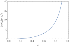
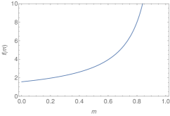
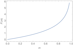
Figure 1: The quantities $\Delta(m)/(\sigma k_{0}^{2})$ (left), $f(m)$ (center) and $F(m)$ (right) as functions of $m$.

In closing, we return our attention to the eigenvalues $\lambda_{\pm}$ of the system, given by $\lambda_{\pm}=2\sigma q\pm\sqrt{\Delta(m)}$ [cf. (2.3)], where in light of (2.14), we can now express $\Delta$ as

$$\Delta(m)=16\sigma k_{0}^{2}K_{m}\frac{((1-m)K_{m}-2(2-m)E_{m}K_{m}+3E_{m}^{2})^{2}}{3E_{m}(K_{m}-E_{m})(E_{m}-(1-m)K_{m})}\,.$$ (2.1)

Note that $\Delta(m)/(\sigma k_{0}^{2})\to 0$ as $m\to 0$ and $\Delta(m)/(\sigma k_{0}^{2})\to+\infty$ as $m\to 1$ (cf. Fig. 1). When $m=0$, $\lambda_{\pm}=2\sigma q$ and $R_{\pm}=q$ so that (2.13) exhibits a one-component reduction in the harmonic limit to the inviscid Burgers equation. By monotonicity of $\Delta(m)$, the reduced $2\times 2$ system is strictly hyperbolic according to the following definition of strict hyperbolicity: $\lambda_{+}=\lambda_{-}$ if and only if $R_{+}=R_{-}$ [17]. It can also be shown that $({\kern-0.83337pt\lower 0.20004pt\hbox{$\nabla$}\kern-8.33336pt\lower 0.20004pt\hbox{\kern 0.50003pt\hbox{$\nabla$}}\kern-8.33336pt\raise 0.20004pt\hbox{$\nabla$}\kern-8.33336pt\raise 0.20004pt\hbox{\kern-0.50003pt\hbox{$\nabla$}}}_{m,q}\lambda_{\pm})\cdot{\mathbf{w}}_{\pm}\neq 0$, which implies that the system is genuinely nonlinear.

3 The XT system

Next we consider the reduction of the KPWS in which all fields are independent of $y$. Similarly to section 2, at first we consider the five-component original KPWS (1.1), ignoring the compatibility condition (1.0d). When solutions are independent of $y$, this system reduces to what we call the “XT system”, which in vector form is

$$I_{4}\frac{\partial{\mathbf{r}}}{\partial{t}}+A_{5}\frac{\partial{\mathbf{r}}}{\partial{x}}=0\,,$$ (3.1)

with ${\mathbf{r}}=(r_{1},r_{2},r_{3},q,p)^{T}$ as before, and $A_{5}$ given in (A.0f). We will obtain analogous results to section 2 even though the analysis of the systems and the physics they describe are significantly different.

3.1 Reduction to a four-component system, harmonic and soliton limits

In this case, reducing the size of the system is much easier than in section 2, because when all derivatives in $y$ vanish, the last equation in (3.1) determines $p$ in terms of $r_{1},r_{2},r_{3}$ by direct integration. Substituting the resulting expression into the PDEs for $r_{1},r_{2},r_{3}$ leads to the reduced system

$$\frac{\partial r_{j}}{\partial{t}}+(V_{j}-\sigma q^{2})\frac{\partial r_{j}}{\partial{x}}+\sigma q^{2}(1-\alpha)\frac{\partial r_{1}}{\partial{x}}+\sigma q^{2}\alpha\frac{\partial r_{3}}{\partial{x}}+\sigma q(\nu_{5}-\nu_{j})\frac{\partial q}{\partial{x}}=0\,,\quad j=1,2,3\,,$$

(3.0a)

$$\frac{\partial q}{\partial{t}}-q(4-\nu_{4})\frac{\partial r_{1}}{\partial{x}}+q(2+\nu_{4})\frac{\partial r_{3}}{\partial{x}}+(V_{2}-\sigma q^{2})\frac{\partial q}{\partial{x}}=0\,,$$ (3.0b)

or equivalently, in vector form,

$$\frac{\partial{\mathbf{r}}_{4}}{\partial{t}}+A_{4}\frac{\partial{\mathbf{r}}_{4}}{\partial{x}}=0\,,$$ (3.1)

where now ${\mathbf{r}}_{4}=(r_{1},r_{2},r_{3},q)^{T}$ and

$$A_{4}=\left(\begin{array}[]{cccc}V_{1}-\sigma q^{2}\alpha&0&\sigma q^{2}\alpha&\sigma q(\nu_{5}-\nu_{1})\\ \sigma q^{2}(1-\alpha)&V_{2}-\sigma q^{2}&\sigma q^{2}\alpha&\sigma q(\nu_{5}-\nu_{2})\\ \sigma q^{2}(1-\alpha)&0&V_{3}+\sigma q^{2}(\alpha-1)&\sigma q(\nu_{5}-\nu_{3})\\ -q(4-\nu_{4})&0&-q(2+\nu_{4})&V_{2}-\sigma q^{2}\end{array}\right)\,.$$ (3.2)

The above system simplifies considerably in the harmonic and soliton limits. The limiting values of all coefficients are found in the Appendix. In the harmonic limit, $m\to 0$, the PDEs for $r_{1}$ and $r_{2}$ coincide, and we can therefore choose the reduced set of dependent variables ${\mathbf{r}}_{3}=(r_{1},r_{3},q)^{T}$, obtaining

$$\frac{\partial{\mathbf{r}}_{3}}{\partial{t}}+A_{3}^{(0)}\frac{\partial{\mathbf{r}}_{3}}{\partial{x}}=0\,,$$ (3.3)

with

$$A_{3}^{(0)}=\left(\begin{array}[]{ccc}12r_{1}-6r_{3}-\sigma q^{2}&\sigma q^{2}&0\\ 0&6r_{3}&0\\ 0&6&12r_{1}-6r_{3}-\sigma q^{2}\end{array}\right)\,.$$ (3.4)

Equation (3.3) coincides with the $y$-independent reduction of the systems in [11], which were shown to be integrable. Conversely, in the soliton limit, $m\to 1$, the PDEs for $r_{2}$ and $r_{3}$ coincide. Choosing again ${\mathbf{r}}_{3}=(r_{1},r_{3},q)^{T}$, we obtain (3.3), but with $A_{3}^{(0)}$ replaced by

$$A_{3}^{(1)}=\left(\begin{array}[]{ccc}6r_{1}&0&0\\ \sigma q^{2}&2r_{1}+4r_{3}-\sigma q^{2}&\frac{4\sigma q}{3}(r_{1}-r_{3})\\ -2q&-4q&2r_{1}+4r_{3}-\sigma q^{2}\end{array}\right)\,.$$ (3.5)

This system also coincides with the $y$-independent reduction of the systems in [11], and is therefore integrable.

3.2 Riemann invariant, integrability, further reduction and diagonalization of the XT system

The matrix $A_{4}$ has the eigenvalue

$$\lambda_{o}=V_{2}-\sigma q^{2}\,,$$ (3.6)

with associated left eigenvector

$${\mathbf{w}}_{o}=\big{(}q(1-m)(K_{m}-E_{m})\,,\,q(E_{m}-(1-m)K_{m})\,,\,qmE_{m}\,,\,-2m(1-m)(r_{3}-r_{1})K_{m}\,\big{)}\,.$$

(3.7)

These expressions allow us to find a Riemann invariant and, in turn, to partially diagonalize the XT system (3.1). In this case however, the calculations are more complicated than those of section 2. We begin by applying ${\mathbf{w}}_{o}^{T}$ to (3.1), obtaining the characteristic relation

$$\frac{1}{(r_{3}-r_{1})K_{m}}\bigg{(}\frac{K_{m}-E_{m}}{m}{\rm d}r_{1}+\frac{E_{m}-(1-m)K_{m}}{(1-m)m}{\rm d}r_{2}-\frac{E_{m}}{1-m}{\rm d}r_{3}\bigg{)}-2\frac{{\rm d}q}{q}=0\,$$ (3.8)

along ${\rm d}{x}/{\rm d}{t}=V_{2}-\sigma q^{2}$ . To integrate this differential form and find the Riemann invariant, we first eliminate $r_{2}$ in favor of $m$ using (1.4), implying ${\rm d}r_{2}=(1-m)\,{\rm d}r_{1}+m\,{\rm d}r_{3}+(r_{3}-r_{1})\,{\rm d}m$, which yields

$$\frac{{\rm d}(r_{3}-r_{1})}{r_{3}-r_{1}}+\frac{E_{m}-(1-m)K_{m}}{m(1-m)K_{m}}\,{\rm d}m-2\frac{{\rm d}q}{q}=0\,.$$ (3.9)

Next, we eliminate $q$ in favor of $l$ using (1.1), implying ${\rm d}q={\rm d}l/k-l\,{\rm d}k/k^{2}$, and we use (1.0a) to replace $k$ and express ${\rm d}k={\rm d}(r_{3}-r_{1})/(4K_{m}\sqrt{r_{3}-r_{1}})-\sqrt{r_{3}-r_{1}}{\rm d}K_{m}/(2K_{m}^{2})$. Using equation (A.0a), substituting and simplifying, the resulting expression finally yields ${\rm d}l=0$. The Riemann invariant $R_{o}$ in this case is nothing else but the wavenumber in the $y$ direction, $R_{o}=l$, which satisfies the PDE

$$\frac{\partial R_{o}}{\partial{t}}+(V_{2}-\sigma q^{2})\frac{\partial R_{o}}{\partial{x}}=0\,.$$ (3.10)

The fact that $l$ is a Riemann invariant for the XT system is not an accident, and is related to its compatibility with the full KPWS and (as we will see below) with its integrability. This is because, when all fields are independent of $y$, the conservation of waves equations (1.2) yield $l_{x}=l_{t}=0$, implying that, for one-phase solutions of the KP equation, $l$ must be constant. We can use this relation to reduce the XT system (3.1) to a three-component system. To do this, we perform a change of dependent variable from ${\mathbf{r}}_{4}=(r_{1},r_{2},r_{3},q)^{T}$ to ${\mathbf{v}}=(r_{1},r_{2},r_{3},l)^{T}$, which results in the partially decoupled system

$${\mathbf{v}}_{t}+A_{4}^{\prime}\,{\mathbf{v}}_{x}=0\,,$$ (3.11)

with

$$A_{4}^{\prime}=\left(\begin{array}[]{cc}A_{3}&{\mathbf{a}}_{3}\\ {\mathbf{0}}_{3}^{T}&V_{2}-\sigma q^{2}\end{array}\right)\,,\qquad$$ (3.12)

where the three-component vector ${\mathbf{a}}_{3}$ is immaterial for our purposes, ${\mathbf{0}}_{3}=(0,0,0)^{T}$ and

$$A_{3}=A_{\mathrm{KdV}}+\frac{4\sigma K_{m}l^{2}}{3(r_{2}-r_{1})}A_{3}^{(2)}\,,$$ (3.0a)

$$A_{\mathrm{KdV}}=\mathop{\rm diag}\nolimits(V_{1},V_{2},V_{3})\,,$$ (3.0b)

$$A_{3}^{(2)}=\left(\begin{array}[]{ccc}2a_{3}&\frac{a_{1}a_{4}}{(1-m)(K_{m}-E_{m})}&\frac{mE_{m}a_{2}}{(1-m)(K_{m}-E_{m})}\\[1.72218pt] \frac{-(K_{m}-E_{m})a_{4}}{a_{1}}&-\frac{2a_{2}}{1-m}&-\frac{E_{m}ma_{3}}{(1-m)a_{1}}\\[1.72218pt] \frac{(K_{m}-E_{m})a_{2}}{E_{m}}&\frac{a_{1}a_{3}}{(1-m)E_{m}}&-\frac{2ma_{4}}{1-m}\end{array}\right)\,,$$ (3.0f)

with $V_{1},\dots,V_{3}$ as in (1) and

$$a_{1}=E_{m}-(1-m)K_{m}\,,\quad a_{2}=(1-m)K_{m}+(2m-1)E_{m}\,,$$ (3.0g)

$$a_{3}=(1-m)K_{m}-(1+m)E_{m}\,,\quad a_{4}=2(1-m)K_{m}-(2-m)E_{m}\,.$$ (3.0h)

Since $l$ is constant for compatible solutions of the full KPWS, we can solve the fourth equation in (3.11) by taking $l\equiv l_{0}$, thereby arriving at a three-component system of the same form as (3.3)

$$\frac{\partial{\mathbf{r}}_{3}}{\partial{t}}+A_{3}\,\frac{\partial{\mathbf{r}}_{3}}{\partial{x}}=0\,,$$ (3.1)

except that now ${\mathbf{r}}_{3}=(r_{1},r_{2},r_{3})^{T}$ and the coefficient matrix $A_{3}$ is given by (3.12). The case $l_{0}=0$ yields $A_{3}=A_{\mathrm{KdV}}$, so the system (3.1) reduces exactly to the KdV-Whitham system of Whitham modulation equations for the KdV equation [35]. We have therefore showed that, once compatibility is enforced, the XT system reduces to a one-parameter deformation of the KdV-Whitham system, parametrized by the value of the wavenumber $l_{0}$ along the transverse dimension.

We now turn to the issue of the integrability of the XT system. We apply the Haantjes tensor test to the four-component XT system (3.1) and find that it fails. At the same time, the harmonic and soliton limits of the XT system discussed earlier are clearly integrable, since they are exact one-dimensional reductions of the the harmonic and soliton limits of the full KPWS, which were shown to be integrable in [11]. On the other hand, the three-component reduced system (3.1) does pass the Haantjes test, in that all the terms of its Haantjes tensor associated with $A_{3}$ in (3.12) vanish identically. Thus, while the system (3.1) is not integrable, the system (3.1) is an integrable, one-parameter family of deformations of the KdV-Whitham system.

The harmonic limit (i.e., $r_{2}\to r_{1}$, implying $m\to 0$) of the deformed three-component system (3.1) yields the coefficient matrix

$$\lim_{r_{2}\to r_{1}}A_{3}=\left(\begin{array}[]{ccc}12r_{1}-6r_{3}-\sigma q^{2}&0&\sigma q^{2}\\ 0&12r_{1}-6r_{3}-\sigma q^{2}&\sigma q^{2}\\ 0&0&6r_{3}\end{array}\right)$$ (3.2)

with $q^{2}=\pi^{2}l_{0}^{2}/(r_{3}-r_{1})$, which is consistent with the system (3.3). On the other hand, like with the reduced YT system, the soliton limit (i.e., $r_{2}\to r_{3}$, implying $m\to 1$) of the reduced XT system (3.1) is singular for $l_{0}\neq 0$, since some of the entries of $A_{3}^{(2)}$ diverge in that limit. Again, this is to be expected, because in the soliton limit one has $l_{0}=0$ [cf. (1.0a)].

3.3 Deformed Riemann invariants

Since the one-parameter deformation (3.1) of the KdV-Whitham system is integrable, it can be written in diagonal form. We have not been able to determine the deformed Riemann invariants for all parameter values $l$ but we can obtain approximate Riemann invariants for small $l$ following standard methodology (e.g., see [20]). It is convenient to define the coefficient

$$c_{2}=\frac{4K_{m}}{3m(r_{2}-r_{1})}\,,$$ (3.3)

so that (3.12) reads $A_{3}=A_{\mathrm{KdV}}+A_{\mathrm{def}}$ and the “deformation matrix” is simply $A_{\mathrm{def}}=\ell c_{2}A_{3}^{(2)}$ with the (signed) deformation parameter

$$\ell\equiv\sigma l_{0}^{2}.$$ (3.4)

We seek an expansion of the deformed eigenvalues ${\tilde{V}}_{j}$ and corresponding right eigenvectors ${\tilde{\mathbf{v}}}_{j}$ in powers of $\ell$ as

$${\tilde{V}}_{j} =V_{j}+\ell V_{j}^{(2)}({\mathbf{r}}_{3})+O(\ell^{2}),\qquad{\tilde{\mathbf{v}}}_{j} ={\mathbf{e}}_{j}+\ell{\mathbf{v}}_{j}^{(2)}({\mathbf{r}}_{3})+O(\ell^{2}),\qquad j=1,2,3,$$ (3.5)

where ${\mathbf{r}}_{3}=(r_{1},r_{2},r_{3})^{T}$ are the unperturbed KdV-Whitham Riemann invariants, the unperturbed speeds $V_{j}$ are given in (1), and the unperturbed eigenvectors ${\mathbf{e}}_{1},{\mathbf{e}}_{2},{\mathbf{e}}_{3}$ are simply the canonical basis in ${\mathbb{R}}^{3}$, i.e., $({\mathbf{e}}_{1},{\mathbf{e}}_{2},{\mathbf{e}}_{3})={\mathbb{I}}_{3}$, where ${\mathbb{I}}_{n}$ is the $n\times n$ identity matrix. We begin by computing the perturbation to the characteristic speeds. Since $A_{\mathrm{def}}=O(\ell)$, the first correction terms appear at $O(\ell)$. The deformed eigenvalue problem is

$$(A_{\mathrm{KdV}}+A_{\mathrm{def}})\,{\tilde{\mathbf{v}}}_{j}={\tilde{V}}_{j}{\tilde{\mathbf{v}}}_{j}\,,\qquad j=1,2,3.$$ (3.6)

The unperturbed eigenvalue problem, obtained at $O(1)$, is simply $A_{\mathrm{KdV}}{\mathbf{e}}_{i}=V_{i}{\mathbf{e}}_{i}$, which is satisfied because the KdV-Whitham system is the $\ell=0=l_{0}$ reduction of the XT system (3.1). Collecting terms $O(\ell)$ in (3.6) yields

$$(A_{\mathrm{KdV}}-V_{j}{\mathbb{I}}_{3}){\mathbf{v}}_{j}^{(2)}=(V_{j}^{(2)}-c_{2}A_{3}^{(2)}){\mathbf{e}}_{j}\,,$$ (3.7)

and multiplying from the left by ${\mathbf{e}}_{j}^{T}$ yields the first-order correction to the characteristic velocities as

$$V_{j}^{(2)}={\mathbf{e}}_{j}^{T}c_{2}A_{3}^{(2)}{\mathbf{e}}_{j}\,,\qquad j=1,2,3\,,$$ (3.8)

since the ${\mathbf{e}}_{j}$ are orthonormal. Explicitly,

$${\tilde{V}}_{1}=V_{1}^{(0)}-2c_{2}\ell\left((1+m)E_{m}-(1-m)K_{m}\right)+O(\ell^{2}),$$ (3.0a)

$${\tilde{V}}_{2}=V_{2}^{(0)}-2c_{2}\ell\frac{(1-m)K_{m}-(1-2m)E_{m}}{1-m}+O(\ell^{2}),$$ (3.0b)

$${\tilde{V}}_{3}=V_{3}^{(0)}+2c_{2}\ell m\frac{(2-m)E_{m}-2(1-m)K_{m}}{1-m}+O(\ell^{2})\,.$$ (3.0c)

Note that if $\sigma=1$, the corrections to the first and second characteristic velocities are negative, while the correction to the third characteristic velocity is positive (opposite if $\sigma=-1$). Note also that all three corrections remain finite in the limit $m\to 0$, but diverge as $m\to 1$, indicating that the harmonic limit of the deformed system is finite, but its soliton limit is singular for $\ell\neq 0$. This is expected because the soliton limit requires $l_{0}=0$, which is only true when the XT system (3.1) reduces to the KdV-Whitham system. Next, we use (3.7) and (3.8) to compute the correction to the eigenvectors. The matrix $A_{\mathrm{KdV}}-V_{j}{\mathbb{I}}_{3}$ is singular for $j=1,2,3$. Nonetheless, the inhomogeneous linear system admits a solution, which yields the deformed eigenvectors in the form

$${\mathbf{{\tilde{v}}_{1}}}=\left(\!\!\begin{array}[]{c}1\\ 0\\ 0\end{array}\!\!\right)+c_{2}\ell\left(\!\!\begin{array}[]{c}0\\ 1\\ m\end{array}\!\!\right),\quad{\mathbf{{\tilde{v}}_{2}}}=\left(\!\!\begin{array}[]{c}0\\ 1\\ 0\end{array}\!\!\right)+c_{2}\ell\left(\!\!\begin{array}[]{c}m-1\\ 0\\ m\end{array}\!\!\right),\quad{\mathbf{{\tilde{v}}_{3}}}=\left(\!\!\begin{array}[]{c}0\\ 0\\ 1\end{array}\!\!\right)+c_{2}\ell\left(\!\!\begin{array}[]{c}m-1\\ 1\\ 0\end{array}\!\!\right),$$ (3.19)

up to $O(\ell^{2})$ terms.

Next we compute the deformed Riemann invariants. It is non-trivial to find the correct integrating factor for the deformed Riemann invariants. To circumvent this issue, we take advantage of the fact that the total differential of each Riemann invariant is zero along the associated characteristic curve. We expand the deformed Riemann invariants ${\tilde{R}}_{1},{\tilde{R}}_{2},{\tilde{R}}_{3}$ as

$${\tilde{R}}_{j}=r_{j}+\ell R^{(2)}_{j}({\mathbf{r}}_{3})+O(\ell^{2})\,,\qquad j=1,2,3\,.$$ (3.21)

We have

$${\rm d}{\tilde{R}}_{j}=0$$ (3.22)

along the characteristic curve ${\rm d}x/{\rm d}t={\tilde{V}}_{j}$, for $j=1,2,3$. Expanding (3.22) yields

$${\rm d}{\tilde{R}}_{j}={\kern-0.83337pt\lower 0.20004pt\hbox{$\nabla$}\kern-8.33336pt\lower 0.20004pt\hbox{\kern 0.50003pt\hbox{$\nabla$}}\kern-8.33336pt\raise 0.20004pt\hbox{$\nabla$}\kern-8.33336pt\raise 0.20004pt\hbox{\kern-0.50003pt\hbox{$\nabla$}}}_{{\mathbf{r}}}{\tilde{R}}_{j}\cdot{\rm d}{\mathbf{r}}={\kern-0.83337pt\lower 0.20004pt\hbox{$\nabla$}\kern-8.33336pt\lower 0.20004pt\hbox{\kern 0.50003pt\hbox{$\nabla$}}\kern-8.33336pt\raise 0.20004pt\hbox{$\nabla$}\kern-8.33336pt\raise 0.20004pt\hbox{\kern-0.50003pt\hbox{$\nabla$}}}_{{\mathbf{r}}}{\tilde{R}}_{j}\cdot\bigg{(}\frac{\partial{\mathbf{r}}_{3}}{\partial{t}}{\rm d}t+\frac{\partial{\mathbf{r}}_{3}}{\partial{x}}{\rm d}x\bigg{)}=0\,,\qquad j=1,2,3\,,$$ (3.23)

where ${\kern-0.83337pt\lower 0.20004pt\hbox{$\nabla$}\kern-8.33336pt\lower 0.20004pt\hbox{\kern 0.50003pt\hbox{$\nabla$}}\kern-8.33336pt\raise 0.20004pt\hbox{$\nabla$}\kern-8.33336pt\raise 0.20004pt\hbox{\kern-0.50003pt\hbox{$\nabla$}}}_{{\mathbf{r}}}=(\partial_{r_{1}},\partial_{r_{2}},\partial_{r_{3}})^{T}$. Next we use (3.1) and (3.6) to rewrite (3.23) as

$$({\kern-0.83337pt\lower 0.20004pt\hbox{$\nabla$}\kern-8.33336pt\lower 0.20004pt\hbox{\kern 0.50003pt\hbox{$\nabla$}}\kern-8.33336pt\raise 0.20004pt\hbox{$\nabla$}\kern-8.33336pt\raise 0.20004pt\hbox{\kern-0.50003pt\hbox{$\nabla$}}}_{{\mathbf{r}}}{\tilde{R}}_{j})^{T}({\tilde{V}}_{j}{\mathbb{I}}_{3}-A_{3})\frac{\partial{\mathbf{r}}_{3}}{\partial x}\,{\rm d}t=0\,,\qquad j=1,2,3\,,$$ (3.24)

along the curve ${\rm d}x/{\rm d}t={\tilde{V}}_{j}$. If the above differential must be zero for all $\frac{\partial{\mathbf{r}}_{3}}{\partial x}$, one can constrain each component to be zero, i.e.,

$$({\kern-0.83337pt\lower 0.20004pt\hbox{$\nabla$}\kern-8.33336pt\lower 0.20004pt\hbox{\kern 0.50003pt\hbox{$\nabla$}}\kern-8.33336pt\raise 0.20004pt\hbox{$\nabla$}\kern-8.33336pt\raise 0.20004pt\hbox{\kern-0.50003pt\hbox{$\nabla$}}}_{{\mathbf{r}}}{\tilde{R}}_{j})^{T}({\tilde{V}}_{j}{\mathbb{I}}_{3}-A_{3})={\mathbf{0}}\,,\qquad j=1,2,3\,.$$ (3.25)

One can check that $\det({\tilde{V}}_{j}{\mathbb{I}}_{3}-A_{3})=O(\ell^{2})$ for $j=1,2,3$, which allows for a nontrivial solution at $O(\ell)$. For each $j=1,2,3$, (3.25) yields a system of three differential equations for $R^{(2)}_{j}$. Note that, even though it might not seem obvious a priori, these differential equations must necessarily be compatible since we know that the system is integrable and therefore admits Riemann invariants.

We present the calculations for $R^{(2)}_{1}$ in detail. Keeping terms up to $O(\ell)$, the first equation in (3.25) is trivially satisfied, while the remaining two equations are

$$\frac{\partial R^{(2)}_{1}}{\partial{r_{2}}} =\frac{(E_{m}-(1-m)K_{m})^{2}}{3(1-m)(r_{2}-r_{1})^{2}}\,,$$ (3.0a)

$$\frac{\partial R^{(2)}_{1}}{\partial{r_{3}}} =-\frac{m^{2}E_{m}^{2}}{3(1-m)(r_{2}-r_{1})^{2}}\,,$$ (3.0b)

and one can check that the equality of the mixed second derivatives, namely $\partial^{2}R^{(2)}_{1}/\partial{r_{2}}\partial{r_{3}}=\partial^{2}{R^{(2)}_{1}}\partial{r_{3}}\partial{r_{2}}$, is indeed satisfied. Next, we need to integrate (3.3) to find $R^{(2)}_{1}$. We can integrate the equations manually, employing a process akin to that of finding a potential for a conservative vector field. We begin with (3.0b) since it is simpler. Because of the presence of elliptic integrals, it is convenient to perform a change of variables from $r_{1},r_{2},r_{3}$ to $r_{1},r_{2}$ and $m$. Solving (1.4) for $r_{3}$ as a function of $m$, we have

$$\frac{\partial R^{(2)}_{1}}{\partial{m}}=\frac{\partial R^{(2)}_{1}}{\partial{r_{3}}}\frac{\partial r_{3}}{\partial{m}}=\frac{E_{m}^{2}}{3(1-m)(r_{2}-r_{1})}\,.$$ (3.1)

Integrating this equation (with $r_{1}$ and $r_{2}$ held constant) then yields $R^{(2)}_{1}$ as

$$R^{(2)}_{1}=\frac{g(m)}{3(r_{2}-r_{1})}\,,$$ (3.0a)

$$g^{\prime}(m)=\frac{E_{m}^{2}}{1-m}\,.$$ (3.0b)

Note that we have taken the arbitrary function of $r_{1}$ and $r_{2}$ in (3.0a) to be zero. By substituting (3.0a) into (3.0a) yields

$$g(m)=-(1-m)K_{m}^{2}+2E_{m}K_{m}-E_{m}^{2}\,,$$ (3.0c)

and one can confirm that (3.0c) is indeed compatible with (3.0b), which means we have successfully integrated (3.3), obtaining the first approximate deformed Riemann invariant of the XT system as

$${\tilde{R}}_{1}=r_{1}+\frac{\ell}{3(r_{2}-r_{1})}(2K_{m}E_{m}-E_{m}^{2}-(1-m)K_{m}^{2})+O(\ell^{2})\,.$$ (3.0a)

One can apply an identical process to find the remaining deformed Riemann invariants as

$${\tilde{R}}_{2}=r_{2}+\frac{\ell}{4K_{m}}\bigg{(}2K_{m}E_{m}+\frac{E_{m}^{2}}{1-m}-(1-m)K_{m}^{2}\bigg{)}+O(\ell^{2})\,,$$ (3.0b)

$${\tilde{R}}_{3}=r_{3}-\frac{\ell}{3(r_{2}-r_{1})}\frac{m((1-m)K_{m}^{2}-E_{m}^{2})}{1-m}+O(\ell^{2})\,.$$ (3.0c)

The expressions of the deformed speeds and deformed Riemann invariants may prove to be useful when investigating the dynamics of weakly slanted wave fronts in the KP equation.

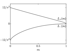
Figure 2: The functions $L_{\pm}(m)$ that determine the critical values $m=m_{\pm}$ at which two characteristic velocities of the XT system coalesce.

3.4 Hyperbolicity

The hyperbolicity of the three-component reduction (3.1) of the full KPWS can be determined by analyzing the eigenvalues of the coefficient matrix $A_{3}({\mathbf{r}}_{3})$, given in (3.12), which are the characteristic velocities $\tilde{V}_{j}$, $j=1,2,3$. Because the characteristic polynomial

$$p(\lambda)=\det(A_{3}-\lambda{\mathbb{I}}_{3})=-\lambda^{3}+b_{2}\lambda^{2}+b_{1}\lambda+b_{0},$$ (3.1)

is a cubic with real coefficients, it has either three real roots or one real root and a complex conjugate pair. Equation (3.8) demonstrates that the $\tilde{V}_{j}$ are real for all $r_{j}\in{\mathbb{R}}$ with $r_{1}\leq r_{2}\leq r_{3}$ when the deformation parameter $\ell=\sigma l_{0}^{2}$ is sufficiently small in magnitude. Because the coefficients $b_{0},b_{1},b_{2}$ in (3.1) are smooth functions of ${\mathbf{r}}_{3}$, a bifurcation from all real roots to a complex conjugate pair can only occur if the discriminant of $p(\lambda)$,

$$D({\mathbf{r}}_{3})=4b_{1}^{3}+b_{2}^{2}b_{1}^{2}-18b_{0}b_{2}b_{1}-4b_{0}b_{2}^{3}-27b_{0}^{2}\,,$$ (3.2)

is zero. To evaluate $D({\mathbf{r}}_{3})$, we first simplify the calculation by restricting ourselves to the set

$$S=\left\{{\mathbf{r}}_{3}=(0,m,1)^{T}~{}|~{}0\leq m\leq 1\right\}\,,$$ (3.3)

and we simply write $D=D(m)$, which can be shown to be a quintic polynomial in $\ell$ with coefficients depending on $m$. Setting $D(m)=0$ and solving for $\ell$, one finds two complex conjugate solutions, which are not of interest, plus two real solutions $\ell=L_{-}(m)$ and $\ell=L_{+}(m)$, the latter of which is a double root. Explicitly,

$$L_{+}(m)=\frac{((2-m)E_{m}-2(1-m)K_{m})((1+m)E_{m}-(1-m)K_{m})((1-m)K_{m}-(1-2m)E_{m})}{3E_{m}(K_{m}-E_{m})(E_{m}-(1-m)K_{m})\left(2(2-m)K_{m}E_{m}-3E_{m}^{2}-(1-m)K_{m}^{2}\right)},$$

while the expression for $L_{-}(m)$ is more complicated, so it is omitted for brevity. The expansions of $L_{\pm}(m)$ for small $m$ are

$$L_{+}(m) =\frac{12}{\pi^{2}}(1-m)+O(m^{2}),$$ (3.5)

$$L_{-}(m) =-\frac{12}{\pi^{2}}\left(1-\frac{4}{3}(2m)^{2/3}-m\right)+O(m^{4/3}).$$ (3.6)

Figure 2 shows that $L_{+}(m)>0$ and $L_{-}(m)<0$ for $m\in[0,1)$. Therefore, there are two critical values of $m$: $\ell=\pm l_{0}^{2}=L_{\pm}(m_{\pm})$. The fact that $\tilde{V}_{j}\in{\mathbb{R}}$ for $|\ell|$ sufficiently small implies that $D(m)>0$ when $0<m<m_{\pm}$, namely the XT system is (strictly) hyperbolic when $m\in(0,m_{\pm})$. When $m=m_{\pm}$, two characteristic velocities coalesce.

In the case of the plus sign, the fact that $\ell=L_{+}(m_{+})$ is a double root of $D(m)=0$ implies that ${\rm d}D/{\rm d}m\,|_{m_{+}}=0$. Then, in a neighborhood of $m=m_{+}$, the discriminant (3.2) exhibits parabolic behavior

$$D(m)=\frac{1}{2}\left.\frac{\mathrm{d}^{2}D}{\mathrm{d}m^{2}}\right|_{m_{+}}(m-m_{+})^{2}+O(m-m_{+})^{3}\,,$$ (3.7)

and it must be the case that $D(m)\geq 0$, i.e., ${\rm d}^{2}D/{\rm d}m^{2}|_{m_{+}}>0$, because $D(m)>0$ for $0<m<m_{+}$. Since $m_{+}$ is the only point at which $D(m)=0$, this implies $D(m)>0$ for $m\in[0,m_{+})\cup(m_{+},1)$ and that the characteristic speeds are always real. Indeed, a direct calculation shows that, when $m=m_{+}$,

$$\tilde{V}_{1} =\tilde{V}_{2}=\frac{6\left((1+m)E(m)^{2}-(1-m)^{2}K(m)^{2}-2(1-m)mK(m)E(m)\right)}{(1-m)K(m)^{2}-2(2-m)K(m)E(m)+3E(m)^{2}},$$ (3.0a)

$$\tilde{V}_{3} =\frac{2}{3}\left(3(m+1)+\frac{2mE(m)}{(m-1)K(m)+E(m)}+\frac{2mE(m)}{K(m)-E(m)}-\frac{2(1-m)K(m)}{E(m)}\right)$$ (3.0b)

and there are three corresponding linearly independent eigenvectors ${\bf\tilde{v}_{j}}$, $j=1,2,3$. Consequently, we conclude that the XT system is hyperbolic for $m\in(0,1)$ and strictly hyperbolic when $m\neq m_{+}$.

In the case of the minus sign, the critical point $m_{-}$ satisfying $\ell=-l_{0}^{2}=L_{-}(m_{-})$ is a simple root of $D(m)$. Since $D(m)>0$ for $0<m<m_{-}$ and $D$ depends upon $m$ smoothly, it necessarily is the case that ${\rm d}D/{\rm d}m\,|_{m_{-}}<0$, so that the discriminant (3.2) becomes negative in a right neigborhood of $m=m_{-}$. This implies that, for $m_{-}<m<1$, the XT system exhibits a complex conjugate pair of characteristic speeds and is not hyperbolic.

The above discussion of hyperbolicity of the XT system was limited to the set $S$ defined in (3.3), where it was observed that a bifurcation occurs at the point $m=m_{\sigma}$. However, using the scaling symmetry $r_{j}(x,t)\to a^{2}r_{j}(ax,a^{3}t)$, $q(x,t)\to aq(ax,a^{3}t)$ with $a=(r_{3}-r_{1})^{-1/2}$ and the Galilean symmetry $r_{j}(x,t)\to b+r_{j}(x-6bt,t)$, $q(x,t)\to q(x-6bt,t)$ with $b=-r_{1}$ [4], we can map any vector ${\mathbf{r}}_{3}=(r_{1},r_{2},r_{3})^{T}\in{\mathbb{R}}^{3}$ with $r_{1}\leq r_{2}\leq r_{3}$ to a vector ${\tilde{\mathbf{r}}_{3}}=(0,m,1)^{T}\in S$. For ${\mathbf{r}}_{3}$, the bifurcation occurs on the surface

$$\Sigma_{\pm}=\left\{{\mathbf{r}}_{3}=(r_{1},r_{2},r_{3})^{T}~{}\Big{|}~{}\pm l_{0}^{2}=L_{\pm}(m_{\pm})(r_{3}-r_{1})^{2},~{}~{}m_{\pm}=\frac{r_{2}-r_{1}}{r_{3}-r_{1}}\right\}.$$ (3.1)

In the case of the plus sign, the XT system is hyperbolic, and strictly so for ${\mathbf{r}}_{3}\notin\Sigma_{+}$. In the case of the minus sign, the XT system is hyperbolic so long as $(r_{2}-r_{1})/(r_{3}-r_{1})<m_{-}$ where, $L_{-}(m_{-})=-l_{0}^{2}(r_{3}-r_{1})^{2}$. When $(r_{2}-r_{1})/(r_{3}-r_{1})>m_{-}$, the XT system loses hyperbolicity.

4 The XY system

4.1 KPWS in a comoving frame and the XY system

The third and final class of reductions of the KPWS we consider is that of time-independent solutions, to be defined precisely below. While in Sections 2 and 3 we considered reductions that are evolutionary, exhibiting well-posed initial value problems (at least when $\sigma=1$), here we are considering a spatial problem, independent of $t$, for the modulations. As we will see, this does not preclude dynamics in the full solution to KP itself. In the previous sections we saw that, in order to ensure the compatibility of the XT and YT reductions with the KP equation, one must make sure that all three conservation of waves equations (1.2) are satisfied. We will see that this is also the case with stationary reductions of the KPWS.

Note that, even though one may think that a more general scenario is obtained by looking for traveling wave solutions, i.e., solutions that are stationary in a traveling frame of reference $({\tilde{x}},{\tilde{y}},{\tilde{t}})$, with ${\tilde{x}}=x-ct$, ${\tilde{y}}=y-dt$ and ${\tilde{t}}=t$, this is not the case in practice. This is because the Galilean and pseudo-rotation invariance of the KP equation allow one to perform appropriate transformations of the dependent and independent variables to rewrite any traveling wave solution of the KP equation as stationary in a suitable reference frame. Since the KPWS preserves these invariances, the same transformations will also work for the KPWS, see Appendix A.2 for details.

Based on the above discussion, consider situations in which the temporal derivatives in the original KPWS (1.1) can be neglected, which then yields

$$A_{5}\,\frac{\partial{\mathbf{r}}}{\partial{x}}+B_{5}\,\frac{\partial{\mathbf{r}}}{\partial{y}}=0\,.$$ (4.1)

Contrary to the reductions discussed in 2 and 3, here the independence from one of the coordinates does not automatically result in a reduction in the number of degrees of freedom. That is, all five dependent variables appear in (4.1). Assuming invertibility of $A_{5}$ and $B_{5}$, one could equivalently write (4.1) as an evolutionary system with respect to either $x$ or $y$, e.g., as ${\mathbf{r}}_{x}+C\,{\mathbf{r}}_{y}=0$. However, the resulting coefficient matrix $C=(A_{5})^{-1}B_{5}$ is quite complicated, and therefore the resulting system is difficult to analyze.

4.2 Harmonic and soliton limits of the XY system

Similar to the XT and YT systems, the XY system admits finite harmonic and soliton limits, in which case the system simplifies considerably. Specifically, in the harmonic limit ($r_{2}\to r_{1}^{+}$, corresponding to $m\to 0$), the PDEs for $r_{1}$ and $r_{2}$ coincide, and (4.1) reduces to a four-component system of PDEs for the vector ${\mathbf{r}}^{\prime}=(r_{1},r_{3},q,p)^{T}$, in which the coefficient matrices $A_{5}$ and $B_{5}$ are replaced by

$$A_{4,o}=\left(\begin{array}[]{ccccc}12r_{1}-6r_{3}-\sigma q^{2}&0&-qr_{3}\sigma&-q\sigma\\ 0&6r_{3}-\sigma q^{2}&-qr_{3}\sigma&-q\sigma\\ 0&-6q&12r_{1}-6r_{3}-\sigma q^{2}&0\\ 0&q&r_{3}&1\end{array}\right),$$ (4.0e)

$$B_{4,o}=\left(\begin{array}[]{ccccc}2q\sigma&0&r_{3}\sigma&\sigma\\ 0&2q\sigma&r_{3}\sigma&\sigma\\ 0&6&2\sigma q&0\\ 0&-1&0&0\end{array}\right).$$ (4.0j)

Similarly, in the soliton limit ($r_{2}\to r_{3}^{-}$, corresponding to $m\to 1$), the PDEs for $r_{2}$ and $r_{3}$ coincide, and one obtains a four-component system for ${\mathbf{r}}^{\prime}=(r_{1},r_{3},q,p)^{T}$, with the matrices $A_{5}^{\prime}$ and $B_{5}^{\prime}$ replaced by

$$A_{4,1}=\left(\begin{array}[]{ccccc}6r_{1}-\sigma q^{2}&0&-qr_{1}\sigma&-q\sigma\\ 0&2r_{1}+4r_{3}-\sigma q^{2}&\frac{1}{3}q\sigma(r_{1}-4r_{3})&-q\sigma\\ -2q&-4q&2r_{1}+4r_{3}-\sigma q^{2}&0\\ q&0&r_{1}&1\end{array}\right),$$ (4.0e)

$$B_{4,1}=\left(\begin{array}[]{ccccc}2q\sigma&0&r_{1}\sigma&\sigma\\ 0&2q\sigma&-\frac{1}{3}\sigma(r_{1}-4r_{3})&\sigma\\ 2&4&2\sigma q&0\\ -1&0&0&0\end{array}\right).$$ (4.0j)

These systems coincide with the time-independent reduction of the harmonic and soliton limits studied in [4, 11], where it was also shown that these systems are integrable.

4.3 Riemann invariant, reduction and integrability

In light of what we learned by studying the YT and XT systems, we expect that, when considering solutions that are independent of $t$, the frequency $\omega$ will be one of the Riemann invariants. Indeed, in this case the three compatibility conditions (1.2) yield immediately $\omega_{x}=\omega_{y}=0$. We now show that this expectation is correct. In this case, however, the complexity of the system makes it impractical to use the direct approach based on the use of the characteristic relations and left eigenvectors that was used in the previous sections. We therefore use an alternative approach, based on calculating the total differential of $\omega=\omega(\mathbf{r})$ as

$${\rm d}\omega={\kern-0.83337pt\lower 0.20004pt\hbox{$\nabla$}\kern-8.33336pt\lower 0.20004pt\hbox{\kern 0.50003pt\hbox{$\nabla$}}\kern-8.33336pt\raise 0.20004pt\hbox{$\nabla$}\kern-8.33336pt\raise 0.20004pt\hbox{\kern-0.50003pt\hbox{$\nabla$}}}_{{\mathbf{r}}}\omega\cdot{\rm d}{\mathbf{r}}={\kern-0.83337pt\lower 0.20004pt\hbox{$\nabla$}\kern-8.33336pt\lower 0.20004pt\hbox{\kern 0.50003pt\hbox{$\nabla$}}\kern-8.33336pt\raise 0.20004pt\hbox{$\nabla$}\kern-8.33336pt\raise 0.20004pt\hbox{\kern-0.50003pt\hbox{$\nabla$}}}_{{\mathbf{r}}}\omega\cdot\bigg{(}\frac{\partial{\mathbf{r}}}{\partial{x}}{\rm d}x+\frac{\partial{\mathbf{r}}}{\partial{y}}{\rm d}y\bigg{)}\,,$$ (4.0a)

with ${\kern-0.83337pt\lower 0.20004pt\hbox{$\nabla$}\kern-8.33336pt\lower 0.20004pt\hbox{\kern 0.50003pt\hbox{$\nabla$}}\kern-8.33336pt\raise 0.20004pt\hbox{$\nabla$}\kern-8.33336pt\raise 0.20004pt\hbox{\kern-0.50003pt\hbox{$\nabla$}}}_{{\mathbf{r}}}=(\partial_{r_{1}},\partial_{r_{2}},\partial_{r_{3}},\partial_{q},\partial_{p})^{T}$. The evolution of $\omega$ as dictated by the system (4.1) along the characteristic coordinates $dy/dx=\lambda$ is then

$${\rm d}\omega={\kern-0.83337pt\lower 0.20004pt\hbox{$\nabla$}\kern-8.33336pt\lower 0.20004pt\hbox{\kern 0.50003pt\hbox{$\nabla$}}\kern-8.33336pt\raise 0.20004pt\hbox{$\nabla$}\kern-8.33336pt\raise 0.20004pt\hbox{\kern-0.50003pt\hbox{$\nabla$}}}_{{\mathbf{r}}}\omega\cdot\big{(}\lambda{\mathbb{I}}_{5}-C\big{)}\,\frac{\partial{\mathbf{r}}}{\partial{y}}\,{\rm d}x\,,$$ (4.0b)

with $C=(A_{5})^{-1}B_{5}$. Computing ${\kern-0.83337pt\lower 0.20004pt\hbox{$\nabla$}\kern-8.33336pt\lower 0.20004pt\hbox{\kern 0.50003pt\hbox{$\nabla$}}\kern-8.33336pt\raise 0.20004pt\hbox{$\nabla$}\kern-8.33336pt\raise 0.20004pt\hbox{\kern-0.50003pt\hbox{$\nabla$}}}_{{\mathbf{r}}}\omega$, substituting in (4.0b) and setting ${\rm d}\omega=0$ then yields a linear equation that determines the characteristic speed $\lambda$ as

$$\lambda=\frac{2\sigma q}{V_{2}-\sigma q^{2}},$$ (4.1)

with $V_{2}$ given in (1), which confirms that $\omega$ is indeed a Riemann invariant for the system (4.1).

As per the above discussion, in order for the KPWS to be compatible, we must enforce $\omega_{x}=\omega_{y}=0$. Following the procedures of section 2 and 3, we partially diagonalize the $XY$ system (4.1) by performing a dependent coordinate transformation so that $\omega$ is one of the new dependent variables. We then solve the resulting PDE by taking $\omega\equiv{}$const and obtain a one-parameter family of reduced four-component systems, parametrized by the constant value of $\omega$. Once again, however, the calculations are more involved than in the previous cases.

The complication is that the expression (1.1) for $\omega$ does not allow one to uniquely obtain any one of the dependent variables in terms of the others (recall (1.0a)). The best one can do is to solve for $q$, which entails a choice of sign:

$$q=\pm\sqrt{\sigma\bigg{(}\frac{\omega}{k}-V\bigg{)}}\,.$$ (4.2)

Following the same methods as in the previous sections, one can then obtain a four-component hydrodynamic system of equations for ${\mathbf{v}}=(r_{1},r_{2},r_{3},p)^{T}$. A single coefficient matrix of the form

$$\frac{\partial{\mathbf{v}}}{\partial{x}}+C_{4}^{\prime}\,\frac{\partial{\mathbf{v}}}{\partial{y}}=0\,,$$ (4.3)

is quite complicated. However, the system (4.1) can be transformed, using the same methods, into the concise form

$$A^{\prime}\frac{\partial{\mathbf{u}}}{\partial{x}}+B^{\prime}\frac{\partial{\mathbf{u}}}{\partial{y}}=0\,,$$ (4.4)

where $A^{\prime}=AT$ and $B^{\prime}=BT$ and ${\mathbf{u}}=(r_{1},r_{2},r_{3},\omega,p)^{T}$. Once the PDE for $\omega$ is disregarded, since $\omega\equiv{}$const solves it, we arrive at the system

$$A_{4}^{\prime}\frac{\partial{\mathbf{p}}}{\partial{x}}+B_{4}^{\prime}\frac{\partial{\mathbf{p}}}{\partial{y}}=0\,,$$ (4.5)

where ${\mathbf{p}}=(r_{1},r_{2},r_{3},p)^{T}$, the coefficient matrices are

$$A_{4}^{\prime}=\left(\begin{array}[]{cccc}q\left(\left(c_{1}+1\right)\nu_{1}+q^{2}(-\sigma)+V_{1}\right)&-\left(c_{1}+c_{2}-1\right)\nu_{1}q&\left(c_{2}+1\right)\nu_{1}q&-q^{2}\sigma\\ \left(c_{1}+1\right)\nu_{2}q&-q\left(\left(c_{1}+c_{2}-1\right)\nu_{2}+q^{2}\sigma-V_{2}\right)&\left(c_{2}+1\right)\nu_{2}q&-q^{2}\sigma\\ \left(c_{1}+1\right)\nu_{3}q&-\left(c_{1}+c_{2}-1\right)\nu_{3}q&q\left(\left(c_{2}+1\right)\nu_{3}+q^{2}(-\sigma)+V_{3}\right)&-q^{2}\sigma\\ -\sigma\left(c_{1}+1\right)\nu_{5}-\left((\alpha-1)q^{2}\right)&\sigma\left(c_{1}+c_{2}-1\right)\nu_{5}&\alpha q^{2}-\sigma\left(c_{2}+1\right)\nu_{5}&q\end{array}\right)\,,$$ (4.10)

and

$$B_{4}^{\prime}=\left(\begin{array}[]{cccc}2\sigma q^{2}-\left(c_{1}+1\right)\nu_{1}&\left(c_{1}+c_{2}-1\right)\nu_{1}&-\left(\left(c_{2}+1\right)\nu_{1}\right)&q\sigma\\ -\left(\left(c_{1}+1\right)\nu_{2}\right)&2\sigma q^{2}+\left(c_{1}+c_{2}-1\right)\nu_{2}&-\left(\left(c_{2}+1\right)\nu_{2}\right)&q\sigma\\ -\left(\left(c_{1}+1\right)\nu_{3}\right)&\left(c_{1}+c_{2}-1\right)\nu_{3}&2\sigma q^{2}-\left(c_{2}+1\right)\nu_{3}&q\sigma\\ (\alpha-1)q&0&-\alpha q&0\end{array}\right)\,,$$ (4.12)

with

$$c_{1}=\frac{\omega(E_{m}-K_{m})}{16mk^{3}K_{m}^{3}}\qquad\textrm{and}\qquad c_{2}=\frac{\omega E_{m}}{16k^{3}K_{m}^{3}(1-m)}\,.$$ (4.13)

Note that $q$ is present in the matrices for readability, however its definition is given in (1.1) in terms of the constant parameter $\omega$ and the riemann type variables $r_{j}$. Furthermore, one can use computer algebra software to perform the Haantjies tensor test on the resulting system. Doing so, we have verified that, as in the case of the XT and YT systems, the Haantjies tensor of the reduced XY system does indeed vanish identically, suggesting that the latter system is integrable as well. The reduced system (4.5) admits hyperbolic or elliptic regimes depending on, for example, the sign of the argument of the square root in (4.2).

The above reduced XY system possesses a finite harmonic limit, similarly to those in the previous sections. Specifically, in the limit $r_{2}\to r_{1}^{+}$, the PDEs for $r_{1}$ and $r_{2}$ coincide, and the four-component system (4.5) reduces to a $3\times 3$ system in the independent variables $x$ and $y$ for the three-component dependent variable ${\mathbf{r}}_{3}=(r_{1},r_{3},p)^{T}$, with coefficient matrices

$$A_{3}=\left(\begin{array}[]{ccc}(h_{1}+16)r_{1}-\frac{3}{8}(3h_{1}+8)r_{3}&\frac{1}{4}(h_{1}+4)r_{3}&-\sqrt{\sigma}h_{2}\\ r_{3}-\frac{h_{1}r_{3}}{8}&(h_{1}+4)r_{1}-\frac{3h_{1}r_{3}}{4}+9r_{3}&-\sqrt{\sigma}h_{2}\\ \frac{(h_{1}-8)r_{3}}{8\sqrt{\sigma}h_{2}}&\frac{3(h_{1}-4)r_{3}-4(h_{1}+4)r_{1}}{4\sqrt{\sigma}h_{2}}&1\\ \end{array}\right),$$ (4.0d)

$$B_{3}=\frac{1}{h_{2}}\left(\begin{array}[]{ccc}-\left(\sqrt{\sigma}(16(h_{1}+4)r_{1}+(40-17h_{1})r_{3})\right)&-2(h_{1}+4)r_{3}\sqrt{\sigma}&\sigma h_{2}\\ (h_{1}-8)r_{3}\sqrt{\sigma}&-2\sqrt{\sigma}(8(h_{1}+4)r_{1}+(20-7h_{1})r_{3})&\sigma h_{2}\\ 0&-h_{2}&0\\ \end{array}\right),$$ (4.0h)

where

$$h_{1}=\frac{\pi\omega}{\sqrt{(r_{3}-r_{1})^{3}}},\qquad h_{2}=8\sqrt{(h_{1}-2)r_{3}-(h_{1}+4)r_{1}}.$$ (4.1)

Like with the XT and YT reductions, however, the system (4.5) does not admit a finite soliton limit in general, since $\omega\to 0$ as $m\to 1$ [cf. (1.0a)], which is incompatible with having $\omega=\mathrm{const}\neq 0$ in (4.5).

4.4 Stationary solutions of the KP equation and Whitham modulation system for the Boussinesq equation

Importantly, even though the system (4.1) describes stationary solutions of the KPWS, the corresponding solutions of the KP equation are not stationary, unless $\omega=0$. On the other hand, if $\omega=0$, the modulated solutions of the KP equation described by (4.1) are also stationary. This point is relevant because stationary solutions of the KP equation (1.2) satisfy versions of the Boussinesq equation, namely [5, 6]

$$u_{\tau\tau}-c^{2}u_{xx}+\sigma(6uu_{x}+\varepsilon^{2}u_{xxx})_{x}=0\,,$$ (4.2)

with $\tau=y$ and $c=0$. The case $\sigma=+1$ is the “good” Boussinesq equation with real linear dispersion. Boussinesq derived the “bad” version ($\sigma=-1$) as a long-wavelength model of water waves, whose linearized equation is ill-posed [16]. Therefore, the modulation system (4.5) with $\omega=0$ is also the genus-1 Whitham modulation equations for the above Boussinesq equations. This is noteworthy because the Boussinesq equations (4.2) are associated with a $3\times 3$ Lax pair (e.g., see [5, 6]), which significantly complicates the analysis, and as a result, the development of Whitham modulation theory via, e.g., finite gap integration, has not been formulated yet.

We point out that, when $\omega=0$, the modulation system (4.5) greatly simplifies because $c_{1}=c_{2}=0$ and $q=\pm\sqrt{-\sigma V}$. Moreover, when $\omega=0$, the system (4.5) remains well-defined both in the harmonic and the soliton limits.

5 On the compatibility and integrability of the full KPWS

Recall that the first conservation of waves equation, namely (1.0a), is one of the equations that eventually yield (1.0a) (as in the KdV equation), while the second conservation of waves equation, namely (1.0b), yields the evolution equation for $q$, namely, (1.0b). However, we have seen that the original, five-component KPWS (1.1) is not automatically compatible with the third conservation of waves equation, namely (1.0c). In this section, we investigate the question of the compatibility and integrability of the full KPWS (1.2). Specifically, we show that when fields are independent of $x$, $y$ or $t$ the full six-component KPWS (1.2) becomes compatible, and one recovers the results of the previous sections. The calculations in this section also provide an alternative way to obtain those results.

5.1 Compatibility and integrability of the full YT system

We begin by studying the compatibility and integrability of the “full YT system”, namely the reduction of the overdetermined, six-component KPWS (1.2) when all fields are independent of $x$. As mentioned in section 2, under the assumption that $k$, $l$ and $\omega$ do not depend on $x$, the closure conditions (1.2) immediately imply that $k$ is independent of both $y$ and $t$. For clarity, let us set $k=k_{0}$, with $k_{0}$ a real positive constant. Then (1.0d) is satisfied trivially. Moreover, the relation $k=k_{0}$ provides an algebraic constraint among the variables $r_{1}$, $r_{2}$ and $r_{3}$, which implies that only two of them are independent. Writing the the resulting system of equations in term of the variables $s_{2}$ and $s_{3}$ defined in section 2, one then obtains (2.1) together with

$$\frac{\partial r_{1}}{\partial{y}}+\alpha\frac{\partial s_{2}}{\partial{y}}=0,$$ (5.0a)

$$\sigma\frac{\partial p}{\partial{y}}+\frac{\partial r_{1}}{\partial{t}}+2\sigma q\frac{\partial r_{1}}{\partial{y}}+\sigma\nu_{1}\frac{\partial q}{\partial{y}}=0\,.$$ (5.0b)

Altogether, (2.1) and (5.1) are a system of five equations for the dependent variables $(s_{3},s_{2},q,r_{1},p)$, which is partially decoupled since the variables $r_{1}$ and $p$ do not appear in (2.1). Hence, the system can be solved for the variables $(s_{3},s_{2},q)$, and $r_{1}$ and $p$ obtained from (5.0a) and (5.0b) by direct integration. Hence, we just need to focus on equations (2.1) subject to the constraint (2.14).

Note, that, for fixed $k_{0}>0$ the algebraic equation (2.14) gives a one-parameter family of functions of the form $s_{3}=s_{3}(s_{2};k_{0})$. (Here we chose to view $s_{3}$ as a function of $s_{2}$, but the results are equivalent if we interchange $s_{3}\leftrightarrow s_{2}$.) Observe that

$$\frac{\partial s_{3}}{\partial{t}}=\frac{{\rm d}s_{3}}{{\rm d}{s_{2}}}\frac{\partial s_{2}}{\partial{t}},\qquad\frac{\partial s_{3}}{\partial{y}}=\frac{{\rm d}s_{3}}{{\rm d}{s_{2}}}\frac{\partial s_{2}}{\partial{y}}.$$

Substituting into (2.0b) and using (2.0a), one can verify that (2.0b) is identically satisfied, which allows us to further reduce the analysis of the system to the coupled equations (2.0a) and (2.0c). Before we proceed further with the analysis of these equations, note that the constraint (2.14) can be equivalently written as

$$s_{3}=4k_{0}^{2}mK_{m}^{2}\,,$$ (5.0a)

where we used the relation $s_{2}=s_{3}/m$ and the fact that $k_{0}$ is a positive constant. The advantage of (5.0a) is that it also allows us to express $s_{2}$ as

$$s_{2}=4k_{0}^{2}K_{m}^{2}\,.$$ (5.0b)

Equations (5.1) show that $m$ is in fact a “natural” variable for parametrising both $s_{3}$ and $s_{2}$. Therefore, we now aim to replace (2.0a) with a corresponding equation containing $m$ and $q$, which is promptly achieved by noting that

$$\frac{\partial m}{\partial{t}}=\frac{{\rm d}m}{{\rm d}{s_{2}}}\frac{\partial s_{2}}{\partial{t}}\qquad\frac{\partial m}{\partial{y}}=\frac{{\rm d}m}{{\rm d}{s_{2}}}\frac{\partial s_{2}}{\partial{y}},$$

with

$$\frac{{\rm d}m}{{\rm d}{s_{2}}}=\frac{m(1-m)}{4k_{0}^{2}K_{m}(E_{m}-(1-m)K_{m})}.$$

Substituting the above expressions into (2.0a) and (2.0c), we obtain the two-component system

$$\frac{\partial m}{\partial{t}}+2\sigma q\frac{\partial m}{\partial{y}}+\sigma\Phi_{1}(m)\frac{\partial q}{\partial{y}}=0,$$ (5.0a)

$$\frac{\partial q}{\partial{t}}+2\sigma q\frac{\partial q}{\partial{y}}+k_{0}^{2}\Phi_{2}(m)\frac{\partial m}{\partial{y}}=0,$$ (5.0b)

where

$$\Phi_{1}(m)=\frac{2m(1-m)K_{m}\left(3E_{m}^{2}-2(2-m)E_{m}K_{m}+(1-m)K_{m}^{2}\right)}{3E_{m}(E_{m}-K_{m})\left(E_{m}-(1-m)K_{m}\right)}\,,$$ (5.0a)

$$\Phi_{2}(m)=\frac{8\left(3E_{m}^{2}-2(2-m)E_{m}K_{m}+(1-m)K_{m}^{2}\right)}{m(1-m)}\,.$$ (5.0b)

The system (5.1) explicitly contains the constant parameter $k_{0}$, which cannot be eliminated by a rescaling of the dependent and independent variables. The system (5.1), which is integrable, can be brought into the diagonal form

$$\frac{\partial R_{\pm}}{\partial{t}}=\lambda_{\pm}\frac{\partial R_{\pm}}{\partial{y}},\qquad i=1,2$$ (5.1)

where the characteristic speeds $\lambda_{\pm}$ (i.e., the eigenvalues of the $2\times 2$ coefficient matrix associated with the system (5.1)), which are the same as for (2.0b), are now expressed as

$$\lambda_{\pm}=2\sigma q\pm k_{0}\sqrt{\sigma\Phi_{1}(m)\Phi_{2}(m)}\,,$$

and the associated Riemann invariants, which also define the change of variables $(m,q)\mapsto(R_{+},R_{-})$, and which are the same as (2.0a), are now expressed as

$$R_{\pm}=q\pm k_{0}\int_{0}^{m}\sqrt{\frac{\Phi_{2}(\mu)}{\sigma\Phi_{1}(\mu)}}\,{\rm d}\mu\,.$$

It is well known that systems of the form (5.1) are integrable by the hodograph method, and the general solution $(R_{+}(y,t),R_{-}(y,t))$ is given by (locally, i.e., in a neighbourhood of points where $\partial{R_{\pm}}/\partial{y}\neq 0$)

$$x+\lambda_{\pm}(R_{+},R_{-})t+w_{\pm}(R_{+},R_{-})=0,$$

where $w_{\pm}((R_{+},R_{-}))$ are solutions of the following system of linear PDEs:

$$\frac{1}{w_{+}-w_{-}}{\frac{\partial w_{\pm}}{\partial{R_{\mp}}}}=\frac{1}{\lambda_{+}-\lambda_{-}}{\frac{\partial\lambda_{\pm}}{\partial{R_{\mp}}}}\,.$$

One can look for further reductions by looking for solutions such that $m=m_{0}$, with $m_{0}$ a constant value in the interval $[0,1]$. Under this assumption, equation (5.0a) implies the constraints $\Phi_{1}(m_{0})=0$. The only solutions to this constraint arise when $m_{0}=0$ and $m_{0}=1$, i.e., in the harmonic and soliton limit, respectively. However, the case $m_{0}=1$ where $r_{2}=r_{3}$ in the soliton limit needs to be treated separately, since the system (5.1) has been derived under the assumption that $k_{0}>0$ whereas the condition $r_{2}=r_{3}$ implies that $k=k_{0}=0$.

5.2 Compatibility and integrability of the full XT system

Next we consider the reduction of the six-component full KPWS (1.2) when fields are independent of $y$. Imposing that $k$, $l$ and $\omega$ are $y-$independent, the closure conditions (1.2) immediately imply that $l$ is constant. Hence, setting $l=l_{0}$, with $l_{0}$ a fixed real constant, we can write

$$q=\frac{l_{0}}{k}=\frac{2l_{0}K_{m}}{\sqrt{r_{3}-r_{1}}},$$ (5.2)

implying that $q$ is functionally dependent on $r_{1}$, $r_{2}$ and $r_{3}$. The corresponding reduction of the full KPWS (1.2) then coincides with (3.1), which reads in component form as

$$\frac{\partial r_{i}}{\partial{t}}+(V_{i}+\sigma q^{2}-2\sigma q^{2})\frac{\partial r_{i}}{\partial{x}}-\sigma\nu_{i}q\frac{\partial q}{\partial{x}}-\sigma q\frac{\partial p}{\partial{x}}=0\qquad i=1,2,3$$ (5.0a)

$$\frac{\partial q}{\partial{t}}+(V_{2}+\sigma q^{2}-2\sigma q^{2})\frac{\partial q}{\partial{x}}-(4-\nu_{4})q\frac{\partial r_{1}}{\partial{x}}-(2+\nu_{4})q\frac{\partial r_{3}}{\partial{x}}=0$$ (5.0b)

$$\frac{\partial p}{\partial{x}}+(1-\alpha)q\frac{\partial r_{1}}{\partial{x}}+\alpha q\frac{\partial r_{3}}{\partial{x}}+\nu_{5}\frac{\partial q}{\partial{x}}=0.$$ (5.0c)

Expanding the derivatives in (5.0b) as

$$\frac{\partial q}{\partial{t}}=\sum_{i=1}^{3}\frac{\partial q}{\partial{r_{i}}}\frac{\partial r_{i}}{\partial{t}},\qquad\frac{\partial q}{\partial{x}}=\sum_{i=1}^{3}\frac{\partial q}{\partial{r_{i}}}\frac{\partial r_{i}}{\partial{x}},$$

where $q=q(r_{1},r_{2},r_{3})$ is given by (5.2), and substituting the expressions for $\partial{p}/\partial{x}$ and $\partial{r_{i}}/\partial{t}$ for $i=1,2,3$ obtained from the remaining equations (5.0a) and (5.0c), one can directly check that equation (5.0b) is identically satisfied. Therefore, the reduction (5.2) of the full KPWS reduces to equations (5.0a) and  (5.0c), which are equivalent to the $3\times 3$ diagonalisable sytem (3.1) plus the equation (5.0c). This equation, given the solutions $r_{1}$, $r_{2}$ and $r_{3}$ of the system (3.1), allows one to recover $p$ by direct integration.

5.3 Compatibility and integrability of the full XY system

Similarly to the previous reductions, if $k$, $l$ and $\omega$ do not depend on $t$, the closure conditions (1.2) immediately imply that $\omega$ is constant. Then we set $\omega=\omega_{0}$, where $\omega_{0}$ is a real constant. Hence, the definition of $\omega$ (1.0c) implies

$$q^{2}=\sigma\left(\frac{\omega_{0}}{k}-V\right),$$

i.e., $q=q(r_{1},r_{2},r_{3})$ is a function of the variables $r_{1}$, $r_{2}$, $r_{3}$ only. Then, when all fields are independent of $t$, the full six-component KPWS (1.2) reduces to (4.1), which, in component form, is

$$(V_{i}-\sigma q^{2})\frac{\partial r_{i}}{\partial{x}}-q\nu_{i}\frac{\partial q}{\partial{x}}-\sigma q\frac{\partial p}{\partial{x}}+2\sigma q\frac{\partial r_{i}}{\partial{y}}+\sigma\nu_{i}\frac{\partial q}{\partial{y}}+\sigma\frac{\partial p}{\partial{y}}=0\qquad i=1,2,3,$$ (5.0a)

$$(V_{2}-\sigma q^{2})\frac{\partial q}{\partial{x}}-(4-\nu_{4})q\frac{\partial r_{1}}{\partial{x}}-(2+\nu_{4})q\frac{\partial r_{3}}{\partial{x}}+2\sigma q\frac{\partial q}{\partial{y}}+(4-\nu_{4})\frac{\partial r_{1}}{\partial{y}}+(2+\nu_{4})\frac{\partial r_{3}}{\partial{y}}=0,$$ (5.0b)

$$\frac{\partial p}{\partial{x}}+(1-\alpha)q\frac{\partial r_{1}}{\partial{x}}+\alpha q\frac{\partial r_{3}}{\partial{x}}+\nu_{5}\frac{\partial q}{\partial{x}}-(1-\alpha)\frac{\partial r_{1}}{\partial{y}}-\alpha\frac{\partial r_{3}}{\partial{y}},$$ (5.0c)

$$\frac{\partial k}{\partial{y}}-q\frac{\partial k}{\partial{x}}-k\frac{\partial q}{\partial{x}}=0\,.$$ (5.0d)

Rearranging (5.0a) and (5.0c) with respect to the $y$-derivatives of $r_{1}$, $r_{2}$, $r_{3}$ and $p$, and substituting into the remaining equations, we verify that, under the assumptions above, both equations (5.0b) and (5.0d) are identically satisfied. Therefore, the system (5.3) reduces to a diagonalizable system of four equations for the variables $r_{1}$, $r_{2}$, $r_{3}$ and $p$.

6 Concluding remarks

In conclusion, in this work we investigated the two-dimensional reductions of the KPWS (1.2) obtained when all fields are independent of one of the spatial or temporal coordinates. We have also seen that, even though the reductions of the original five-component KPWS (1.1) are not integrable, adding the sixth equation, namely (1.0d), which enforces the compatibility with the conservation of waves, results in an additional constant of motion, which not only makes the reductions of the full KPWS compatible, but it also makes each reduction integrable.

The fact that the original KPWS (1.1) is not integrable might seem surprising, since it is an asymptotic reduction of the KP equation, which is integrable. It is important to realize, however, that not all solutions of the KPWS (1.1) describe modulated solutions of the KP equation. This is because not all solutions of the KPWS (1.1) automatically satisfy the third conservation of waves $k_{y}=l_{x}$. In other words, the original KPWS (1.1) describes modulated one-phase solutions of the KP equation only if its initial conditions are such that this condition is satisfied at $t=0$ [4].

Turning to the full, six-component KPWS (1.2), in general one does not expect an overdetermined quasi-linear system to be either compatible or integrable, so some mechanism of enforcing compatibility is required. In our previous work, we enforced the compatibility, and thereby obtained integrable systems, by considering the harmonic or soliton limit, either of which results in a reduction in the number of modulation equations. In this work, we added to the catalog of integrable reductions of the KPWS by characterizing two-dimensional reductions of the KPWS.

The results of this work and the above discussion lead to the natural issue of whether there are other integrable reductions of the KPWS, and whether it is possible to identify all such integrable reductions. In other words, the question is whether it is possible to identify suitable conditions that ensure that the full KPWS is compatible. We plan to investigate this question in future work.

We reiterate that, even though both the reduced YT, XT and XY systems admit a finite harmonic limit, none of these systems admits a well-defined soliton limit in general. However, setting the constant values of $k$, $l$, or $\omega$ for the YT, XT, or XY system, respectively, to zero does result in well-defined soliton limits.

We should also mention that one could equivalently carry out all calculations by replacing the PDE for $q$ with the following simplified PDE, as derived in [4, 3]:

$$\frac{\partial q}{\partial{t}}+(V+\sigma q^{2})\frac{\partial q}{\partial{x}}+\frac{D}{Dy}(V+\sigma q^{2})=0\,.$$

For brevity, however, we omit the details.

Finally, we reiterate that the XY reduction of the KPWS allowed us to explicitly obtain the Whitham modulation system for the Boussinesq equation, which had not been derived before. It is hoped that this novel system will prove to be as useful as the other reductions of the KPWS.

Another potential application of the results of this work are to situations in which initial or boundary data for the KPWS are chosen to be independent of one independent variable. In order to use the reduced YT, XT, or XY systems, the soliton limit will not be available except in specialized situations, namely when $k\equiv 0$, $l\equiv 0$, or $\omega\equiv 0$. Nevertheless, one interesting class of problems are generalized Riemann problems consisting of abrupt transitions between two periodic traveling waves. The reduced KPWS obtained here could be used to study certain generalized Riemann problems.

Appendix

A.1 Coefficients matrices, harmonic and soliton limits, relations between elliptic integrals

The coefficient matrices $A_{5}$ and $B_{5}$ of the KPWS (1.1) are:

$$A_{5}=\left(\begin{array}[]{ccccc}V_{1}-\sigma q^{2}&0&0&-\sigma\nu_{1}q&-\sigma q\\ 0&V_{2}-\sigma q^{2}&0&-\sigma\nu_{2}q&-\sigma q\\ 0&0&V_{3}-\sigma q^{2}&-\sigma\nu_{3}q&-\sigma q\\ -(4-\nu_{4})q&0&-(2+\nu_{4})q&V_{2}-\sigma q^{2}&0\\ -(1-\alpha)q&0&\alpha q&0&0\end{array}\right)\,,$$ (A.0f)

$$B_{5}=\left(\begin{array}[]{ccccc}2\sigma q&0&0&\sigma\nu_{1}&\sigma\\ 0&2\sigma q&0&\sigma\nu_{2}&\sigma\\ 0&0&2\sigma q&\sigma\nu_{3}&\sigma\\ 4-\nu_{4}&0&2+\nu_{4}&2\sigma q&0\\ 1-\alpha&0&\alpha&0&0\end{array}\right)\,.$$ (A.0l)

The definitions of all the coefficients appearing in (A.1) are given in (1) through (1).

Next, for convenience, we list the limiting values of the coefficients appearing in the harmonic and soliton limits of the KP-Whitham system, since these coefficients appear in all reductions. Recal that, in the harmonic limit, the elliptic parameter $m$ tends to $0$ and $r_{2}\mapsto r_{1}^{+}$. In this limit, the various coefficients then become

$$m=0\,,\quad V=4r_{1}+2r_{3}\,,$$ (A.0a)

$$V_{1}=V_{2}=12r_{1}-6r_{3}\,,\quad V_{3}=6r_{3}\,,$$ (A.0b)

$$\nu_{1}=\nu_{2}=\nu_{3}=\nu_{5}=r_{3},\quad\nu_{4}=4,\quad\alpha=1\,.$$ (A.0c)

Conversely, in the soliton limit the elliptic parameter tends to $1$ and $r_{2}\mapsto r_{3}^{-}$. The limiting value of the various coefficients in this case is

$$m=1\,,\quad V=r_{1}+2r_{3}\,,$$ (A.0a)

$$V_{1}=6r_{1}\,,\quad V_{2}=V_{3}=2r_{1}+4r_{3}\,,$$ (A.0b)

$$\nu_{1}=\nu_{5}=r_{1}\,,\quad\nu_{2}=\nu_{3}={\textstyle\frac{1}{3}}(4r_{3}-r_{1})\,,\quad\nu_{4}=2\,,\quad\alpha=0\,.$$ (A.0c)

In this work we use the elliptic parameter $m$ as opposed to the elliptic modulus $k$. Recall that the two are related as $m=k^{2}$. The complementary modulus is then simply ${k^{\prime}}^{2}=1-k^{2}=1-m$. While this choice is in line with modern works, it differs from the convention in [28] and its associated references. Thus the various ODEs from[28] must be transformed accordingly. Specifically, the derivatives of $K$ and $E$ with respect to the elliptic parameter $m$ are

$$\frac{{\rm d}K_{m}}{{\rm d}{m}}=\frac{E_{m}-(1-m)K_{m}}{2m(1-m)}\,,$$ (A.0a)

$$\frac{{\rm d}E_{m}}{{\rm d}{m}}=\frac{E_{m}-K_{m}}{2m}\,.$$ (A.0b)

In addition, we have

$$\frac{{\rm d}^{2}E_{m}}{{\rm d}{m}^{2}}=-\frac{1}{2m}\frac{{\rm d}K_{m}}{{\rm d}{m}}\,.$$ (A.1)

A.2 Invariances, traveling wave and stationary solutions of the KP equation and KPWS

Here we show how, using the invariances of the KP equation and the KPWS, one can map all traveling wave solutions of the KP equation and the KPWS (i.e., solutions that are stationary in a comoving reference frame) into solutions that are stationary in a slanted but fixed reference frame.

To begin, it is useful to consider how the KPWS (1.1) with coefficient matrices $I_{4}$, $A_{5}$ and $B_{5}$ is affected by affine transformations of the independent variables. Recall first that the KP equation (1.2) is invariant under Galilean boosts,

$$u(x,y,t)\mapsto u^{\prime}(x,y,t)=c+u(x^{\prime},y,t)\,,$$ (A.0a)

$$v(x,y,t)\mapsto v^{\prime}(x,y,t)=v(x^{\prime},y,t)\,,$$ (A.0b)

with $x^{\prime}=x-6ct$, and “pseudo-rotations”,

$$u(x,y,t)\mapsto u^{\prime}(x,y,t)=u(x^{\prime},y^{\prime},t)\,.$$ (A.0a)

$$v(x,y,t)\mapsto v^{\prime}(x,y,t)=v(x^{\prime},y^{\prime},t)+au(x^{\prime},y^{\prime},t)\,,$$ (A.0b)

with $x^{\prime}=x+ay-\sigma a^{2}t$ and $y^{\prime}=y-2\sigma at$, and with $a$ and $c$ arbitrary real parameters. Namely, if the $u(x,y,t)$ and $v(x,y,t)$ comprises any solution of the KP equation, so does the pair $u^{\prime}(x,y,t)$ and $v^{\prime}(x,y,t)$. Also recall that the above transformations are mapped respectively into

$${\mathbf{r}}(x,y,t)\mapsto{\mathbf{r}}^{\prime}(x,y,t)={\mathbf{1}}_{3}c+{\mathbf{r}}(x^{\prime},y,t),\qquad$$ (A.0a)

$$q(x,y,t)\mapsto q^{\prime}(x,y,t)=q(x^{\prime},y,t),$$ (A.0b)

$$p(x,y,t)\mapsto p^{\prime}(x,y,t)=p(x^{\prime},y,t)-cq(x^{\prime},y,t)\,,$$ (A.0c)

$${\mathbf{r}}(x,y,t)\mapsto{\mathbf{r}}^{\prime}(x,y,t)={\mathbf{r}}(x^{\prime},y^{\prime},t),\quad$$ (A.0d)

$$q(x,y,t)\mapsto q^{\prime}(x,y,t)=a+q(x^{\prime},y^{\prime},t),$$ (A.0e)

$$p(x,y,t)\mapsto p^{\prime}(x,y,t)=p(x^{\prime},y^{\prime},t).$$ (A.0f)

with $x^{\prime}=x+ay-\sigma a^{2}t$ and $y^{\prime}=y-2\sigma at$. Finally, recall that both of these transformations leave the original KPWS (1.1) invariant [4]. Namely, if ${\mathbf{r}}(x,y,t)$, $q(x,y,t)$ and $p(x,y,t)$ are any solutions of the KPWS, so are ${\mathbf{r}}^{\prime}(x,y,t)$, $q^{\prime}(x,y,t)$ and $p^{\prime}(x,y,t)$.

We now show that, using the above invariances, all one- and two-phase traveling wave solutions of the KP equation can be transformed to a stationary reference frame. These are the solutions of the KP equation that can be written in the form

$$u(x,y,t)=U(z_{1},z_{2})\,,$$ (A.0a)

$$z_{n}=k_{n}x+l_{n}y-\omega_{n}t,\quad n=1,2\,.$$ (A.0b)

We show below that this formulation includes both classes of non-resonant elastic two-soliton solutions, the genus-2 solutions, as well as the Miles resonance solution, the one-soliton solutions and the genus-1 solutions as special cases. Starting with the two-phase solution (A.2), we apply a pseudo-rotation and Galilean boost, to obtain the new solution

$$u^{\prime}(x,y,t)=c+U(z_{1}^{\prime},z_{2}^{\prime})\,,$$ (A.0a)

$$z_{n}^{\prime}=k_{n}x+l_{n}^{\prime}y-\omega_{n}^{\prime}t\,,\quad l_{n}^{\prime}=l_{n}-ak_{n}\,,\quad\omega_{n}^{\prime}=\omega_{n}+(6c+\sigma a^{2})k_{n}+2\sigma al_{n}\,,\quad$$ (A.0b)

for $n=1,2$. The new solution $u^{\prime}(x,y,t)$ is obviously stationary if $\omega_{1}^{\prime}=\omega_{2}^{\prime}=0$. In turn, it is trivial to see that it is always possible to achieve $\omega_{1}^{\prime}=\omega_{2}^{\prime}=0$ by choosing

$$a=-\frac{k_{2}\omega_{1}-k_{1}\omega_{2}}{2\sigma(k_{2}l_{1}-k_{1}l_{2})}\,,$$ (A.0a)

$$c=\frac{4\sigma\,(k_{1}l_{2}-k_{2}l_{1})(l_{2}\omega_{1}-\,l_{1}\omega_{2})+(k_{2}\omega_{1}-k_{1}\omega_{2})^{2}}{24\sigma(k_{2}l_{1}-k_{1}l_{2})^{2}}\,.$$ (A.0b)

[Note that the denominators in (A.2) are always non-zero for genuine two-phase solutions. Conversely, if $k_{2}l_{1}=k_{1}l_{1}$ the expression $u(x,y,t)=U(z_{1},z_{2})$ describes a one-phase solution, in which case it is sufficient to simply apply a Galilean boost.]

By definition, the two-phase representation (A.2) obviously includes all the genus-2 solutions of the KP equation (e.g., see [8]), of which the genus-1 solutions are a special case. It should then be clear that both of the non-resonant elastic two-soliton solutions as well as the Miles resonance solution and the one-soliton solutions are also included (since the former are obtained as a degeneration of the genus-2 solutions [1, 2], and the latter are in turn a degeneration of the former [9]). Nonetheless, we can give a simple proof of this fact. Recall that general soliton solutions of the KP equation can be obtained through the Wronskian formalism as [10]

$$u(x,y,t)=6\,\frac{\partial^{2}}{\partial x^{2}}[\log\tau(x,y,t)]\,,\qquad\tau(x,y,t)=\mathop{\rm Wr}\nolimits(f_{1},\dots,f_{N})\,,$$ (A.0a)

$$f_{n}(x,y,t)=\sum_{m=1}^{M}C_{n,m}{\rm e}^{\theta_{m}}\,,\quad\theta_{m}(x,y,t)=K_{m}x+\sqrt{3}\,K_{m}^{2}y-4K_{m}^{3}t\,,\quad m=1,\dots,M\,.$$ (A.0b)

In particular, the Miles resonance solution is obtained by taking $N=1$ and $M=3$, so that $\tau(x,y,t)={\rm e}^{\theta_{1}}+{\rm e}^{\theta_{2}}+{\rm e}^{\theta_{3}}$, and the two classes of non-resonant elastic two-soliton solutions are obtained by taking $N=2$ and $M=4$ and the following: (i) for the “ordinary” two soliton solutions, $f_{1}={\rm e}^{\theta_{1}}+{\rm e}^{\theta_{2}}$ and $f_{2}={\rm e}^{\theta_{3}}+{\rm e}^{\theta_{4}}$; (ii) for the “asymmetric” two soliton solutions, $f_{1}={\rm e}^{\theta_{1}}-{\rm e}^{\theta_{4}}$ and $f_{2}={\rm e}^{\theta_{2}}+{\rm e}^{\theta_{3}}$. The Miles resonance solution is then cast in the framework of (A.2) by simply writing $\tau(x,y,t)={\rm e}^{\theta_{1}}\,(1+{\rm e}^{z_{1}}+{\rm e}^{z_{2}})$, with $z_{1}=\theta_{2}-\theta_{1}$ and $z_{2}=\theta_{3}-\theta_{1}$, since the common factor ${\rm e}^{\theta_{1}}$ disappears from the solution (because the $\theta_{j}$ are linear in $x$) [10]. Similarly, for the ordinary two-soliton solution we have $\tau(x,y,t)={\rm e}^{\theta_{1}+\theta_{3}}+{\rm e}^{\theta_{1}+\theta_{4}}+{\rm e}^{\theta_{2}+\theta_{3}}+{\rm e}^{\theta_{2}+\theta_{4}}=2{\rm e}^{\frac{1}{2}(\theta_{1}+\theta_{2}+\theta_{2}+\theta_{4})}(\cosh z_{1}+\cosh z_{2})$, where $z_{1}=\frac{1}{2}(\theta_{1}+\theta_{3}-\theta_{2}-\theta_{4})$ and $z_{2}=\frac{1}{2}(\theta_{2}+\theta_{3}-\theta_{1}-\theta_{4})$, and a similar representation works for the asymmetric two-soliton solution.

Finally, to complete our proof, we now show that no solutions containing more than two independent phases can be traveling wave solutions of the KP equation. (In fact, this statement applies to general nonlinear evolution equations in two spatial dimensions.) To see this, consider a generic $N$-phase solution $u(x,y,t)=U(z_{1},\dots,z_{N})$, with $z_{n}$ still given by (A.0b) for $n=1,\dots,N$. If $u(x,y,t)$ is a traveling wave solution, there exists a coordinate transformations $(x,y,t)\mapsto(X,Y,T)$ with $X=x-ct$, $Y=y-dt$ and $T=t$, such that $u(x,y,t)=u^{\prime}(X,Y)$. But the transformation yields $z_{n}=k_{n}(X+ct)+l_{n}(Y+dt)-\omega_{n}t$, so in order for $u^{\prime}(X,Y)$ to be independent of $T$, we need $c$ and $d$ such that

$$k_{n}c+l_{n}d=\omega_{n}\,,\qquad n=1,\dots,N\,.$$ (A.1)

If $N=1$, there are an infinite number of solutions to (A.1). (In particular, one can set $d=0$ and take $c=\omega_{1}/k_{1}$.) If $N=2$, (A.1) admits a unique solution, given by $c=(\omega_{1}l_{2}-\omega_{2}l_{1})/(k_{1}l_{2}-k_{2}l_{1})$ and $d=-(\omega_{1}k_{2}-\omega_{2}k_{1})/(k_{1}l_{2}-k_{2}l_{1})$. If $N>2$, however, the system (A.1) is overdetermined, and no solution exists. (Here we assume that all phases are truly independent, which implies $k_{n}l_{n^{\prime}}-k_{n^{\prime}}l_{n}\neq 0$ for all $n,n^{\prime}=1,\dots,N$ with $n\neq n^{\prime}$. If this condition is violated, one can express the same solution with a smaller number of independent phases.)

A.3 Haantjes tensor test for integrability

An efficient criterion to test the diagonalizabiliy for a hydrodynamic system that does not require the computation of the eigenvalues and eigenvectors of the coefficient matrix was outlined in [19], involving the vanishing of the Haantjes tensor associated with the coefficient matrix. Specifically, for strictly hyperbolic systems, [19] gives the the following theorem as a necessary condition for diagonalizability: “A hydrodynamic type system with mutually distinct characteristic speeds is diagonalizable if and only if the corresponding Haantjes tensor is identically zero.”

The calculation of the Haantjes tensor requires calculation of the Nijenhuis tensor first. The Nijenhuis tensor of a matrix $M^{i}_{j}$ is defined as

$$N^{i}_{jk}=M^{p}_{j}\partial_{u^{p}}M^{i}_{k}-M^{p}_{k}\partial_{u^{p}}M^{i}_{j}-M^{i}_{p}(\partial_{u^{j}}M^{p}_{k}-\partial_{u^{k}}M^{p}_{j})$$ (A.2)

where $\partial_{u^{k}}=\partial/\partial{u^{k}}$. In our case, the matrix $M^{i}_{j}$ is the corresponding coefficient matrix of the system for which diagonlizability is being tested. Once the Nijenhuis tensor is known, the Haantjes tensor can be obtained as

$$H^{i}_{jk}=N^{i}_{pr}M^{p}_{j}M^{r}_{k}-N^{p}_{jr}M^{i}_{p}M^{r}_{k}-N^{p}_{rk}M^{i}_{p}M^{r}_{j}+N^{p}_{jk}M^{i}_{r}M^{r}_{p}\,.$$ (A.3)

The calculation of the various tensors below as applied to the various systems discussed in this work was performed using the Mathematica software package.

References

References

• [1] S. Abenda and P. G. Grinevich, “Rational degenerations of M-curves, totally positive Grassmannians and KP2-solitons”, Commun. Math. Phys. 361, 1029–1081 (2018)
• [2] S. Abenda and P. G. Grinevich, “Real soliton lattices of the Kadomtsev-Petviashvili II equation and desingularization of spectral curves: The GrTP(2,4) case” Proc. Steklov Inst. Math. 302, 7–22 (2018)
• [3] M. J. Ablowitz, G. Biondini, and I. Rumanov, “Whitham modulation theory for (2+1)-dimensional equations of Kadomtsev-Petviashvili type,” J. Phys. A: 51, 215501 (2018)
• [4] M. J. Ablowitz, G. Biondini, and Q. Wang, “Whitham modulation theory for the Kadomtsev-Petviashvili equation,” Proc. Royal Soc. A 473, 20160695 (2017)
• [5] M. J. Ablowitz and P. A. Clarkson, Solitons, nonlinear evolution equations and inverse scattering (Cambridge University Press, 1991).
• [6] M. J. Ablowitz and H. Segur, Solitons and the inverse scattering transform (SIAM, Philadelphia, 1981)
• [7] F. Baronio, S. Wabnitz, and Y. Kodama, , Phys. Rev. Lett. 116, 173901 (2016)
• [8] E. D. Belokolos, A. I. Bobenko, V. Z. Enol’skii, A. R. Its and V. B. Matveev, Algebro-geometric approach to nonlinear integrable equations (Springer, Berlin, 1994)
• [9] G. Biondini, , Institute of Physics PublishingPhys. Rev. Lett.99, 064103 (2007)
• [10] G. Biondini and S. Chakravarty, , Institute of Physics PublishingJ. Math. Phys.47, 033514 (2006).
• [11] G. Biondini, M. A. Hoefer, and A. Moro, “Integrability, exact reductions and special solutions of the KP-Whitham equations,” Institute of Physics PublishingNonlinearity33, 4114–4132 (2020)
• [12] M. Boiti, F. Pempinelli, A. K. Pogrebkov, and B. Prinari, , Institute of Physics PublishingInv. Probl.17, 937–957 (2001)
• [13] M. Boiti, F. Pempinelli, A. K. Pogrebkov, and B. Prinari, , Institute of Physics PublishingJ. Math. Phys.44, 3309–3340 (2003)
• [14] M. Boiti, F. Pempinelli, A. K. Pogrebkov, and B. Prinari, , Institute of Physics PublishingTheor. Math. Phys.159, 721–733 (2009)
• [15] M. Boiti, F. Pempinelli, A. K. Pogrebkov, and B. Prinari, , Institute of Physics PublishingTheor. Math. Phys.165, 1237–1255 (2010)
• [16] J. V. Boussinesq, , Institute of Physics PublishingJ. Math. Pures Appl.17, 55–108 (1872)
• [17] G. A. El and M. A. Hoefer, , Phys. D 333, 11–65 (2016)
• [18] E. V. Ferapontov and K. R. Khusnutdinova, “The Haantjes tensor and double waves for multi-dimensional systems of hydrodynamic type: a necessary condition for integrability”, Proc. Roy. Soc. A 462, 1197–1219 (2006)
• [19] E. V. Ferapontov and D. G. Marshall, “Differential-geometric approach to the integrability of hydrodynamic chains: the Haantjes tensor”, Mathematische Annalen 339, 61–99 (2005),
• [20] E. J. Hinch et al. Perturbation methods (Cambridge University Press, 1991)
• [21] R. Hirota, The Direct Method in Soliton Theory (Cambridge University Press, 2004).
• [22] E. Infeld and G. Rowlands, Nonlinear waves, solitons and chaos (Cambridge University Press, 2000)
• [23] B. B. Kadomtsev and V. I. Petviashvili, , Sov. Phys. Dokl. 15 539–541 (1970)
• [24] Y. Kodama, Solitons in two-dimensional shallow water (SIAM, 2018)
• [25] B. Konopelchenko, Solitons in multidimensions (World Scientific 1993)
• [26] K. E. Lonngren, , Optical and Quantum Electronics 30, 615–630 (1998)
• [27] S. P. Novikov, S. V. Manakov, L. P. Pitaevskii, and V. E. Zakharov, Theory of solitons. The inverse scattering method (Plenum, New York, 1984)
• [28] F. W. Olver, D. W. Lozier, R. F. Boisvert and C. W. Clark, NIST handbook of mathematical functions (Cambridge, 2010)
• [29] D. E. Pelinovsky, Y. A. Stepanyants, and Y. S. Kivshar, , Phys. Rev. E 51, 5016–5026 (1995)
• [30] S. Ryskamp, M. A. Hoefer, and G. Biondini, “Oblique interactions between solitons and mean flows in the Kadomtsev-Petviashvili equation,” Nonlinearity 34, 3583–3617 (2021)
• [31] S. Ryskamp, M. A. Hoefer, and G. Biondini, “Modulation theory for soliton resonance and Mach reflection,” Proc. Roy. Soc. A 478, 20210823 (2022)
• [32] S. Ryskamp, M. D. Maiden, G. Biondini, and M. A. Hoefer, “Evolution of truncated and bent gravity wave solitons: the mach expansion problem,” J. Fluid Mech. 909, A24 (2021)
• [33] J. Smoller, Shock waves and reaction diffusion equations (Springer, 1994)
• [34] S. K. Turitsyn and G. E. Fal’kovich, , Sov. Phys. JETP 62, 146–152 (1985)
• [35] G. B. Whitham, “Non-linear dispersive waves,” Proc. Roy. Soc. A 283, 238–261 (1965)
• [36] G. B. Whitham, Linear and nonlinear waves (Wiley, 1974)
• [37] D. Wu, , J. Math. Phys. 62, 091513 (2021)
• [38] D. Wu, , arXiv:2205.07432 (2022)