Direct Bayesian Regression for Distribution-valued Covariates

Abstract

In this manuscript, we study the problem of scalar-on-distribution regression; that is, instances where subject-specific distributions or densities, or in practice, repeated measures from those distributions, are the covariates related to a scalar outcome via a regression model. We propose a direct regression for such distribution-valued covariates that circumvents estimating subject-specific densities and directly uses the observed repeated measures as covariates. The model is invariant to any transformation or ordering of the repeated measures. Endowing the regression function with a Gaussian Process prior, we obtain closed form or conjugate Bayesian inference. Our method subsumes the standard Bayesian non-parametric regression using Gaussian Processes as a special case. Theoretically, we show that the method can achieve an optimal estimation error bound. To our knowledge, this is the first theoretical study on Bayesian regression using distribution-valued covariates. Through simulation studies and analysis of activity count dataset, we demonstrate that our method performs better than approaches that require an intermediate density estimation step.

1 Introduction

With the advancements in technology, scalable computing, and high-capacity storage, large amounts of repeated measures data are becoming ubiquitous. Examples include data on personal or ambient air pollution concentrations from low-cost sensors that take measurements at sub-second frequencies, activity counts from accelerometers, and outputs from multiple climate models run or from Bayesian algorithms, like Markov Chain Monte Carlo, which yield large amounts of posterior samples. These repeated measurements often serve as covariates in data analysis. As examples, repeated exposure measurements are used in health association studies, and Bayesian posterior samples are used in second-stage models. Applying traditional regression methods on such data would mandate reducing the rich repeated measures to scalar or vector summaries leading to loss of information. The choice of the summary measure is ad hoc and often implicitly makes assumptions about the true association. For example, association studies linking air pollution exposure to health outcomes often use mean or median exposures as the covariates. Using the mean exposure essentially assumes that the risk is linear in exposure and ignores the fact that extreme exposures can affect health disproportionately.

Repeated measures can be viewed as samples from a distribution. Regression with distributions, e.g., distributions as outcomes, predictors, or both, is called “distribution regression” (Petersen & Müller, 2016; Szabó et al., 2016; Oliva et al., 2013; Fang et al., 2020; Law et al., 2018; Chen et al., 2021). This manuscript considers scalar-on-distribution regression with a scalar outcome and a distribution-valued covariate from which only a finite sample is observed.

A common practice for the analysis of distribution-valued data is to utilize classic functional regression techniques with the density functions corresponding to the distributions. However, no collected data is truly density-valued, and in practice, one only observes finite samples from the covariate distribution. That is, the covariate of subject $i$ represents a conceptual two-stage sampling procedure, first of a subject-specific distribution $\bm{z}_{i}$ from a distribution on distributions, and secondly of samples (repeated measures) $\{x_{ij}\}$ from the resulting subject-specific distribution $\bm{z}_{i}$. As only the samples $\{x_{ij}\}$ are observed, classic methods for distribution regression first require an intermediate step of estimating $\bm{z}_{i}$ via density functions through kernel density estimators and then utilize functional regression techniques with the estimated density functions. Póczos et al. (2013) and Oliva et al. (2014) proved the consistency of such method but no finite-sample error bounds were provided. In practice, kernel density methods often do not perform well in density estimation due to boundary effects (Petersen & Müller, 2016). Augustin et al. (2017) adopted a similar approach for accelerometer readings by summarizing the repeated measures into a histogram, i.e., a vector of relative frequencies for each bin, which is then treated as the covariates in a linear regression model. Theoretical properties of the method was not explored. Additionally, histograms introduce unnecessary discretization and any density or histogram based approach to distribution regression involve additional tuning (bandwidth) parameter selection steps.

Another direction of performing distribution regression is to embed the distributions into a reproducing kernel Hilbert space (RKHS) via a kernel mean embedding and then apply an RKHS regression. The method can be regarded as a fully non-linear distribution regression, deploying two kernels – one mapping distributions to mean embeddings and the second mapping mean embeddings to the response space. Szabó et al. (2016) showed that such methods can achieve minimax error bounds. However, the theory is primarily concerned with prediction error bounds and relies on a restrictive assumption of bounded outcomes.

In this paper, we propose a different approach to distribution regression. It is motivated by the popular Gaussian Process (GP) regression. The data-generating process for such non-linear regression can be generally expressed as

$$y_{i}=f({\bm{x}}_{i})+\epsilon_{i},$$ (1)

where $i$ is the subject index, $f$ is the unknown regression function linking the scalar- or vector-valued covariate ${\bm{x}}_{i}$ to the outcome $y_{i}$, and $\epsilon_{i}$ are random errors. GP regression is a Bayesian non-parametric method, widely employed in functional or spatial settings, that assigns a GP prior to the function $f$  (Williams & Rasmussen, 2006). It has a close connection to the RKHS regression in that the posterior mean of GP regression is the same as the minimizer of an RKHS regression under the same kernel and suitable regularization parameters. Asymptotics for such methods have been well established (van der Vaart & van Zanten, 2008; Van Der Vaart & Van Zanten, 2011; Sniekers & van der Vaart, 2015; Choi, 2007). Notably, one can bound not only the prediction error but also the estimation error, $\|\hat{f}-f_{0}\|_{2}$, where $\hat{f}$ is the estimate of the true function $f_{0}$.

We show that GP regression can be extended to accommodate distribution-valued covariates while retaining all advantages of Gaussian Process, including similar desirable theoretical properties, flexibility of use in hierarchical Bayesian models yielding closed-form or conjugate posterior inference, and offering superior empirical performance. To achieve this, we start with the non-parametric regression (1) and consider the situation where the covariate, ${\bm{x}}_{i}$, is unobserved. Instead, only the subject-specific distribution, denoted as $P_{{\bm{z}}_{i}}$, that generates ${\bm{x}}_{i}$, is known. Then the model for the outcome, marginalizing over $\bm{x}_{i}$, becomes

$$\mathbb{E}(y_{i}\,|\,P_{{\bm{z}}_{i}})=\mathbb{E}_{{\bm{x}}_{i}\sim P_{{\bm{z}}_{i}}}(\mathbb{E}(y_{i}\,|\,\bm{x}_{i},P_{{\bm{z}}_{i}}))=\mathbb{E}_{\bm{x}_{i}\sim P_{{\bm{z}}_{i}}}(f(\bm{x}_{i})).$$ (2)

This yields a generalization of non-parametric regression with distribution-valued covariates. Note that $f$ retains the interpretation as being the regression function of interest analogous to the standard non-parametric regression (1). In fact, if ${\bm{x}}_{i}$ is observed, or equivalently, if $P_{\bm{z}_{i}}$ degenerates to a Dirac distribution with all mass at ${\bm{x}}_{i}$, then $\mathbb{E}_{x_{i}\sim P_{{\bm{z}}_{i}}}(f(\bm{x}_{i}))=f(\bm{x}_{i})$ and (2) reduces exactly to (1). Hence, the distributional formulation (2) is truly a generalization.

We propose a Bayesian non-parametric GP regression for the analysis of data generated from such a distribution regression. In practice, $P_{{\bm{z}}_{i}}$’s are never directly observed. To circumvent intermediate estimation of the distribution, $P_{{\bm{z}}_{i}}$, or its density function, we propose to replace the unobserved $P_{{\bm{z}}_{i}}$ with the observed repeated measures $\{x_{ij}\}$. We use a GP prior for the regression function $f$, akin to the standard GP regression. We show that the resulting model can also be expressed as a Bayesian GP regression and implemented using off-the-shelf software. We demonstrate properties of the model, including order and transformation invariance and offer a scalable implementation using low-rank GP approximation.

We establish information rates of this GP-based distribution regression while accounting for the fact that the analytical model is misspecified as it only uses the observed samples instead of the true distributions. Our theory does not rely on any boundedness assumption of the outcome. We focus more on the estimation of the regression function, $f$, and quantify uncertainties in Bayesian modeling via bounding the posterior risk. Under practically acceptable assumptions on the distributional process of $P_{{\bm{z}}}$, we obtain optimal estimation error bounds.

To our knowledge, this is the first theoretical work on information rates of Bayesian distribution regression. In fact, Law et al. (2018) is the only Bayesian distribution regression method we observed in the literature. That approach did not directly use the observed samples but rather used a GP prior on the kernel mean embeddings to estimate the subject-specific distributions. It also used landmark points rather than all the samples and considered a restrictive set of regression functions. More importantly, no theoretical properties were established. We instead consider a very flexible class of regression functions and model them non-parametrically using GP. Our approach is more parsimonious by directly using the observed samples and circumventing estimation of the subject-specific distributions (via their densities or mean embeddings). Via numerical studies, we show that our approach outperforms alternatives that use this intermediate step.

2 Gaussian Process based Bayesian Distribution Regression

Consider a dataset with $n$ subjects indexed by $i$ for $i=1,\ldots,n$. Denote $y_{i}$ as the outcome and $\{x_{ij}\}_{j=1}^{m_{i}}$ as the samples of $m_{i}$ repeated measures of the covariate obtained from the $i^{th}$ subject. These replicates may arise from multiple instances of data collection (typically from high-frequency devices like accelerometers, low-cost air pollution sensors, etc.). They can also be outputs from probabilistic models (e.g., MCMC samples). We are interested in understanding the relationship between the outcome, $y_{i}$, and the quantity represented by the samples, $x_{ij}$. A possible approach is to reduce the samples, $\{x_{ij}\}_{j=1}^{m_{i}}$, to some scalar- or vector-valued summary, $S_{i}$ (like the mean), and regress $y_{i}$ on $S_{i}$ in a parametric or non-parametric fashion. Summarizing leads to a loss of information, and different choices of the summary, $S_{i}$, would possibly yield different conclusions.

In Section 1, we have motivated the distribution regression model (2) using the usual non-parametric regression (1). We now give an alternate motivation for the same model using permutation or order invariance. We consider regression using the entire set of samples rather than select summaries, i.e., we consider $y_{i}=G(\{x_{ij}\}_{j})+\varepsilon_{i}$, where $G$ is a mapping from set $\{x_{ij}\}_{j}$ to a real number. If the repeated measures, $x_{ij}$, can be considered as exchangeable samples, i.e., the index $j$ does not represent any meaningful information, then $G$ must be invariant to any permutation of label $j$. Under such exchangeability, Zaheer et al. (2017) shows that $G$ can be represented as $G(\{x_{ij}\}_{j})=\rho_{i}\left(\sum_{j}\phi_{i}(x_{ij})\right)$ for some functions $\rho_{i}$ and $\phi_{i}$. The empirical version of (2) then comes naturally with $\rho_{i}(x)=x$ (linear functional) and $\phi_{i}=f/m_{i}$ with $f$ being the common non-linear regression function shared across all subjects. The normalizing factor, $1/m_{i}$, ensures that different numbers of samples make contributes in the same magnitude. The model can be then expressed as

$$y_{i}=\frac{1}{m_{i}}\sum_{j=1}^{m_{i}}f(x_{ij})+\epsilon_{i}.$$ (3)

The repeated measures, $\{x_{ij}\}_{j}$, are random samples from the true subject-specific distributions. Thus the above model, while being a candidate for analyzing the data, is not a generative one. This is because different sets of random samples for the covariate would then change the data generating model for the same observed outcome. It is more likely that the outcome is generated based on the underlying distribution from which the covariate samples are generated and the generative model should be agnostic to the choice of sample used for the analysis. To elucidate with an example, a subject’s cardio-vascular or pulmonary health end-point will be more fundamentally related to their true personal exposure distribution, than some repeated measurements of their exposure. Hence, we only consider (3) as the analysis model.

The generative model analog of (3) is given by

$$y_{i}=\mathbb{E}_{\bm{z}_{i}}f+\varepsilon,\mbox{ where }E_{\bm{z}}f=\int_{-\infty}^{\infty}f(x)P_{\bm{z}}(dx),~{}\varepsilon_{i}\overset{iid}{\sim}\mathcal{N}(0,\sigma^{2}),$$ (4)

for $i\in\{1,\dots,n\}$, and $P_{\bm{z}_{i}}$ are the subject-specific distributions from which the $\{x_{ij}\}_{j}$ are sampled and $\bm{z}_{i}$ denote a random variable such that $\bm{z}_{i}\sim P_{\bm{z}_{i}}$. In the following, we will use ${\bm{z}}_{i}$ and $P_{{\bm{z}}_{i}}$ interchangeably. To clearly distinguish the difference between individual distributions and their observed samples, we use $x_{ij}$ to denote the samples.

We note some properties of this model. First, if the true distribution $\bm{z}_{i}$ was indeed the discrete empirical distribution of the observed samples $\{x_{ij}\}_{j}$, then (4) reduces to (3), i.e., the generative model and the analysis model coincide. In general, however, the true $\bm{z}$ will never be observed and hence the analysis model is misspecified. Also, in the limiting case, if the true $\bm{z}_{i}$ is a Dirac distribution with all mass at some value $x_{i}$, then (4) becomes the standard non-parametric regression (1) for scalar- or vector-valued covariates $x_{i}$.

Gaussian Process regression has been provably successful in the setting of (1) scalar- or vector-valued covariates. Van Der Vaart & Van Zanten (2011) shows the posterior risk for the $L_{2}$ norm (estimation error for the regression function):

$$\mathbb{E}_{f_{0}}\int\left\lVert f-f_{0}\right\rVert^{2}_{2}d\Pi(f|X_{1:n},Y_{1:n})$$ (5)

are bounded by an optimal rate, if the true regression function $f_{0}$ is Hölder smooth.

As our model (4) is a generalization of non-parametric regression for distributional covariates, we also use a Gaussian Process prior for the function $f$ in our analysis model. We add to (3) a GP prior for $f$ to perform non-parametric regression to have the hierarchical model as:

$$\begin{split}&y_{i}\sim\mathcal{N}\left(\frac{1}{m_{i}}\sum_{j}f(x_{ij}),\sigma^{2}\right),\\ &f\sim GP(0,K),\end{split}$$ (6)

where $K$ is a covariance kernel for the Gaussian process. Conveniently, since $f$ follows a Gaussian process prior, $\sum_{j}f(x_{ij})/m_{i}$ are jointly Gaussian distributed. Hence, from an implementation perspective, this becomes a standard Bayesian linear model. We can exploit the conjugacy, as the posterior process for $f$ given the observed data is also a Gaussian process. Specifically, stacking up the outcomes $Y=(y_{1},\ldots,y_{n})$ and $X=\{\{x_{ij}\}_{j}:i\}$, for given $\sigma^{2}$ we have:

$$\begin{split}\mathbb{E}[f(s)\ |\ X,Y]&=\bm{l}^{T}(s)(M+\sigma^{2})^{-1}Y,\\ \text{Cov}[f(s)\ |\ X,Y]&=K(s,s)-\bm{l}^{T}(s)(M+\sigma^{2})^{-1}\bm{l}(s)\end{split}$$ (7)

where $\bm{l}_{i}(s)=\sum_{j}K(x_{ij},s)/m_{i}$ and $M_{ij}=\sum_{uv}K(x_{iu},x_{jv})/(m_{i}m_{j})$. Similarly, an inverse-Gamma prior for $\sigma^{2}$ leads to conjugate updates in a Gibbs sampler.

Our model is also invariant to any invertible transformation of observed $x_{ij}$. If only $w_{ij}=h(x_{ij})$ are observed, where $h$ is some unknown invertible transformation. Then we can implement model (6) with $\{w_{ij}\}$ by rewriting $y_{i}\sim\mathcal{N}\left(\sum_{j}\tilde{f}(w_{ij})/m,\sigma^{2}\right)$ where $\tilde{f}=f\circ h^{-1}$ and putting a GP prior on $\tilde{f}$. Therefore our model is fairly robust to fixed systematical bias or scaling in measurements of covariates.

Notice if $\bm{z}_{i}$ have known densities $p_{i}$, then model (4) becomes a typical functional linear regression with $\mathbb{E}(y_{i})=\int f(x)p_{i}(x)dx$. However, no data is truly density-valued and we directly work with the samples avoiding the intermediate density estimation step. We show later that estimating the densities might harm the estimation of $f$.

3 Theory

3.1 Notations and Assumptions

Suppose we have $n$ subjects and consider the tuples $(P_{\bm{z}_{i}},y_{i})$ where $P_{\bm{z}_{i}}$ is the random subject-specific covariate distribution, which is i.i.d. following some distributional process $\mathcal{Z}$ (distribution on the space of distributions), and $y_{i}$ is the scalar outcome. Let $\bm{z}_{i}$ denote a random variable such that ${\bm{z}_{i}}\sim P_{\bm{z}_{i}}$ and for simplicity, we will use $\bm{z}_{i}$ and $P_{\bm{z}_{i}}$ interchangeably. In reality, we can not directly observe $\bm{z}_{i}$, instead, we have $m_{i}$ repeated measures of the covariate, i.e., for each subject, we have $m_{i}$ i.i.d samples from $\bm{z}_{i}$ denoted by $\{x_{ij}\}_{j=1}^{m_{i}}$, with $x_{ij}\in\mathbb{R}^{d}$. Finally, given the distributions $\bm{z}_{i}$, the outcomes are generated using the distribution regression model (4). So, the data generation process can be summarized as

$${\bm{z}}_{i}\overset{\mbox{iid}}{\sim}\mathcal{Z},\,\{x_{ij}\}_{j}\,|\,{\bm{z}}_{i}\overset{\mbox{iid}}{\sim}{\bm{z}}_{i},\,y_{i}|{\bm{z}}_{i}\overset{\mbox{ind}}{\sim}N(\mathbb{E}_{{\bm{z}}_{i}}f_{0},\sigma_{0}^{2})$$ (8)

We would like to fit $f_{0}$ using the GP regression analysis model (6). For simplicity, we will assume $m_{i}=m$ for all $i$. But it is easy to see that all results will not change if we relax to $m_{i}\geq m$ for all $i$. We will denote $\mathbb{D}_{n}=\{\{x_{ij}\}_{j},y_{i}\}_{i=1}^{n}$ to be the observed data and $\mathbb{Z}_{n}=\{{\bm{z}}_{i},y_{i}\}_{i=1}^{n}$.

The assumed data generation model differs from the analysis model in that the former is based on the true subject-specific distributions ${\bm{z}}_{i}$ while the latter relies on the observed repeated measures $x_{ij}$. The theory needs to account for this model misspecification. We will show that when the data is generated from (4), the posterior risk $R_{n}$ based only on the observed data $\mathbb{D}_{n}$, contracts at an optimal rate. Here

$$R_{n}=\mathbb{E}_{f_{0}}\int||f-f_{0}||^{2}d\Pi_{n}(f|\mathbb{D}_{n}),$$ (9)

where $\Pi_{n}$ is the posterior distribution, $\mathbb{E}_{f_{0}}$ is relative to the distribution of $\mathbb{D}_{n}$, and $\left\lVert\cdot\right\rVert$ can be the empirical norm $\left\lVert\cdot\right\rVert_{n}$ or the $L_{2}$ norm $\left\lVert\cdot\right\rVert_{2}$. The empirical norm is naturally defined as

$$\left\lVert f\right\rVert_{n}^{2}=\frac{1}{n}\sum_{i=1}^{n}\left(\mathbb{E}_{{\bm{z}}_{i}}f\right)^{2}$$ (10)

Note that the expectation in this norm is respective to the underlying distribution ${\bm{z}}_{i}$. If each ${\bm{z}}_{i}$ is a Dirac distribution with mass at $x_{i}$, (10) becomes the standard empirical norm $\frac{1}{n}\sum_{i}f(x_{i})^{2}$.

In the RKHS approach of solving functional linear regression, a method equivalent to the posterior mean estimation of a Gaussian process regression model, accessing the $L_{2}$ estimation error bound requires a restrictive assumption that the reproducing kernel commutes with the covariance kernel of the density process (Yuan & Cai, 2010), which is hard to be interpreted empirically. To derive theoretical guarantees of our approach, it is possible to isolate the assumptions on the reproducing kernel and the distributional process. We present the following set of assumptions that have empirical interpretation.

To achieve estimation error bound, we need the true function $f_{0}$ to be somewhat regular, that is $f_{0}\in\mathcal{F}$ for some functional space $\mathcal{F}$, with desirable smoothness properties. A function $f$ is $\alpha$-regular in $[0,1]^{d}$ if $f\in C^{\alpha}[0,1]^{d}\cap H^{\alpha}[0,1]^{d}$ for $\alpha>0$ where $C^{\alpha}[0,1]^{d}$ is the Hölder space and $H^{\alpha}[0,1]^{d}$ is the Sobolev space (see Section S1.1 of Supplementary Materials for definitions). $\alpha$-regular class will be the main functional class considered in our results.

For the GP prior, we consider the Matérn family for the covariance kernel $K$ (defined in Section S1.1), which is widely used in spatial statistics and non-parametric regression. The GP endowed with this kernel is called the Matérn process. Sample paths of order $\alpha$ Matérn process is $\alpha$-regular in the sense that it belongs to $C^{\beta}[0,1]^{d}\cap H^{\alpha}[0,1]^{d}$ for any $\beta<\alpha$ (Van Der Vaart & Van Zanten, 2011). We use $\mathcal{H}_{K}$ to denote the RKHS with kernel $K$ and when no confusion raises, $\mathcal{H}$ represents the RKHS of the GP prior, i.e., RKHS of the GP covariance kernel. The corresponding RKHS-norm is denoted by $\left\lVert\cdot\right\rVert_{\mathcal{H}}$. Note that $K(s,t)\leq\kappa$ for all $s,t$ for some fixed $\kappa$ for all Matérn kernel.

We also need assumptions on the distributional process $\mathcal{Z}$, which generates the subject-specific distributions ${\bm{z}}_{i}$. Denote $\mathcal{S}$ as the support of $\mathcal{Z}$. We define the mean measure $\mu:\mu(A)=\mathbb{E}_{{\bm{z}}\sim\mathcal{Z}}[{\bm{z}}(A)]$. We assume $\mu$ has a density $\mu(x)$ that is bounded away from $0$. To interpret this assumption, consider the limiting case of ${\bm{z}}_{i}$’s being degenerate at ${\bm{x}}_{i}$’s, in which case the distribution regression simply reduces to the non-parametric regression (1). This assumption then translates to the underlying distribution generating the covariates ${\bm{x}}_{i}$ having a density bounded away from $0$. This is commonly assumed for studying GP regression (Van Der Vaart & Van Zanten, 2011). Under this assumption, without loss of generality, we can regard $\mu(x)=1$ on $[0,1]^{d}$. This is because our model is invariant to any invertible transformation of ${\bm{z}}_{i}$. So we can always map to the uniform distribution on $[0,1]^{d}$ using the probability integral transform.

Finally, in order to identify the regression function $f_{0}$ in a generative model like  (4), we will need properties that make $\mathcal{Z}$ be able to separate regular functions:

Definition 0.1.

A distributional process $\mathcal{Z}$ weakly separates a functional vector space $\mathcal{F}$ if and only if $\forall f_{1},f_{2}\in\mathcal{F}:\hskip 2.5pt\mathbb{P}_{{\bm{z}}\sim\mathcal{Z}}[\mathbb{E}_{\bm{z}}f_{1}=\mathbb{E}_{\bm{z}}f_{2}]=1\Leftrightarrow f_{1}=f_{2}$. And we call $\mathcal{Z}$ strongly separates $\mathcal{F}$ if and only if there exists a constant $C$ such that $\mathbb{E}_{\mu}f^{2}\leq C\mathbb{E}_{{\bm{z}}\sim\mathcal{Z}}[(\mathbb{E}_{\bm{z}}f)^{2}]$ for all $f\in\mathcal{F}$. Here $\mu$ is the expectation of $\mathcal{Z}$.

In other words, weak separability asserts that if the distribution regression $E_{\bm{z}}f_{1}$ is identical to $E_{\bm{z}}f_{2}$ for two different regular functions and for almost all distributions ${\bm{z}}$ in the support of $\mathcal{Z}$, then $f_{1}=f_{2}$. This is reasonable, as without this it will not be possible to identify functions given that they only enter the outcome model in the form of the expectation $E_{\bm{z}}f$. Thus weak separability is essentially the distributional analog of separability or full-rank assumptions of standard regression. Strong separability is less intuitive and more technical. However, one can easily check that strong separability contains weak separability. This is because if $\mathbb{P}_{{\bm{z}}\sim\mathcal{Z}}[\mathbb{E}_{\bm{z}}f_{1}=\mathbb{E}_{\bm{z}}f_{2}]=1$, by strong separability, $\mathbb{E}_{\mu}(f_{1}-f_{2})^{2}\leq C\mathbb{E}_{{\bm{z}}\sim\mathcal{Z}}[(\mathbb{E}_{\bm{z}}(f_{1}-f_{2}))^{2}]=0$. Thus, $\mathbb{E}_{\mu}(f_{1}-f_{2})^{2}=0$ which implies $f_{1}=f_{2}$. For the special case when ${\bm{z}}$ equals Dirac distributions almost surely and our model reduces to the usual GP regression, it is easy to see that strong separability is satisfied with $C=1$. The following result presents a non-degenerate case where strong separability holds.

Lemma 1.

Dirichlet process DP$(\mu,\alpha)$, where $\alpha>0$ is the concentration parameter, strongly separates the space of bounded functions on $[0,1]^{d}$ and any measure $\mu$ supported within it with $C=1+\alpha$ .

All proofs are provided in the Supplementary Materials. Lemma 1 shows that strong separability is satisfied by the Dirichlet process (DP), one of the most popular distributional processes (distribution on the space of distributions). Equipped with these assumptions, we now show that our proposed GP regression with distribution-valued covariates satisfy desirable error bounds.

3.2 Fixed Design

We follow the notations and assumptions in Section 3.1. The outcomes $y_{i}$ and i.i.d samples $\{x_{ij}\}_{j}\sim{\bm{z}}_{i}$, for $i=1,\ldots,n$, are generated from model (8). Our first result provided below obtains bounds on the empirical norm for a fixed design.

Theorem 2.

Suppose the distributional process $\mathcal{Z}$ weakly separates $C^{\beta}[0,1]^{d}\cap H^{\beta}[0,1]^{d}$. Then for data generated from model (8) with any $\beta$-regular function $f_{0}$ and analyzed using model (6) with an order $\alpha$ Matérn kernel, there exists a constant $C$ independent of $n$ such that the posterior risk is controlled as

$$\mathbb{E}_{f_{0}}\int||f-f_{0}||_{n}^{2}\ d\Pi_{n}(f|\mathbb{D}_{n})\leq Cn^{-\frac{2\min(\beta,\alpha)}{2\alpha+d}}$$ (11)

given $m=\Omega(n^{C_{\alpha,\beta}})$, where $C_{\alpha,\beta}$ is a constant depending only on $\alpha$ and $\beta$. Minimax optimal rate is achieved when $\alpha=\beta$ and $m=\Omega\left(n^{2+\frac{d}{\beta}+\frac{4\beta}{2\beta+d}}\right)$.

For $\alpha=\beta$, our proposed distribution regression using the observed samples and a GP prior for the regression function obtains optimal rates of function estimation.

Two ideas are central to the theoretical results. First, we can rewrite the generative model from (4) for the outcome as $y_{i}=F_{0}({\bm{z}}_{i})+\epsilon_{i}$, where $F_{0}({\bm{z}}_{i})=E_{{\bm{z}}_{i}}f_{0}$. Consequently, modeling $f$ as a GP on the support of the covariates (in $\mathbb{R}^{d}$) induces a GP $F({\bm{z}})=E_{\bm{z}}f$ on the space $\mathcal{S}$ of distributions in the support of $\mathcal{Z}$. This GP has a meta-kernel $\mathbb{K}$ derived from the original kernel $K$. Thus, our distribution regression simply becomes a GP regression on the space of distributions and we can invoke concentration results for GP regression on arbitrary linear spaces to control the posterior risk (van der Vaart & van Zanten, 2008; Van Der Vaart & Van Zanten, 2011). However, this aforementioned result on risk bound does not account for the fact that ${\bm{z}}_{i}$’s are unobserved and the analysis model can only use the observed samples $\{x_{ij}\}$. Hence, the second key step is to decompose the actual risk for the analysis model into the risk when using the correctly specified model if ${\bm{z}}_{i}$’s are observed (this risk is controlled via the first step), and the excess risk arising from the model misspecification on account of using only the samples. We show that this excess risk can be controlled as the number of repeated measures $m$ grows.

3.3 Random Design

For the estimation error bound, one would consider $L_{2}$ norm corresponding to the mean measure $\mu$ of the distributional process $\mathcal{Z}$. For any $f$ that is $\mu$-measurable and with finite squared integral, we define $\left\lVert f\right\rVert_{2}^{2}=\int f^{2}d\mu$. We now state the result on error bound for our Bayesian distribution regression for estimating the regression function $f_{0}$.

Theorem 3.

If the distributional process $\mathcal{Z}$ strongly separates $C^{\beta}[0,1]^{d}\cap H^{\beta}[0,1]^{d}$. Then for any $\beta$-regular function $f_{0}$ and for data generated from (4) and fitted with (6) with order $\alpha$ Matérn kernel for the GP, there exists a constant $C$ independent of $n$ such that the posterior risk is controlled as

$$\mathbb{E}_{f_{0}}\int||f-f_{0}||_{2}^{2}\ d\Pi_{n}(f|\mathbb{D}_{n})\leq Cn^{-\frac{2\min(\beta,\alpha)}{2\alpha+d}}$$ (12)

given $m=\Omega(n^{C_{\alpha,\beta}})$ and $\min(\alpha,\beta)>d/2$, where $C_{\alpha,\beta}$ is a complex constant depend only on $\alpha$ and $\beta$. Optimal rate is achieved when $\alpha=\beta$ and $m=\Omega\left(n^{2+\frac{d}{\beta}+\frac{4\beta}{2\beta+d}}\right)$.

Once again, when $\alpha=\beta$, we get the minimax rate as $n^{-\beta/(2\beta+d)}$. This is already the optimal rate even if we do not make any other assumptions on the distributional process $\mathcal{Z}$. For the special case when ${\bm{z}}$ equals Dirac distributions almost surely, $\mathcal{Z}$ strongly separates all function space and our model degenerates to the typical Gaussian process regression (1). The optimal rate we can get is the same rate for estimating $\beta$-regular functions in a typical nonparametric regression case, which is $n^{-\beta/(2\beta+d)}$. This serves as a sanity check for our theory, as the distribution GP regression model is a generalization of the standard GP regression.

Notice that although it is required $\alpha=\beta$ to achieve the optimal rate. We can actually require smaller $m$ with smaller $\alpha$ if the only goal is consistency. For example, from Section S1.4 of the Supplementary materials, we know that if $\beta>\alpha+1/2$, consistency only requires $m/n^{2}\to\infty$, instead of $m/n^{2+d/\beta}\to\infty$ if $\alpha=\beta$.

4 Extensions

4.1 Low Rank Approximation

Posterior inference from a Gaussian process regression like (6) is typically slow when we have a large sample size since the computations require $O(n^{3})$ time complexity with $n$ be the number of subjects. In our distribution regression setting, it is even more computationally challenging since every subject can involve multiple samples, and the resulting posterior mean and covariance operators given in (7) require summing over all sampled covariate values of each subject. If using the naive posterior inference algorithm with these equations, the overall time complexity would be $O(n^{3}+n^{2}m^{2})$, where $m$ is the number of samples for each subject.

Many excellent methods to scale-up GP computations are now available (see Heaton et al., 2019, for a review). In particular, low- or finite-rank GP approximations (Banerjee et al., 2008; Cressie & Johannesson, 2008; Finley et al., 2009) provide excellent scalable inference. We propose the following low-rank approximation technique to accelerate our algorithm.

From (7), using the Representer Theorem, we consider representing $f$ as:

$$f(s)=\sum_{i=1}^{n}w_{i}l_{i}(s),\hskip 10.00002pt\text{with }\bm{w}=(w_{1},\ldots,w_{n})^{\prime}\sim\mathcal{N}\left(\bm{0},\bm{M}^{-1}\right)$$ (13)

with basis $l_{i}(s)=\sum_{j}K(x_{ij},s)/m_{i}$ and covariance matrix $\bm{M}_{ij}=\sum_{uv}K(x_{iu},x_{jv})/(m_{i}m_{j})$. The prediction, $\hat{y}_{i}=\sum_{j}f(x_{ij})/m_{i}=\sum_{j}\bm{M}_{ij}w_{j}$, and we have the matrix representation as $\hat{\bm{y}}=\bm{M}\bm{w}$. Therefore, the posterior mode for $\hat{\bm{w}}$ could be find through minimizing

$$\left\lVert\bm{y}-\bm{M}\bm{w}\right\rVert^{2}/\sigma^{2}+\bm{w}^{\top}\bm{M}\bm{w}$$ (14)

Let $\bm{M}=\bm{U}\bm{D}\bm{U}^{\top}$ be the eigendecomposition of $\bm{M}$. For a fixed $k\ll n$, we approximate $\bm{M}$ as $\bm{U}_{k}\bm{D}_{k}\bm{U}_{k}^{\top}$, where $\bm{U}_{k}$ consists of the first $k$ eigenvectors and $\bm{D}_{k}$ is the diagonal matrix of first $k$ eigenvalues. Restricting $\bm{w}$ be the column space of $\bm{U}_{k}$ with $\bm{w}=\bm{U}_{k}\bm{w}_{k}$,  (14) becomes

$$\min_{\bm{w}_{k}}\left\lVert\bm{y}-\bm{U}_{k}\bm{D}_{k}\bm{w}_{k}\right\rVert^{2}/\sigma^{2}+\bm{w}_{k}^{\top}\bm{D}_{k}\bm{w}_{k}$$ (15)

Such a low-rank approximation (15) is very similar to the thin plate spline method (Wood, 2003). Therefore, the whole process can be efficiently implemented using a spline regression package, such as mgcv in R language. Through such an approximation, we could reduce the computation complexity of the regression part from $O(n^{3})$ to $O(nk^{2})$ using a suitable Lanczos algorithm. The $O(m^{2})$ part for computing each entry of $\bm{M}$ remains the same. However, since these entries are simply averages over the repeated measures, the computation could be fully parallelized. Also, when $m$ is really large, down-sampling or binning the observation $x_{ij}$ into tractable size will further speed up the algorithm while yielding a reasonable approximation.

The low-rank approach has some similarities with the Bayesian distribution regression in Law et al. (2018). However, they use the fixed landmark points method, i.e., they are representing the regression function $f$ directly as $f(s)=\sum_{i=1}^{R}w_{i}K(z_{i},s)$ with manually selected and fixed landmark points $\{{\bm{z}}_{i}\}$. By using a limited number of landmark points, they can control the size of the $\bm{M}$ covariance matrix. When using a limited number of landmark points, that method is generally faster than ours. However, the Representer theorem suggests equation (13) be the correct basis expansion. So the approach using fixed landmarks to express the function is hard to justify theoretically. We thus expect our method to be a better approximation and observe this in empirical studies.

4.2 Non-linear model

We also present a potential non-linear extension of the distribution regression approach. We consider a general analysis model $E(y_{i})=G(\{x_{ij}\}_{j})$, where $G$ is a set of functions mapping the repeated measures $\{x_{ij}\}_{j}$ to the outcome $y_{i}$. As discussed in Section 2, under exchangeability of the repeated measures, the set function $G$ will be permutation invariant (Zaheer et al., 2017), i.e., $G(\{x_{ij}\}_{j})=\rho_{i}\left(\sum_{j}\phi_{i}(x_{ij})\right)$. Our proposed method in Section 2 then emerges by choosing $\rho_{i}(x)=x$ to be the identity function and $\phi_{i}=f/m_{i}$. These choices arise naturally by viewing the distributional GP regression as a generalization of the typical non-parametric regression (1) via marginalization of the conditional means (2) over the subject-specific distributions.

However, one could think of a non-linear extension relaxing the assumption of $\rho$ being the linear (identity) function. Model (3) is written as

$$y_{i}=\rho\left(\frac{1}{m_{i}}\sum_{j=1}^{m_{i}}f(x_{ij})\right)+\varepsilon_{i},$$ (16)

where now both the link function $\rho$ and the regression function $f$ are unknown. When modeling $f$ as a full-rank GP as in Section 2, one can also model the link function $\rho$ as a GP as in Gramacy & Lian (2012). Alternatively, if using the low-rank approximation of Section 4.1 with fixed basis expansion of $f$ as $f=\sum_{i}w_{i}f_{i}$, we can formulate the problem (16) as a typical semiparametric single index model such that

$$y_{i}=\rho\left(\bm{Z}_{i}^{\top}\bm{w}\right)+\varepsilon_{i},$$ (17)

where $\bm{Z}_{ik}=\sum_{j}f_{k}(x_{ij})/m_{i}$. Therefore, from Ichimura (1993), one can use Ichimura’s estimator based on the leave-one-out Nadaraya–Watson estimator. Let

$$\hat{\rho}_{-i}\left(\bm{Z}_{i}^{\top}\bm{w}\right)=\frac{\sum_{j\neq i}k\left((\bm{Z}_{j}-\bm{Z}_{i})^{\top}\bm{w}/h\right)y_{j}}{\sum_{j\neq i}k\left((\bm{Z}_{j}-\bm{Z}_{i})^{\top}\bm{w}/h\right)}$$ (18)

for certain kernel function $k$ and bandwith $h$. The least square estimator of $\bm{w}$ is then

$$\hat{\bm{w}}=\arg\min_{\bm{w}}\sum_{i}(y_{i}-\hat{g}_{-i}(\bm{Z}_{i}^{\top}\bm{w}))^{2}.$$ (19)

Discussion of the theoretical properties or implementation for such non-linear distribution regression with general $f$ and $\rho$ is beyond the scope of this paper and we leave it for future research.

4.3 Incorporating other subject-specific information

The Bayesian hierarchical model framework (4) and (6) we proposed for distribution regression is very flexible and can be easily extended for more structured data types with additional subject-specific information. For example, if there are other measured vector-valued covariates $W_{i}$ for each subject, it can be easily included along with the distribution-valued covariates, by including a linear regression term. Thus, we extend (4) to $E(y_{i})=\beta^{\top}W_{i}+E_{{\bm{z}}_{i}}f$ and the analysis model (6) in a similar manner. Implementation will remain efficient, as the Gibbs sampler will have conjugate updates for the regression coefficient $\beta$, and conditional of $\beta$, the updates for $f$ will be similar to (7) but replacing $y_{i}$ with $y_{i}-\beta^{\top}W_{i}$.

Similarly, if the data are clustered in nature, one can easily modify the outcome model to have $E(y_{ic})=E_{{\bm{z}}_{i}}(f_{c})$, where $c$ denotes the $c^{th}$ cluster and $f_{c}$ denotes cluster-specific regression functions, which can be modeled as exchangeable draws from a Gaussian Process, akin to standard random effect models for clustered data. If the data are functional in nature, but both the functional and distributional aspects are important, then one can extend the outcome model to have both a functional and a distributional regression component. Inference from all these models, like our base model, can be obtained using off-the-shelf Bayesian software. We will pursue these extensions in the future.

5 Simulations

One difference between our method to existing ones, like Póczos et al. (2013), is that our expectation model does not require estimating the underlying densities. Because the sample mean is the best estimator of the expectation in the non-parametric sense, we would also expect our model to do better than functional linear models with estimated densities. Also, by using full samples, our model should have better asymptotic performance compared to the models presented in Law et al. (2018) with only a fixed amount of landmark points. In this section, we conduct a simulation study to show that our method converges and has a better convergence rate compared to these alternatives using either estimated densities or landmark points.

We simulate our data as

$${\bm{z}}_{i}\sim DP\left(\text{Unif}[0,1],25\right),\,x_{ij}\overset{\mbox{iid}}{\sim}{\bm{z}}_{i};\hskip 10.00002pt\varepsilon_{i}\overset{\mbox{iid}}{\sim}\mathcal{N}(0,0.01),\;y_{i}=\mathbb{E}_{{\bm{z}}_{i}}(f_{0})+\varepsilon_{i},$$ (20)

where $f_{0}(x)=10x\cdot\exp(-5x)$ be infinitely smooth within $[0,1]$. We draw $n$ by $m$ samples $x_{ij}$ and corresponding $y_{i}$’s from (20). Here $n$ ranges within $\{50,100,200,300,400\}$ and $m$ ranges within $\{50,100,250,500,1000,2000\}$. We do the exact posterior inference using (7), not the low-rank approximation, and compare the empirical risk $\int\left\lVert f-\hat{f}\right\rVert_{2}^{2}d\Pi(\hat{f}\ |\ \{X,Y\})$ estimated with 100 samples from the posterior process $\Pi(\hat{f}\ |\ \{X,Y\})$ for each combination of $n,m$. For the Bayesian density regression (BDR) model introduced in Law et al. (2018), we use 10 and 50 evenly spaced landmark points in $[0,1]$ and set all other hyperparameters as default. We also compare our method with a direct density estimation alternative, that is to replace empirical expectation $\sum_{j}f(x_{ij})/m$ with $\mathbb{E}_{\hat{{\bm{z}}}_{i}}f$ in (6), where $\hat{{\bm{z}}}_{i}$ is a density estimated from kernel density estimator. The analysis model for this alternative is thus given by

$$y_{i}\sim\mathcal{N}\left(\mathbb{E}_{\hat{{\bm{z}}}_{i}}(f),\sigma^{2}\right),\,f\sim GP(0,K).$$ (21)

It is easy to see that such an alternative is a functional linear regression in Reproducing Kernel Hilbert Space with the same kernel $K$ as in (6).

We use a typical Gaussian kernel $K(s,t)=\exp\left(-(s-t)^{2}/2l\right)$, where $l$ is set to $0.25$. We run every setting 100 independent times and report the final mean empirical risk with confidence intervals for every setting. We show the results in Figure 1. It is clear that the estimation error from our algorithm converges in polynomial rate when we increase $n$ with sufficient large $m$. This is at par with our theory. We see that our method is significantly better than its kernel density estimation alternative across all the settings. We also have a better convergence rate and smaller estimation error compared with the BDR method in Law et al. (2018) for large $n$, irrespective of the choice of landmark point numbers. This is not surprising since BDR uses only a fixed number of basis functions and the gap is similar to that of fixed basis spline regression compared to Gaussian process regression.

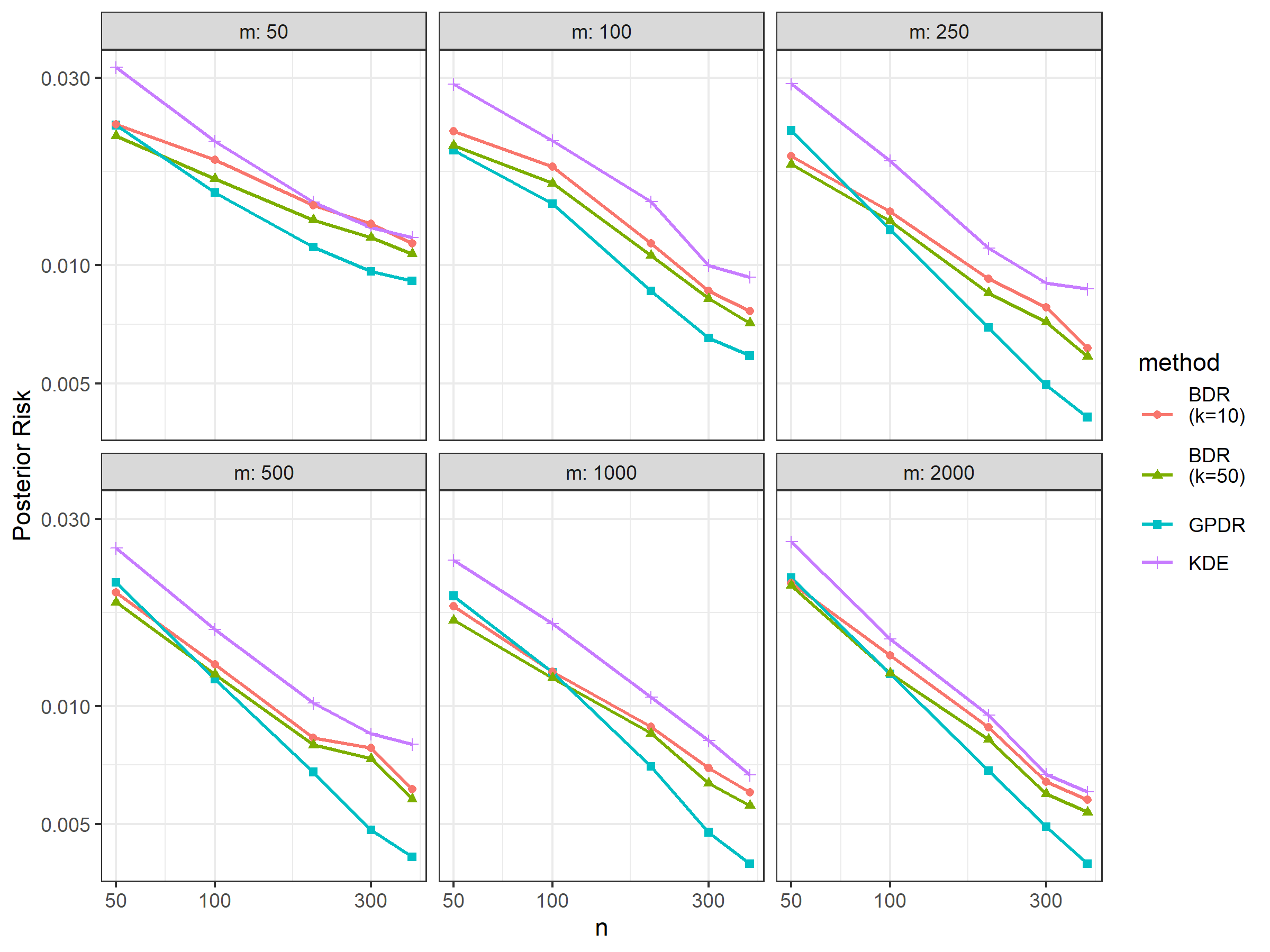
Figure 1: The empirical posterior risk for every combination of $n$ and $m$ under 100 runs, where $n$ stands for the number of subjects and $m$ is the number of samples for each subject. GPDR is for our Gaussian Process distribution regression model; KDE stands for its direct alternative (21) using kernel density estimated expectations; BDR stands for the Bayes distribution regression method suggested in Law et al. (2018), where $k$ is the number of landmark points.

6 NHANES activity data analysis

The National Health and Nutrition Examination Survey (NHANES) is a long standing survey study conducted by the Centers for Disease Control and Prevention and the National Center for Health Statistics to study the nutrition and health of the US population. Relatively recent samples (2003, 2005 cycles) collected physical activity data via hip worn accelerometers. The data consist of minute resolution records of activity intensity beginning from 12:01 a.m. the day after participants’ health examination. Subjects were instructed to wear the accelerometer for 7 consecutive days during the daytime, except when showering or bathing. The data used herein was processed and curated in the rnhanes package, as described in Leroux et al. (2019).

The database contains relatively high frequency activity data recorded from accelerometers. These are often summarized by a single measure of daily activity (see the discussion in Bai et al., 2016). However, it is of also interest to consider the functional shape of the activity as a time ordered function (Goldsmith et al., 2016). We further argue that it is also of interest to investigate time-invariant summaries of the data, to summarize the role of activity, whenever it occurred. Of course, summaries of the data, such as aggregate activity are time-invariant, but the question is what other information remains in the entire time course treated as if exchangeable. Therefore, we consider the activity counts as exchangeable covariates, as if repeated measures, ignoring the time-ordering of data points and assuming them to be samples from a subject-specific distribution. We then apply our method to perform distribution regression. We illustrate that in this setting we can have superior performance compared to typical functional data analysis which considers the time and not the distribution as informative.

The data is comprised of 2,719 subjects recorded in 2003-2004 & 2005-2006 NHANES survey cycles with activity count data for every minute during one week (i.e., there are $1,440=60$ minutes/hour $\times 24$ hours) points for every subject everyday. In this analysis, we use it to predict the age of subjects reported during the survey. Activity has been shown to be correlated with age, with Schrack et al. (2014) reporting an expected 1.3% decline in total activity per year. For simplicity, we use only the activity data on Friday, because empirically mean activity on this day had the highest correlation with age. Care should be taken in interpreting our results, since Smirnova et al. (2020) showed a high correlation between accelerometry estimated activity, in the NHANES dataset, and all cause mortality.

Denote the age of subject $i$ as $y_{i}$ and the log-transformed activity counts as $x_{ij}=\log(1+count_{ij})$ for every minute $j$. Consider two situations: 1) $x_{ij}$ as functional data with equally spaced time indices, $j$, via functional linear regression (FLR), 2) ignoring that $j$ corresponds to the $j^{th}$ time-point and treating $\{x_{ij}\}$ as exchangeable samples from some distribution, $z_{i}$, and utilizing distribution regression approaches. We will use both our Gaussian Process distribution regression (GPDR) with low rank approximation as described in section 4.1 as well as the Bayesian Linear Regression (BLR) method introduced in Law et al. (2018). The BLR model was chosen as it is a simplified version of the BDR model used in Section 5, which is computationally intensive. Of note, only the uncertainty in the regression function is modeled, while sampling uncertainty is not.

For functional analysis, we use penalized functional linear regression and smooth the curve using a 10 cubic spline basis with equally spaced knots. The penalization parameter is estimated from generalized cross validation. In the distribution regression situation we use the low rank approximation of Section 4.1 and set $k=10$ fixed. We further use a Matérn kernel with regularity 2.5 (thus is twice differentiable). As suggested in Kammann & Wand (2003), we set the scale parameter as the range $\max x_{ij}-\min x_{ij}$. Other parameters were fit from generalized cross validation. We use the same kernel for BLR method and set 10 and 50 evenly spaced landmark points in the range of $[\min x_{ij},\max x_{ij}]$. All other hyperparameters were set as the default values.

Each algorithm is evaluated using 5-fold cross validation. The mean R squared and its 95 % confidence interval are estimated from 500 independent runs. In each run the R squared in the validation data and record the average value across 5 folds. Results are shown in Table 1. The density regression method significantly outperforms the default functional regression method and does slightly better than the BLR method in Law et al. (2018). There is a roughly 26% improvement in out-of-sample R squared compared to functional linear regression and 6% improvements compared to the Bayesian linear regression.

	FLR	GPDR	BLR:10	BLR:50
R squared	14.7%	18.5 %	17.6 %	17.6 %
95% CI	(14.2 %, 15.0%)	(17.9 %, 18.8%)	(17.2 %, 17.8 %)	(17.2 %, 17.8 %)

Table 1: 5-fold cross validation results for different algorithms. FLR means functional linear model that respect the time order of the data. GPDR is our Gaussian Process distribution regression using low rank approximation method which ignoring any time information. BLR is the Bayesian linear regression model of Law et al. (2018) with 10 or 50 landmark points.

The results demonstrate that distribution regression is often worth considering, even if the data is functional in nature and not random samples from individual distributions. This clearly can happen when order invariant summaries of the data, rather than ordered functional summaries are more related to the outcome.

7 Discussion

We present a simple approach to regression using distribution-valued (repeated measures) covariate. We frame the model as a generalization of the typical Bayesian GP regression. This has several advantages. The method becomes simply a GP regression with the kernel averaged across repeated measures. We can obtain inference from the model directly using the observed covariate samples without having to estimate the subject-specific distributions or densities. All advantages of GP regression are retained, such as exploiting conjugacy in a Gibbs sampler and using low-rank GP approximations. The hierarchical formulation allows incorporating other subject-specific information like additional scalar-valued covariates and longitudinal or clustered data structures. Future work will explore these extensions in the context of specific applications.

Theoretically, we present a comprehensive, and to our knowledge, the first set of results for Bayesian distribution regression using GP. We show our method has the same optimal finite-sample error bounds of function estimation as the typical GP regression does, under the same assumptions on the function smoothness and kernel choice as long as the class of subject-specific distributions is separable, i.e., rich enough to identify the regression functions.

Supplementary Materials

S1 Proofs

S1.1 Definitions

In this manuscript, we will mainly study the Hölder space $C^{\alpha}[0,1]^{d}$ for $\alpha>0$. When writing $\alpha=k+\eta$, the space $C^{\alpha}[0,1]^{d}$ is the space of all functions supported in $[0,1]^{d}$, whose partial derivatives of orders $(l_{1},\cdots,l_{d})$ exist for all nonnegative integers $l_{1},\cdots,l_{d}$ such that $l_{1}+\cdots+l_{d}\leq k$ and for which the highest order partial derivatives are Hölder continuous with order $\eta$ ($f$ being Hölder continuous with order $\eta$ if $|f(x)-f(y)|\leq C\left\lVert x-y\right\rVert^{\eta}$ for all $x,y$ and some constant $C$) .

Another functional space we will study is the Sobolev space $H^{\alpha}[0,1]^{d}$ which contains all $[0,1]^{d}\rightarrow\mathbb{R}$ functions $f$ such that

$$\int_{\mathbb{R}^{d}}\left(1+\left\lVert\lambda\right\rVert^{2}\right)^{\alpha}\left|\hat{f}(\lambda)\right|^{2}d\lambda<\infty$$

where $\hat{f}$ is the Fourier transformation of $f$: $\hat{f}(\lambda)=(2\pi)^{-d}\int\exp(i\lambda^{T}t)f(t)dt$.

An order $\alpha$ Matérn kernel for $d$ dimensional process has the form:

$$K(s,t)=\int_{\mathbb{R}^{d}}\frac{e^{i\lambda^{T}(s-t)}}{(1+\left\lVert\lambda\right\rVert^{2})^{\alpha+d/2}}d\lambda.$$

S1.2 Strong separability of Dirichlet Process

of Lemma 1.

Using stick breaking representation, we know that the sample probability mass function $p(x)$ has the form

$$p(x)=\sum_{k=1}^{\infty}\beta_{k}\cdot\delta_{x_{k}}(x),$$ (S22)

where $\beta_{k}=\beta^{\prime}_{k}\prod_{i=1}^{k-1}(1-\beta_{i}^{\prime})$ for $\beta_{k}^{\prime}$ i.i.d follows $\text{Beta}(1,\alpha)$ and $x_{k}$ i.i.d follows $\mu$ with $\delta_{x}$ the point mass at $x$. Also it is clear that the mean measure for $\text{DP}(\mu,\alpha)$ is just $\mu$. Therefore for bounded $f$, we can directly calculate $\mathbb{E}_{z\sim\text{DP}(\mu,\alpha)}[(\mathbb{E}_{z}f)^{2}]$. We have:

$$\mathbb{E}_{z\sim\text{DP}(\mu,\alpha)}[(\mathbb{E}_{z}f)^{2}] =\mathbb{E}_{z\sim\text{DP}(\mu,\alpha)}\left[\left(\sum_{k=1}^{\infty}\beta_{k}f(x_{k})\right)^{2}\right]$$

$$=\mathbb{E}_{z\sim\text{DP}(\mu,\alpha)}\left[\sum_{ij}^{\infty}f(x_{i})f(x_{j})\beta_{i}\beta_{j}\right]$$

$$=\mathbb{E}_{\mu}f^{2}\cdot\sum_{i}\frac{2}{\alpha(1+\alpha)}\left(\frac{\alpha}{2+\alpha}\right)^{i}+(\mathbb{E}_{\mu}f)^{2}\sum_{i\neq j}\mathbb{E}[\beta_{i}\beta_{j}]$$

$$\geq\mathbb{E}_{\mu}f^{2}\cdot\sum_{i}\frac{2}{\alpha(1+\alpha)}\left(\frac{\alpha}{2+\alpha}\right)^{i}=\frac{1}{1+\alpha}\mathbb{E}_{\mu}f^{2}$$

Therefore $\text{DP}(\mu,\alpha)$ strongly separates the bounded functions with constant $C=1+\alpha$. ∎

S1.3 Risk Decomposition

The way we prove the theorems is to do risk decomposition. Consider the Gaussian process model with unknown true distributions $z_{i}$:

$$f\sim GP(0,K)$$ (S23)

$$y_{i}\sim\mathcal{N}\left(\mathbb{E}_{z_{i}}f,\sigma^{2}\right)$$ (S24)

the posterior of which is denoted as $\Pi_{n}(f|\mathbb{Z}_{n})$. Then the risk term 9 can be decomposed into:

$$R_{n}=R_{n}^{0}+R_{n}^{1}=\mathbb{E}_{f_{0}}\int||f-f_{0}||^{2}d\Pi_{n}(f|\mathbb{Z}_{n})+\left(\mathbb{E}_{f_{0}}\int||f-f_{0}||^{2}(d\Pi_{n}(f|\mathbb{D}_{n})-d\Pi_{n}(f|\mathbb{Z}_{n}))\right)$$ (S25)

where $\left\lVert\cdot\right\rVert$ can be empirical norm $\left\lVert\cdot\right\rVert_{n}$ and $L_{2}$ norm $\left\lVert\cdot\right\rVert_{2}$. We can bound $\mathbb{R}^{0}_{n}$ using similar method as in Van Der Vaart & Van Zanten (2011) and bound $\mathbb{R}^{1}_{n}$ through a direct computation.

S1.4 Bound $R_{n}^{1}$ for $L_{2}$ norm $\left\lVert\cdot\right\rVert_{2}$

A naive bound for $R_{n}^{1}$ is to directly calculate it out:

$$R_{n}^{1} =\mathbb{E}_{f_{0}}\int||f-f_{0}||^{2}(d\Pi_{n}(f|\mathbb{D}_{n})-d\Pi_{n}(f|\mathbb{Z}_{n}))$$

$$=\mathbb{E}_{f_{0}}\int_{[0,1]^{d}}\left(\mathbb{E}_{f|\mathbb{D}_{n}}(f-f_{0})^{2}(s)-\mathbb{E}_{f|\mathbb{Z}_{n}}(f-f_{0})^{2}(s)\right)ds$$

$$=\mathbb{E}_{f_{0}}\int_{[0,1]^{d}}\left(\mathbb{E}_{f|\mathbb{D}_{n}}(f^{2}(s)-2f(s)f_{0}(s))-\mathbb{E}_{f|\mathbb{Z}_{n}}(f^{2}(s)-2f(s)f_{0}(s))\right)ds$$

$$=\mathbb{E}_{f_{0}}\int_{[0,1]^{d}}\text{Var}(f(s)|\mathbb{D}_{n})-\text{Var}(f(s)|\mathbb{Z}_{n})+\mathbb{E}^{2}(f(s)|\mathbb{D}_{n})-\mathbb{E}^{2}(f(s)|\mathbb{Z}_{n})$$

$$\hskip 50.00008pt-2f_{0}(s)\left(\mathbb{E}(f(s)|\mathbb{D}_{n})-\mathbb{E}(f(s)|\mathbb{Z}_{n})\right)ds$$

$$=\mathbb{E}_{f_{0}}\int_{[0,1]^{d}}V(s)+E_{2}(s)-2f_{0}(s)E_{1}(s)ds$$

where $V(s)=\text{Var}(f(s)|\mathbb{D}_{n})-\text{Var}(f(s)|\mathbb{Z}_{n})$, $E_{1}(s)=\mathbb{E}_{\bm{\varepsilon}}\left[\mathbb{E}(f(s)|\mathbb{D}_{n})-\mathbb{E}(f(s)|\mathbb{Z}_{n})\right]$ and $E_{2}(s)=\mathbb{E}_{\bm{\varepsilon}}\left[\mathbb{E}^{2}(f(s)|\mathbb{D}_{n})-\mathbb{E}^{2}(f(s)|\mathbb{Z}_{n})\right]$. All exchange of integral and expectation above should be legal because all functions are clearly bounded by a constant if fixing $n$.

Borrow similar notation as in Szabó et al. (2016); Caponnetto & De Vito (2007). Let $\mathcal{H}$ be the RKHS of the GP kernel $K$ with inner product $\langle\cdot,\cdot\rangle$. Let

$$\mu_{z}(s)=\int K(s,t)dz(t)$$

be the kernel mean embedding of distribution $z$. Denote:

$$T_{\bm{z}}=\frac{1}{n}\sum_{i=1}^{n}\mu_{z_{i}}\langle\mu_{z_{i}},\cdot\rangle,\hskip 20.00003ptg_{\bm{z}}=\frac{1}{n}\sum_{i=1}^{n}y_{i}\mu_{z_{i}},\hskip 20.00003pt\phi_{\bm{z}}=\frac{1}{n}\sum_{i=1}^{n}\mu_{z_{i}}\otimes\mu_{z_{i}}$$

where $(f_{1}\otimes f_{2})(s,t)=f_{1}(s)f_{2}(t)$ and $z_{i},y_{i}$ are the true distribution and response for subject $i$. Naturally, $\mathcal{H}\otimes\mathcal{H}$ would be the closure of set $\{f_{1}\otimes f_{2}:f_{1}\in\mathcal{H},f_{2}\in\mathcal{H}\}$, equipped with inner product as continuous extension of $\langle f_{1}\otimes f_{2},g_{1}\otimes g_{2}\rangle=\langle f_{1},g_{1}\rangle\langle f_{2},g_{2}\rangle$. Then we know that $g_{\bm{z}}\in\mathcal{H}$ and $T_{\bm{z}}:\mathcal{H}\rightarrow\mathcal{H}$ is Hermitian. Similarly we can define $T_{\hat{\bm{z}}},g_{\hat{\bm{z}}},\phi_{\hat{\bm{z}}}$ by changing true distribution $z_{i}$ to empirical distribution $\hat{z}_{i}$ based on the samples $\{x_{ij}\}$ , and they have the same properties. Following these notations, Gaussian process has following posterior (Caponnetto & De Vito, 2007):

$$f\ |\ \mathbb{Z}_{n} \sim GP\left((T_{\bm{z}}+\sigma_{n}^{2})^{-1}g_{\bm{z}},\ K-\left[(T_{\bm{z}}+\sigma_{n}^{2})^{-1}\otimes\text{Id}\right]\phi_{\bm{z}}\right)$$ (S26)

$$f\ |\ \mathbb{D}_{n} \sim GP\left((T_{\hat{\bm{z}}}+\sigma_{n}^{2})^{-1}g_{\hat{\bm{z}}},\ K-\left[(T_{\hat{\bm{z}}}+\sigma_{n}^{2})^{-1}\otimes\text{Id}\right]\phi_{\hat{\bm{z}}}\right)$$ (S27)

where $\sigma_{n}^{2}=\sigma^{2}/n$ and Id is the identity operator. Here the operator $T_{1}\otimes T_{2}:\mathcal{H}\otimes\mathcal{H}\rightarrow\mathcal{H}\otimes\mathcal{H}$ is naturally defined through continuous extension of $(T_{1}\otimes T_{2})(f_{1}\otimes f_{2})=T_{1}(f_{1})\otimes T_{2}(f_{2})$. Denote $\hat{z}_{i}$ being the empirical distribution from samples $x_{ij}$, $f_{\bm{z}}=(T_{\bm{z}}+\sigma_{n}^{2})^{-1}g_{\bm{z}}$ and $f_{\hat{\bm{z}}}=(T_{\hat{\bm{z}}}+\sigma_{n}^{2})^{-1}g_{\hat{\bm{z}}}$. Also $M_{\bm{z}}=\left[(T_{\bm{z}}+\sigma_{n}^{2})^{-1}\otimes\text{Id}\right]\phi_{\bm{z}}$ and $M_{\hat{\bm{z}}}=\left[(T_{\hat{\bm{z}}}+\sigma_{n}^{2})^{-1}\otimes\text{Id}\right]\phi_{\hat{\bm{z}}}$. Therefore $M_{\bm{z}},M_{\hat{\bm{z}}}\in\mathcal{H}\otimes\mathcal{H}$. Now we can bound $R_{n}^{1}$ step by step. In the following sections, we denote $K_{s}$ as the function $K_{s}(t)=K(s,t)$.

S1.5 Step 1: Bound $V(s)$

We have $V(s)=M_{\bm{z}}(s,s)-M_{\hat{\bm{z}}}(s,s)$. It is easy to observe that

$$M_{\bm{z}}(s,s) =\langle M_{\bm{z}},K_{s}\otimes K_{s}\rangle=\left\langle\frac{1}{n}\sum_{i=1}^{n}(T_{\bm{z}}+\sigma^{2}_{n})^{-1}\mu_{z_{i}}\langle\mu_{z_{i}},K_{s}\rangle,K_{s}\right\rangle$$

$$=\left\langle(T_{\bm{z}}+\sigma^{2}_{n})^{-1}T_{\bm{z}}K_{s},K_{s}\right\rangle$$

The second equation comes from the definition of $\mathcal{H}\otimes\mathcal{H}$. Therefore

$$|V(s)| =\left|\left\langle((T_{\bm{z}}+\sigma^{2}_{n})^{-1}T_{\bm{z}}-(T_{\hat{\bm{z}}}+\sigma^{2}_{n})^{-1}T_{\hat{\bm{z}}})K_{s},K_{s}\right\rangle\right|$$

$$\leq\kappa\left\lVert(T_{\bm{z}}+\sigma^{2}_{n})^{-1}T_{\bm{z}}-(T_{\hat{\bm{z}}}+\sigma^{2}_{n})^{-1}T_{\hat{\bm{z}}}\right\rVert_{\mathcal{L(H)}}$$

$$=\kappa\sigma^{2}_{n}\left\lVert(T_{\hat{\bm{z}}}+\sigma^{2}_{n})^{-1}-(T_{\bm{z}}+\sigma^{2}_{n})^{-1}\right\rVert_{\mathcal{L(H)}}$$

$$=\kappa\sigma^{2}_{n}\left\lVert(T_{\hat{\bm{z}}}+\sigma^{2}_{n})^{-1}(T_{\bm{z}}-T_{\hat{\bm{z}}})(T_{\bm{z}}+\sigma^{2}_{n})^{-1}\right\rVert_{\mathcal{L(H)}}\leq\frac{\kappa}{\sigma_{n}^{2}}\left\lVert(T_{\bm{z}}-T_{\hat{\bm{z}}})\right\rVert_{\mathcal{L(H)}}$$

for operator norm $\left\lVert\cdot\right\rVert_{\mathcal{L(H)}}$. Notice that $\kappa$ is the upper bound for the kernel $K$. To bound $\left\lVert(T_{\bm{z}}-T_{\hat{\bm{z}}})\right\rVert_{\mathcal{L(H)}}$, we have:

$$\left\lVert T_{\bm{z}}-T_{\hat{\bm{z}}}\right\rVert_{\mathcal{L(H)}}^{2} \leq\frac{1}{n}\sum_{i=1}^{n}\left\lVert\mu_{z_{i}}\langle\mu_{z_{i}},\cdot\rangle-\mu_{\hat{z}_{i}}\langle\mu_{\hat{z}_{i}},\cdot\rangle\right\rVert_{\mathcal{L(H)}}^{2}$$

And for every $\left\lVert\mu_{z_{i}}\langle\mu_{z_{i}},\cdot\rangle-\mu_{\hat{z}_{i}}\langle\mu_{\hat{z}_{i}},\cdot\rangle\right\rVert$, apply it to arbitrary function $f$.

$$\left\lVert\mu_{z_{i}}\langle\mu_{z_{i}},f\rangle-\mu_{\hat{z}_{i}}\langle\mu_{\hat{z}_{i}},f\rangle\right\rVert_{\mathcal{H}}^{2} =\left\lVert(\mu_{z_{i}}-\mu_{\hat{z}_{i}})\langle\mu_{z_{i}},f\rangle+\mu_{\hat{z}_{i}}\langle\mu_{z_{i}}-\mu_{\hat{z}_{i}},f\rangle\right\rVert_{\mathcal{H}}^{2}$$

$$\leq\left\lVert f\right\rVert_{\mathcal{H}}^{2}\left(\left(\left\lVert\mu_{z_{i}}\right\rVert_{\mathcal{H}}^{2}+\left\lVert\mu_{\hat{z}_{i}}\right\rVert_{\mathcal{H}}^{2}\right)\left\lVert\mu_{z_{i}}-\mu_{\hat{z}_{i}}\right\rVert_{\mathcal{H}}^{2}\right)$$

$$\leq 2\kappa\left\lVert f\right\rVert_{\mathcal{H}}^{2}\left\lVert\mu_{z_{i}}-\mu_{\hat{z}_{i}}\right\rVert_{\mathcal{H}}^{2}$$

Therefore $\left\lVert T_{\bm{z}}-T_{\hat{\bm{z}}}\right\rVert_{\mathcal{L(H)}}^{2}\leq\frac{2\kappa}{n}\sum_{i}\left\lVert\mu_{z_{i}}-\mu_{\hat{z}_{i}}\right\rVert_{\mathcal{H}}^{2}$. And

$$\left|\mathbb{E}\int_{[0,1]^{d}}V(s)ds\right| \leq\frac{\kappa}{\sigma_{n}^{2}}\mathbb{E}\left\lVert(T_{\bm{z}}-T_{\hat{\bm{z}}})\right\rVert_{\mathcal{L(H)}}\leq\frac{\sqrt{2}\kappa^{3/2}}{\sigma_{n}^{2}}\sqrt{\mathbb{E}\left\lVert\mu_{z_{i}}-\mu_{\hat{z}_{i}}\right\rVert_{\mathcal{H}}^{2}}$$

$$=\frac{\sqrt{2}\kappa^{3/2}}{\sigma_{n}^{2}}\sqrt{\mathbb{E}_{z_{i}}\mathbb{E}_{x_{ij}}\left\lVert\frac{1}{m}\sum_{j}K_{x_{ij}}-\mu_{z_{i}}\right\rVert_{\mathcal{H}}^{2}}$$

$$=\frac{\sqrt{2}\kappa^{3/2}}{\sigma_{n}^{2}}\sqrt{\mathbb{E}_{z_{i}}\left[\frac{1}{m}\mathbb{E}_{x_{ij}}\left\lVert K_{x_{ij}}-\mu_{z_{i}}\right\rVert_{\mathcal{H}}^{2}\right]}\leq\frac{2\sqrt{2}\kappa^{2}}{\sigma_{n}^{2}\sqrt{m}}$$ (S28)

S1.6 Step 2: Bound $E_{1}(s)$

One main difficulty for the bound here is that we don’t assume $f_{0}$ lying in the RKHS of kernel $K$. In fact, when optimal rate is achieved with $\beta=\alpha$, the RKHS $\mathcal{H}_{K}$ contains all $(\beta+1/2)$-regular functions, which means $f_{0}\not\in\mathcal{H}_{K}$.

In the situation $f_{0}\not\in\mathcal{H}_{K}$, from Lemma 4 of Van Der Vaart & Van Zanten (2011) we know that for order $\alpha$ Matérn kernel $K$ and $\beta$-regular $f_{0}$ with $\beta\leq\alpha$ we can always find $h\in\mathcal{H}_{K}$ such that:

$$\inf_{\left\lVert h-f_{0}\right\rVert_{\infty}<\varepsilon}\left\lVert h\right\rVert_{\mathcal{H}}^{2}\leq C_{\alpha}\left(\frac{1}{\varepsilon}\right)^{(2\alpha-2\beta+d)/\beta}$$ (S29)

for arbitrary small $\varepsilon$ and constant $C_{\alpha}$ depending only on $\alpha$ and $f_{0}$. Now we use equation S29 to find a $f_{0}^{\gamma}\in\mathcal{H}$ such that $\left\lVert f_{0}^{\gamma}-f_{0}\right\rVert_{\infty}\leq n^{-\gamma}$ and $\left\lVert f_{0}^{\gamma}\right\rVert_{\mathcal{H}}\leq 2C_{\alpha}n^{(2\alpha-2\beta+d)\gamma/2\beta}$. We will determine $\gamma$ at the end of the proof. Then we have $\mathbb{E}_{\varepsilon_{i}}y_{i}=\mathbb{E}_{z_{i}}f_{0}=\mathbb{E}_{z_{i}}f_{0}^{\gamma}+\mathbb{E}_{z_{i}}(f_{0}-f_{0}^{\gamma})=\langle\mu_{z_{i}},f_{0}^{\gamma}\rangle+\mathbb{E}_{z_{i}}(f_{0}-f_{0}^{\gamma})$. Denote $r_{i}=\mathbb{E}_{z_{i}}(f_{0}-f_{0}^{\gamma})$, we have $|r_{i}|\leq n^{-\gamma}$ and:

$$\mathbb{E}_{\bm{\varepsilon}}(T_{\bm{z}}+\sigma_{n}^{2})^{-1}g_{\bm{z}} =(T_{\bm{z}}+\sigma_{n}^{2})^{-1}\left(\frac{1}{n}\sum_{i}(\langle\mu_{z_{i}},f_{0}^{\gamma}\rangle\mu_{z_{i}}+r_{i}\mu_{z_{i}})\right)$$

$$=(T_{\bm{z}}+\sigma_{n}^{2})^{-1}T_{\bm{z}}f_{0}^{\gamma}+\frac{1}{n}\sum_{i}r_{i}(T_{\bm{z}}+\sigma_{n}^{2})^{-1}\mu_{z_{i}}$$

And similarly:

$$\mathbb{E}_{\bm{\varepsilon}}(T_{\hat{\bm{z}}}+\sigma_{n}^{2})^{-1}g_{\hat{\bm{z}}} =(T_{\hat{\bm{z}}}+\sigma_{n}^{2})^{-1}\left(\frac{1}{n}\sum_{i}(\langle\mu_{z_{i}},f_{0}^{\gamma}\rangle\mu_{\hat{z}_{i}}+r_{i}\mu_{\hat{z}_{i}})\right)$$

$$=(T_{\hat{\bm{z}}}+\sigma_{n}^{2})^{-1}T_{\hat{\bm{z}}}f_{0}^{\gamma}+\frac{1}{n}\sum_{i}(r_{i}+d_{i})(T_{\hat{\bm{z}}}+\sigma_{n}^{2})^{-1}\mu_{\hat{z}_{i}}$$

where $d_{i}=\langle\mu_{z_{i}}-\mu_{\hat{z}_{i}},f_{0}^{\gamma}\rangle$.

Therefore

$$|E_{1}(s)| =\left|\langle E_{1},K_{s}\rangle\right|\leq\sqrt{\kappa}\left\lVert E_{1}\right\rVert_{\mathcal{H}}$$

$$\leq\sqrt{\kappa}\left\lVert(T_{\bm{z}}+\sigma_{n}^{2})^{-1}T_{\bm{z}}-(T_{\hat{\bm{z}}}+\sigma_{n}^{2})^{-1}T_{\hat{\bm{z}}}\right\rVert_{\mathcal{L(H)}}\left\lVert f_{0}^{\gamma}\right\rVert_{\mathcal{H}}$$

$$\hskip 20.00003pt+\sqrt{\kappa}\left\lVert\frac{1}{n}\sum_{i}d_{i}(T_{\hat{\bm{z}}}+\sigma_{n}^{2})^{-1}\mu_{\hat{z}_{i}}\right\rVert_{\mathcal{H}}+\sqrt{\kappa}\left\lVert\frac{1}{n}\sum_{i}r_{i}(T_{\bm{z}}+\sigma_{n}^{2})^{-1}(\mu_{z_{i}}-\mu_{\hat{z}_{i}})\right\rVert_{\mathcal{H}}$$

$$\hskip 20.00003pt+\sqrt{\kappa}\left\lVert\frac{1}{n}\sum_{i}r_{i}((T_{\bm{z}}+\sigma_{n}^{2})^{-1}-(T_{\hat{\bm{z}}}+\sigma_{n}^{2})^{-1})\mu_{\hat{z}_{i}}\right\rVert_{\mathcal{H}}$$

$$\leq\left(\frac{2C_{\alpha}\sqrt{\kappa}}{\sigma_{n}^{2}}\left\lVert T_{\bm{z}}-T_{\hat{\bm{z}}}\right\rVert_{\mathcal{L(H)}}+\frac{2C_{\alpha}\kappa}{\sigma_{n}^{2}n}\sum_{i}\left\lVert\mu_{z_{i}}-\mu_{\hat{z_{i}}}\right\rVert_{\mathcal{H}}\right)n^{\frac{(2\alpha-2\beta+d)\gamma}{2\beta}}$$

$$\hskip 20.00003pt+\left(\frac{\sqrt{\kappa}}{\sigma_{n}^{2}n}\sum_{i}\left\lVert\mu_{z_{i}}-\mu_{\hat{z_{i}}}\right\rVert_{\mathcal{H}}+\frac{\kappa}{\sigma_{n}^{4}}\left\lVert T_{\bm{z}}-T_{\hat{\bm{z}}}\right\rVert_{\mathcal{L(H)}}\right)n^{-\gamma}$$

Using the bounds derived in previous step, we have:

$$\left|\mathbb{E}\int_{[0,1]^{d}}2f_{0}(s)E_{1}(s)ds\right|\leq\frac{16C_{0}C_{\alpha}\kappa^{3/2}}{\sigma_{n}^{2}\sqrt{m}}n^{\frac{(2\alpha-2\beta+d)\gamma}{2\beta}}+\frac{4C_{0}\kappa}{\sigma_{n}^{2}\sqrt{m}}n^{-\gamma}+\frac{4\sqrt{2}\kappa^{2}}{\sigma_{n}^{4}\sqrt{m}}n^{-\gamma}$$

where $C_{0}$ is the upper bound of $|f_{0}|$ which must exists, because we assume $f_{0}$ regular (hence continuous) in a compact set. The rate can be improved when $f_{0}\in\mathcal{H}_{K}$ ($\beta\geq\alpha+1/2$), in which case $f_{0}^{\gamma}$ can directly be $f_{0}$, making $r_{i}=0$ and $\left\lVert f_{0}^{\gamma}\right\rVert$ constant. We have:

$$\left|\mathbb{E}\int_{[0,1]^{d}}2f_{0}(s)E_{1}(s)ds\right|\leq\frac{16C_{0}C_{\alpha}\kappa^{3/2}}{\sigma_{n}^{2}\sqrt{m}}$$

S1.7 Step 3: Bound $E_{2}(s)$

Using the same notation as in Step 2. In the situation $f_{0}\not\in\mathcal{H}_{K}$, we denote:

$$A =(T_{\bm{z}}+\sigma_{n}^{2})^{-1}T_{\bm{z}}f_{0}^{\gamma},\hskip 10.00002ptB=\frac{1}{n}\sum_{i}\varepsilon_{i}(T_{\bm{z}}+\sigma_{n}^{2})^{-1}\mu_{z_{i}},\hskip 10.00002ptC=\frac{1}{n}\sum_{i}r_{i}(T_{\bm{z}}+\sigma_{n}^{2})^{-1}\mu_{z_{i}}$$

$$\hat{A} =(T_{\hat{\bm{z}}}+\sigma_{n}^{2})^{-1}T_{\hat{\bm{z}}}f_{0}^{\gamma},\hskip 10.00002pt\hat{B}=\frac{1}{n}\sum_{i}\varepsilon_{i}(T_{\hat{\bm{z}}}+\sigma_{n}^{2})^{-1}\mu_{\hat{z}_{i}},\hskip 10.00002pt\hat{C}=\frac{1}{n}\sum_{i}(r_{i}+d_{i})(T_{\hat{\bm{z}}}+\sigma_{n}^{2})^{-1}\mu_{\hat{z}_{i}}$$

Then $E_{2}=\mathbb{E}_{\bm{\varepsilon}}\left[(A+B+C)^{2}-(\hat{A}+\hat{B}+\hat{C})^{2}\right]$. Easy to see $\mathbb{E}_{\bm{\varepsilon}}\left[B(A+C)+\hat{B}(\hat{A}+\hat{C})\right]=0$. Because $\varepsilon_{i}$ is mean 0 and independent of any $z_{i}$ and $x_{ij}$. Therefore

$$E_{2}=(A+C+\hat{A}+\hat{C})(A-\hat{A}+C-\hat{C})+\mathbb{E}_{\bm{\varepsilon}}\left[B^{2}-\hat{B}^{2}\right]$$

For the first part

$$|(A+C+\hat{A}+\hat{C})(A-\hat{A}+C-\hat{C})|(s)=|\langle A+C+\hat{A}+\hat{C},K_{s}\rangle\langle A-\hat{A}+C-\hat{C},K_{s}\rangle|$$

$$\hskip 60.00009pt\leq\kappa\left(\left\lVert A\right\rVert_{\mathcal{H}}+\left\lVert\hat{A}\right\rVert_{\mathcal{H}}+\left\lVert C\right\rVert_{\mathcal{H}}+\left\lVert\hat{C}\right\rVert_{\mathcal{H}}\right)\left\lVert E_{1}\right\rVert_{\mathcal{H}}$$

$$\hskip 60.00009pt\leq\kappa\left\lVert E_{1}\right\rVert_{\mathcal{H}}\left(2\left\lVert f_{0}^{\gamma}\right\rVert_{\mathcal{H}}+\frac{2\sqrt{\kappa}}{\sigma_{n}^{2}}n^{-\gamma}+\frac{\sqrt{\kappa}\left\lVert f_{0}^{\gamma}\right\rVert_{\mathcal{H}}}{\sigma_{n}^{2}n}\sum_{i}\left\lVert\mu_{z_{i}}-\mu_{\hat{z}_{i}}\right\rVert_{\mathcal{H}}\right)$$

We can use the same bound for $E_{1}$ and notice that:

$$\mathbb{E}\left[\frac{\left\lVert T_{\bm{z}}-T_{\hat{\bm{z}}}\right\rVert_{\mathcal{L(H)}}}{n}\sum_{i}\left\lVert\mu_{z_{i}}-\mu_{\hat{z}_{i}}\right\rVert_{\mathcal{H}}\right]\leq\sqrt{\mathbb{E}\left\lVert T_{\bm{z}}-T_{\hat{\bm{z}}}\right\rVert_{\mathcal{L(H)}}^{2}\mathbb{E}\left\lVert\mu_{z_{i}}-\mu_{\hat{z}_{i}}\right\rVert_{\mathcal{H}}^{2}}=O\left(\frac{1}{m}\right)$$

$$\mathbb{E}\left[\left(\frac{1}{n}\sum_{i}\left\lVert\mu_{z_{i}}-\mu_{\hat{z}_{i}}\right\rVert_{\mathcal{H}}\right)\left(\frac{1}{n}\sum_{i}\left\lVert\mu_{z_{i}}-\mu_{\hat{z}_{i}}\right\rVert_{\mathcal{H}}\right)\right]\leq\sqrt{\mathbb{E}\left\lVert\mu_{z_{i}}-\mu_{\hat{z}_{i}}\right\rVert_{\mathcal{H}}^{2}\mathbb{E}\left\lVert\mu_{z_{i}}-\mu_{\hat{z}_{i}}\right\rVert_{\mathcal{H}}^{2}}=O\left(\frac{1}{m}\right)$$

For the second part, we have (notice that $(T_{\bm{z}}+\sigma_{n}^{2})^{-1}$ is Hermitian):

$$\mathbb{E}_{\bm{\varepsilon}}[B^{2}](s) =\frac{1}{n^{2}}\sum_{i}\sigma^{2}\langle(T_{\bm{z}}+\sigma_{n}^{2})^{-1}\mu_{z_{i}},K_{s}\rangle\langle\mu_{z_{i}},(T_{\bm{z}}+\sigma_{n}^{2})^{-1}K_{s}\rangle$$

$$=\frac{\sigma^{2}}{n}\langle(T_{\bm{z}}+\sigma_{n}^{2})^{-2}T_{\bm{z}}K_{s},K_{s}\rangle$$

and

$$|\mathbb{E}_{\bm{\varepsilon}}[B^{2}-\hat{B}^{2}](s)| \leq\frac{\sigma^{2}\kappa}{n}\left\lVert(T_{\bm{z}}+\sigma_{n}^{2})^{-2}T_{\bm{z}}-(T_{\hat{\bm{z}}}+\sigma_{n}^{2})^{-2}T_{\hat{\bm{z}}}\right\rVert_{\mathcal{L(H)}}$$

$$\leq\kappa\sigma_{n}^{2}\left\lVert((T_{\bm{z}}+\sigma_{n}^{2})^{-1}-(T_{\hat{\bm{z}}}+\sigma_{n}^{2})^{-1})(T_{\bm{z}}+\sigma_{n}^{2})^{-1}T_{\bm{z}}\right\rVert_{\mathcal{L(H)}}$$

$$\hskip 10.00002pt+\kappa\sigma_{n}^{2}\left\lVert(T_{\bm{z}}+\sigma_{n}^{2})^{-1}((T_{\bm{z}}+\sigma_{n}^{2})^{-1}T_{\bm{z}}-(T_{\hat{\bm{z}}}+\sigma_{n}^{2})^{-1}T_{\hat{\bm{z}}})\right\rVert_{\mathcal{L(H)}}$$

$$\leq\frac{2\kappa}{\sigma_{n}^{2}}\left\lVert T_{\bm{z}}-T_{\hat{\bm{z}}}\right\rVert_{\mathcal{L(H)}}$$

Therefore, using bound in equation S28 and ignoring the constant term, we have (recall that $\left\lVert f_{0}^{\gamma}\right\rVert_{\mathcal{H}}=O(n^{(2\alpha-2\beta+d)\gamma/2\beta})$):

$$\left|\mathbb{E}\int_{[0,1]^{d}}E_{2}(s)ds\right| \leq C(\alpha,\kappa,f_{0})\left(\frac{1}{\sigma_{n}^{2}\sqrt{m}}n^{\frac{(2\alpha-2\beta+d)\gamma}{\beta}}+\frac{1}{\sigma_{n}^{4}\sqrt{m}}n^{-\gamma+\frac{(2\alpha-2\beta+d)\gamma}{2\beta}}\right.$$ (S30)

$$\hskip 10.00002pt+\left.\frac{1}{\sigma^{6}_{n}\sqrt{m}}n^{-2\gamma}+\frac{1}{\sigma_{n}^{4}m}n^{\frac{(2\alpha-2\beta+d)\gamma}{\beta}}+\frac{1}{\sigma_{n}^{6}m}n^{-\gamma+\frac{(2\alpha-2\beta+d)\gamma}{2\beta}}\right)$$ (S31)

for some constant $C(\alpha,\kappa,f_{0})$ depending only on $\alpha,\kappa,f_{0}$.

Similarly the rate can be improved if $f_{0}\in\mathcal{H}_{K}$, where $f_{0}^{\gamma}$ can directly be $f_{0}$, making $r_{i}=0$ and $\left\lVert f_{0}^{\gamma}\right\rVert$ constant. We have:

$$\left|\mathbb{E}\int_{[0,1]^{d}}E_{2}(s)ds\right| \leq\frac{C(\kappa,f_{0})}{\sigma^{2}_{n}\sqrt{m}}$$ (S32)

given $\sigma^{2}_{n}\sqrt{m}\to\infty$. Notice again that $\sigma_{n}^{2}=\sigma^{2}/n$.

S1.8 Combine Together

Combine all 3 steps above we have:

$$R^{1}_{n}=O\left(\frac{n}{\sqrt{m}}\right)$$ (S33)

if $f_{0}\in\mathcal{H}_{K}$ ($\beta\geq\alpha+1/2$). And if $f_{0}\not\in\mathcal{H}_{K}$ we would get a more complex and worse rate as:

$$R^{1}_{n}=O\left(\frac{n^{1+\frac{(2\alpha-2\beta+d)\gamma}{2\beta}}}{\sqrt{m}}+\frac{n^{2-\gamma+\frac{(2\alpha-2\beta+d)\gamma}{2\beta}}}{\sqrt{m}}+\frac{n^{3-2\gamma}}{\sqrt{m}}\right)$$ (S34)

given $n/\sqrt{m}\to 0$. Therefore when $\alpha=\beta$, setting $\gamma=1$ we get that $R^{1}_{n}=O(n^{-2\beta/(2\beta+d)})$ if $m=\Omega\left(n^{2+\frac{d}{\beta}+\frac{4\beta}{2\beta+d}}\right)$.

S1.9 Bound $R_{n}^{1}$ for empirical norm $\left\lVert\cdot\right\rVert_{n}$

Denote $\hat{\mathcal{Z}}$ as the empirical distributional process support only on $n$ points of $z_{i}$. We have:

$$R_{n}^{1} =\mathbb{E}_{f_{0}}\int\left\lVert f-f_{0}\right\rVert_{n}^{2}(d\Pi_{n}(f|\mathbb{D}_{n})-d\Pi_{n}(f|\mathbb{Z}_{n}))$$

$$=\mathbb{E}_{f_{0}}\int\mathbb{E}_{z\sim\hat{\mathcal{Z}}}[\mathbb{E}_{z}(f-f_{0})\mathbb{E}_{z}(f-f_{0})](d\Pi_{n}(f|\mathbb{D}_{n})-d\Pi_{n}(f|\mathbb{Z}_{n}))$$

$$=\mathbb{E}_{f_{0}}\mathbb{E}_{z\sim\hat{\mathcal{Z}}}\int\left[\int(f-f_{0})(s)(f-f_{0})(t)dz(s)dz(t)\right](d\Pi_{n}(f|\mathbb{D}_{n})-d\Pi_{n}(f|\mathbb{Z}_{n}))$$

$$=\mathbb{E}_{f_{0}}\mathbb{E}_{z\sim\hat{\mathcal{Z}}}\int(\mathbb{E}_{f|\mathbb{D}_{n}}-\mathbb{E}_{f|\mathbb{Z}_{n}})[f(s)f(t)]-2f_{0}(s)(\mathbb{E}_{f|\mathbb{D}_{n}}-\mathbb{E}_{f|\mathbb{Z}_{n}})[f(t)]\ dz(s)dz(t)$$

It is not hard to see one can use exactly the same method as in section S1.4 to get the same bound as for term $|(\mathbb{E}_{f|\mathbb{D}_{n}}-\mathbb{E}_{f|\mathbb{Z}_{n}})[f(s)f(t)]-2f_{0}(s)(\mathbb{E}_{f|\mathbb{D}_{n}}-\mathbb{E}_{f|\mathbb{Z}_{n}})[f(t)]|$ with every $s,t$ pair and therefore we can get the same overall bounds as for $\left\lVert\cdot\right\rVert_{2}$.

S1.10 Bound $R^{0}_{n}$

We would use the method described in Van Der Vaart & Van Zanten (2011) to bound $R^{0}_{n}$, by extending it to non-parametric GP regression on the space of distributions. To do that we need to rewrite the model S23-S24 into a typical Gaussian process regression in metric space. Consider:

$$y_{i}=F_{0}(z_{i})+\varepsilon_{i}$$ (S35)

where $z_{i}$ is the individual distribution for subject $i$ and $F_{0}$ is an element in linear space $\mathcal{B}$. such that there exists an bijection $\pi$ from $\mathcal{B}$ to $\mathcal{C}_{0}$: the bounded continuous function on $[0,1]^{d}$ and $\forall F\in\mathcal{B},z\in\mathcal{S}:\ F(z)=\mathbb{E}_{z}\pi(F)$. Naturally we give $\mathcal{B}$ a norm that $\left\lVert F\right\rVert_{\mathcal{B}}=\left\lVert\pi(F)\right\rVert_{\infty}$ and it is clear that $|F(z)|\leq\left\lVert F\right\rVert_{\mathcal{B}}$ for all $z$. When it is not misleading, we will also denote $\pi(F)$ simply as $f$. Similarly $f_{0}$ for $\pi(F_{0})$ and any other super-sub-script.

It is clear that if $\mathcal{Z}$ weakly separates $\mathcal{C}_{0}$, $\pi$ would be an isomorphism between $\mathcal{B}$ and $\mathcal{C}_{0}$. Because $\pi$ would be a bijection with $\left\lVert F\right\rVert_{\mathcal{B}}=\left\lVert\pi(F)\right\rVert_{\infty}$. Hence $\mathcal{B}$ is a separable Banach space.

Now consider a kernel $\mathbb{K}$ on set $\mathcal{S}$ such that $\mathbb{K}(z_{1},z_{2})=\langle\mu_{z_{1}},\mu_{z_{2}}\rangle_{\mathcal{H}}$ where $\mu_{z}=\int K(\cdot,s)dz(s)$ is the kernel mean embedding of $z$. Clearly $\mathbb{K}$ satisfies kernel property. Denote the RKHS of $\mathbb{K}$ to be $\mathcal{H}_{\mathbb{K}}$. Then $\mathcal{H}_{\mathbb{K}}$ is a subspace of $\mathcal{B}$ when using Matérn kernel for $K$. From Lemma 4, we also have $\pi(\mathcal{H}_{\mathbb{K}})=\mathcal{H}$, with $\left\lVert h\right\rVert_{\mathcal{H}_{\mathbb{K}}}=\left\lVert\pi(h)\right\rVert_{\mathcal{H}}$.

Lemma 4.

Using the kernel $\mathbb{K}$ and projection $\pi$ defined above, and $\mathcal{H}_{\mathbb{K}}$ be the RKHS from $\mathbb{K}$. We have $\pi(\mathcal{H}_{\mathbb{K}})=\mathcal{H}$ with $\left\lVert h\right\rVert_{\mathcal{H}_{\mathbb{K}}}=\left\lVert\pi(h)\right\rVert_{\mathcal{H}}$ if $\mathcal{Z}$ weakly separates $\mathcal{C}_{0}$.

Proof.

First, $\mathcal{H}_{\mathbb{K}}$ is the Hilbert space spanned by $\mathbb{K}(z,\cdot)=\langle\mu_{z},\mu_{(\cdot)}\rangle_{\mathcal{H}}$ and it is easy to see $\pi(\mathbb{K}(z,\cdot))=\mu_{z}=\int K(s,\cdot)dz(s)$. Because $\langle\mu_{w},g\rangle_{\mathcal{H}}=\mathbb{E}_{w}f$ for any distribution $w$ and function $g\in\mathcal{H}$. Also $\left\lVert\mathbb{K}(z,\cdot)\right\rVert_{\mathcal{H}_{\mathbb{K}}}=\mathbb{K}(z,z)=\int K(s,t)dz\otimes dz=\left\lVert\pi(\mathbb{K}(z,\cdot))\right\rVert_{\mathcal{H}}$. Since $\pi$ is an isomorphism between $\mathcal{B}$ and $\mathcal{C}_{0}$. We know that $\pi(\mathcal{H}_{\mathbb{K}})$ is a subspace in $\mathcal{H}$ spanned by $\{\mu_{z}:\ z\in\mathcal{S}\}$ with $\left\lVert\pi(h)\right\rVert_{\mathcal{H}}=\left\lVert h\right\rVert_{\mathcal{H}_{\mathbb{K}}}$.

Now decompose $\mathcal{H}=\pi(\mathcal{H}_{\mathbb{K}})\oplus\pi(\mathcal{H}_{\mathbb{K}})^{\perp}$, for any $f\in\pi(\mathcal{H}_{\mathbb{K}})^{\perp}$ we have:

$$\forall z\in\mathcal{S}:\ \langle\mu_{z},f\rangle_{\mathcal{H}}=\mathbb{E}_{z}f=0$$

but by our assumption on the richness of $\mathcal{S}$, this can happen only when $f=0$. Therefore $\pi(\mathcal{H}_{\mathbb{K}})^{\perp}=\bm{0}$ hence $\mathcal{H}=\pi(\mathcal{H}_{\mathbb{K}})$. ∎

We now show that our model S23-S24 with known individual distributions is equivalent to Gaussian process regression:

$$F\sim GP(0,\mathbb{K})$$ (S36)

$$y_{i}\sim\mathcal{N}(F(z_{i}),\sigma^{2})$$ (S37)

In the sense that from two models $\pi^{-1}(f)|\mathbb{Z}_{n}$ is the same distribution as $F|\mathbb{Z}_{n}$. It is not hard to see that $f\sim GP(0,K)\Rightarrow\pi^{-1}(f)\sim GP(0,\mathbb{K})$. And by definition $\mathbb{E}_{z_{i}}f=\pi^{-1}(f)(z_{i})$ for all $z_{i}$. Therefore from the uniqueness of Gaussian process we know $\pi^{-1}(f)|\mathbb{Z}_{n}\sim F|\mathbb{Z}_{n}$.

Now, define square operator $\mathcal{B}\to\mathcal{B}$ as $F^{2}=\pi^{-1}(\pi(F)^{2})$, where square in $\mathcal{C}_{0}$ is the typical point-wise square. Since square of bounded continuous function is still bounded continuous, this square operator in $\mathcal{B}$ is well defined. And obviously $F^{2}(z)=\mathbb{E}_{z}\pi(F)^{2}$. Now define $L_{2}$ norm in $\mathcal{B}$ as $\left\lVert F\right\rVert^{2}_{2}=F^{2}(\mu)$, where $\mu$ is the mean measure of $z_{i}$ (assumed to be Unif(0, 1)). It is clear that $\left\lVert F\right\rVert_{2}\leq\left\lVert F\right\rVert_{\mathcal{B}}$. Similarly define empirical norm in $\mathcal{B}$ as $\left\lVert F\right\rVert_{n}^{2}=\frac{1}{n}\sum_{i}^{n}(F(z_{i}))^{2}$. It is not had to see risk $R_{n}^{0}$ agrees for both models under $\left\lVert\cdot\right\rVert_{2}$ and $\left\lVert\cdot\right\rVert_{n}$. For example for $\left\lVert\cdot\right\rVert_{2}$:

$$R_{n}^{0} =\mathbb{E}_{f_{0}}\int\left\lVert f-f_{0}\right\rVert_{2}^{2}d\Pi_{n}(f|\mathbb{Z}_{n})=\mathbb{E}_{f_{0}}\int\mathbb{E}_{\mu}(f-f_{0})^{2}d\Pi_{n}(f|\mathbb{Z}_{n})$$

$$=\mathbb{E}_{f_{0}}\int\left\lVert\pi^{-1}(f)-F_{0}\right\rVert_{2}^{2}d\Pi_{n}(f|\mathbb{Z}_{n})=\mathbb{E}_{f_{0}}\int\left\lVert F-F_{0}\right\rVert_{2}^{2}d\Pi_{n}(F|\mathbb{Z}_{n})$$

Using Theorem 1 in Van Der Vaart & Van Zanten (2011) we can bound the risk term $R_{n}^{0}$ in fixed design situation with $\Psi^{-1}_{F_{0}}(n)^{2}$, where $F\sim GP(0,\mathbb{K})$ and:

$$\varepsilon^{2}\Psi_{F_{0}}(\varepsilon)=\inf_{h\in\mathcal{H}_{\mathbb{K}}:||h-F_{0}||_{\mathcal{B}}<\varepsilon}||h||^{2}_{\mathcal{H}_{\mathbb{K}}}-\log\mathbb{P}(||F||_{\mathcal{B}}<\varepsilon)$$ (S38)

Recall the definition of $\mathcal{H}_{\mathbb{K}}$ and $\mathcal{B}$, and consider $f\sim GP(0,K)$ we have:

$$\mathbb{P}(\left\lVert f\right\rVert_{\infty}\leq\varepsilon) =\mathbb{P}\left(\left\lVert\pi^{-1}(f)\right\rVert_{\mathcal{B}}\leq\varepsilon\right)=\mathbb{P}(||F||_{\mathcal{B}}<\varepsilon)$$

$$\inf_{h\in\mathcal{H}:||h-f_{0}||_{\infty}<\varepsilon}||h||^{2}_{\mathcal{H}} =\inf_{h\in\mathcal{H}:||\pi^{-1}(h)-F_{0}||_{\mathcal{B}}<\varepsilon}||\pi^{-1}(h)||^{2}_{\mathcal{H}_{\mathbb{K}}}=\inf_{h\in\mathcal{H}_{\mathbb{K}}:||h-F_{0}||_{\mathcal{B}}<\varepsilon}||h||^{2}_{\mathcal{H}_{\mathbb{K}}}$$

Therefore $\Psi_{F_{0}}(\varepsilon)=\Psi_{f_{0}}(\varepsilon)$ with:

$$\varepsilon^{2}\Psi_{f_{0}}(\varepsilon)=\inf_{h\in\mathcal{H}:||h-f_{0}||_{\infty}<\varepsilon}||h||^{2}_{\mathcal{H}}-\log\mathbb{P}(||f||_{\infty}<\varepsilon)$$ (S39)

which means we can get the same rates as in Theorem 5 of Van Der Vaart & Van Zanten (2011), which is $n^{-2\min(\alpha,\beta)/(2\alpha+d)}$.

Strong separation is needed for the estimation bound because empirical norm $\left\lVert f\right\rVert^{2}_{n}=\frac{1}{n}\sum_{i}(\mathbb{E}_{z_{i}}f)^{2}$ converges to $\mathbb{E}_{z\sim\mathcal{Z}}[(\mathbb{E}_{z}f)^{2}]$, not to $\left\lVert f\right\rVert^{2}_{2}$. Introducing a gap between the empirical bound and estimation bound. But if $\mathcal{Z}$ strongly separates $\pi(\mathcal{B})$ with constant $C$. Then $\left\lVert f\right\rVert^{2}_{2}$ becomes equivalent norm with $\mathbb{E}_{z\sim\mathcal{Z}}[(\mathbb{E}_{z}f)^{2}]$ and the proof for Theorem 2 in Van Der Vaart & Van Zanten (2011) can be continued by observing:

$$P(\left\lVert f-f_{\varepsilon}\right\rVert_{2}\geq 2C\left\lVert f-f_{\varepsilon}\right\rVert_{n})\leq P(\left\lVert f-f_{\varepsilon}\right\rVert_{\mathcal{Z}}\geq 2\left\lVert f-f_{\varepsilon}\right\rVert_{n})$$

$$\hskip 30.00005pt\leq e^{-(n/5)\left\lVert f-f_{\varepsilon}\right\rVert_{\mathcal{Z}}^{2}/\left\lVert f-f_{\varepsilon}\right\rVert_{\infty}^{2}}\leq e^{-(n/5C^{2})\left\lVert f-f_{\varepsilon}\right\rVert_{2}^{2}/\left\lVert f-f_{\varepsilon}\right\rVert_{\infty}^{2}}$$

for any $f$ and $f_{\varepsilon}$. In such case we can get the same rate as $n^{-2\min(\alpha,\beta)/(2\alpha+d)}$, given $\min(\alpha,\beta)>d/2$.

References

• Augustin et al. (2017) Augustin, N. H., Mattocks, C., Faraway, J. J., Greven, S. & Ness, A. R. (2017). Modelling a response as a function of high-frequency count data: the association between physical activity and fat mass. Statistical methods in medical research 26, 2210–2226.
• Bai et al. (2016) Bai, J., Di, C., Xiao, L., Evenson, K. R., LaCroix, A. Z., Crainiceanu, C. M. & Buchner, D. M. (2016). An activity index for raw accelerometry data and its comparison with other activity metrics. PloS one 11, e0160644.
• Banerjee et al. (2008) Banerjee, S., Gelfand, A. E., Finley, A. O. & Sang, H. (2008). Gaussian predictive process models for large spatial data sets. Journal of the Royal Statistical Society: Series B (Statistical Methodology) 70, 825–848.
• Caponnetto & De Vito (2007) Caponnetto, A. & De Vito, E. (2007). Optimal rates for the regularized least-squares algorithm. Foundations of Computational Mathematics 7, 331–368.
• Chen et al. (2021) Chen, Y., Lin, Z. & Müller, H.-G. (2021). Wasserstein regression. Journal of the American Statistical Association , 1–14.
• Choi (2007) Choi, T. (2007). Alternative posterior consistency results in nonparametric binary regression using gaussian process priors. Journal of statistical planning and inference 137, 2975–2983.
• Cressie & Johannesson (2008) Cressie, N. & Johannesson, G. (2008). Fixed rank kriging for very large spatial data sets. Journal of the Royal Statistical Society: Series B (Statistical Methodology) 70, 209–226.
• Fang et al. (2020) Fang, Z., Guo, Z.-C. & Zhou, D.-X. (2020). Optimal learning rates for distribution regression. Journal of complexity 56, 101426.
• Finley et al. (2009) Finley, A. O., Sang, H., Banerjee, S. & Gelfand, A. E. (2009). Improving the performance of predictive process modeling for large datasets. Computational statistics & data analysis 53, 2873–2884.
• Goldsmith et al. (2016) Goldsmith, J., Liu, X., Jacobson, J. & Rundle, A. (2016). New insights into activity patterns in children, found using functional data analyses. Medicine and science in sports and exercise 48, 1723.
• Gramacy & Lian (2012) Gramacy, R. B. & Lian, H. (2012). Gaussian process single-index models as emulators for computer experiments. Technometrics 54, 30–41.
• Heaton et al. (2019) Heaton, M. J., Datta, A., Finley, A. O., Furrer, R., Guinness, J., Guhaniyogi, R., Gerber, F., Gramacy, R. B., Hammerling, D., Katzfuss, M. et al. (2019). A case study competition among methods for analyzing large spatial data. Journal of Agricultural, Biological and Environmental Statistics 24, 398–425.
• Ichimura (1993) Ichimura, H. (1993). Semiparametric least squares (sls) and weighted sls estimation of single-index models. Journal of econometrics 58, 71–120.
• Kammann & Wand (2003) Kammann, E. & Wand, M. P. (2003). Geoadditive models. Journal of the Royal Statistical Society: Series C (Applied Statistics) 52, 1–18.
• Law et al. (2018) Law, H. C. L., Sutherland, D. J., Sejdinovic, D. & Flaxman, S. (2018). Bayesian approaches to distribution regression. In International Conference on Artificial Intelligence and Statistics. PMLR.
• Leroux et al. (2019) Leroux, A., Di, J., Smirnova, E., Mcguffey, E. J., Cao, Q., Bayatmokhtari, E., Tabacu, L., Zipunnikov, V., Urbanek, J. K. & Crainiceanu, C. (2019). Organizing and analyzing the activity data in NHANES. Statistics in Biosciences 11, 262–287.
• Oliva et al. (2014) Oliva, J., Neiswanger, W., Póczos, B., Schneider, J. & Xing, E. (2014). Fast distribution to real regression. In Artificial Intelligence and Statistics. PMLR.
• Oliva et al. (2013) Oliva, J., Póczos, B. & Schneider, J. (2013). Distribution to distribution regression. In International Conference on Machine Learning. PMLR.
• Petersen & Müller (2016) Petersen, A. & Müller, H.-G. (2016). Functional data analysis for density functions by transformation to a hilbert space. The Annals of Statistics 44, 183–218.
• Póczos et al. (2013) Póczos, B., Singh, A., Rinaldo, A. & Wasserman, L. (2013). Distribution-free distribution regression. In Artificial Intelligence and Statistics. PMLR.
• Schrack et al. (2014) Schrack, J. A., Zipunnikov, V., Goldsmith, J., Bai, J., Simonsick, E. M., Crainiceanu, C. & Ferrucci, L. (2014). Assessing the “physical cliff”: detailed quantification of age-related differences in daily patterns of physical activity. Journals of Gerontology Series A: Biomedical Sciences and Medical Sciences 69, 973–979.
• Smirnova et al. (2020) Smirnova, E., Leroux, A., Cao, Q., Tabacu, L., Zipunnikov, V., Crainiceanu, C. & Urbanek, J. K. (2020). The predictive performance of objective measures of physical activity derived from accelerometry data for 5-year all-cause mortality in older adults: National health and nutritional examination survey 2003–2006. The Journals of Gerontology: Series A 75, 1779–1785.
• Sniekers & van der Vaart (2015) Sniekers, S. & van der Vaart, A. (2015). Adaptive bayesian credible sets in regression with a gaussian process prior. Electronic Journal of Statistics 9, 2475–2527.
• Szabó et al. (2016) Szabó, Z., Sriperumbudur, B. K., Póczos, B. & Gretton, A. (2016). Learning theory for distribution regression. The Journal of Machine Learning Research 17, 5272–5311.
• Van Der Vaart & Van Zanten (2011) Van Der Vaart, A. & Van Zanten, H. (2011). Information rates of nonparametric gaussian process methods. Journal of Machine Learning Research 12.
• van der Vaart & van Zanten (2008) van der Vaart, A. W. & van Zanten, J. H. (2008). Rates of contraction of posterior distributions based on gaussian process priors. The Annals of Statistics 36, 1435–1463.
• Williams & Rasmussen (2006) Williams, C. K. & Rasmussen, C. E. (2006). Gaussian processes for machine learning, vol. 2. MIT press Cambridge, MA.
• Wood (2003) Wood, S. N. (2003). Thin plate regression splines. Journal of the Royal Statistical Society: Series B (Statistical Methodology) 65, 95–114.
• Yuan & Cai (2010) Yuan, M. & Cai, T. T. (2010). A reproducing kernel hilbert space approach to functional linear regression. The Annals of Statistics 38, 3412–3444.
• Zaheer et al. (2017) Zaheer, M., Kottur, S., Ravanbakhsh, S., Poczos, B., Salakhutdinov, R. R. & Smola, A. J. (2017). Deep sets. Advances in neural information processing systems 30.